Pinball dynamics: unlimited energy growth in switching Hamiltonian systems

Abstract.

A family of discontinuous symplectic maps on the cylinder is considered. This family arises naturally in the study of nonsmooth Hamiltonian dynamics and in switched Hamiltonian systems. The transformation depends on two parameters and is a canonical model for the study of bounded and unbounded behavior in discontinuous area-preserving mappings due to nonlinear resonances. This paper provides a general description of the map and points out its connection with another map considered earlier by Kesten. In one special case, an unbounded orbit is explicitly constructed.

1. Introduction.

Theory of small perturbations of completely integrable Hamiltonian systems has a long history that goes back to 19th century effort to explain stability of planets. The major breakthrough occurred in the late 1960s, when Kolmogorov-Arnold-Moser (KAM) theory was created.

The KAM theory states that under some non-degeneracy conditions, stable motion persists in a completely integrable Hamiltonian system under sufficiently small and smooth perturbation.

For the original application, 3-body problem, the smoothness was not an issue as the gravity force is analytic, outside of a small set of singularities. However, further applications of KAM theory to stability problems in physics and engineering, do require limited smoothness assumptions and also weaker forms of the so-called twist (nonlinearity) conditions.

The degree of smoothness of the perturbation has a crucial role in the theory. In his famous ICM lecture Kolmogorov gave an outline of the theory where he required analyticity. Shortly, V.I. Arnold proved Kolmogorov’s statement, also under the assumption of analyticity. Independently, combining Kolmogorov’s method with Nash smoothing technique, Moser proved a KAM type theorem requiring $333$ derivatives. Subsequently, the smoothness requirement was reduced to single digits $(C^{3})$ and several counterexamples have been found for lower regularity maps, see e.g. [5].

Moser proved his theorem for the case of area-preserving monotone twists maps of the annulus. In this article we also restrict our attention to the representative case of twist maps on the plane, which corresponds to the periodically forced Hamiltonian systems with one degree of freedom.

The above KAM counterexamples, that were constructed for the general twist maps, do not provide a tool to decide stability in specific physics problems. Therefore, it is important to investigate special maps arising in applications.

We note that even in the most extreme case of discontinuous maps, the stability problem is already nontrivial. In the next section, we review several such systems where boundedness problem for discontinuous maps naturally arises. Then we introduce a simple family of discontinuous twist maps, which captures the essential properties of those examples. The family contains a natural physical system which we call pinball transformation. The hallmark of the pinball map is the small twist, which on the one hand frequently occurs in applications, and on the other hand makes stability problem rather delicate.

In higher dimension, even the presence of KAM tori does not assure stability. The energy growth in smooth Hamiltonian systems in higher dimensions is an active area of research, see e.g. [6, 12].

2. Discontinuous twist maps and $\alpha\mathsf{z}$-transformation.

Discontinuous maps arise naturally in Hamiltonian systems with impacts, such as Fermi-Ulam problem, billiards, and more recently in hybrid or switched systems. It is usually the case that under the additional smoothness assumptions, KAM theory applies assuring boundedness of energy in all those problems.

One should also keep in mind that while the general monotone twist maps are characterized by a function of two variables $h(x_{1},x_{2})$, these particular examples correspond to symplectic maps characterized by function of one variable, e.g. for billiards $h(x_{1},x_{2})=||x_{2}-x_{1}||$. Such a restriction makes it nontrivial to construct physically meaningful escaping trajectories.

For the readers’ convenience, now we briefly describe several such systems.

Example 1: Particle in square wave switching potential

Hybrid or switching systems is an active area of research in applied mathematics and engineering sciences, see e.g. [7, 11, 1]. A prototype example of a switching system, where boundedness problem is already non-trivial, is a classical particle in square wave periodic potential which changes the sign, periodically in time.

More precisely, let the potential be $V(x)=(-1)^{[x]}$ and assume the potential is switched every second $V(x,t)=(-1)^{[t]}\cdot(-1)^{[x]}$. While such potential is not differentiable, there is a natural way to define the dynamics by using the energy relation: the kinetic energy changes by 2 if the particle passes $t\in{\mathbb{Z}}$ integer points. It is common to ignore the singular subset of the extended phase space $(t,\dot{x},x)$ where there is discontinuity in both time and space and the dynamics is not defined. Such subset has zero measure. Outside the singular set, the particle moves with constant speed $v=\sqrt{E\pm 1}$, gaining or losing energy by two at each switching, see the appendix for more details.

Example 2: Fermi-Ulam accelerator

The Fermi-Ulam system consists of a classical particle bouncing between two periodically moving walls. The application of KAM theory shows that velocity (or energy) of the particle is uniformly bounded $|\dot{v}|<C(v(0))$, provided the periodically moving wall’s position is sufficiently smooth $p(t)\in C^{5}(0,T)$, see [9].

Fermi-Ulam problem can be reduced to a particle traveling in a periodic non-smooth potential

$$\ddot{x}+V^{\prime}(x,t)=0,\,\,\,{\rm where}\,\,\,V^{\prime}\in L^{1}({\mathbb{T}}^{2}).$$

It turns out that lack of smoothness in $x$ (e.g. due to the presence of the wall in Fermi-Ulam problem) does not destroy bounded behavior as one can exchange the role of time and coordinate and then obtain a smooth monotone twist map by integrating over $x$, see e.g. [10].

If there is lack of smoothness in both space and time in the periodic potential problem, then KAM theorems do not apply.

In the worst case the map is discontinuous, but even then, finding unbounded solutions could be challenging. One case, however, is more tractable: if jumps in the velocity (energy) are so large that the solution makes full revolution over one period of forcing so it will be in tune for the next velocity increase. A typical example would be given by this map

(1) $$\begin{cases}x_{1}=(x+y)\mod{1}\\ y_{1}=y+\mathrm{sgn}(x_{1}-\frac{1}{2}).\end{cases}$$

Such scenario takes place in Fermi-Ulam problem if $p(t)$ has saw-tooth like shape. But, if the velocity increments are smaller, then the twist will eventually detune the solution out of the resonance.

Example 3. Outer Billiards.

The question of boundedness becomes a lot more delicate and there are few examples of escaping trajectories for such systems in the dual billiards. Only recently, Schwartz and then Dolgopyat and Fayad constructed unbounded solutions in the presence of piecewise smooth boundary. In the appendix, we give some heuristic description how our discontinuous twist map is related to this example.

$\alpha\mathsf{z}$–Map: A model of boundedness problem for discontinuous twist maps.

In this paper, we introduce a two-parameter family of discontinuous monotone twist maps that seems to capture the essential difficulties of several switching-like (discontinuous) systems. The map is given by

(2) $$\begin{cases}x_{1}=(x+{\alpha}y^{\mathsf{z}})\mod{1}\\ y_{1}=y+\mathrm{sgn}(x_{1}-\frac{1}{2})\end{cases}$$

and will be referred to as $\alpha\mathsf{z}$-map, where $\alpha$ and $\mathsf{z}$ are parameters. Note, that the map is invariant with respect to the natural scaling: varying the amplitude of the changes in the second variable or varying the length of the base circle in the first variable will lead to the equivalent system with different values of parameter $\alpha$. We also observe that $\alpha\mathsf{z}$ transformation preserves the unit-step lattice in action variable. In other words, the action variable is quantized for any fixed initial condition.

For different values of parameters $\alpha\mathsf{z}$ map corresponds to some natural systems:

• $\mathsf{z}$ = 1,     Fermi-Ulam with saw-tooth $p(t)$, discontinuous standard map.

• $\mathsf{z}$ = 0,     Erdös-Kesten system (skew product of irrational rotation with jumps), which is defined in the next section.

• $\mathsf{z}$ = 1/2,     particle in switching square wave periodic potential.

• $\mathsf{z}$ = -1,     pinball problem, which is studied in this paper.

We explain in more details how $\alpha\mathsf{z}$-transformation arises in each of these examples in the appendix.

Zero twist example. Erdös-Kesten system.

The following system was introduced by Erdös and studied by Kesten [8] independently of any KAM theory-type of problems. Erdös considered irrational rotation on the circle and asked what is the discrepancy between the orbit visiting different open subsets of the circle having equal measure. In particular, one can consider two halves of the circle $x\in(0,1/2)$ and $x\in(1/2,1)$. In our notation, his system corresponds to the map with $\mathsf{z}=0$.

In this degenerate case, there is no twist in the system and the dynamics is a skew product. Thus, one can easily provide a set of values of parameter $\alpha$ (e.g. $\alpha=1$) for which there are unbounded orbits. On the other hand for $\alpha=\dfrac{1}{2}$ any trajectory of the system (2) is bounded since any point has period exactly $2$. In the generic case of irrational values of $\alpha$, Erdös’ question leads to an interesting number-theoretic problem. General result can be found in the paper by Kesten [8] where it is stated that for almost every $\alpha$ there is a set of positive measure of orbits which escape to infinity but return to zero infinitely often. Most contemporary analysis of this phenomena can be found in [13].

Surprisingly, Erdös-Kesten (EK) system becomes important in the study of discontinuous twist maps after an appropriate renormalization procedure is carried out.

Elementary properties of $\alpha\mathsf{z}$-map

For non-degenerate twist $\mathsf{z}\neq 0$ the following properties hold:

• For any $\mathsf{z}<-1$ nearly half of trajectories of the system (2) escapes to infinity. It immediately follows from the fact that $\sum\limits_{n}n^{\mathsf{z}}$ converges.

• Fix $\mathsf{z}\in\mathbb{N}$, then for $\alpha=1$, it is easy to verify that half the orbits are unbounded and for $\alpha=\frac{1}{2}$ all the trajectories are periodic.

• The most interesting and difficult problem of boundedness occurs for $z\in[-1,1)$.

3. Pinball system

Now, we describe a simple mechanical system that corresponds to the case $z=-1$. Consider now Fermi-Ulam like system with the fixed walls, but with one of the walls containing a pinball mechanism: the momentum of the particle increases or decreases when it hits the wall according to the following law:

(3) $$\begin{cases}v\rightarrow v+1\,\,{\rm if}\,\,t\in[0,1/2]\,\,({\rm mod}\,\,1)\\ v\rightarrow v-1\,\,{\rm if}\,\,t\in[1/2,1]\,\,({\rm mod}\,\,1),\end{cases}$$

i.e. the momentum is increased (decreased) during the first (second) half period. This dynamics is described by the map with $\alpha$ being the distance between the walls and $\mathsf{z}=-1$.

We rewrite the system (2) for $\mathsf{z}=-1$ and it will be called the pinball transformation that will be denoted by ${\bf P}$. For the sake of clarity, it would be more convenient to consider the base circle $\varphi\in[0,2)$.

(4) $$\begin{cases}\varphi_{1}=\left(\varphi+\dfrac{\alpha}{I}\right)\mod{2}\\ I_{1}=I+\mathrm{sgn}(\varphi_{1}-1)\end{cases}$$

Numerical experiments show that for typical values of parameter $\alpha$, the trajectory of the system (4) is nearly recurrent for a long time and moreover approximates some piecewise smooth function having singularities only at the discontinuity lines $\varphi=1$ and $\varphi=0$.

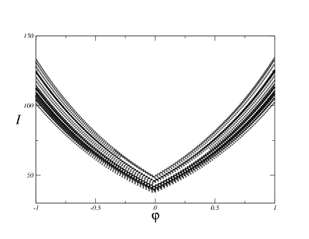
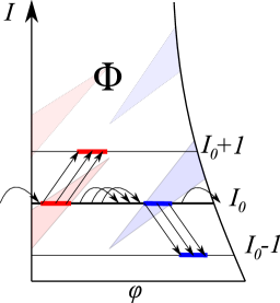
Figure 1. Left: typical trajectory in a phase space: $10^{6}$ iterations starting at $(\varphi_{0},\,I_{0})=(0.01,50)$. Right: First return map into fundamental domain $\Phi$. Schematic description of domains of positive, neutral and negative growth.

Our goal is to explain this behavior by renormalizing the induced transformation in the so-called fundamental domain $\Phi$. The fundamental domain is related to Poincaré section for flows in the sense that any orbit returns to it. In the Pinball map, we define the fundamental domain as the set of points $(\varphi,I)$ located between singular line $\varphi=0$ and its image

(5) $$\Phi=\{(\varphi,I)\in[0,2)\times[0,\infty],0<\varphi<{\rm Proj_{\varphi}}{\bf P}(0,I)\}.$$

The angular coordinate on $\Phi$ will be denoted by $\tilde{\varphi}\in[0,1]$.

Our first statement concerns the asymptotic description of the first return map:

Theorem 1.

Let $\mu=\exp(\alpha^{-1})$ and assume $0<\mu<3$. Let $\chi_{\mu}^{(0)}$ and $\chi_{\mu}^{(1)}$ be characteristic functions of the $\dfrac{1}{\mu}$ neighborhoods of the boundary of the fundamental domain, correspondingly, i.e. $\chi_{\mu}^{(0)}=\chi_{[0,\mu^{-1}]}$ and $\chi_{\mu}^{(1)}=\chi_{[1-\mu^{-1},1]}$.

Then, the first return map of the domain $\Phi$ under the map (4) is a $O(I^{-1})$ perturbation of the transformation

$$\begin{cases}\tilde{\varphi}_{1}=\tilde{\varphi}+\dfrac{2}{\mu}\,g_{\mu}(I,\tilde{\varphi})\mod 1\\ I_{1}=I+\chi_{+}(\tilde{\varphi}_{1})-\chi_{-}(\tilde{\varphi}_{1})\end{cases}$$

where $[\cdot]$ denotes an integer part and

$$g_{\mu}(I,\varphi)=\mathscr{H}_{\mu}(I-1-\chi_{\mu}^{(1)}(\varphi))+\frac{1}{2}(1+\chi_{+}+\chi_{-})-(\chi_{\mu}^{(0)}+\chi_{\mu}^{(1)})$$

where

$$\mathscr{H}_{\mu}(x)=\chi_{\geqslant 0}(\mu+2\{\mu x\}-3)-\{\mu x\}.$$

Functions $\chi_{+}$ and $\chi_{-}$ are characteristic functions of two intervals $\mathcal{I}_{+}$ and $\mathcal{I}_{-}$ respectively.

If $\mu$ is rational, then the map might possesses a uniformly growing trajectory. Indeed, if one of the periodic points stays longer in the positive part of the base interval than in the negative part, then the corresponding trajectory grows without bound. Our construction of an escaping trajectory of the system (4) consists in choosing the initial data in an appropriate way so as to kill the leading order perturbation of the map. Next, we would have to estimate that the remaining perturbation will not destroy such “resonant” growth. Combining these ideas, we prove

Theorem 2.

For $\alpha=\dfrac{1}{\ln 2m}$, $m\in\mathbb{N}$ there exists an unbounded trajectory in the system (4).

Remark 1.

If $\mu$ is irrational, then the leading order part of the map is reminiscent of EK map. Indeed, ignoring characteristic functions, the major part of the map takes the form

$$\tilde{\varphi}_{1}=\tilde{\varphi}+\frac{2}{\mu}-\{\mu(I-1)\}\,\,{\rm or}\,\,\tilde{\varphi}_{1}=\tilde{\varphi}+\frac{2}{\mu}-\{\mu(I-2)\}.$$

It seems likely that the angular variable will be uniformly distributed and one should expect similar behavior as found by Kesten. This will be the subject of future investigation.

Remark 2.

Note that smoothing the signum function discontinuity in (4) will make KAM theory applicable and then all solutions will be bounded.

Indeed, change the variables: $(\varphi,y)=(\varphi,I^{-1})$. In the new variables, the smooth version of the Pinball transformation takes the form

$$\begin{cases}\varphi_{1}=\varphi+\alpha y\mod 2\\ y_{1}=\dfrac{1}{\frac{1}{y}-f(\varphi,y)}\end{cases}$$

where $f$ is smooth and $|f(\varphi,y)|<1$. Then

$$y_{1}=y\dfrac{1}{1-yf(\varphi,y)}=y\left(1+\sum_{n=1}^{\infty}(yf(\varphi,y))^{n}\right)$$

so the perturbation is of order $O(y^{2})$ which is much smaller than the twist. The curve intersection property follows from the area-conservation in the original variables. Therefore, this map satisfies the conditions of monotone twist theorem, see e.g. [12].

4. Proof of Theorem 1.

Recall the definition of the fundamental domain as a subset $\Phi\subset\mathbb{S}\times\mathbb{R}_{+}$ between the discontinuity line $\phi=0$ and its first iteration:

(6) $$\Phi=\left\{(\varphi,I)\mid\varphi\in\left(0,\dfrac{\alpha}{I-1}\right)\right\}$$

and consider the transformation $T(\varphi,I)=(\varphi^{\prime},I^{\prime})$ as the first return map for any point $(\varphi,I)\in\Phi$ according to (4). We have the following bound on the action change

Lemma 1.

If $(\varphi^{\prime},I^{\prime})$ is an image of the point $(\varphi,I)$ under the transformation $T$ then $|I^{\prime}-I|\leqslant 1$.

In other words, Lemma 1 states that as the angle variable winds around the cylinder and the action variable undergoes large changes, after returning to the fundamental domain, the action will not change by more than 1. This property assures a good local control on the orbits.

Figure 2. Mapping from fundamental domain to itself represented on the base circle (left panel) and on the covering space (right panel).

Next, we describe the structure of the subsets in the base $\varphi\in(0,\alpha/(I-1))$ for which the action increases $I^{\prime}=I+1$ or decreases $I^{\prime}=I-1$.

Let us introduce the rescaled angle variable $\tilde{\varphi}=(I-1)\varphi\alpha^{-1}$. In the renormalized variables, the fundamental domain can be represented by

$$\Phi=(\tilde{\varphi},I)=[0,1]\times\mathbb{R}_{+}.$$

Lemma 2.

The set $\Phi\cap\{I=C\}$ is the union of three disjoint subsets

$$\Phi\cap\{I=C\}=\mathcal{I}_{+}\cup\mathcal{I}_{-}\cup\mathcal{I}_{0},$$

where $\mathcal{I}_{+}$ and $\mathcal{I}_{-}$ are intervals of equal measure and consist of all points $(\varphi,C)$ such that $T(\varphi,C)=(\cdot,C\pm 1)$ respectively.

The intervals are contained in the regions

$$\mathcal{I}_{+}\in\left(0,\frac{\alpha}{\mu(I-1)}\right)\,\,\,{\rm and}\,\,\,\mathcal{I}_{-}\in\left(\frac{\alpha(1-\mu^{-1})}{I-1},\frac{\alpha}{I-1}\right),$$

where $\mu(\alpha)=\exp(\alpha^{-1})$.

Finally, we have the following lemma which ends the proof of Theorem 1.

Lemma 3.

The first return map $T$ in the rescaled variables takes the form

$$T(\varphi,I)=\begin{cases}\tilde{\varphi}_{1}=\tilde{\varphi}+\dfrac{2}{\mu}\,\,g_{\mu}(I,\tilde{\varphi})+O(I^{-1})\\ I_{1}=I+\chi_{+}(\tilde{\varphi}_{1})-\chi_{-}(\tilde{\varphi}_{1})\end{cases}$$

where $\mu(\alpha)=\exp(\alpha^{-1})$, $\chi_{\pm}$ are characteristic functions of positive and negative intervals depending weakly on $I$.

5. Proofs

Proof of Lemma 1

Proof.

We begin with giving a heuristic argument based on the Figure 2 (right panel). We can represent orbits as stairs going up and down in the domain $\varphi\in[0,2]$. Consider the special configuration that is symmetric with respect to $\varphi=1$. It is easy to see that the corresponding solution will have the same action after the first return map. By moving the graph so that the top level does not cross $\varphi=1$ it is possible to see that the change in the action cannot be more than one. Indeed, the lowest level steps are wider than the top one and therefore at most one crossing can occur.

Now, we provide the full proof. Assume the initial point $(\varphi,I)$ is in the fundamental domain $\Phi$, i.e. $\varphi\in(0,\alpha/(I-1))$. The map (4) is iterated $n+1$ times while $I$ increases until the orbit is one step away from crossing $\varphi=1$. Next, the map is iterated $n^{\prime}+1$ times while $I$ decreases until the orbit is one step away from crossing $\varphi=2$. Then, by the definition of the fundamental domain, last $(n+n^{\prime}+2)$-nd iterate is in $\Phi$ and we obtain

(7) $$T(\varphi,I)=\left(\varphi+\alpha S_{1}(\varphi,I)+\alpha S_{2}(\varphi,I)+\dfrac{\alpha}{I+n+1}+\dfrac{\alpha}{I+(n-n^{\prime}-1)},I+n-n^{\prime}\right),$$

where

(8) $$S_{1}(\varphi,I)=\sum\limits_{k=0}^{n}\dfrac{1}{I+k},\qquad S_{2}(\varphi,I)=\sum\limits_{k=0}^{n^{\prime}}\dfrac{1}{I+n-k}.$$

The numbers $n$ and $n^{\prime}$ are uniquely defined by the relations:

(9) $$\begin{cases}1>\varphi+\alpha S_{1}(\varphi,I)\\ 1<\varphi+\alpha S_{1}(\varphi,I)+\dfrac{\alpha}{I+n+1}\end{cases}$$

and

(10) $$\left\{\begin{array}[]{cl}2>&\varphi+\alpha S_{1}(\varphi,I)+\alpha S_{2}(\varphi,I)+\dfrac{\alpha}{I+n+1}\\ \\ 2<&\varphi+\alpha S_{1}(\varphi,I)+\alpha S_{2}(\varphi,I)+\dfrac{\alpha}{I+n+1}+\dfrac{\alpha}{I+n-n^{\prime}-1}.\end{array}\right.$$

The equation (9) means that $n$-th iterate is the last one staying in the right half-circle, so the next iterate will be in the left half-circle. Similarly $(n+1)+n^{\prime}$-th iterate is the last one before returning to $\Phi$, see Figure 2.

Denote by $\Delta S=S_{2}-S_{1}$. Rewriting the second sum in (8) for $k^{\prime}=n-k$ we obtain for $\Delta S$:

(11) $$\Delta S=\sum\limits_{k^{\prime}=n-n^{\prime}}^{n}\dfrac{1}{I+k^{\prime}}-\sum\limits_{k=0}^{n}\dfrac{1}{I+k}.$$

Note that the expression (11) implies that

(12) $$\begin{cases}\Delta S>\dfrac{1}{I-1}+\dfrac{1}{I-2}&\mbox{ if }n-n^{\prime}<-1\\ \Delta S<-\dfrac{1}{I}-\dfrac{1}{I+1}&\mbox{ if }n-n^{\prime}>1.\end{cases}$$

To prove that $|n-n^{\prime}|\leqslant 1$ it is sufficient to show that (12) contradicts (9) – (10). Rewriting (10) for $S_{2}=\Delta S+S_{1}$ we obtain

(13) $$2>\varphi+2\alpha S_{1}(\varphi,I)+\alpha\Delta S+\frac{\alpha}{I+n+1}>2-\frac{\alpha}{I+n-n^{\prime}-1}.$$

Multiplying the equation (9) by $2$ and substituting into (13) we get

(14) $$\left\{\begin{array}[]{cl}\Delta S&<\dfrac{\varphi}{\alpha}+\dfrac{1}{I+n+1}\\ \\ \Delta S&>\dfrac{\varphi}{\alpha}-\dfrac{1}{I+n+1}-\dfrac{1}{I+n-n^{\prime}-1}.\end{array}\right.$$

Since for any point $(\varphi,I)\in\Phi$ one has $\dfrac{\varphi}{\alpha}\in\left(0,\dfrac{1}{I-1}\right)$ inequalities (14) contradict (12).

∎

Proof of lemma 2

Proof.

As already found in the proof of Lemma 1, transformation $T:\Phi\rightarrow\Phi$ in $\varphi$-variable takes the form

(15) $$\varphi^{\prime}=\varphi+\left(2\alpha S_{1}(\varphi,I)+\dfrac{\alpha}{I+n+1}-2\right)+\alpha\Delta S,$$

where

(16) $$\Delta S=\begin{cases}0,&{\rm if}\,\,\varphi\in\mathcal{I}_{+}\\ \dfrac{1}{I-1},&{\rm if}\,\,\varphi\in\mathcal{I}_{0}\\ \dfrac{1}{I-1}+\dfrac{1}{I-2},&{\rm if}\,\,\varphi\in\mathcal{I}_{-}\\ \end{cases}$$

Define $\delta_{1},\delta_{2}$ by the relations (see Fig. 2)

$$\varphi+\alpha S_{1}(\varphi,I)=1-\delta_{1}$$

$$\varphi+\alpha S_{1}(\varphi,I)+\dfrac{\alpha}{I+n+1}=1+\delta_{2},$$

then it is easy to see that

$$\varphi+2\alpha S_{1}(\varphi,I)+\dfrac{\alpha}{I+n+1}-2=\delta_{2}-\delta_{1}-\varphi.$$

Then the expression (16) could be rewritten in the form

(17) $$\begin{cases}\delta_{2}-\delta_{1}-\varphi>0,&\mbox{for}\quad\varphi\in\mathcal{I}_{+}\\ \delta_{2}-\delta_{1}-\varphi\in\left(-\dfrac{\alpha}{I-1},0\right),&\mbox{for}\quad\varphi\in\mathcal{I}_{0}\\ \delta_{2}-\delta_{1}-\varphi<-\dfrac{\alpha}{I-1},&\mbox{for}\quad\varphi\in\mathcal{I}_{-}\\ \end{cases}$$

In particular, the first inequality in (17) implies that for $\varphi\in\mathcal{I}_{+}$ one has

$$\varphi<\dfrac{\alpha}{I+n+1},\,\,{\rm since}\,\,\,\,\dfrac{\alpha}{I+n+1}=\delta_{2}+\delta_{1}.$$

Similarly, it is easy to verify that if $\varphi\in\mathcal{I}_{-}$ then $\varphi>\dfrac{\alpha}{I-1}-\dfrac{\alpha}{I+n+1}$. The next proposition describes some rigidity properties of the intervals $\mathcal{I}_{0},\mathcal{I}_{+},\mathcal{I}_{-}$ in (17)

Proposition 1.

Assume that $(\varphi_{0},I)\in\mathcal{I}_{+}$ and that the corresponding sum $S_{1}(\varphi_{0},I)$ has $n$ terms. Then the point $(\varphi_{\epsilon}=\varphi_{0}+\epsilon,I)$ belongs to $\mathcal{I}_{+}$ if and only if the sum $S_{1}(\varphi_{\epsilon},I)$ has also $n$ terms.

Proof.

Denote by $\delta_{1}^{(0)}$ and $\delta_{2}^{(0)}$ the corresponding parts of the interval $\dfrac{\alpha}{I+n+1}$ for the point $\varphi_{0}$. By assumption $\varphi_{0}\in\mathcal{I}_{+}$ and thus $\delta_{2}^{(0)}-\delta_{1}^{(0)}-\varphi_{0}>0$, then by (17) it is sufficient to verify that $\delta_{2}^{(\epsilon)}-\delta_{1}^{(\epsilon)}-\varphi_{\epsilon}$ remains positive.

Then the proof can be obtained from the following calculation:

(a) First, consider the case when the number of terms remains the same (equal to $n$). Then $\delta_{2}^{(\epsilon)}=\delta_{2}+\epsilon$, $\delta_{1}^{(\epsilon)}=\delta_{1}-\epsilon$ and so

(18) $$\delta_{2}^{(\epsilon)}-\delta_{1}^{(\epsilon)}-\varphi=(\delta_{2}^{(0)}+\epsilon)-(\delta_{1}^{(0)}-\epsilon)-\epsilon=\delta_{2}^{(0)}-\delta_{1}^{(0)}+\epsilon>\delta_{2}^{(0)}-\delta_{1}^{(0)}$$

(b) Assume now that the number of terms in $S_{1}(\varphi_{\epsilon},I)$ is different from $n$. Assume it contains $n-1$ terms (all other cases can be treated similarly). Then we have, see Figure 3.

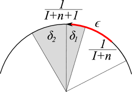
Figure 3. Rotation by $\epsilon$.

$$\delta_{2}^{(\epsilon)}=\epsilon-\delta_{1}^{(0)}=\epsilon+\delta_{2}^{(0)}-\dfrac{\alpha}{I+n+1}$$

which implies

$$\delta_{1}^{(\epsilon)}=\dfrac{\alpha}{I+n}-\delta_{2}^{(\epsilon)}=\dfrac{\alpha}{I+n}-\epsilon+\delta_{1}^{(0)}.$$

Finally, we have

$$\delta_{2}^{(\epsilon)}-\delta_{1}^{(\epsilon)}-\varphi_{\epsilon}=\epsilon+\delta_{2}^{(0)}-\delta_{1}^{(0)}-\varphi_{0}-\dfrac{\alpha}{I+n+1}-\dfrac{\alpha}{I+n}.$$

The latter expression is negative since by construction

$$\delta_{2}^{(0)}+\epsilon<\frac{1}{I+n}+\frac{1}{I+n+1}.$$

This ends the proof of the proposition. ∎

Using proposition 1, we will find the set $\mathcal{I}_{+}$. Let the initial angle be $\varphi_{0}=0$ then

$$\delta_{2}^{(0)}~{}=~{}\left\{\alpha\sum\limits_{j=0}^{n+1}\dfrac{1}{I+j}\right\}\,\,{\rm and}\,\,\delta_{1}^{(0)}=\dfrac{\alpha}{I+n+1}-\delta_{2}^{(0)}.$$

If $\delta_{2}^{(0)}>\delta^{(0)}_{1}$ then by (17) the point $(0,I)$ belongs to $\mathcal{I}_{+}$ and then proposition 1 implies that $\mathcal{I}_{+}=\left(0,\delta_{1}^{(0)}\right)$.

Otherwise, if $\delta_{2}^{(0)}<\delta^{(0)}_{1}$ then $(0,I)$ does not belong to $\mathcal{I}_{+}$ and to find the leftmost point $(\phi=\epsilon,I)\in\mathcal{I}_{+}$ we need to satisfy the condition $\delta_{2}^{(\epsilon)}-\delta_{1}^{(\epsilon)}-\epsilon>0$. Using (18) we obtain $\epsilon=\delta_{1}^{(0)}-\delta_{2}^{(0)}$ and therefore in this case $\mathcal{I}_{+}=\left(\delta_{1}^{(0)}-\delta_{2}^{(0)},\delta_{1}^{(0)}\right)$.

Similar calculations can be carried out for $\mathcal{I}_{-}$, but it is easier to use symmetric properties of the map with respect to reversing the “time”.

Then, if $\delta_{1}^{(00)}>\delta^{(00)}_{2}$ ($\delta_{i}^{(00)}$ correspond to $\delta^{(0)}$ but are obtained from negative iterates) the point $(0-,I-1)$ which is the preimage of $(\frac{\alpha}{I-1}-,I)$ belongs to $\mathcal{I}_{-}$ and by the same argument as above for $\mathcal{I}_{+}$, we have

$$\mathcal{I}_{-}=\left(\frac{\alpha}{I-1}-\delta_{2}^{(00)},\frac{\alpha}{I-1}\right).$$

If the converse holds, i.e. $\delta_{2}^{(00)}>\delta^{(00)}_{1}$ we obtain

$$\mathcal{I}_{-}=\left(\frac{\alpha}{I-1}-(\delta_{2}^{(00)}-\delta_{1}^{(00)}),\frac{\alpha}{I-1}-\delta_{2}^{(00)}\right).$$

This ends the proof of the lemma. ∎

The location and the measure of the intervals $\mathcal{I}_{+}$ and $\mathcal{I}_{-}$ are then controlled by the fractional parts of the sums $\alpha S_{1}(0,I)$. We shall estimate these quantities in the proof of the next lemma.

Proof of Lemma 3

Proof.

For the clarity of presentation, we give the proof only for the case $I=N$. The general case can be treated similarly. We introduce the notation for the expression

$$\alpha\psi(\varphi,I)=2\alpha S_{1}(\varphi,I)+\frac{\alpha}{I+n+1}-2$$

from (15).

In the rescaled variables, the transformation (15) takes the form

(19) $$\tilde{\varphi}^{\prime}=\begin{cases}\frac{I}{\alpha}\varphi^{\prime}=\left(1+\dfrac{1}{I-1}\right)\tilde{\varphi}+I\psi(I,\varphi),&\varphi\in\mathcal{I}_{+}\\ \frac{I-1}{\alpha}\varphi^{\prime}=\tilde{\varphi}+(I-1)\psi(I,\varphi)+1,&\varphi\in\mathcal{I}_{0}\\ \frac{I-2}{\alpha}\varphi^{\prime}=\left(1-\dfrac{1}{I-1}\right)\tilde{\varphi}+(I-2)\psi(I,\varphi)+2-\dfrac{1}{I-1},&\varphi\in\mathcal{I}_{-}\end{cases}$$

Case $\varphi\in\mathcal{I}_{+}$. If the action variable $I$ increases, then the number $n$ of iterates of the transformation (4) contained in the right half-circle (where the action is gained) is greater than the number $n^{\prime}$ of iterates contained in the left half-circle. Lemma 1 implies that $n=n^{\prime}+1$. Thus, the transformation $T$ for these values of $\varphi$ takes the form

$$\varphi^{\prime}=\varphi+2\alpha S_{1}(\varphi,I)+\dfrac{\alpha}{I+n+1}-2,$$

where

$$S_{1}(\varphi,N)=\sum\limits_{k=0}^{n}\dfrac{1}{N+k},$$

Proposition 2.

Assume that $\mu\in(1,3)$, then for $\varphi\in\mathcal{I}_{+}$ the number $n$ is given by

(20) $$n=\mu(N-1)-N+\mathscr{H}_{\mu}(N-1),$$

where $\mu=\exp(1/\alpha)$ and

$$\mathscr{H}_{\mu}(x)=\chi_{\geqslant 0}(\mu+2\{\mu x\}-3)-\{\mu x\}.$$

Remark 3.

If $\mu>3$, then an additional term $\left[\frac{\mu-1}{2}\right]$ has to be added in (20). We omit the detailed calculations of this more general case, which can be reproduced in the same way.

Proof.

By proposition 1, the number of steps in the positive half of the cylinder $n$ is independent of $\varphi\in\mathcal{I}_{+}$, therefore it is sufficient to verify (20) only for some $\varphi\in\mathcal{I}_{+}$ using (9). Moreover, we can take $\varphi=0$ even though this point might not be in $\mathcal{I}_{+}$. Indeed, according to lemma 2 the point $\varphi=0$ satisfies $\varphi\in\mathcal{I}_{+}$ or $\varphi\in\mathcal{I}_{0}$. If the former, we are done. If the latter then it is possible to see that by increasing $\varphi$ we will eventually cross into $\mathcal{I}_{+}$ without changing $n$ (the number of steps in positive part of the cylinder).

We have

$$S_{1}(\varphi,N)=\sum\limits_{k=0}^{n}\dfrac{1}{N+k}=H_{N+n}-H_{N-1},$$

where $H_{k}$ denotes $k$-th harmonic number. The harmonic number has the following asymptotic expansion

$$H_{k}=\ln k+\gamma+\dfrac{1}{2k}-\sum\limits_{j=1}^{\infty}\dfrac{B_{2j}}{2jk^{2j}}$$

where $B_{j}$ denotes $j$-th Bernoulli number. Therefore,

(21) $$\begin{split}S_{1}(\varphi,N)=\ln\dfrac{N+n}{N-1}&+\dfrac{1}{2}\left(\dfrac{1}{N+n}-\dfrac{1}{N-1}\right)-\dfrac{1}{12}\left(\dfrac{1}{(N+n)^{2}}-\dfrac{1}{(N-1)^{2}}\right)+O\left(\dfrac{1}{N^{4}}\right)\end{split}$$

We will take $n=[\mu(N-1)]-N+\gamma$ and will verify that $\gamma$ is given by the above Heaviside function.

Using the relation $[\mu(N-1)]=\mu(N-~{}1)-~{}\{\mu(N-~{}1)\}$ and denoting $\ell:=\dfrac{\gamma}{\mu(N-1)}$ and $y:=~{}\dfrac{\{\mu(N-1)\}}{\mu(N-1)}$ we can rewrite (20)

$$N+n=\mu(N-1)(1-y+l).$$

Substituting this expression into (21) we obtain

$$\begin{split}S_{1}(\varphi,N)=\ln\mu(1-(y-l))+\dfrac{1}{2(N-1)}\left(\dfrac{1}{\mu(1-(y-l))}-1\right)\\ -\dfrac{1}{12(N-1)^{2}}\left(\dfrac{1}{\mu^{2}(1-(y-l))^{2}}-1\right)+O\left(\dfrac{1}{N^{4}}\right).\end{split}$$

Now, we expand the expression for $S_{1}$ in the perturbation series using

$$\ln(\mu(1-(y-l)))=\ln\mu-\sum\limits_{j=1}^{\infty}\frac{(y-l)^{j}}{j},\qquad\frac{1}{\mu(1-(y-l))}=\frac{1}{\mu}\sum\limits_{j=0}^{\infty}(y-l)^{j},$$

and

$$\frac{1}{\mu^{2}(1-(y-l))^{2}}=\frac{1}{\mu^{2}}\sum\limits_{j=0}^{\infty}(j+1)(y-l)^{j}.$$

Collecting all the terms of the same order in $N$ up to $O(y)$ and $O(N^{-3})$

(22) $$\begin{split}S_{1}(\varphi,N)=\ln\mu&+\dfrac{1}{2(N-1)}\left(\frac{1+2\gamma-2\{\mu(N-1)\}}{\mu}-1\right)\\ &-\frac{1}{12(N-1)^{2}}\left(\dfrac{6\gamma(\gamma+1)}{\mu^{2}}-1\right)+O\left(y,N^{-3}\right).\end{split}$$

We need to choose $\gamma$ in such a way that $\alpha S_{1}<1$ but $\alpha S_{1}+\frac{1}{N+n+1}>1$.

Recalling that $\alpha=\dfrac{1}{\ln\mu}$ and that the leading contribution for deviation from 1, is controlled by terms of order $1/(N-1)$, we must assure

$$1+2\gamma-2\{\mu(N-1)\}<\mu,$$

but

$$1+2\gamma-2\{\mu(N-1)\}+2>\mu.$$

The additional summand 2 comes from

$$\dfrac{1}{N+n+1}=\dfrac{1}{[\mu(N-1)]+\gamma+1}=\dfrac{2}{2\mu(N-1)}+O(1/N^{2}).$$

We rewrite two inequalities in a more compact form

$$1<\mu+2\{\mu(N-1)\}-2\gamma<3.$$

Now, if $\gamma=0$, then clearly left side of the inequality holds, since $\mu>1$, and then right side would also hold provided $\mu+2\{\mu(N-1)\}<3$. Thus, $\gamma=0$ if $\mu+2\{\mu(N-1)\}<3$.

If, on the other hand, $\mu+2\{\mu(N-1)\}>3$, we can take $\gamma=1$ as the left side of the inequality will hold. The right side will also hold if apply the assumption $\mu<3$. Therefore, we can finally conclude $\gamma=\chi_{\geqslant 0}(\mu+2\{\mu(N-1)\}-3).$

∎

Now, we will derive an explicit expression for the first return map $T$. Multiply (22) by $2\alpha$

(23) $$\begin{split}2\alpha S_{1}(\varphi,N)&=2+\dfrac{\alpha}{N-1}\left(\dfrac{1+2\mathscr{H}_{\mu}(N-1)}{\mu}-1\right)-\\ &-\dfrac{\alpha}{6(N-1)^{2}}\left(\dfrac{6(\,\chi_{\geqslant 0}(N-1)+1)\,\chi_{\geqslant 0}(N-1)}{\mu^{2}}-1\right)+O\left(y,N^{-3}\right).\end{split}$$

So we get for $\psi(\varphi,N)$

$$\begin{split}&\alpha\psi(\varphi,N)=2\alpha S_{1}(\varphi,N)+\dfrac{\alpha}{\mu(N-1)+\mathscr{H}_{\mu}(N-1)+1}-2=\\ &=\dfrac{\alpha}{N-1}\left(\dfrac{1+2\mathscr{H}_{\mu}(N-1)}{\mu}-1\right)-\dfrac{\alpha}{6(N-1)^{2}}\left(\dfrac{6(\,\chi_{\geqslant 0}(N-1)+1)\,\chi_{\geqslant 0}(N-1)}{\mu^{2}}-1\right)+\\ &+\dfrac{\alpha}{\mu(N-1)}\left(1-\dfrac{\mathscr{H}_{\mu}(N-1)+1}{\mu(N-1)}\right)+O\left(y,N^{-3}\right).\end{split}$$

And finally (using that $\chi_{\geqslant 0}^{2}=\chi_{\geqslant 0}$), we have

(24) $$\begin{split}\varphi^{\prime}=\varphi+\alpha\psi(\varphi,I)=&\varphi+\frac{\alpha}{N-1}\left(\dfrac{2+2\mathscr{H}_{\mu}(N-1)}{\mu}-1\right)-\\ -&\dfrac{\alpha}{(N-1)^{2}}\left(\dfrac{\mathscr{H}_{\mu}(N-1)+2\,\chi_{\geqslant 0}(N-1)+1}{\mu^{2}}+\dfrac{1}{6}\right)+O\left(y,N^{-3}\right).\end{split}$$

Multiplying both sides of the equation (24) by the scaling factor $\dfrac{N-1}{\alpha}$ we obtain

(25) $$\begin{split}\dfrac{N-1}{\alpha}\varphi^{\prime}=\tilde{\varphi}+&\left(\dfrac{2+2\mathscr{H}_{\mu}(N-1)}{\mu}-1\right)-\\ -&\dfrac{\alpha}{N-1}\left(\dfrac{\mathscr{H}_{\mu}(N-1)+2\,\chi_{\geqslant 0}(N-1)+1}{\mu^{2}}-\dfrac{1}{6}\right)+O\left(y,N^{-2}\right).\end{split}$$

Since $\varphi\in\mathcal{I}_{+}$ we can use (19)

$$\tilde{\varphi}^{\prime}=\dfrac{N}{\alpha}\varphi^{\prime}=\left(1+\dfrac{1}{N-1}\right)\dfrac{N-1}{\alpha}\varphi^{\prime}.$$

Thus, in the leading order in the rescaled variables, the transformation takes the form

$$\tilde{\varphi}^{\prime}=\tilde{\varphi}+\dfrac{2}{\mu}(1+\mathscr{H}_{\mu}(N-1))-1$$

Case $\varphi\in\mathcal{I}_{-}$. By the direct calculations, one obtains

$$\tilde{\varphi}^{\prime}=\tilde{\varphi}+\dfrac{2}{\mu}(1+\mathscr{H}_{\mu}(N-2))-1.$$

Indeed, moving in the opposite direction, we have

$$\frac{\alpha}{N-1}-\varphi=\frac{\alpha}{N-2}-\varphi^{\prime}+\frac{\alpha}{N-2}\left(\dfrac{2+2\mathscr{H}_{\mu}(N-2)}{\mu}-1\right).$$

Neglecting terms of order $O(N^{-2})$ and rearranging the terms , we obtain

$$\varphi^{\prime}=\varphi+\frac{\alpha}{N-2}\left(\dfrac{2+2\mathscr{H}_{\mu}(N-2)}{\mu}-1\right).$$

Multiplying with $(N-2)/\alpha$,

$$\tilde{\varphi}^{\prime}=\tilde{\varphi}\,\frac{N-2}{N-1}+\left(\dfrac{2+2\mathscr{H}_{\mu}(N-2)}{\mu}-1\right)$$

we arrive at the above formula since there we neglect terms of order $O(N^{-1})$.

Case $\varphi\in\mathcal{I}_{0}$. We already know that $\mathcal{I}_{0}$ is either a single interval with $\mathcal{I}_{+}$ and $\mathcal{I}_{-}$ complementing it to the full fundamental interval or $\mathcal{I}_{0}$ consists of three intervals. In the latter case, $\mathcal{I}_{+}$ and $\mathcal{I}_{-}$ are located in the interior of the fundamental domain, while three intervals of $\mathcal{I}_{0}$ complement at the left boundary, right boundary and in the middle between $\mathcal{I}_{+}$ and $\mathcal{I}_{-}$.

First, consider the case of the middle interval of $\mathcal{I}_{0}$ which can be the whole set $\mathcal{I}_{0}$ or part of it, as explained above. Compared to the $\mathcal{I}_{+}$ case, $n$, the number of steps in the positive side of the cylinder decreases by 1, i.e.

$$n=\mu(N-1)-N+\mathscr{H}_{\mu}(N-1)-1.$$

Next, we follow the previous calculation of the transformation $T$ on $\mathcal{I}_{+}$ indicating the changes. First, recall that on $\mathcal{I}_{0}$, we always have

$$\varphi^{\prime}=\varphi+2\alpha S_{1}(\varphi,I)-2.$$

Thus, we can modify (23) for our case by subtracting 1 from $\mathscr{H}$

$$2\alpha S_{1}=2+\frac{\alpha}{N-1}\left(\frac{1+2(\mathscr{H}_{\mu}(N-1)-1)}{\mu}-1\right).$$

Next using $\alpha\psi=2\alpha S_{1}-2$, we have

$$\varphi^{\prime}=\varphi+\frac{\alpha}{N-1}\left(\frac{1+2(\mathscr{H}_{\mu}(N-1)-1)}{\mu}-1\right)$$

and renormalizing

$$\tilde{\varphi}^{\prime}=\tilde{\varphi}+\frac{1+2(\mathscr{H}_{\mu}(N-1)-1)}{\mu}-1.$$

After slight simplifications, we finally have

$$\tilde{\varphi}^{\prime}=\tilde{\varphi}+\frac{2}{\mu}(\mathscr{H}_{\mu}(N-1)-1/2)-1.$$

Now, we consider the leftmost subinterval of $\mathcal{I}_{0}$, if it exists. By previous arguments, $n$ is the same as for the $\mathcal{I}_{+}$, so we have

$$2\alpha S_{1}=2+\frac{\alpha}{N-1}\left(\frac{1+2\mathscr{H}_{\mu}(N-1)}{\mu}-1\right).$$

Using again $\alpha\psi=2\alpha S_{1}-2$ and following the same calculations, we find

$$\tilde{\varphi}^{\prime}=\tilde{\varphi}+\frac{2}{\mu}(\mathscr{H}_{\mu}(N-1)+1/2)-1,$$

The last case is the rightmost subinterval of $\mathcal{I}_{0}$ if it exists. Similar argument leads to

$$\tilde{\varphi}^{\prime}=\tilde{\varphi}+\frac{2}{\mu}(\mathscr{H}_{\mu}(N-2)+1/2)-1.$$

∎

5.1. Proof of Theorem 2

Proof.

If $\alpha=\dfrac{1}{\ln n}$ then $\mu=n$ and therefore $y\equiv 0$. Thus, all the terms in series expansion (25) depending on $y$ vanish and we get only $O(N^{-3})$ terms. In the leading order, the rescaled transformation takes the form

$$\tilde{\varphi}^{\prime}=\tilde{\varphi}+\left(\dfrac{2\left(1+\left[\frac{\mu-1}{2}\right]\right)}{\mu}-1\right),$$

for $\tilde{\varphi}\in\mathcal{I}_{+}$.

For our particular choice $\mu=2m$ we have $\left[\frac{\mu-1}{2}\right]=m-1$ and so in the leading order the transformation $T$ is the identity map. To simplify an analysis consider only the case $\mu=\ln 2$. Other cases can be treated similarly. Thus, we get

$$\tilde{\varphi}^{\prime}=\tilde{\varphi}+\frac{1}{8(N-1)}-\frac{1}{4N-2}+O(N^{-2})$$

To construct an unbounded orbit, we search for an initial point $\tilde{\varphi}_{0}$ satisfying two conditions:

• $\chi_{+}(\tilde{\varphi}_{0})=1$,

• The image $\tilde{\varphi}^{\prime}_{0}$ under the transformation $T$ coincides with initial angle up to the new normalization $\tilde{\tilde{\varphi}}_{0}$.

Note that for a larger action variable the scaling factor would be different. Therefore, we have

$$\tilde{\tilde{\varphi}}_{0}=\dfrac{N-1}{N}\tilde{\varphi}_{0}=\tilde{\varphi}_{0}-\frac{1}{N}\tilde{\varphi}_{0}$$

and the “renormalized fixed point” condition yields

$$\tilde{\varphi}_{0}-\frac{1}{N}\tilde{\varphi}_{0}=\tilde{\varphi}_{0}+\frac{1}{8(N-1)}-\frac{1}{4N-2}+O(N^{-3}).$$

Thus, up to the order $O(N^{-3})$

$$-\frac{\tilde{\varphi}_{0}}{N}=\frac{4N-2-8N+8}{8(N-1)(4N-2)}=-\frac{2N-3}{8(N-1)(2N-1)}=$$

$$=-\frac{1}{8(N-1)}+\frac{1}{4(N-1)(2N-1)}=-\frac{1}{8N}-\frac{1}{8N(N-1)}+\frac{1}{4(N-1)(2N-1)}=$$

$$=-\frac{1}{8N}+\frac{1}{4(N-1)}\left(\frac{1}{2N}-\frac{1}{2N-1}\right)=-\frac{1}{8N}-\frac{1}{8N(N-1)(2N-1)}.$$

As a result, for $\tilde{\varphi}_{0}=\dfrac{1}{8}+O(N^{-3})$ its image under first return map is given by $\tilde{\varphi}^{\prime}_{0}=\dfrac{1}{8}+O(N^{-3})$.

To check the first statement $\chi_{+}(\varphi_{0})=1$ it is sufficient to show that $\varphi_{0}+2\alpha S_{1}+\dfrac{\alpha}{N+n+1}$ is greater than $2$. This immediately follows from (23) and the estimate

$$\varphi_{0}+2\alpha S_{1}+\dfrac{\alpha}{N+n+1}>\dfrac{1}{8N\ln 2}+2-\dfrac{1}{\ln 2(2N-2)}+O(N^{-2})+\dfrac{1}{(2N-1)\ln 2}>2.$$

∎

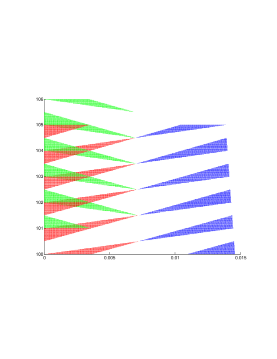
Figure 4. The structure of the fundamental domain for $\alpha=\dfrac{1}{\log 2}$. The regions of positive growth are in red and their images are in green. The regions of negative growth are in blue.

Remark 4.

For $\mu=2m+1$, $m\in\mathbb{N}$ rotation number for the map equals $(\mu-1)/\mu$ which guarantees that any trajectory could not hit $\mathcal{I}_{+}$ two successive times. Moreover such map has a fixed point in the set $\mathcal{I}_{0}$. However since renormalization for the neutral set is an identity map, drift produced by the second order term could not be compensated. We conjecture that in this case one could possibly derive an exponential bounds on the rate of action growth for the map $T$.

Remark 5.

We conjecture also that the same arguments as in Lemmas 1 – 3 can be used for other values of $\mathsf{z}\in(-1,0)$. Here instead of asymptotic expansion for harmonic numbers one should use generalized harmonic numbers $H_{n,\mathsf{z}}$. Since $H_{n,\mathsf{z}}\to\zeta(k)$ as $n\to\infty$ one can establish the relation for $H_{(I+n),\mathsf{z}}-H_{(I-1),\mathsf{z}}=2$ to find the expression for $n$. Arguments in Lemma 1, 2 and 3 can be applied with minor changes.

Appendix A

In the appendix we give more detailed derivation of some specific problems that lead to $\alpha\mathsf{z}$ map.

Example 1: Particle in switching potential

Consider a classical particle moving on the line in the square wave potential $V(x)=(-1)^{[x]}$ and assume the potential is switched every time unit $V(x,t)=(-1)^{[t]}\cdot(-1)^{[x]}$. While such potential is not differentiable, there is a natural way to define the dynamics by using the energy relation: the kinetic energy changes by 2 if the particle passes $t\in{\mathbb{Z}}$ integer points. We should ignore the singular subset of the extended phase space $(t,\dot{x},x)$ where there is discontinuity in both time and space and the dynamics is not defined. Such subset has zero measure. Outside the singular set particle moves with constant speed $v(x,t)=\sqrt{E-V(x,t)}$.

Since the dynamics defined for $x\mod{2}$, $t\mod{2}$ we can project the dynamics on a plane onto the system on a cylinder $[0,2)\times\mathbb{R}_{+}$. Write the Hamiltonian form of the unit time step transformation for this system. Hamiltonian has a form $H(x,\dot{x},t)=\frac{\dot{x}^{2}}{2}+V^{\prime}(x,t)$ and so for the canonical action-angle variables we get

(26) $$\begin{cases}I_{\pm}=\sqrt{2(H-1)}+\sqrt{2(H+1)}\\ \varphi_{\pm}=\dfrac{1}{T}\left(\dfrac{x-1}{\sqrt{2(H\pm\mathrm{sgn}(x-1))}}+\dfrac{1}{\sqrt{2(H\mp 1)}}\right)\end{cases}$$

Here $T=\left(\dfrac{1}{\sqrt{2(H-1)}}+\dfrac{1}{\sqrt{2(H+1)}}\right)$ is a period of rotation along the level curve $H(x,\dot{x})=H$ and $(\varphi_{\pm},I_{\pm})$ correspond to the angle-action variables for odd/even values of $[t]$. To deduce the system in action-angle variables, write down a generating function. For Hamiltonian we have

$$H(x,\dot{x},t)=H_{0}(I,t)+\partial_{3}S_{\pm}(x(t),I,t)$$

Where

$$\begin{cases}S_{+}(x,I)=(x-1)\sqrt{2(I+\mathrm{sgn}(x-1))}+\sqrt{2(I-1)}\\ S_{-}(I)=iS_{+}(-I)\end{cases}$$

Or, using (26)

$$S_{+}=\begin{cases}2T(I+1)\varphi_{+}-\dfrac{4}{\sqrt{2(I-1)}},\,x>1\\ 2T(I-1)\varphi_{+},\,x<1\end{cases}$$

Finally, the total system in variables $(\varphi,I)$ can be deduced from the expression (26) and the relation $\varphi_{\pm}=\partial_{I}S_{\pm}$.

(27) $$\begin{cases}\varphi_{1}=(\varphi+\alpha\sqrt{I})\mod{2}\\ I_{1}=I+\mathrm{sgn}(\varphi_{1}-1)\end{cases}$$

where $\alpha$ is some constant. Clearly, this system can be considered as a particular example of transformation (2) with $\mathsf{z}=\frac{1}{2}$.

Example 2: Fermi-Ulam acceleration.

In Fermi-Ulam problem the particle bounces between two walls. Assume that one wall is at rest $x=0$ and the other moves periodically $x=p(t)$, $p(t+1)=p(t)>0$. There is a standard transformation “stopping” the wall, see e.g. [16] with

$$x=p(t)y,\,\,\,\tau=\int_{0}^{t}\frac{ds}{p^{2}(s)}ds.$$

In the new variables, the equation takes the form

$$y^{\prime\prime}+\ddot{p}p^{3}y=0,$$

where $\prime$ denotes the derivative with respect to $\tau$. Evaluating the one period map, under the assumption that $p$ is piecewise linear, we obtain

(28) $$\begin{cases}y_{2}=(y_{1}+y_{1}^{\prime})\mod{1}\\ y_{2}^{\prime}=y_{1}^{\prime}+y_{2}\,\mathrm{sgn}\,(y_{2}-1/2).\end{cases}$$

This mapping is not a particular case of $\alpha\mathsf{z}$-map but it corresponds to the linear growth of the action when $\mathsf{z}=1$. While showing unbounded growth is relatively easy in this case, more challenging problem is to estimate the relative measure of bounded solutions. This has been done in [2].

Example 3: Outer billiards with degenerate boundary.

Consider the outer billiard system. Let $\gamma$ be a smooth strictly convex curve on the plane. Take any point $x\in\mathbb{R}^{2}$ outside of $\gamma$ and let $l(x)$ be a ray tangent to $\gamma$ and oriented in the counter-clockwise direction. There is another point on the ray $T(x)$ which has the same distance to the tangency point as $x$. This defines the outer billiard map, see e.g. [15]. A natural question is whether all the orbits are bounded. Thus, one is led to study this map for large $x$.

Assume that $\gamma$ is a unit circle centered at the origin, then for large $x$ the square of the map $T^{2}$ is close to identity and it leaves concentric circles invariant. The angle changes by a factor of $1/|x|$, which corresponds to $\mathsf{z}=-1$ in the $\alpha\mathsf{z}$-map. Now, consider the circle with a small circle segment removed. Then, the map becomes a small discontinuous perturbation of the above integrable map. When, $\gamma$ is half the circle, the outer billiard has unbounded orbit, see [4, 3].

Earlier, Schwartz [14] constructed unbounded orbits for quadrilateral $\gamma$ .

Aknowlegments.

First author (M.A.) was supported by AFOSR MURI grant FA9550-10-1-0567. The research of V.Z. was partially supported by NSF DMS-0807897.

References

- [1] M. Arnold, G. Dobrushina, E. Dinaburg, S. Pirogov, and A. Rybko. On products of skew rotations. Moscow Math. J., 2012.
- [2] J. de Simoi and D. Dolgopyat. Dynamics of some piecewise smooth fermi-ulam models. Chaos: An Interdisciplinary Journal of Nonlinear Science, 22(2):026124, 2012.
- [3] D. Dolgopyat and B. Fayad. Unbounded orbits for semicircular outer billiard. Ann. Henri Poincaré, 10(2):357–375, 2009.
- [4] D. Genin. Hyperbolic outer billiards: a first example. Nonlinearity, 19(6):1403–1413, 2006.
- [5] M.-R. Herman. Sur les courbes invariantes par les difféomorphismes de l’anneau. Vol. 1, volume 103 of Astérisque. Société Mathématique de France, Paris, 1983. With an appendix by Albert Fathi, With an English summary.
- [6] V. Kaloshin. Geometric proofs of Mather’s connecting and accelerating theorems. In Topics in dynamics and ergodic theory, volume 310 of London Math. Soc. Lecture Note Ser., pages 81–106. Cambridge Univ. Press, Cambridge, 2003.
- [7] V. Kaloshin and M. Levi. Geometry of Arnold diffusion. SIAM Rev., 50(4):702–720, 2008.
- [8] H. Kesten. On a conjecture of Erdös and Szüsz related to uniform distribution mod 1. Acta Arith., 1966.
- [9] S. Laederich and M. Levi. Invariant curves and time-dependent potentials. Ergodic Theory and Dynamical Systems, 11:365–378, 5 1991.
- [10] Mark Levi. Quasiperiodic motions in superquadratic time-periodic potentials. Comm. Math. Phys., 143(1):43–83, 1991.
- [11] D. Liberzon. Switching in Systems and Control. Systems & Control. Birkhäuser, 2003.
- [12] J. Mather and G. Forni. Action minimizing orbits in Hamiltonian systems. In Transition to chaos in classical and quantum mechanics (Montecatini Terme, 1991), volume 1589 of Lecture Notes in Math., pages 92–186. Springer, Berlin, 1994.
- [13] D. Ralston. Substitutions and 1/2-discrepancy of . Acta Arith., 2012.
- [14] R.E. Schwartz. Outer Billiards on Kites. Princeton University Press, 2009.
- [15] S. Tabachnikov. Billiards. Panor. Synth., (1):vi+142, 1995.
- [16] V. Zharnitsky. Instability in Fermi-Ulam “ping-pong” problem. Nonlinearity, 11(6):1481–1487, 1998.