WASP-8b: Characterization of a Cool and Eccentric Exoplanet with Spitzer

Abstract

WASP-8b has 2.18 times Jupiter’s mass and is on an eccentric ($e=0.31$) 8.16-day orbit. With a time-averaged equilibrium temperature of 948 K, it is one of the least-irradiated hot Jupiters observed with the Spitzer Space Telescope. We have analyzed six photometric light curves of WASP-8b during secondary eclipse observed in the 3.6, 4.5, and 8.0 m Infrared Array Camera bands. The eclipse depths are $0.113\pm 0.018$%, $0.069\pm 0.007$%, and $0.093\pm 0.023$%, respectively, giving respective brightness temperatures of 1552, 1131, and 938 K. We characterized the atmospheric thermal profile and composition of the planet using a line-by-line radiative transfer code and a Markov-chain Monte Carlo sampler. The data indicated no thermal inversion, independently of any assumption about chemical composition. We noted an anomalously high 3.6-m brightness temperature (1552 K); by modeling the eccentricity-caused thermal variation, we found that this temperature is plausible for radiative time scales less than $\sim 10^{2}$ hours. However, as no model spectra fit all three data points well, the temperature discrepancy remains as an open question.

1. Introduction

When transiting exoplanets pass behind their host stars (a secondary eclipse), the observed flux drop provides a direct measurement of the planet’s thermal emission and reflected light. Today, secondary-eclipse observations exist for nearly 30 exoplanets. The Spitzer Space Telescope (Werner et al., 2004) made most of these observations, capturing broadband photometric light curves in six near- and mid-infrared bands (3–24 m). Each band probes a specific altitude range in a planet’s atmosphere. With Bayesian fitting of model spectra, one can quantitatively constrain the atmospheric chemical composition and thermal profile of the planet’s photosphere (Madhusudhan & Seager, 2010). WASP-8b, with a time-averaged equilibrium temperature of 948 $\pm$ 22 K ($T$eq, temperature at which blackbody emission balances absorbed energy, assuming zero albedo and efficient heat redistribution), is one of the coolest Jupiter-sized planets yet observed in eclipse, and thus serves as an end member to the set of measured hot-Jupiter atmospheres.

To classify the hot-Jupiter population, Fortney et al. (2008) proposed a separation between moderately and strongly irradiated planets. The higher atmospheric temperatures of the more strongly irradiated planets allow the presence of highly opaque molecules (like TiO and VO) at high altitudes. These strong absorbers produce hot stratospheres (thermal inversion layers). In contrast, for the moderately irradiated hot Jupiters, these absorbers condense and rain out to altitudes below the photosphere, thus presenting no thermal inversions.

In general, the observations agree with this hypothesis, but exceptions indicate that the picture is not yet completely understood. For example, secondary-eclipse observations of the highly irradiated WASP-12b (Madhusudhan et al., 2011; Crossfield et al., 2012), WASP-14b (Blecic et al., 2013), and TrES-3 (Fressin et al., 2010) do not show evidence of thermal inversions. Conversely, XO-1 has an inversion layer even though it receives a much lower stellar irradiation (Machalek et al., 2008). Photochemistry provides one explanation. The non-equilibrium atmospheric chemistry models of Zahnle et al. (2009) suggested that heating from sulfur compounds in the upper atmospheres of hot Jupiters could explain these inversions. Alternatively, Knutson et al. (2010) suggest that strong UV radiation from active stars destroys the high-altitude absorbers.

The Wide-Angle Search for Planets (WASP) Consortium discovered WASP-8b in 2008 (Queloz et al., 2010). The planet orbits the brighter component (WASP-8A) of a binary stellar system. The angular separation (4.83″) with the secondary (WASP-8B) sets a minimum separation of 440 AU between the stars. WASP-8A is a G6 star, with effective temperature $T$eff = 5600 K. Color and photometric analyses indicate that WASP-8B is a colder M star (Queloz et al., 2010). WASP-8b is a 2.18 Jupiter-mass ($M$Jup) planet with 1.08 times Jupiter’s radius ($R$Jup) in a retrograde 8.16 day orbit. Its large eccentricity ($e=0.31$) should make the planet’s dayside temperature vary by hundreds of degrees along the orbit, possibly forcing an unusual climate.

The age of the host star (4 Gyr) is shorter than the planet’s orbital circularization time ($\sim$30 Gyr, see, e.g., Goldreich & Soter, 1966; Bodenheimer et al., 2001); accordingly, WASP-8b has one of the most eccentric orbits among the $\sim$10-day-period exoplanets (Pont et al., 2011). The Kozai mechanism (Wu & Murray, 2003) may explain the combination of high eccentricity and retrograde orbit orientation. The radial-velocity (RV) drift and the large eccentricity may also indicate a second planetary companion (Queloz et al., 2010).

We obtained six secondary-eclipse light curves of WASP-8b from four visits of the Spitzer Space Telescope, observing in the 3.6, 4.5, and 8.0 m bands of the Infrared Array Camera (IRAC, Fazio et al., 2004). The eclipse depths determine the planet’s dayside infrared emission. Our Markov-chain Monte Carlo (MCMC)-driven radiative-transfer code constrained the molecular abundances and temperature profile of WASP-8b’s dayside atmosphere, testing for the expected absence of a thermal inversion and estimating the energy redistribution over its surface. We constrained the orbit of WASP-8b by determining the eclipse epochs and durations. We also modeled the thermal variations along the orbit of the planet to explore the effects of the eccentricity.

Section 2 presents the Spitzer observations of the WASP-8 system. Section 3 describes the photometric and modeling analysis of our secondary eclipse observations. Section 4 gives the orbital dynamical analysis. Section 5 presents our constraints on WASP-8b’s atmospheric composition derived from the photometry. Section 6 discusses the effects of eccentricity on the orbital thermal variation of WASP-8b. Finally, Section 7 states our conclusions.

2. Observations

The Spitzer Space Telescope visited WASP-8 four times. From two consecutive eclipse observations, we obtained simultaneous light curves at 4.5 and 8.0 m. Later, from two more consecutive eclipse observations during the Warm Spitzer mission, we obtained one light curve at 3.6 m and one at 4.5 m (see Table 1). The Spitzer pipeline (version 18.18.0) processed the raw data, producing Basic Calibrated Data (BCD).

Figure 1.— Spitzer images of WASP-8 at 3.6, 4.5, and 8.0 m, respectively. The brighter star, WASP-8A, is at the origin. The dimmer WASP-8B signal overlapped that of WASP-8A.

Table 1 Observation Information

Label	Wavel.	Observation	Duration	Exp. time	Cadence
	m	date	minutes	seconds	seconds
wa008bs22	4.5	2008-12-13	226	1.20	2.0
wa008bs42	8.0	2008-12-13	226	10.40	12.0
wa008bs21	4.5	2008-12-21	226	1.20	2.0
wa008bs41	8.0	2008-12-21	226	10.40	12.0
wa008bs11	3.6	2010-07-23	458	0.36	0.4
wa008bs23	4.5	2010-07-31	458	0.36	0.4

During the initial minutes of our observations, the telescope pointing drifted $\sim$0.25 pixels before stabilizing. Throughout the observations, the pointing also jittered from frame to frame ($\sim 0.01$ pixel) and oscillated in an hour-long periodic movement ($\sim 0.1$ pixel amplitude).

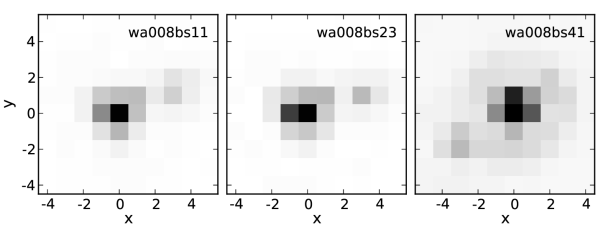
The separation between the centers of WASP-8A and WASP-8B in the IRAC detectors is only 3.7 pixels. Consequently, the signal from the stars overlapped, demanding special care during the data analysis (see Figure 1). Table 2 shows the average and standard deviation of the flux ratio, separation, and position angle (PA) of the secondary star with respect to WASP-8A (derived from our centering routine, see Section 3.2). Our PA values agree with those of Queloz et al. (2010), but our separation values are consistently lower than theirs ($4.83{\arcsec}\pm 0.01$″).

Table 2 WASP-8 System

Event	deFlux ratio		Separation (pixels)		Separation (″)		Position angle (deg)
	average	stddev	average	stddev	average	stddev	average	stddev
wa008bs11	0.1420	0.0030	3.760	0.013	4.610	0.016	171.32	0.28
wa008bs21	0.1512	0.0017	3.734	0.007	4.541	0.009	171.00	0.15
wa008bs22	0.1600	0.0022	3.737	0.009	4.544	0.011	170.75	0.16
wa008bs23	0.1648	0.0039	3.726	0.017	4.497	0.020	170.78	0.29
wa008bs41	0.1718	0.0020	3.690	0.009	4.513	0.011	170.84	0.17
wa008bs42	0.1794	0.0023	3.686	0.010	4.506	0.012	170.96	0.16

3. Data Analysis

Our Photometry for Orbits, Eclipses, and Transits (POET) pipeline produces light curves from BCD images. Briefly, POET creates a bad pixel mask for each image, finds the center position of the target, executes interpolated aperture photometry, and fits a light curve model that includes physical and systematic parameters.

3.1. POET: Initial Reduction

POET created bad pixel masks by discarding the flagged pixels from the Spitzer BCD masks. Then, it discarded outlier pixels with a sigma-rejection method. At each pixel position and in sets of 64 consecutive images, POET calculated the median and standard deviation of the unmasked pixels. Pixels diverging more than four times the standard deviation from the median were masked. We iterated this process twice.

We obtained the Julian Date of each frame from the UTCS_OBS and FRAMTIME entries of the files’ headers. We calculated the Barycentric Julian Date (BJD) by correcting the projected light-travel time from the telescope to the Solar System’s barycenter using the Jet Propulsion Laboratory (JPL) Horizons system. We report the times in both Coordinated Universal Time (UTC) and the Barycentric Dynamical Time (TDB); the latter is unaffected by leap seconds (Eastman et al., 2010).

3.2. Centering

POET provides three routines to determine the center of the point-spread function (PSF) in each image: center of light, 2D-Gaussian fitting, and least asymmetry (Stevenson et al., 2010, Supplementary Information). The proximity of WASP-8B confuses these methods, so we added a double-PSF fit that shifts supersampled PSFs to the target and secondary, bins them down, and scales their amplitudes, as in Crossfield et al. (2010). For each Spitzer band we used Tiny Tim (version 2.0) to create a stellar PSF model with a 5600 K blackbody spectrum at 100$\times$ finer resolution than our images. The double-PSF routine has seven free parameters: the position of each star ($x_{A}$, $y_{A}$, $x_{B}$, $y_{B}$), the integrated stellar fluxes ($F_{A}$, $F_{B}$), and the background sky flux ($f$sky).

To avoid interpolation when binning down, the PSF shifts are quantized at the model’s resolution, such that image and model pixel boundaries coincide. This quantization sets the position precision to 0.01 pixels. It also excludes the position parameters from $\chi^{2}$ minimizers that assume a continuous function, such as Levenberg-Marquardt. So, we fit $F_{A}$, $F_{B}$, and $f$sky for a given position set x $=\{x_{A}$, $y_{A}$, $x_{B}$, $y_{B}\}$.

To avoid the computational challenge of performing a $\chi^{2}$ minimization for each x in a 4D space at 0.01 pixel resolution, we explored only specific coordinate positions. Starting at an initial guess position, and with an initial jump step of 100 positions (1 image pixel), we calculated $\chi^{2}$ at that position and the 80 ($=3^{4}-1$) adjacent positions that are one jump step away along all combinations of coordinate directions. We either moved to the lowest $\chi^{2}$or, if already there, shrank the step by half. We repeated the procedure until the step was zero.

3.3. Photometry

Circular aperture photometry is unsuitable for this system, since any flux from the secondary star (WASP-8B) contained in the aperture dilutes the eclipse depth of WASP-8b. Small pointing jitter would also increase the light-curve dispersion for any aperture that included much WASP-8B flux. Apertures that are too large or small both produce noisier light curves. Thus, we modified the POET interpolated aperture photometry (Harrington et al., 2007, Supplementary Information) to remove the secondary star two different ways. In both methods, we subtracted the median sky level prior to the stellar flux calculation. The sky annulus included values 7 – 15 pixels from the target.

In our first method (B-Subtract), we subtracted the fitted, binned PSF model of WASP-8B from each image. Then, we performed interpolated aperture photometry centered on the target (A aperture). In the second method (B-Mask), we discarded the pixels within a circular aperture centered at the position of the secondary before performing aperture photometry. The mask’s aperture must encompass most of the contribution from WASP-8B, but not from the target. Therefore, we tested mask apertures with 1.6, 1.8, and 2.0 pixel radii. For each photometry method we tested a broad range of A-aperture radii in 0.25 pixel intervals.

The B-Mask method has less residual dispersion when the mask is located at a fixed vector separation from WASP-8A (using the median of all the measured separations in an event), than when its position is determined for each individual frame. This can be explained by the dimmer signal of WASP-8B, which lowers the accuracy of its position estimation. So, within each data set using B-Mask, we used the median vector separation of the two objects. For the B-subtract method, the standard deviation of the normalized residuals (SDNR) and eclipse-depths differences are marginal.

3.4. Light Curve Modeling

The eclipse depths of WASP-8b are on the order of 0.1% of the system’s flux, well below Spitzer’s photometric stability criteria (Fazio et al., 2004). Thus, the eclipse light-curve modeling requires a thorough characterization of the detector systematics. Systematic effects have been largely observed and documented; they can have both temporal and spatial components, and vary in strength and behavior for each data set.

The main systematic at 3.6 and 4.5 m is intrapixel sensitivity variation, $M(x,y)$, where the measured flux depends on the precise position of the target on the array (Stevenson et al., 2012; Charbonneau et al., 2005). In addition, the detectors show a time-dependent sensitivity variation called the ramp effect, $R(t)$, suspected to be caused by charge trapping (Agol et al., 2010) at 8.0 m, but there are also reports of a ramp in the 3.6 and 4.5 m bands (e.g., Campo et al., 2011; Nymeyer et al., 2011; Knutson et al., 2011; Deming et al., 2011; Blecic et al., 2013; Stevenson et al., 2010, 2012). The eclipse and both systematic variations entangle to produce the observed light curve. To account for their contributions, we modeled the light curves as

$$F(x,y,t)=F_{s}M(x,y)R(t)E(t),$$ (1)

where $F_{s}$ is the out-of-eclipse system flux. We used the eclipse model, $E(t)$, from Mandel & Agol (2002). The eclipse is parametrized by the eclipse depth, the mid-point phase, the duration, and the ingress and egress times. For the ingress/egress times we adopted a value of 18.8 min, derived from the orbital parameters of the planet. We used this value in all of our eclipse-model fits.

The strength and behavior of the ramp variations are specific to each dataset. Many formulae have been applied in the literature (e.g., Deming et al., 2007; Harrington et al., 2007; Knutson et al., 2011; Stevenson et al., 2012). The models are formed with combinations of exponential, logarithmic, and polynomial functions. We tested dozens of equations; the best were:

$${\rm risingexp}:\quad R(t) = 1-e^{-r_{0}(t-t_{0})}$$ (2)

$${\rm logramp}_{q}:\quad R(t) = 1+r_{q}[\ln(t-t_{0})]^{q}$$ (3)

$${\rm linramp}:\quad R(t) = 1+r_{1}(t-t_{c})$$ (4)

$${\rm quadramp}_{1}:\quad R(t) = 1+r_{1}(t-t_{c})+r_{2}(t-t_{c})^{2}$$ (5)

$${\rm quadramp}_{2}:\quad R(t) = 1+r_{2}(t-t_{c})^{2}$$ (6)

$${\rm loglinear}:\quad R(t) = 1+r_{1}(t-t_{c})+r_{4}\ln(t-t_{0})$$ (7)

where $t_{c}$ is a constant value at the approximated mid-point phase of the eclipse ($t_{c}=0.515$ for this planet). Slight changes in $t_{c}$ do not significantly affect the fitted eclipse parameters.

We used our Bi-Linearly Interpolated Subpixel Sensitivity (BLISS) mapping technique (Stevenson et al., 2012) to calculate $M(x,y)$. The BLISS method has been found to return a better result than a polynomial fit (Stevenson et al., 2012; Blecic et al., 2013).

To determine the best-fitting parameters of our model, Equation (1), we used a $\chi^{2}$ minimizer with the Levenberg-Marquardt algorithm. We used Bayesian posterior sampling via an MCMC algorithm to explore the phase space and estimate the uncertainties of the free parameters of the light-curve models. Our code implements the Metropolis random walk, which proposes parameter sets from a multivariate normal distribution centered at the current position in the chain, computes $\chi^{2}$, and accepts (or rejects) the new set with greater probability for a lower (higher) $\chi^{2}$. By generating millions of parameters sets, the algorithm samples the posterior distribution of the model parameters. As a necessary condition for chain convergence, we require the Gelman-Rubin statistic (Gelman & Rubin, 1992) to be within 1% of unity for each free parameter between four MCMC chains.

The photometry routine uses the BCD uncertainty images to estimate the uncertainties of the light-curve data points, $\sigma_{i}$. However, since the Spitzer pipeline in general overestimates these uncertainties (it is designed for absolute photometry), we multiply by a constant factor ($\sigma_{i}\rightarrow f\cdot\sigma_{i}$), such that the reduced $\chi^{2}=1$ in the light-curve fit. This is equivalent to estimating a single $\sigma$ from the scatter of model residuals. Both methods account for red noise, but ours retains the (usually small) $\sigma_{i}$ variations due to aberrant frames.

To determine the best raw light curve (i.e., by selection of photometry method and aperture radius), we calculated the SDNR of the light-curve fit (Stevenson et al., 2012; Campo et al., 2011). Poor fits or data with high dispersion increase SDNR; the optimum data set minimizes the SDNR value. Once we chose the best light curve, we compared the different ramp models according to the Bayesian Information Criterion (Liddle, 2007),

$${\rm BIC}=\chi^{2}+k\ln N,$$ (8)

where $k$ is the number of free parameters and $N$ the number of data points. The best model minimizes the BIC. The probability ratio favoring one model over a second one is $\exp(-\Delta{\rm BIC}/2)$.

3.4.1 wa008bs11 Analysis

This observation started 2.9 hours before the eclipse’s first contact. The telescope observed the target in sub-array mode, allowing a high cadence (Table 1). We discarded the initial 15 minutes of observation while the telescope pointing settled. Our data present both intrapixel and weak ramp systematics.

Figure 2.— Raw (left), binned (center) and systematics-corrected (right) secondary-eclipse light curves of WASP-8b at 3.6, 4.5, and 8.0 m. The system flux is normalized to unity and the points are shifted vertically for clarity. The colored curves are the best-fit models (see legend). The black curves are the best-fit models excluding the eclipse component. The error bars in the center and right panels are the 1$\sigma$ uncertainties.

Table 3 wa008bs11 Ramp Model Fits

$R(t)$	SDNR	$\Delta$BIC	Ecl. Depth (%)
quadramp1	0.0061141	0.00	0.119
risingexp	0.0061148	1.73	0.106
logramp1	0.0061153	2.96	0.096
linramp	0.0061201	6.34	0.063
loglinear	0.0061141	11.10	0.119

The 2.25 pixel A aperture with B-subtract photometry minimized SDNR. Table 3 shows the five best-fitting models to the best wa008bs11 light curve. $\Delta$BIC is with respect to the lowest BIC value. The quadramp1 model is 2.4 times more probable than, and consistent with, the second-best model. The linear ($11\sigma$) and and quadratic ($4\sigma$) terms of the quadramp1 model (see Table 9) confirm the need for a ramp model. As a general remark, we noted that all the logrampq models produce similar BIC and eclipse parameter values; therefore, we will refer only to the logramp1 model in the future. Models with more free parameters do not improve BIC. Following Stevenson et al. (2012), we vary the bin size and the minimum number of data points per bin (mnp) of the BLISS map to minimize the dispersion of the residuals. We required at least 4 points per bin for any dataset. The PSF-fitting position precision of 0.01 pixels sets our lower limit for the binsize. For wa008bs11, $mnp=5$ and a bin size of 0.015 pixels optimized the fit.

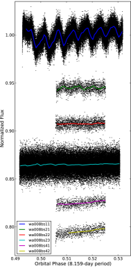
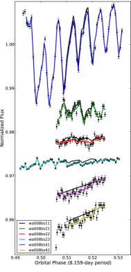
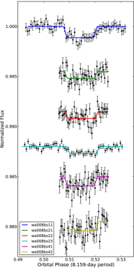
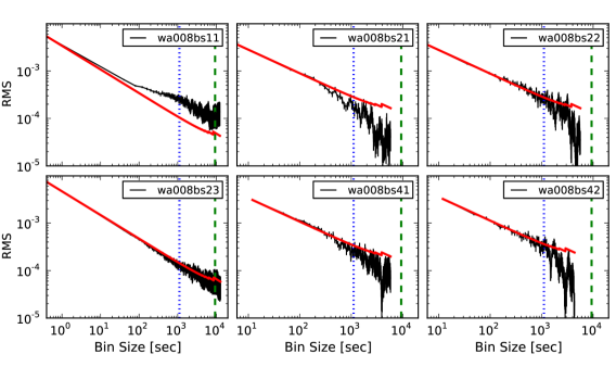
Figure 2 shows the raw, binned and systematics-corrected wa008bs11 light curves with their best-fitting model. We considered the correlated noise in the residuals as well (Pont et al., 2006). Figure 3 shows the root-mean-square (RMS) of the residuals vs. bin size. The wa008bs11 RMS curve deviates above the expected RMS for pure Gaussian noise. Following Winn et al. (2008), to account for the correlated noise, we weighted the light curve uncertainties by the factor $\beta$ (the fractional RMS excess above the pure Gaussian RMS at the bin size corresponding to the eclipse duration). For wa008bs11 we found $\beta=2.4$. We inspected all the pairwise correlation plots and histograms and found only unimodal Gaussian distributions.

Alternatively, the residual-permutation (also known as prayer bead) algorithm is sometimes used to assess correlated noise in a fit. In this method, we cyclically shift the residuals from the best model by one frame, add them back to that model, and re-fit, repeating until we shift the residuals back to their original positions. This generates a distribution of values for each parameter, from which we estimate the parameter uncertainties. The eclipse-depth uncertainty is 0.021%, similar to the value found with the Winn et al. (2008) method (see Table 9). However, we are cautious. Although prayer bead has been broadly used for the analysis of exoplanet lightcurve and RV fits (e.g., Southworth, 2008; Bouchy et al., 2005; Pont et al., 2005; Gillon et al., 2007; Knutson et al., 2008; Cowan et al., 2012), we have found no detailed description of its statistical properties in the literature.

Figure 3.— RMS of the fit residuals (black curves with 1$\sigma$ uncertainties) vs.  bin size of the WASP-8b light curves. The red curves are the expected RMS for Gaussian noise (extrapolated unbinned RMS scaling by the inverse square root of the bin size). The blue dotted and green dashed vertical lines mark the bin size corresponding to the eclipse ingress and duration time, respectively. wa008bs11’s excess above the red line indicate correlated noise at bin sizes larger than the ingress time.

3.4.2 wa008bs23 Analysis

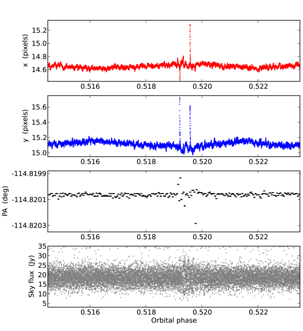
With the same observing setup as wa008bs11, this observation started 3.3 hours prior to the eclipse’s first contact. This dataset also presented both intrapixel and ramp variations. Note that the intrapixel systematic is weaker than at 3.6 m, attributed to the smaller degree of undersampling at larger wavelengths by Charbonneau et al. (2005) and Morales-Calderón et al. (2006). Even though the pointing stabilized only after the initial 20 minutes, the light curve did not deviate significantly; therefore, we included all data points in the analysis. We noted two sudden pointing and PA deviations near phase 0.519. After each incident, the telescope resumed its position within $\sim$10 s (Figure 4). Micrometeorite impacts on the telescope can explain the abrupt deviations. Simultaneously, we measured a slight increase in the background sky flux dispersion, which returned to normality shortly after. The target flux did not show any extraordinary fluctuations during these incidents. However, the points outside the normal pointing range were eliminated by the BLISS map’s mnp criterion.

Figure 4.— wa008bs23 target pointing, position angle and background sky flux near phase 0.519. We observed two sudden position shifts coincident with increases in the background flux. All values returned to normal almost instantly.

The analysis is analogous to wa008bs11. The SDNR indicated clearly that the 2.25 pixel A aperture with B-Subtract photometry produced the lowest dispersion. The best-fitting ramp model is logramp1, which is 21 times more probable than the rising exponential ramp (Table 4). The BLISS map is optimized at $mnp=4$ and a bin size of 0.025 pixels.

An initial MCMC run showed a significant linear correlation between the system flux and the $r_{1}$ parameter of the logramp, which prevented the MCMC chain from converging. We solved this problem by transforming the correlated parameters into an orthogonal set of parameters, rerunning the MCMC chain, and inverting the transformation on the resulting parameter values (Stevenson et al., 2012). Figures 2 and 3 show the wa008bs23 light curves with the best-fitting model and RMS of the residuals vs. bin size.

Table 4 wa008bs23 Ramp Model Fits

$R(t)$	SDNR	$\Delta$BIC	Ecl. Depth (%)
logramp1	0.0073830	0.00	0.0677
risingexp	0.0073832	6.10	0.0730
quadramp1	0.0073833	9.40	0.0777
loglinear	0.0073830	10.84	0.0685
linramp	0.0073846	12.19	0.0564

3.4.3 wa008bs21 & wa008bs41 Analysis

We simultaneously observed wa008bs21 and wa008bs41 in full-array mode. Prior to the eclipse observation, we exposed the detector (a “preflash” observation, Knutson et al., 2009) for 25 minutes to a bright H II region, with coordinates $\alpha~{}=~{}20$h 21m 39s.28 and $\delta~{}=~{}+37$° 31′ 03.6″, to minimize the ramp systematic variation. The secondary-eclipse observation started only 26 minutes before the first contact. The telescope pointing stabilized quickly, so fortunately we needed to remove only the initial four minutes of observation. Every 12 s, the detector recorded two consecutive images (two-second exposures) at 4.5 m and one image at 8.0 m. (Table 1).

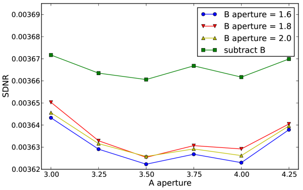
The SDNR analysis of wa008bs21 showed that a 3.5 pixel A aperture with 1.6 pixel B-Mask photometry minimizes the dispersion (Figure 5). The ramp models indicated a negligible ramp variation. Accordingly, a fit without a ramp model yielded the lowest BIC. Table 5 shows the four best-fitting models for the best wa008bs21 data set. The no-ramp model is 15 times more probable than the quadramp2 model.

Figure 5.— wa008bs21 Standard Deviation of the Normalized Residuals vs. aperture (in pixels). The SDNR curves use the best ramp model in Table 5. The legend indicates the photometry method. SDNR increases at 3.75 pixels (coincident with the stars’ separation). The eclipse parameters are consistent over the 3.0–4.25 aperture range. The optimum dataset uses 1.6 pixel B-Mask photometry with a 3.5 pixel A aperture.

Table 5 wa008bs21 Ramp Model Fits

$R(t)$	SDNR	$\Delta$BIC	Ecl. Depth (%)
no ramp	0.0036223	0.00	0.0718
quadramp2	0.0036195	5.76	0.1189
linramp	0.0036223	7.56	0.0714
quadramp1	0.0036197	13.14	0.1170

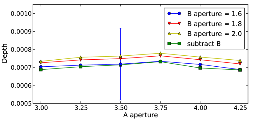
Because of the shorter out-of-eclipse observation, the system flux is less-constrained for wa008bs21 than for the wa008bs11 or wa008bs23 events. Combined with a correlation between the eclipse depth and system flux (revealed by MCMC), the lower precision of the system flux translates into a larger eclipse depth uncertainty. Nevertheless, the wa008bs21 fit parameters were consistent among the different apertures (Figure 6). The optimum parameters of the BLISS map are $mnp=5$ and a bin size of 0.025 pixels.

Figure 6.— Eclipse depth vs. A aperture for wa008bs21. Each color represent a different photometry method as in Figure 5. The blue error bar corresponds to the 1-$\sigma$ uncertainty of the best model. The eclipse duration and mid-point phase follow a similar trend.

The 8.0 m detector did not present an intrapixel pattern like the 3.6 or 4.5 m detectors. However, some of the raw light curves for different apertures and photometry methods showed large scatter and presented strong oscillations, producing implausible fit parameters. A pixelation effect (Anderson et al., 2011; Stevenson et al., 2012) might be responsible. As a consequence, we were unable to fit the eclipse parameters unambiguously for this data set alone. Normally we study the events individually to select the best aperture and photometry method, but in this case we used a joint fit with the best wa008bs21 dataset and model to help constrain the 8.0 m eclipse curve, sharing the eclipse duration and mid-point parameters. The 3.5 pixel A aperture with 1.6 pixel B-mask photometry for wa008bs41 minimized the joint SDNR (Figure 7).

Figure 7.— Joint wa008bs21+wa008bs41 Standard Deviation of the Normalized Residuals vs. aperture radius (in pixels) of wa008bs41, for different photometry methods. All 24 light curves use the best ramp model from Table 6. Light curves using 1.6 and 2.0 pixel B-Mask photometry at 3.5 pixel A aperture produce consistent eclipse parameters and outperform the best B-subtract method (with a 3.75 pixel A aperture). The best B-subtract also yields a more scattered raw light curve. Hence, the optimum dataset uses 1.6 pixel B-mask photometry with a 3.5 pixel A aperture.

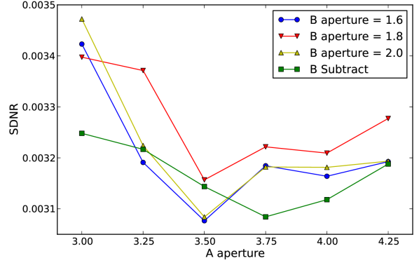
Table 6 compares the four best-fitting ramp models for the best wa008bs41 light curve. A linear ramp minimizes BIC, and is 20 times more probable than the next-best model. Figures 2 and 3 show the wa008bs21 and wa008bs41 light curves with their best-fitting models and RMS of the residuals vs. bin size, respectively.

Table 6 wa008bs41 Ramp Model Fits

R(t)	SDNR 4&2	$\Delta$BIC	Ecl. Depth (%)
linramp	0.0030766	0.00	0.0931
quadramp1	0.0030744	5.94	0.1308
risingexp	0.0030754	6.33	0.1150
logramp1	0.0030758	6.50	0.1078

3.4.4 wa008bs22 & wa008bs42 Analysis

The observing setup of these events was identical to wa008bs21 and wa008bs41, including the preflash observation. The pointing of this observation drifted noticeably more than in the other observations, moving more than $0.4$ pixels during the initial 30 minutes and stabilizing only during the eclipse. As a consequence, the illumination level of the individual pixels changed during the beginning of the eclipse. The ramp variation, which depends on the illumination (Knutson et al., 2008), was disrupted.

The wa008bs22 event, having a negligible ramp variation, was little affected by the telescope pointing shift. The SDNR calculation for wa008bs22 indicated the 1.8 pixel B-Mask photometry with 3.75 pixel A aperture as the best dataset. A light-curve model without a ramp (Table 7) is 639 times more probable than the quadramp2 model. The optimal BLISS map has $mnp=4$ and a bin size of 0.02 pixels.

Table 7 wa008bs22 Ramp Model Fits

$R(t)$	SDNR	$\Delta$BIC	Ecl. Depth (%)
no ramp	0.0025274	0.00	0.0814
quadramp2	0.0025253	12.94	0.1224
logramp1	0.0025267	14.22	0.0921
risingexp	0.0025274	15.04	0.0814

In contrast, we discarded the initial wa008bs42 light curve past the eclipse ingress due to the disrupted ramp variation. The eclipse model parameters are thus less constrained. By this point, we already had single-channel fits for the rest of the data, so we tuned the wa008bs42 analysis in a joint fit with all the other events, sharing the eclipse duration and mid-time. SDNR indicates the B-subtract method with 4.00 pixel A aperture as the best dataset. Table 8 presents the four best-fitting models. The eclipse depth is consistent with the wa008bs41 depth.

Table 8 wa008bs42 Ramp Model Fits

R(t)	SDNR	$\Delta$BIC	Ecl. Depth (%)
linramp	0.0032320	0.00	0.0932
quadramp1	0.0032312	6.19	0.0892
logramp1	0.0032321	6.67	0.0938
risingexp	0.0032330	7.08	0.0961

3.4.5 Final Joint-fit Analysis

Table 9 Best-Fit Eclipse Light-Curve Parameters

Parameter	wa008bs11	wa008bs21	wa008bs22	wa008bs23	wa008bs41	wa008bs42
Array Position ($\bar{x}$, pix)	14.74	20.76	20.39	14.65	19.11	18.72
Array Position ($\bar{y}$, pix)	15.07	233.30	233.30	15.12	230.27	230.20
Position Consistency ($\delta_{x}$, pix)	0.0072	0.0223	0.0220	0.0097	0.0273	0.0254
Position Consistency ($\delta_{y}$, pix)	0.0118	0.0228	0.0236	0.0101	0.0272	0.0274
A Aperture Size (pix)	2.25	3.5	3.75	2.25	3.5	4.0
WASP-8B photometric correction	subtract	1.6 mask	1.8 mask	subtract	1.6 mask	subtract
System Flux $F_{s}$ (Jy)	144555.0(21.0)	91369.9(8.5)	90850.3(8.5)	87473.0(21.0)	32892.5(6.6)	34949.8(8.9)
Eclipse Depth (%)	0.113(18)	0.0692(68)	0.0692(68)	0.0692(68)	0.093(23)	0.093(23)
Brightness Temperature (K)	1552(85)	1131(35)	1131(35)	1131(35)	938(99)	938(99)
Eclipse Mid-point (orbits)	0.51428(34)	0.51446(37)	0.51468(41)	0.51536(28)	0.51446(37)	0.51468(41)
Eclipse Mid-point (MJDUTC)	5401.4981(28)	4822.2301(31)	4814.0732(33)	5409.6656(23)	4822.2301(31)	4814.0732(33)
Eclipse Mid-point (MJDTDB)	5401.4989(28)	4822.2309(31)	4814.0739(33)	5409.6663(23)	4822.2309(31)	4814.0739(33)
Eclipse Duration ($t_{\rm 4-1}$, hrs)	2.600(78)	2.600(78)	2.600(78)	2.600(78)	2.600(78)	2.600(78)
Ingress/Egress Time ($t_{\rm 2-1}$, hrs)	0.314	0.314	0.314	0.314	0.314	0.314
Ramp Equation ($R(t)$)	quadramp1	None	None	logramp1	linramp	linramp
Ramp, Linear Term ($r_{1}$)	0.0707(70)	—	—	0.000504(45)	0.205(22)	0.246(37)
Ramp, Quadratic Term ($r_{2}$)	$-$3.17(75)	—	—	—	—	—
Ramp, Phase Offset ($t_{0}$)	—	—	—	0.4917	—	—
BLISS Map ($M(x,y)$)	Yes	Yes	Yes	Yes	No	No
Minimum number of Points Per Bin	5	5	4	4	—	—
Total Frames	64320	2024	2024	64320	1012	1012
Frames Used	62203	1936	1879	64072	966	725
Rejected Frames (%)	3.29	4.35	7.16	0.39	4.54	28.36
Free Parameters	6	4	4	5	5	5
BIC Value	80444.5	80444.5	80444.5	80444.5	80444.5	80444.5
SDNR	0.0053772	0.0036250	0.0035698	0.0073926	0.0030768	0.0032320
Uncertainty Scaling Factor	0.3075	1.0280	1.0077	1.0902	1.1187	1.1382
$\beta$ correction	2.4	—	—	—	—	—
Photon-Limited S/N (%)	37.00	94.71	96.59	89.66	76.94	71.00

Notes: The values quoted in parenthes are the 1$\sigma$ uncertainties.

From the three individual fits to the 4.5 m observations we found eclipse depths of $0.072\%\pm 0.021\%$, $0.086\%\pm 0.022\%$, and $0.068\%\pm 0.007\%$ for wa008bs21, wa008bs22, and wa008bs23, respectively. The weighted mean of the depths is $0.0692\%\pm 0.0065\%$. With a dispersion of 0.0062% around the mean, this is not larger than the individual uncertainties, thus we found no evidence for temporal variability. This dispersion corresponds to 10% of the mean eclipse depth. The consistency permitted a joint analysis of all observations. We used the best light curves and models found in the individual fits, where all events shared the eclipse duration, the three 4.5-m events shared their eclipse depth, the two 8.0-m events shared their eclipse depth, the simultaneous wa008bs21 and wa008bs41 events shared their eclipse mid-point phases, and the wa008bs22 and the wa008bs42 events shared their eclipse mid-point phases. Table 9 shows the light-curve modeling setup and results. We used these joint-fit results for the orbital and atmospheric analysis. An electronic supplement contains the best light curves, including centering, photometry, and the joint fit.

4. Orbital Dynamics

WASP-8b’s high eccentricity ($e=0.31$) implies that its separation from WASP-8A at periapsis (0.055 AU) is about half that at apoapsis. Given the argument of periapsis ($\omega=-85.86\arcdeg$), the secondary eclipse nearly coincides with the periapsis. The planet, therefore, receives over twice as much flux at eclipse as it would if the orbit were circular, explaining in part our high brightness temperature (see Table 9).

Secondary-eclipse times can refine estimates of $e\cos\omega$ from RV data. The four eclipse events occurred at an average eclipse phase of $0.514695\pm 0.00018$. After subtracting a coarse light-time correction of $2a/c=80$ s from this average phase, we calculated $e\cos\omega=0.02290\pm 0.00028$ (see Equation (3) of Charbonneau et al., 2005). This is consistent with Queloz et al. (2010), and photometrically confirms the nonzero eccentricity of the planet’s orbit (we fit $e\cos\omega$ below without relying on the low $e$ approximation).

The eclipse timings were combined with 130 available RV data points and with transit data from Queloz et al. (2010) using the method described by Campo et al. (2011) and Nymeyer et al. (2011). Forty-eight in-transit RV points were removed due to the Rossiter-McLaughlin effect.

Our fit presented a moderate improvement to the orbital parameters of WASP-8b (Table 10), except for the period. While Queloz et al. (2010) used several transits to measure the period, we used their published mid-point epoch (a single date); hence, our period is constrained mostly by our eclipses and the RV data, and thus have a larger uncertainty. By themselves, the secondary eclipses have a period of $8.158774\pm 0.00040$ days and a midpoint epoch of BJD $2455409.6629\pm 0.0017$ (TDB), not significantly ([$5.9\pm 4.3]\times 10^{-5}$ days) longer than the period found by Queloz et al. (2010). The transit and eclipse periods place a $9.8\times 10^{-5}$ ° day^-1 ($3\sigma$) upper limit on possible apsidal precession, nearly three orders of magnitude larger than the theoretical expectation for tidal effects (Ragozzine & Wolf, 2009).

Table 10 Eccentric Orbital Model

Parameter	This work		Queloz et al. (2010)
$e\sin\omega$	$-0.3078$ $\pm$	0.0020	$-0.3092$ $\pm$	0.0029
$e\cos\omega$	$0.02219$ $\pm$	0.00046	$0.023$ $\pm$	0.001
$e$	0.309 $\pm$	0.002	0.310 $\pm$	0.0029
$\omega$ (°)	$-85.00$ $\pm$	0.08	$-85.73$ $\pm$	0.18
$P$ (days)	8.158719 $\pm$	0.000034	8.158715 $\pm$	0.000016
$T_{0}$ (MJDTDB)	4679.33486 $\pm$	0.00057	4679.33509 $\pm$	0.00050
$K$ (ms-1)	221.9 $\pm$	0.6	222.23 $\pm$	0.8
$\gamma_{C}$ (ms-1)	$-1\,565.9$ $\pm$	0.6	$-1\,565.8$ $\pm$	0.21
$\gamma_{H}$ (ms-1)	$-1\,547.4$ $\pm$	0.4	$-1\,548.1$ $\pm$	0.6
$\dot{\gamma}$ (ms-1yr-1)	$58.1$ $\pm$	1.2	$58.1$ $\pm$	1.3
Reduced $\chi^{2}$	4.1		0.86

5. Atmospheric Analysis

Figure 8.— Left: Atmospheric spectral emission of the dayside of WASP-8b. The blue circles with error bars are the measured eclipse depths, or equivalently, the planet-star flux ratios. The red and green curves show two model spectra with the same temperature profile (shown in the inset) but with different compositions. The green curve shows a model assuming chemical equilibrium with solar elemental abundances. The red curve shows a model with $10^{3}$ times lower methane abundance compared to the green model, but the abundances of the remaining molecules are identical to those in the green model. The red and green filled circles are the corresponding model fluxes integrated over the Spitzer bands (bottom solid lines). The black dashed lines represent planetary blackbody spectra with $T=710,1100$, and 1450 K. Right: Normalized contribution functions of the solar-composition model (solid lines) and the low-CH4-abundance model (dotted lines) in each Spitzer band (see legend). The effective pressures of the contribution functions are 0.63, 0.35, and 0.12 bar at 3.6, 4.5, and 8.0 m, respectively.

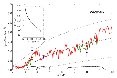
We use our IRAC observations of thermal emission from WASP-8b to constrain the thermal structure and composition of the dayside atmosphere of the planet. The Spitzer bandpasses at 3.6, 4.5, and 8.0 m contain strong spectral features due to several carbon and oxygen-based molecules that are expected in hot-Jupiter atmospheres. Methane (CH4) has strong spectral features in the 3.6 and 8.0 m bands, carbon monoxide (CO) and carbon dioxide (CO2) have features at 4.5 m, while water vapor (H2O) has features in all three bands (Madhusudhan & Seager, 2010). The spectral features of the various molecules appear as absorption troughs or emission peaks in the emergent spectrum depending on whether the temperature decreases or increases with altitude, respectively. Consequently, strong degeneracies exist between the temperature structure and molecular composition derived from a spectral dataset (e.g., Madhusudhan & Seager, 2010). Nevertheless, photometric observations made with Spitzer have been successfully used to constrain chemical compositions and temperature structures in many exoplanetary atmospheres (e.g., Barman et al., 2005; Burrows et al., 2007; Knutson et al., 2008; Madhusudhan & Seager, 2009; Stevenson et al., 2010; Madhusudhan et al., 2011).

We model the dayside emergent spectrum of WASP-8b using the atmospheric modeling and retrieval method of Madhusudhan & Seager (2009, 2010). The model computes line-by-line radiative transfer in a plane-parallel atmosphere assuming hydrostatic equilibrium, local thermodynamic equilibrium, and global energy balance. We assume a Kurucz model for the stellar spectrum (Castelli & Kurucz, 2004) given the stellar parameters. The pressure-temperature ($P$–$T$) profile and molecular mixing ratios are free parameters in the model, which can be constrained from the data. The $P$–$T$ profile comprises of six free parameters and the mixing ratio of each molecular species constitutes an additional free parameter. Following Madhusudhan & Seager (2009), we parametrize the mixing ratio of each species as deviations from thermochemical equilibrium assuming solar elemental abundances (Burrows & Sharp, 1999). We include the dominant sources of opacity expected in hot Jupiter atmospheres, namely molecular absorption due to H2O, CO, CH4 and CO2 (Freedman et al., 2008; R.S. Freedman 2009, private communication), and H₂-H₂ collision induced absorption (Borysow, 2002). We explore the model parameter space in a Bayesian way using an MCMC sampler (Madhusudhan & Seager, 2010, 2011). Given the limited number of observations ($N_{\rm obs}$=3), our goal is not to find a unique model fit to the data; instead, we intend to constrain the region of atmospheric parameter space that is allowed or ruled out by the data.

Our observations rule out a thermal inversion in the dayside atmosphere of WASP-8b. This is evident from the planet–star flux contrasts in the three IRAC bands at 3.6, 4.5, and 8.0 m. In the presence of a thermal inversion, the planet–star flux contrasts in the 4.5 and 8.0 m bands are both expected to be greater than the flux contrast in the 3.6 m band (Burrows et al., 2008; Fortney et al., 2008; Madhusudhan & Seager, 2010), due to spectral features of the dominant molecules appearing as emission peaks as opposed to absorption troughs. However, the low 4.5 and 8.0 m flux contrasts relative to the 3.6 m contrast requires significant absorption due to H₂O and CO across the spectrum, and hence the lack of a thermal inversion in the atmosphere. Figure 8 shows model spectra of WASP-8b with no thermal inversion in the temperature profile. The observed 4.5 and 8.0 m flux contrasts are explained to a good level of fit by a model without a thermal inversion and with solar abundance composition, as shown by the green curve in Figure 8. Our inference of the lack of a thermal inversion in WASP-8b is independent of any assumption about chemical composition or C/O ratio (e.g. Madhusudhan & Seager, 2011). The lack of a thermal inversion in WASP-8b is not surprising, since it is amongst the cooler population of irradiated hot Jupiters, which are not expected to host inversion-causing species such as TiO or VO in their upper atmosphere (Fortney et al., 2008; Spiegel et al., 2009).

Our models are unable to reproduce the high planet–star flux contrast observed in the 3.6 m IRAC band, independent of the composition. The major sources of absorption in the 3.6 m band are H2O and CH4. In principle, decreasing the CH4 and/or H2O abundances can lead to a higher 3.6 m contrast. However, as shown by the red curve in Figure 8, such an increase also simultaneously increases the contrast in the 8.0 m band, thereby worsening the fit overall. Another hindrance to fitting the observed 3.6 m contrast is that it requires a hotter $P$–$T$ profile, with $T\gtrsim$ 1550 K in the lower atmosphere, predicts much higher fluxes in the 4.5 and 8.0 m bands than observed. On the other hand, a cooler $P$–$T$ profile than shown in Figure 8 would provide a better fit in the 4.5 and 8.0 m bands, but would further worsen the fit in the 3.6 m band. Consequently, we choose an intermediate $P$–$T$ profile that provides a compromise fit to all three data points.

Although the one-dimensional (1D) models shown in Figure 8 output less energy than the instantaneous incident irradiation during the eclipse (concurrent with periastron passage), they output $\sim$ 20% higher energy compared to the time-averaged incident irradiation received at the substellar point. Considering that a pseudo-synchronous rotation should facilitate the redistribution of energy to the night side, the high emission measured suggests that WASP-8b is quickly reradiating the incident irradiation on its dayside hemisphere, i.e. nearly zero day–night redistribution. Such a scenario would lead to a large day–night temperature contrast in the planet which can be confirmed by thermal phase curves of the planet observed using warm Spitzer (e.g., Knutson et al., 2009). The high emergent flux also implies a very low albedo, as with most hot-Jupiter planets (Cowan & Agol, 2011b).

6. The Unexpected Brightness Temperatures of WASP-8b

As seen in the previous section, the 3.6-m brightness temperature is anomalously higher than expected. The hemisphere-averaged equilibrium temperature for instantaneous reradiation (time-averaged around the orbit) is only 948 K; even the instantaneous equilibrium temperature at periapsis, 1128 K, is far lower than this observation. Thus, we modeled the orbital thermal variation due to the eccentricity to determine if such a high temperature is possible from irradiation alone.

Following Cowan & Agol (2011a), we solved the energy balance equation in a one-layer latitude–longitude grid over the planetary surface. The change in temperature of a cell with time, ${{\mathrm{d}}T}/{{\mathrm{d}}t}$, is determined by the difference between the absorbed flux from the star and the re-emitted blackbody flux,

$$\frac{{\rm d}T}{{\rm d}t}=\frac{1}{c_{h}}\left[(1-A)\sigma T^{4}_{\rm eff}\left(\frac{R_{*}}{r(t)}\right)^{2}\cos\psi(t)\ -\ \sigma T^{4}\right],$$ (9)

where $c_{h}$ is the heat capacity per unit area; $T_{\rm eff}$ and $R_{*}$ are the star’s effective temperature and radius, respectively; $r(t)$ is the planet–star separation; $\cos\psi(t)=\sin\lambda\,{\rm max}(\cos\Phi(t),0)$ is the cosine of the angle between the vectors normal to the planet surface and the incident radiation, with $\lambda$ the latitude of the cell and $\Phi(t)$ the longitude from the substellar meridian; $\sigma$ is the Stefan–Boltzmann constant.

Tidal interactions drive the planet’s rotational angular velocity ($\omega_{\rm rot}$) toward synchronization with the orbital angular velocity ($\omega_{\rm orb}$). Hence, if the spin synchronization timescale (e.g., Seager & Hui, 2002; Goldreich & Soter, 1966) is shorter than the system age, we expect $\omega_{\rm rot}=\omega_{\rm orb}$. In the case of WASP-8b, the timescale for tidal synchronization is on the order of 0.05 Gyr, much shorter than the age of the star. However, a planet in an eccentric orbit, where $\omega_{\rm orb}$ changes in time, is actually expected to reach a pseudo-synchronization state (e.g., Langton & Laughlin, 2008; Hut, 1981), in which the planet does not exchange net angular momentum with its orbit. The planet acquires then a constant rotational angular velocity close to the orbital angular velocity at periastron ($\omega_{\rm orb,p}$). In the literature we found different predictions for this equilibrium angular velocity, from $0.8\,\omega_{\rm orb,p}$ (Hut, 1981) to $1.55\,\omega_{\rm orb,p}$ (Ivanov & Papaloizou, 2007).

The tidal evolution drives the orbit of a planet toward zero obliquity in a timescale similar to the spin synchronization (Peale, 1999). We thus adopted zero obliquity for our simulations. We also assumed $A=0$, supported by the atmospheric analysis (Section 5). Beyond these assumptions, the parameters of interest that control Equation (9) are the radiative time $\tau_{\rm rad}=c_{h}/\sigma T^{3}_{0}$ (where $T_{0}$ is the substellar equilibrium temperature at periastron) and the rotational angular velocity of the planet $\omega_{\rm rot}$ (which determines the substellar longitude of a cell through the equation ${\rm d}{\Phi}(t)/{\rm d}t=\omega_{\rm rot}-\omega_{\rm orb}(t)$). With these definitions Equation (9) can be re-written as:

$$\frac{{\rm d}T}{{\rm d}t}=\frac{T_{0}}{\tau_{\rm rad}}\left[\left(\frac{a(1-e)}{r(t)}\right)^{2}{\rm max}(\cos\Phi(t),0)\ -\ \left(\frac{T}{T_{0}}\right)^{4}\right].$$ (10)

We derived the temperature of each cell as a function of time to study its thermal evolution. Assuming that each cell emits as a blackbody, we calculated the photometric phase curve of the planet by integrating over the hemisphere observable from Earth, weighted by the viewing geometry. Our simulations were for planets nearly in pseudo-synchronous rotation ($\omega_{\rm rot}=$ 0.8, 1.0, and $1.5\ \omega_{\rm orb,p}$). We tested values of $\tau$rad between 1 and 103 hours.

Figure 9 shows simulated brightness-temperature lightcurves of WASP-8b after reaching a periodic stationary state (after a few $\tau$rad). We noted that the higher irradiation at periastron is not the only contribution to a higher temperature. For $\omega_{\rm rot}\geq\omega_{\rm orb,p}$, the substellar angular velocity (${\rm d}{\Phi}/{\rm d}t$) is minimum during periastron, allowing the temperature to increase due to the longer exposure to the irradiation. For $\omega_{\rm rot}<\omega_{\rm orb,p}$, the substellar angular velocity is negative for an instant around periastron. Later, when the planet emerges from secondary eclipse the over-heated region becomes observable from Earth. As a result, the lightcurve shows a delayed maximum.

Figure 9.— Model brightness-temperature lightcurves of WASP-8b as observed from Earth during one orbital period. Phase zero indicates the mid-transit time. The gray region indicates the secondary-eclipse interval, with periastron at phase 0.52. The models simulate super-rotating winds ($\omega_{\rm rot}=1.5\ \omega_{\rm orb,p}$) for different radiative times (see legend). The curves with smaller $\tau$rad show larger amplitudes. For $\tau$rad comparable to the orbit period, and since $\omega_{\rm rot}=1.5\ \omega_{\rm orb,p}$, opposite sides will face the star during successive periastron passages, leading to two bright spots and hence three periodic peaks per orbit.

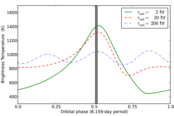
Our models show that for large radiative timescales, the temperatures at secondary eclipse are lower than 1150 K, regardless of $\omega_{\rm rot}$. For radiative times shorter than $\sim 10^{2}$ hr, the temperatures can be as high as 1400 K, similar to the 3.6-m measurement (Figure 9, top panel). However, these models still cannot explain the observed brightness-temperature discrepancy with wavelength.

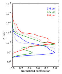
The study of eccentric hot-Jupiter atmospheric circulation by Kataria et al. (2012) hints at a resolution to this discrepancy. Their Figure 4 (top panel) shows that, as the planet passes through periapsis, the time that the peak temperature is reached varies as a function of pressure. This is typical of their simulations (T. Kataria 2009, private communication). If this differential response is significant in WASP-8b, it would introduce a discrepancy in the observations since the Spitzer bands sample different altitudes (see Figure 9 right panel).

Another possibility is to compare the radiative and advective timescales at the altitudes sampled by each band. Evaluating equation (1) of Fortney et al. (2008) using WASP-8b’s $P$–$T$ profile, indicates that $\tau$rad increases with depth between 0.1 and 1.0 bar, so there should be less longitudinal temperature contrast at depth. On the other hand, models of Kataria et al. (2012) show that wind speeds decrease with depth, and thus $\tau$adv also increases with depth. If the increase of $\tau$adv with depth is sharper than that of $\tau$rad, then one would expect less-homogenized temperatures at depth (but still above the photosphere). Hence, the rise in temperature (due to the increasing incident irradiation) near periapsis could be more pronounced at 3.6 m than at longer wavelengths, given the weighting functions of Figure 8.

7. Conclusions

Spitzer observed secondary eclipses of WASP-8b in the 3.6, 4.5, and 8.0 m IRAC wavebands. In our joint-fit model, we estimate eclipse depths of $0.113\%\pm 0.018\%$, $0.069\%\pm 0.007\%$, and $0.093\%\pm 0.023\%$ at 3.6, 4.5, and 8.0 m, respectively. These depths correspond to brightness temperatures of 1552, 1131, and 938 K, respectively. Although the 3.6-m eclipse depth is unexpectedly large, most of the ramp models had consistent depths (within 1$\sigma$), while those with inconsistent depths fit the data poorly.

Considering the $P$–$T$ profile of WASP-8b, KCl, ZnS, Li$2$, LiF, or Na$2$S clouds could form (see Figure 2(a) of Lodders & Fegley, 2006). In analogy to brown dwarfs, partial cloud coverage can cause photometric variability (Artigau et al., 2009); however, our three 4.5 m observations, spanning 1.5 years, have consistent eclipse depths, suggesting no temporal variation at secondary eclipse above a hemispheric-mean level of $\sim 35$ K (1$\sigma$). A moderate cloud layer at altitudes higher than those probed by Spitzer would produce a featureless planetary spectrum at wavelengths shorter than 2 m (Pont et al., 2008; Miller-Ricci Kempton et al., 2012) and would block some of the stellar flux, decreasing the temperatures at levels probed by Spitzer. Yet, the observed temperatures, which exceed the time-averaged equilibrium temperature, challenge this idea.

Given the high eccentricity, spin-orbit misalignment, and observed RV drift in the of WASP-8 system, Queloz et al. (2010) suggested the existence of an additional, unseen body in the system. Our orbital analysis is consistent with theirs. It also improves the orbital parameters and extends the baseline of sampled epochs. This constrains the long-term evolution of the orbit and aids the search for a second planet, for example through the study of timing variations (e.g., Agol et al., 2005).

The eclipse depths probe the dayside atmosphere of WASP-8b. Our results rule out the presence of a thermal inversion layer, as expected, given the irradiation level from the host star. A model with solar-abundance composition explains the 4.5 and 8.0 m planet-star flux contrast; however, including the high 3.6 m flux contrast requires models that output nearly 20% of the orbit-averaged incident irradiation, independent of the atmospheric composition. If the orbit were circular (and thus the irradiation steady-state), the high brightness temperatures would indicate a very low energy redistribution to the night side of the planet. For an eccentric planet, it at least indicates a short $\tau$rad (Figure 9).

By modeling the orbital thermal variations due to the eccentricity of the orbit, we determined that it is possible for WASP-8b to achieve temperatures as high as the 3.6 m brightness temperature. However, the differing brightness temperatures in the other two bands remain puzzling. Neither the radiative-transfer model (Section 5) nor the phase-variation model (Section 6) embraces all the physics of the problem. The radiative transfer code is a 1D, steady-state model representing typical dayside conditions. The phase-variation model describes emission as a blackbody on a single-layer grid; it does not consider absorption or emission features from the species in the atmosphere. Clouds (e.g., Cushing et al., 2008), atmospheric dynamics (e.g., Showman et al., 2009), and photochemistry (e.g., Moses et al., 2011) are not directly considered by these models.

What we can say for certain is that the assumptions of our simple models have been violated, which is not surprising for this eccentric planet. While it may be possible to construct consistent, realistic models, model uniqueness may be elusive until more and better data are available.

Relatively few exoplanets with equilibrium temperatures below 1500 K have been observed at secondary eclipse (Cowan & Agol, 2011b). The same is true for eccentric planets. The characterization of WASP-8b in this work thus addresses a particularly interesting, and challenging, region of the exoplanet phase space. Observation of other planets with similar equilibrium temperatures or eccentricities will help discover the physics that drive these unusual atmospheres.

References

- Agol et al. (2010) Agol, E. et al. 2010, ApJ, 721, 1861, ADS, 1007.4378
- Agol et al. (2005) Agol, E., Steffen, J., Sari, R., & Clarkson, W. 2005, MNRAS, 359, 567, ADS, astro-ph/0412032
- Anderson et al. (2011) Anderson, D. R. et al. 2011, MNRAS, 416, 2108, ADS, 1101.5620
- Artigau et al. (2009) Artigau, É., Bouchard, S., Doyon, R., & Lafrenière, D. 2009, ApJ, 701, 1534, ADS, 0906.3514
- Barman et al. (2005) Barman, T. S., Hauschildt, P. H., & Allard, F. 2005, ApJ, 632, 1132, ADS, arXiv:astro-ph/0507136
- Blecic et al. (2013) Blecic, J. et al. 2013, ApJ, submitted, (arXiv:1111.2363), ADS, 1111.2363
- Bodenheimer et al. (2001) Bodenheimer, P., Lin, D. N. C., & Mardling, R. A. 2001, ApJ, 548, 466, ADS
- Borysow (2002) Borysow, A. 2002, A&A, 390, 779, ADS
- Bouchy et al. (2005) Bouchy, F. et al. 2005, A&A, 431, 1105, ADS, arXiv:astro-ph/0410346
- Burrows et al. (2008) Burrows, A., Budaj, J., & Hubeny, I. 2008, ApJ, 678, 1436, ADS, 0709.4080
- Burrows et al. (2007) Burrows, A., Hubeny, I., Budaj, J., Knutson, H. A., & Charbonneau, D. 2007, ApJ, 668, L171, ADS, 0709.3980
- Burrows & Sharp (1999) Burrows, A., & Sharp, C. M. 1999, ApJ, 512, 843, ADS, arXiv:astro-ph/9807055
- Campo et al. (2011) Campo, C. J. et al. 2011, ApJ, 727, 125, ADS, 1003.2763
- Castelli & Kurucz (2004) Castelli, F., & Kurucz, R. L. 2004, arXiv:astro-ph/0405087, ADS, astro-ph/0405087
- Charbonneau et al. (2005) Charbonneau, D. et al. 2005, ApJ, 626, 523, ADS, arXiv:astro-ph/0503457
- Cowan & Agol (2011a) Cowan, N. B., & Agol, E. 2011a, ApJ, 726, 82, ADS, 1011.0428
- Cowan & Agol (2011b) —. 2011b, ApJ, 729, 54, ADS, 1001.0012
- Cowan et al. (2012) Cowan, N. B. et al. 2012, ApJ, 747, 82, ADS, 1112.0574
- Crossfield et al. (2012) Crossfield, I. J. M., Barman, T., Hansen, B. M. S., Tanaka, I., & Kodama, T. 2012, ApJ, 760, 140, ADS, 1210.4836
- Crossfield et al. (2010) Crossfield, I. J. M. et al. 2010, ApJ, 723, 1436, ADS, 1008.0393
- Cushing et al. (2008) Cushing, M. C. et al. 2008, ApJ, 678, 1372, ADS, arXiv:0711.0801
- Deming et al. (2007) Deming, D. et al. 2007, ApJ, 667, L199, ADS, 0707.2778
- Deming et al. (2011) —. 2011, ApJ, 726, 95, ADS, 1011.1019
- Eastman et al. (2010) Eastman, J., Siverd, R., & Gaudi, B. S. 2010, PASP, 122, 935, ADS, 1005.4415
- Fazio et al. (2004) Fazio, G. G. et al. 2004, ApJS, 154, 10, ADS
- Fortney et al. (2008) Fortney, J. J., Lodders, K., Marley, M. S., & Freedman, R. S. 2008, ApJ, 678, 1419, ADS, 0710.2558
- Freedman et al. (2008) Freedman, R. S., Marley, M. S., & Lodders, K. 2008, ApJS, 174, 504, ADS, 0706.2374
- Fressin et al. (2010) Fressin, F. et al. 2010, ApJ, 711, 374, ADS, arxiv:0909.5221
- Gelman & Rubin (1992) Gelman, A., & Rubin, D. B. 1992, Statistical Science, 7, 457
- Gillon et al. (2007) Gillon, M. et al. 2007, A&A, 471, L51, ADS, 0707.2261
- Goldreich & Soter (1966) Goldreich, P., & Soter, S. 1966, icarus, 5, 375, ADS
- Harrington et al. (2007) Harrington, J., Luszcz, S. H., Seager, S., Deming, D., & Richardson, L. J. 2007, Nature, 447, 691, ADS
- Hut (1981) Hut, P. 1981, A&A, 99, 126, ADS
- Ivanov & Papaloizou (2007) Ivanov, P. B., & Papaloizou, J. C. B. 2007, MNRAS, 376, 682, ADS, arXiv:astro-ph/0512150
- Kataria et al. (2012) Kataria, T. et al. 2012, ArXiv e-prints, ADS, 1208.3795
- Knutson et al. (2008) Knutson, H. A., Charbonneau, D., Allen, L. E., Burrows, A., & Megeath, S. T. 2008, ApJ, 673, 526, ADS, 0709.3984
- Knutson et al. (2009) Knutson, H. A. et al. 2009, ApJ, 703, 769, ADS, 0908.1977
- Knutson et al. (2010) Knutson, H. A., Howard, A. W., & Isaacson, H. 2010, ApJ, 720, 1569, ADS, arXiv:1004.2702
- Knutson et al. (2011) Knutson, H. A. et al. 2011, ApJ, 735, 27, ADS, 1104.2901
- Langton & Laughlin (2008) Langton, J., & Laughlin, G. 2008, ApJ, 674, 1106, ADS, 0711.2106
- Liddle (2007) Liddle, A. R. 2007, MNRAS, 377, L74, ADS, arXiv:astro-ph/0701113
- Lodders & Fegley (2006) Lodders, K., & Fegley, Jr., B. 2006, Chemistry of Low Mass Substellar Objects, ed. J. W. Mason, 1, ADS
- Machalek et al. (2008) Machalek, P. et al. 2008, ApJ, 684, 1427, ADS, arXiv:0805.2418
- Madhusudhan et al. (2011) Madhusudhan, N. et al. 2011, Nature, 469, 64, ADS, 1012.1603
- Madhusudhan & Seager (2009) Madhusudhan, N., & Seager, S. 2009, ApJ, 707, 24, ADS, 0910.1347
- Madhusudhan & Seager (2010) —. 2010, ApJ, 725, 261, ADS, arXiv:1010.4585
- Madhusudhan & Seager (2011) —. 2011, ApJ, 729, 41, ADS, 1004.5121
- Mandel & Agol (2002) Mandel, K., & Agol, E. 2002, ApJ, 580, L171, ADS, arXiv:astro-ph/0210099
- Miller-Ricci Kempton et al. (2012) Miller-Ricci Kempton, E., Zahnle, K., & Fortney, J. J. 2012, ApJ, 745, 3, ADS, 1104.5477
- Morales-Calderón et al. (2006) Morales-Calderón, M. et al. 2006, ApJ, 653, 1454, ADS, arXiv:astro-ph/0607537
- Moses et al. (2011) Moses, J. I. et al. 2011, ApJ, 737, 15, ADS, 1102.0063
- Nymeyer et al. (2011) Nymeyer, S. et al. 2011, ApJ, 742, 35, ADS, 1005.1017
- Peale (1999) Peale, S. J. 1999, ARA&A, 37, 533, ADS
- Pont et al. (2005) Pont, F. et al. 2005, A&A, 438, 1123, ADS, arXiv:astro-ph/0501615
- Pont et al. (2011) Pont, F., Husnoo, N., Mazeh, T., & Fabrycky, D. 2011, MNRAS, 414, 1278, ADS, 1103.2081
- Pont et al. (2008) Pont, F., Knutson, H., Gilliland, R. L., Moutou, C., & Charbonneau, D. 2008, MNRAS, 385, 109, ADS, 0712.1374
- Pont et al. (2006) Pont, F., Zucker, S., & Queloz, D. 2006, MNRAS, 373, 231, ADS, arXiv:astro-ph/0608597
- Queloz et al. (2010) Queloz, D. et al. 2010, A&A, 517, L1+, ADS, 1006.5089
- Ragozzine & Wolf (2009) Ragozzine, D., & Wolf, A. S. 2009, ApJ, 698, 1778, ADS, 0807.2856
- Seager & Hui (2002) Seager, S., & Hui, L. 2002, ApJ, 574, 1004, ADS, arXiv:astro-ph/0204225
- Showman et al. (2009) Showman, A. P. et al. 2009, ApJ, 699, 564, ADS, 0809.2089
- Southworth (2008) Southworth, J. 2008, MNRAS, 386, 1644, ADS, 0802.3764
- Spiegel et al. (2009) Spiegel, D. S., Silverio, K., & Burrows, A. 2009, ApJ, 699, 1487, ADS, 0902.3995
- Stevenson et al. (2012) Stevenson, K. B. et al. 2012, ApJ, 754, 136, ADS, 1108.2057
- Stevenson et al. (2010) Stevenson, K. B. et al. 2010, Nature, 464, 1161, ADS, arXiv:1010.4591
- Werner et al. (2004) Werner, M. W. et al. 2004, ApJS, 154, 1, ADS, astro-ph/0406223
- Winn et al. (2008) Winn, J. N., Henry, G. W., Torres, G., & Holman, M. J. 2008, ApJ, 675, 1531, ADS, 0711.1888
- Wu & Murray (2003) Wu, Y., & Murray, N. 2003, ApJ, 589, 605, ADS, arXiv:astro-ph/0303010
- Zahnle et al. (2009) Zahnle, K., Marley, M. S., Freedman, R. S., Lodders, K., & Fortney, J. J. 2009, ApJ, 701, L20, ADS, 0903.1663