Anisotropic charge screening and supercell size convergence of defect formation energies

Abstract

One of the main sources of error associated with the calculation of defect formation energies using plane-wave Density Functional Theory (DFT) is finite size error resulting from the use of relatively small simulation cells and periodic boundary conditions. Most widely-used methods for correcting this error, such as that of Makov and Payne, assume that the dielectric response of the material is isotropic and can be described using a scalar dielectric constant $\epsilon$. However, this is strictly only valid for cubic crystals, and cannot work in highly-anisotropic cases. Here we introduce a variation of the technique of extrapolation based on the Madelung potential, that allows the calculation of well converged dilute limit defect formation energies in non-cubic systems with highly anisotropic dielectric properties. As an example of the implementation of this technique we study a selection of defects in the ceramic oxide Li₂TiO₃ which is currently being considered as a lithium battery material and a breeder material for fusion reactors.

I Introduction

Point defects play an essential role in a number of important materials properties such the accommodation of nonstoichiomety and facilitation of diffusion through a crystal matrix. The difficulties associated with making direct observations on such small length scales mean it is desirable for first principles methods such as Density Functional Theory (DFT) to provide insight into the properties and behaviour of both intrinsic and extrinsic point defects.

In DFT, point defects are normally modelled using the supercell methodology, whereby vacancy, interstitial or substitutional defects are placed in a simulation supercell which is then tesselated though space using periodic boundary conditions (PBCs) to create an infinite crystal. Therefore, any defect included in the original supercell will also be tesselated and the interaction of these defect images can have a significant influence on the defect formation energy. This problem is particulary acute in the case of charged defects as the Coulomb interaction decays slowly as a function of the separation between point chargesNieminen (2009). A number of correction schemes have been devised to extract the formation energies in the desired dilute limit from simulations of relatively small supercells: these have been widely applied to systems such as silicon Taylor and Bruneval (2011); Corsetti and Mostofi (2011), NaClTaylor and Bruneval (2011); Schultz (2000), diamond Freysoldt et al. (2009, 2011), GaAsLany and Zunger (2008, 2009); Freysoldt et al. (2009, 2011), InP Castleton and Mirbt (2004) and Al₂O₃Hine et al. (2009, 2010). Inherent in all of these schemes is the assumption that the dielectric response of the material is isotropic and can be described by a single dielectric constant, $\epsilon$. Strictly, this only holds for cubic systems, but in many cases the degree of anisotropy is modest enough that the assumption of an isotropic dielectric response is adequate Hine et al. (2009); Lany and Zunger (2009); Malone and Cohen (2012). Intuitively, one might expect that this would not be the case for many of the more complex crystals that are currently being proposed for industrial applications, particularly those with layered structures.

One such system is lithium metatitanate, $\beta$-Li₂TiO₃, which is currently under consideration for use in lithium ion batteries Zhang et al. (2004) and as breeder material in fusion reactors Raffray et al. (2002). Li₂TiO₃ may be described as a distorted rocksalt structure (space group $C2/c$) with alternating Li, LiTi₂ and O planesLang (1954); Kataoka et al. (2009); Murphy et al. (2011) which are clearly visible in Fig. 1. Within the LiTi₂ layers the Ti atoms form a honeycomb structure with a Li ion at the centre of each hexagon. It is this layered structure that gives rise to the material’s interesting dielectric properties. Currently, not much is known about the properties of the defects in Li₂TiO₃. Vijayakumar et al. determined, using empirical potentials, the relative energies required to remove the different Li atoms and found that the formation energy of a Li vacancy defect in the pure Li layer is 0.30 eV greater than in the LiTi₂ layerVijayakumar et al. (2009). The linear “muffin-tin” orbitals method has been used to study H substitution onto Li sites where the hydrogen is observed to move from the lithium site and bond to an oxygen forming a hydroxideZainullina et al. (2003). One of the principle reasons for this shortage of theoretical results is the very same problem we try to address in this paper: namely that the anisotropy of the system means that it is hard to extract well-converged formation energies.

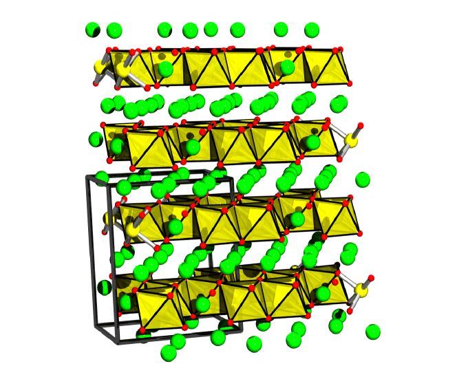
Figure 1: Crystal structure of $\beta-$Li₂TiO₃. Yellow, green and red spheres represent titanium, lithium and oxygen ions respectively. The black outline represents a single unit cell.

In this study we investigate the convergence of the formation energies of point defects in monoclinic $\beta-$Li₂TiO₃ as a function of supercell size. Specifically, we study the V${}_{\mathrm{Ti}}^{-4}$, Li${}_{\mathrm{Ti}}^{-3}$ and O${}_{i}^{-2}$ defects (modified Kröger-Vink notation). These defects represent a range of different defect types and also have high charge states and so are subject to the largest finite-size errors.

II Methodology

The DFT simulations presented here were performed using the plane-wave pseudo-potential code CASTEPClark et al. (2005). Exchange-correlation is described using the generalised gradient approximation of Perdew, Burke and Ernzerhof (GGA-PBE)Perdew et al. (1996). A $\Gamma$-centered Monkhorst-Pack Monkhorst and Pack (1976) scheme was used to sample the Brillouin zone with the separation of points maintained as close as possible to 0.05 Å^-1 along each axis.

The same pseudopotentials as in previous workMurphy et al. (2011) (ultrasoft pseudo-potentials (USPs), generated “on-the-fly” in CASTEP, and normconserving pseudopotentials (NCPPs) from the standard library in Materials Studio) were employed here. The planewave kinetic energies were truncated at 550 eV and 1700 eV for the USP and NCPPs respectively. The Fourier transform grid for the electron density is larger than that of the wavefunctions by a scaling factor of 2.0 and the corresponding scaling for the augmentation densities was set to 2.3 when USPs were in use. These values were determined by performing convergence tests of the energy from self consistent single point simulations. The lattice parameters determined using DFT are within 1$\%$ of the experimental as shown in Table 1. Additionally a comparison of all the atomic positions has been included in the Supplementary Materials.

Table 1: Table showing the lattice parameters and bandgaps calculated using the Ultrasoft and Norm-conserving pseudo-potentials compared to the available experimental data.

Property	Ultrasoft	Norm-conserving	Experimental
Volume /Å3	432.98	441.53	427.01Kataoka et al. (2009)
a /Å	5.09	5.12	5.06Kataoka et al. (2009)
b /Å	8.83	8.90	8.79Kataoka et al. (2009)
c /Å	9.80	9.85	9.75Kataoka et al. (2009)
$\beta$ /∘	100.19	100.24	100.21 Kataoka et al. (2009)
$E_{g}$ /eV	3.27	3.43	3.90Hosogi et al. (2008)

Supercells for the defect simulations were then constructed by creating $l\times{m}\times{n}$ repetitions of the relaxed unitcell in $a$, $b$ and $c$ respectively with the resulting supercells containing between 192 and 576 atoms. The lattice parameters and cell angles were fixed during minimization of the defect containing supercells so only atom positions were relaxed until the residual force on each atom was $<0.08$ eV A^-1 and the difference in energy between consecutive ionic relaxation steps was $<5\times 10^{-5}$ eV atom^-1.

The calculated band gap of Li₂TiO₃ was 3.27 eV for the USPs and 3.43 eV for the NCPPs compared to an experimental value of 3.9 eVHosogi et al. (2008) and values of 2.5-3.5 eV from previous first principles studies Zainullina et al. (2003); Shein et al. (2011); Wan et al. (2012). Underestimation of the bandgap is a common feature of LDA and GGA calculations: fortunately the lack of occupied states in the band gap for the fully charged defects investigated here ensures that the defect formation energies reported are not directly affected by this source of errorHine et al. (2009), although there are still effects due to the localization of states. The implementation of a hybrid functional, such as the HSE functionalHeyd et al. (2003) would most likely change the defect formation energies. However, it is important to note that whatever functional is used, formation energies are still subject to similar finite-size effects, as these are determined almost entirely by the Coulombic interaction of periodic images, with functional-dependent effects being limited to the polarizability and localisation of charges.

Following the formalism of Zhang and Northup Zhang and Northup (1991) the formation energy of a defect is given by:

$$E_{f}=E_{\textrm{defect}}^{T}-E_{\textrm{perf}}^{T}+\sum_{i}{n_{i}}\mu_{i}+qE_{F}$$ (1)

where $E_{\textrm{defect}}^{T}$ and $E_{\textrm{perf}}^{T}$ are the DFT total energies of a system with and without the defect, $n_{i}$ is the number of atoms added/removed, $\mu_{i}$ is the chemical potential of species $i$, $q$ is the charge on the defect and $E_{F}$ is the Fermi energy (defined here as the valence band maximum, VBM).

Representative chemical potential potentials ($\mu_{\mathrm{Li}}$, $\mu_{\mathrm{Ti}}$ and $\mu_{\mathrm{O}}$) were generated starting from the assumption that Li₂TiO₃ can be formed from Li₂O and TiO₂ via reaction 2 (this approach has been adopted for simplicity, though we note that this is not the traditional route for synthesis of Li₂TiO₃Sinha et al. (2010)),

$$\centering\mathrm{Li}_{2}\mathrm{O}_{\left(\mathrm{s}\right)}+\mathrm{TiO}_{2\left(\mathrm{s}\right)}\rightarrow\mathrm{Li}_{2}\mathrm{TiO}_{3\left(\mathrm{s}\right)}.\@add@centering$$ (2)

The sum of the chemical potentials of the constituent species must equal the total Gibbs free energy of the Li₂TiO₃, i.e.

$$\centering\mu_{\mathrm{TiO}_{2}}\left(p_{O_{2}},T\right)+\mu_{\mathrm{Li}_{2}\mathrm{O}}\left(p_{O_{2}},T\right)=\mu_{\mathrm{Li}_{2}\mathrm{TiO}_{{3}\left(s\right)}}\@add@centering$$ (3)

where, $\mu_{\mathrm{TiO}_{2}}\left(p_{\mathrm{O}_{2}},T\right)$ and $\mu_{\mathrm{Li}_{2}\mathrm{O}}\left(p_{\mathrm{O}_{2}},T\right)$ are the chemical potentials of Li₂O and TiO₂ within lithium metatitanate as a function of oxygen partial pressure and temperature and $\mu_{\mathrm{Li}_{2}\mathrm{TiO}_{{3}\left(s\right)}}$ is the chemical potential of solid $\mathrm{Li}_{2}\mathrm{TiO}_{3}$. For a solid $\mu\left(\mathrm{O}_{2}^{\circ},T^{\circ}\right)\approx\mu\left(0,0\right)$ therefore the temperature and pressure dependencies have been dropped. Two limiting cases are envisaged, one in which the titanate is formed with excess Li₂O, ie. $\mu_{\mathrm{Li}_{2}\mathrm{O}}\left(p_{\mathrm{O}_{2}},T\right)=\mu_{\mathrm{Li}_{2}\mathrm{O}_{\left(s\right)}}$ and $\mu_{\mathrm{TiO}_{2}}\left(p_{\mathrm{O}_{2}},T\right)=\mu_{\mathrm{Li}_{2}\mathrm{TiO}_{{3}\left(s\right)}}-\mu_{\mathrm{Li}_{2}\mathrm{O}_{\left(s\right)}}$ and similarly titania rich formation conditions where $\mu_{\mathrm{TiO}_{2}}\left(p_{\mathrm{O}_{2}},T\right)=\mu_{\mathrm{TiO}_{2\left(s\right)}}$. Here we assume Li₂O-rich conditions, therefore $\mu_{\frac{1}{2}\mathrm{O_{2}}}\left(p_{\mathrm{O}_{2}}^{\circ},T^{\circ}\right)$ can be determined from the formation energy of Li₂O under standard conditions (taken from a thermochemical databaseChase Jr. et al. (1986)) and the DFT total energies for Li₂O and lithium metal. $\mu_{\frac{1}{2}\mathrm{O_{2}}}\left(p_{\mathrm{O}_{2}},T\right)$ can then be determined following Finnis et al. Finnis et al. (2005), $\mu_{\mathrm{Li}}\left(p_{\mathrm{O}_{2}},T\right)=1/2\left(\mu_{\mathrm{Li}_{2}\mathrm{O}}^{DFT}-\mu_{\frac{1}{2}\mathrm{O_{2}}}\left(p_{\mathrm{O}_{2}},T\right)\right)$ and similarly$\mu_{\mathrm{Ti}}\left(p_{\mathrm{O}_{2}},T\right)=\mu_{\mathrm{TiO}_{2}}^{DFT}-2\mu_{\frac{1}{2}\mathrm{O_{2}}}\left(p_{\mathrm{O}_{2}},T\right)$. For the purposes of this work a temperature of 1000 K and oxygen partial pressure of 0.2 atm were selected.

In a periodic system the electrostatic energy is only finite if the total charge on the repeat cell is zero. Therefore, when modelling a charged defect in a simulation cell subject to PBCs, a uniform jellium of charge is imagined to exactly neutralize the net charge on the supercellDabo et al. (2008). The electrostatic energy of a periodically repeating finite system containing a point charge, $q$, and a neutralizing background jellium is the Madelung energy,

$$\centering E=-\frac{q^{2}v_{M}}{2\epsilon}\@add@centering$$ (4)

where $v_{M}$ is the Madelung potential (for cubic systems $v_{M}=\alpha/L$, where $\alpha=2.8373$ and $L$ is the supercell size length). This energy (scaled by $\epsilon$ to represent dielectric screening in the material) arises due to the use of PBCs and is therefore an artifact of the simulation technique and must be removed from the calculated defect formation energy resulting in the charge correction proposed by Leslie and GillanLeslie and Gillan (1985):

$$\centering E_{f}^{\infty}=E_{f}(L)+\frac{q^{2}v_{M}}{2\epsilon}.\@add@centering$$ (5)

In highly ionic materials, defect charge distributions can be described as point like, so this correction is adequate Komsa et al. (2012), however when the defect charge distribution is more diffuse the correction of Makov and PayneMakov and Payne (1995) is more appropriate. Castleton and co-workers proposed an extrapolation procedureCastleton and Mirbt (2003, 2004) for the study of defects in InP whereby the limit of a fit to a series of formation energies obtained from supercells of increasing size was used to determine the formation energy of the isolated defect. However, uniformly scaling all axes simultaneously rapidly increases the number of atoms in the supercell. Consequently it is only computationally feasible to sample the smallest multiplications resulting in too few points to allow a reliable fit to the data. Hine et al. thus suggested an improvement to this scheme based on simulation of supercells comprising different multiples of the primitive cell along different axesHine et al. (2009), with $v_{M}$ calculated separately for each cell. By plotting the defect formation energy as a function of $v_{M}$ and fitting a function of the form $E_{f}\left(v_{M}\right)=E_{f}^{\infty}+bv_{M}$, it is possible to determine the formation energy of the defect in the dilute limit from the intercept with the $y$-axis, and an effective permittivity can be extracted from the gradient as $b=-q^{2}/2\epsilon$.

The constant $v_{M}$ can be found using Ewald summation Ewald (1921):

$$v_{M}=\sum_{\mathbf{R}_{i}}^{i\not=0}\frac{\text{erfc}\left(\gamma\sqrt{|\mathbf{R}_{i}|}\right)}{|\mathbf{R}_{i}|}+\sum_{\mathbf{G}_{i}}^{i\not=0}\frac{4\pi}{V_{c}}\frac{\exp\left(-\mathbf{G}_{i}^{2}/4\gamma^{2}\right)}{\mathbf{G}_{i}^{2}}-\frac{2\gamma}{\sqrt{\pi}}-\frac{\pi}{V_{c}\gamma^{2}}.$$ (6)

where the sum extends over all vectors of the direct ($\mathbf{R}_{i}$) and reciprocal ($\mathbf{G}_{i}$) lattices, $\gamma$ is a suitably chosen convergence parameter and $V_{c}$ is the volume of the supercell. $v_{M}$ is normally positive and hence the Madelung energy is normally negative as it is dominated by the interactions of the point charge and the canceling background jellium which is on average closer than the periodic images. For long, thin supercells this is no longer the case as the electrostatics are now dominated by the interactions of neighbouring point charges and so $v_{M}$ is negative. This can, however, be viewed as an advantage since simulations can be performed on supercells where $v_{M}$ is both negative and positive and the results interpolated to $v_{M}=0$ rather than performing an extrapolation outside the range for which data is available.

Fig. 2 shows the formation energy of the V${}_{\mathrm{Ti}}^{-4}$ defect as a function of $v_{M}$ for a range of supercell shapes and sizes. The data display a wide variation and it is not possible to extract a single value for $E_{f}^{\infty}$. The origin of this variation may be deduced by examining subsets of the data. Shown in Fig. 2 are fits of the form $E_{f}\left(v_{M}\right)=E_{f}^{\infty}+bv_{M}$ to defect formation energies calculated in supercells created by extrapolating in the number of repeat units along the $b$- and $c$-axes independently, i.e. 2$\times{m}\times$1 (for $m$= 2,3 and 4) and 2$\times$1$\times{n}$ (for $n$ = 2,3 and 4). As the effective permittivity can be related to the gradient of such a fit it is apparent that there is a different level of charge screening present along these crystallographic axes. The effective dielectric constant along $b$ (28.3) is predicted to be more than double that along $c$ (13.4).

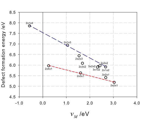
Figure 2: Formation energy of the V${}_{\mathrm{Ti}}^{-4}$ defect for a range of supercells with differing $v_{M}$. The wide variation in the points demonstrates that is not possible to fit a single straight line of the $E_{f}\left(v_{M}\right)=E_{f}^{\infty}+bv_{M}$ to the data.

To account for anisotropy in the screening, the dielectric constant in Eq. 5 must be replaced by a tensorRurali and Cartoixa (2009), denoted $\bar{\epsilon}$. For a monoclinic crystal such as Li₂TiO₃ the dielectric tensor has four non-zero components, as shown belowNye (1957):

$$\bar{\epsilon}=\left[\begin{array}[]{ccc}\epsilon_{11}&0&\epsilon_{13}\\ 0&\epsilon_{22}&0\\ \epsilon_{13}&0&\epsilon_{33}\end{array}\right]\,.$$ (7)

This tensor can then be incorporated into the Ewald summation to give a screened Madelung potential, $v_{M}^{\mathrm{scr}}$, in the general case Fischerauer (1997); Rurali and Cartoixa (2009):

$$v_{M}^{\mathrm{scr}}=\sum_{\mathbf{R}_{i}}^{i\not=0}\frac{1}{\sqrt{\det{\bar{\epsilon}}}}\frac{\text{erfc}\left(\gamma\sqrt{\mathbf{R}_{i}\cdot\bar{\epsilon}^{-1}{\cdot}\mathbf{R}_{i}}\right)}{\sqrt{\mathbf{R}_{i}{\cdot}\bar{\epsilon}^{-1}{\cdot}\mathbf{R}_{i}}}+\sum_{\mathbf{G}_{i}}^{i\not=0}\frac{4\pi}{V_{c}}\frac{\exp\left(-\mathbf{G}_{i}{\cdot}\bar{\epsilon}{\cdot}\mathbf{G}_{i}/4\gamma^{2}\right)}{\mathbf{G}_{i}{\cdot}\bar{\epsilon}{\cdot}\mathbf{G}_{i}}-\frac{2\gamma}{\sqrt{\pi\det{\bar{\epsilon}}}}-\frac{\pi}{V_{c}\gamma^{2}}.$$ (8)

Eq. 8 implies that it is necessary to determine the dielectric tensor for each defect cell, which while possible using Density Functional Perturbation Theory (DFPT)Refson et al. (2006), is computationally prohibitive. Here we investigate two possible methods that circumvent this problem.

In the region far from the defect the atomic positions (and consequently the dielectric properties) will remain largely unaffected by the presence of the defect, however, in the region immediately surrounding the defect the screening properties may be strongly perturbed. If the perturbed region is small relative to the simulation supercell then the dielectric properties of the whole cell may not undergo a substantial modification, As a first approximation, we therefore try applying the dielectric tensor for the perfect Li₂TiO₃ crystal to the all defective systems.

In our second approach a function $E_{f}(v_{M})=-(q^{2}/2)v_{M}+E_{f}^{\infty}$ is fitted to the defect formation energies determined for a number of different cell shapes and sizes. This fitting procedure is slightly unusual as it is the values in the $x$-axis that are modified by optimising the elements of $\bar{\epsilon}^{\mathrm{eff}}$. Optimised values of $E_{f}^{\infty}$ and the associated elements of $\bar{\epsilon}^{\mathrm{eff}}$ were obtained using a Nelder-Mead simplex algorithmNelder and Mead (1965).

III Results and discussion

The dielectric tensor for Li₂TiO₃ was calculated using DFPT and the norm-conserving pseudo-potentials. The results, presented in Table 2; show that there is indeed a significant level of anisotropy in the dielectric tensor. Examining only the principal (diagonal) elements of $\bar{\epsilon}^{\mathrm{DFPT}}$ we can see that the magnitude of $\epsilon_{33}^{\mathrm{eff}}$ is less than half that of $\epsilon_{11}^{\mathrm{eff}}$ and $\epsilon_{22}^{\mathrm{eff}}$. Taking the tensor average gives a value of 30.5, which can be compared to a value of 24 for a polycrystalline Li₂TiO₃ sampleBian and Dong (2010) (this value has been corrected to represent the theoretical density). The discrepancy between the experimental and theoretical dielectric properties may arise due to the inherent inability of DFT simulations to accurately reproduce experimentally observed band gaps. The values also deviate from those predicted by examining the subsets of the uncorrected data determined from Fig. 2.

Corrections such as that of Makov-PayneMakov and Payne (1995) are often performed with $\epsilon$ obtained from either DFPT or experiment. Fig. 3 shows defect formation energies for V${}_{\mathrm{Ti}}^{-4}$ for a selection of supercells as a function of $v_{M}^{\mathrm{scr}}$, employing $\bar{\epsilon}^{\mathrm{DFPT}}$. The data points show that while the level of scatter present in Fig. 2 has been reduced there is also a poor adherence to the linear relationship with gradient $-q^{2}/2$ expected from Eq. 5. This discrepancy arises as the use of the dielectric tensor calculated for the perfect cell, which thus neglects the atomic relaxations and the consequent modification of the local screening in the vicinity of the defect. The modification of the dielectric properties of the supercell is further supported by the change in the band gap of the material upon introduction of the defect. Plotted in Fig. 5 are the Densities of States (DOS) for the perfect Li₂TiO₃ as well as the defect containing supercells (all DOS are produced for the 2$\times 2\times 2$ supercell). Fig. 5 shows that the bandgaps in the defect containing supercells are reduced relative to the perfect supercell ($E_{g}(\mathrm{V}_{\mathrm{Ti}}^{-4})=2.46$ eV, $E_{g}(\mathrm{Li}_{\mathrm{Ti}}^{-3})=2.86$ eV and $E_{g}(\mathrm{O}_{i}^{-2})=2.12$ eV), which would suggest a perceptible change in the dielectric properties of the cell.

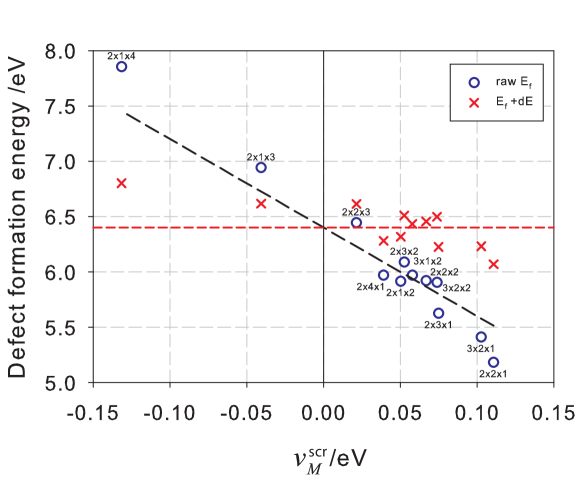
Figure 3: Formation energy of V${}_{\mathrm{Ti}}^{-4}$ as a function of $v_{M}^{\mathrm{scr}}$, where $\bar{\epsilon}^{\mathrm{DFPT}}$ has been used in the calculation of $v_{M}^{\mathrm{scr}}$. The black dashed line represents a fit of the form given in Eq 5 to the raw data and the red dashed line is fitted to the corrected data.

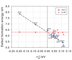
(a)

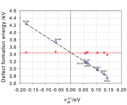
(b)

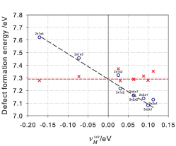
(c)

Figure 4: Defect formation energy as a function of $v_{M}^{\mathrm{scr}}$ for the (a) V${}_{\mathrm{Ti}}^{-4}$, (b) Li${}_{\mathrm{Ti}}^{-3}$ and (c) O${}_{i}^{-2}$ defects, where nonzero elements of $\bar{\epsilon}^{\mathrm{eff}}$ are fitted to the data. The wide variation in the data shown in Fig. 2 has disappeared, so one can interpolate to $v_{M}^{\mathrm{scr}}=0$ and extract defect formation energies in the dilute limit. Note that simulations in the largest 3$\times$2$\times$2, 2$\times$3$\times$2 and 2$\times$2$\times$3 supercells were only performed for the V${}_{\mathrm{Ti}}^{-4}$ defect.

In order to incorporate the change in the dielectric properties of the supercells induced by the defect, we instead fit the elements of $\bar{\epsilon}$ to give $\bar{\epsilon}^{\mathrm{eff}}$. $\bar{\epsilon}^{\mathrm{eff}}$ is then effectively an averaged picture of the dielectric tensors for the supercells included in the fit. Presented in Fig. 4 are plots of the formation energies as a function of $v_{M}^{\mathrm{scr}}$ after the fitting procedure has been performed for the V${}_{\mathrm{Ti}}^{-4}$, Li${}_{\mathrm{Ti}}^{-3}$ and O${}_{i}^{-2}$ defects. The three plots in Fig. 4 show that by fitting the elements of $\bar{\epsilon}$ it is possible to substantially improve the correlation between the data and the relationship given in Eq. 5, thus allowing a single linear function to be fitted to the data and a dilute limit defect formation energy to be extracted. Residual errors associated with the fitting process are around 0.1 eV and likely arise either from dipole-dipole or monopole-quadrupole interactions not accounted in Eq. 5, or from changes in atomic configurations for cells with one small value of $l$,$m$,$n$. The relatively small errors justify our treatment of the defect charge state as point-like. However in complex systems where the defect charge is less localised, or for defect clusters, this approximation may no longer hold.

Table 2: Effective permittivity tensor $\bar{\epsilon}^{\mathrm{eff}}$, and dilute limit defect formation energies $E_{f}^{\infty}$, for several defect species.

Species	$\epsilon_{11}^{\mathrm{eff}}$	$\epsilon_{22}^{\mathrm{eff}}$	$\epsilon_{33}^{\mathrm{eff}}$	$\epsilon_{13}^{\mathrm{eff}}$	$E_{f}^{\infty}$ /eV
Li2TiO3 (DFPT)	36.1	37.8	17.8	-5.0	-
$\mathrm{V}_{\mathrm{Ti}}^{-4}$	37.4	37.4	14.4	-1.0	6.3
$\mathrm{Li}_{\mathrm{Ti}}^{-3}$	34.9	35.0	13.9	-12.1	3.5
O${}_{i}^{-2}$	33.7	55.6	16.5	-8.9	7.3

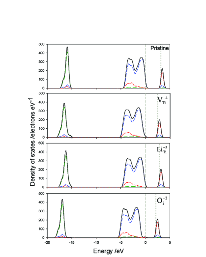
Figure 5: Densities of states for perfect Li₂TiO₃ and the V${}_{\mathrm{Ti}}^{-4}$, Li${}_{\mathrm{Ti}}^{-3}$ and O${}_{i}^{-2}$ defects. The long dashed green lines, intermediate dashed blue lines and short dashed red lines correspond to $s$-, $p$- and $d$-derived states respectively, with the sum plotted using the solid black line. The valence band maximum is indicated with a dashed grey vertical line and the conduction band minimum with a dotted grey vertical line.

The fitted elements of $\bar{\epsilon}^{\mathrm{eff}}$ and the resulting dilute-limit defect formation energies are presented in Table 2. In the case of the V${}_{\mathrm{Ti}}^{-4}$ and Li${}_{\mathrm{Ti}}^{-3}$ defects the degree of atomic relaxation is relatively small and the concomitant differences between $\bar{\epsilon}^{\mathrm{DFPT}}$ and $\bar{\epsilon}^{\mathrm{eff}}$ are also modest. The level of local distortion resulting from the introduction of an O${}_{i}^{-2}$ defect is much greater than for the other defects as depicted in Fig. 6. Furthermore the reduction in the bandgap is greatest for this defect which is also consistent with it displaying the most significant perturbation in its dielectric properties. It is this higher level of relaxation that leads to the increased difference between $\bar{\epsilon}^{\mathrm{DFPT}}$ and $\bar{\epsilon}^{\mathrm{eff}}$. At larger system sizes we would expect to recover values of $\bar{\epsilon}^{\mathrm{eff}}$ increasingly close to those of the perfect crystal, but the current results indicate that at the fairly small system sizes obtainable here, it is appropriate to fit to the observed results.

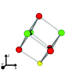
(a)

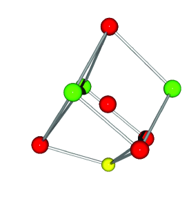
(b)

Figure 6: (a) Atomic arrangement surrounding an as yet unoccupied interstitial site in Li₂TiO₃ and (b) same atoms after introduction of an O${}_{i}^{-2}$ defect. Clearly visible in (a) is the distorted rocksalt structure of Li₂TiO₃ and the distortion arising arising due to the defect is illustrated in (b). It is this distortion that causes the significant change in $\bar{\epsilon}^{\mathrm{eff}}$ for this defect. All atom positions have been extracted from simulations in the 2$\times$2$\times$2 supercells.

IV Conclusions

In summary, we have proposed an extension of the Madelung extrapolation procedureHine et al. (2009) for the calculation of defect formation energies in the dilute limit. This is achieved by incorporating the effect of charge screening, via the dielectric tensor, into the calculation of the Madelung potential (via Eq. 8) and fitting the elements of the tensor and the desired dilute-limit formation energy to defect formation energies calculated in a range of supercells. We have applied the method to Li₂TiO₃, which has a monoclinic structure and a highly anisotropic dielectric tensor, and demonstrated its ability to determine defect formation energies converged to within around 0.1 eV even for such systems. In principle this method is applicable to systems of any shape and dielectric properties. Even in cubic supercells, local relaxation, such as that arising from defect clusters, may break the crystal symmetry such that the dielectric properties are anisotropic, necessitating a tensor representation of dielectric properties. We have also further highlighted the importance of incorporating the effect of lattice relaxation on the dielectric properties of the material when applying a finite-size correction method based on the Makov-PayneMakov and Payne (1995) approximation.

V Acknowledgments

Computational resources were provided by the Imperial College High Performance Computing Centre. Prof. Robin Grimes is thanked for useful discussions. NDMH acknowledges the support of EPSRC Grants EP/G05567X/1 and EP/J015059/1, and the Leverhulme Trust.

References

- Nieminen (2009) R. M. Nieminen, Modelling Simul. Mater. Sci. Eng., 17, 84001 (2009).
- Taylor and Bruneval (2011) S. E. Taylor and F. Bruneval, Phys. Rev. B, 84, 075155 (2011).
- Corsetti and Mostofi (2011) F. Corsetti and A. A. Mostofi, Phys. Rev. B, 84, 35209 (2011).
- Schultz (2000) P. A. Schultz, Phys. Rev. Lett., 84, 1942 (2000).
- Freysoldt et al. (2009) C. Freysoldt, J. Neugebauer, and C. G. Van de Walle, Phys. Rev. Lett., 102, 016402 (2009).
- Freysoldt et al. (2011) C. Freysoldt, J. Neugebauer, and C. G. Van de Walle, Phys. Status Solidi B, 248, 1067 (2011).
- Lany and Zunger (2008) S. Lany and A. Zunger, Phys. Rev. B, 78, 235104 (2008).
- Lany and Zunger (2009) S. Lany and A. Zunger, Modelling Simul. Mater. Sci. Eng., 17, 084002 (2009).
- Castleton and Mirbt (2004) C. W. M. Castleton and S. Mirbt, Phys. Rev. B, 70, 195202 (2004).
- Hine et al. (2009) N. D. M. Hine, K. Frensch, W. M. C. Foulkes, and M. W. Finnis, Phys. Rev. B, 79, 024112 (2009).
- Hine et al. (2010) N. D. M. Hine, P. D. Haynes, A. A. Mostofi, and M. C. Payne, J. Chem. Phys., 133, 114111 (2010).
- Malone and Cohen (2012) B. D. Malone and M. Cohen, J. Phys. Condens. Matter, 24, 055505 (2012).
- Zhang et al. (2004) L. Zhang, X. Wang, H. Noguchi, M. Yoshio, K. Takada, and T. Sasaki, Electrochim. Acta., 49, 3305 (2004).
- Raffray et al. (2002) A. R. Raffray, M. Akiba, V. Chuyanov, L. Giancarli, and S. Malang, J. Nucl. Mater., 307, 21 (2002).
- Lang (1954) A. Lang, Z. Anorg. Allg. Chem., 276, 77 (1954).
- Kataoka et al. (2009) K. Kataoka, Y. Takahashi, N. Kijima, H. Nagai, J. Akimoto, Y. Idemoto, and K. Ohshima, Mater. Res. Bull., 44, 168 (2009).
- Murphy et al. (2011) S. T. Murphy, P. Zeller, A. Chartier, and L. Van Brutzel, J. Phys. Chem. C, 115, 21874 (2011).
- Vijayakumar et al. (2009) M. Vijayakumar, S. Kerisit, Z. Yang, G. L. Graff, J. Liu, J. A. Sears, S. D. Burton, K. M. Rosso, and J. Hu, J. Phys. Chem. C, 113, 20108 (2009).
- Zainullina et al. (2003) V. M. Zainullina, V. P. Zhukov, T. A. Denisova, and L. G. Maksimova, J. Struct. Chem., 44, 180 (2003).
- Clark et al. (2005) S. J. Clark, M. D. Segall, C. J. Pickard, P. J. Hasnip, K. Refson, and M. C. Payne, Z. Kristallogr., 220, 1045 (2005).
- Perdew et al. (1996) J. P. Perdew, K. Burke, and M. Ernzerhof, Phys. Rev. Lett., 77(18), 3868 (1996).
- Monkhorst and Pack (1976) H. J. Monkhorst and J. D. Pack, Phys. Rev. B, 13, 5188 (1976).
- Hosogi et al. (2008) Y. Hosogi, H. Kato, and A. Kudo, J. Mater. Chem., 18, 647 (2008).
- Shein et al. (2011) I. R. Shein, T. A. Denisova, Y. V. Baklanova, and A. L. Ivanovskii, J. Struct. Chem., 52, 1043 (2011).
- Wan et al. (2012) Z. Wan, Y. Yu, H. F. Zhang, T. Gao, X. J. Chen, and C. J. Xiao, Eur. Phys. J. B, 85, 181 (2012).
- Heyd et al. (2003) J. Heyd, G. E. Scuseria, and M. Ernzerhof, J. Chem. Phys., 118, 8207 (2003).
- Zhang and Northup (1991) S. B. Zhang and J. E. Northup, Phys. Rev. Lett., 67, 2339 (1991).
- Sinha et al. (2010) A. Sinha, S. R. Nair, and P. K. Sinha, J. Nucl. Mater., 399, 162 (2010).
- Chase Jr. et al. (1986) M. W. Chase Jr., C. A. Davies, J. R. Downey, D. J. Frurip, R. A. McDonald, and A. N. Syverud, NIST JANAF thermochemical tables 1985 (NIST, 1986).
- Finnis et al. (2005) M. W. Finnis, A. Y. Lozovoi, and A. Alavi, Annu. Rev. Mater. Res., 35, 167 (2005).
- Dabo et al. (2008) I. Dabo, B. Kozinsky, N. E. Singh-Miller, and N. Marzari, Phys. Rev. B, 77, 115139 (2008).
- Leslie and Gillan (1985) M. Leslie and M. J. Gillan, J. Phys. C, 18, 973 (1985).
- Komsa et al. (2012) H.-P. Komsa, T. T. Rantala, and A. Pasquarello, Phys. Rev. B, 86, 45112 (2012).
- Makov and Payne (1995) G. Makov and M. C. Payne, Phys. Rev. B, 51, 4014 (1995).
- Castleton and Mirbt (2003) C. W. M. Castleton and S. Mirbt, Physica B, 340-342, 407 (2003).
- Ewald (1921) P. P. Ewald, Ann. Phys., 369, 253 (1921).
- Rurali and Cartoixa (2009) R. Rurali and X. Cartoixa, Nano Lett., 9, 975 (2009).
- Nye (1957) J. F. Nye, Physical Properties of Crystals (Oxford University Press, 1957) pp. 140–141.
- Fischerauer (1997) G. Fischerauer, IEEE Trans. Ultrason. Ferroelect. Freq. Contr., 44, 1179 (1997).
- Refson et al. (2006) K. Refson, S. J. Clark, and P. R. Tulip, Phys. Rev. B, 73, 155114 (2006).
- Nelder and Mead (1965) J. A. Nelder and R. Mead, Comput. J., 7, 308 (1965).
- Bian and Dong (2010) J. J. Bian and Y. F. Dong, J. Eur. Ceram. Soc., 30, 325 (2010).