Thermodynamics as a multistep relaxation process and the role of observables in different scales of quantities

Abstract

In the first part of the paper, we introduce the concept of observable quantities associated with a macroinstrument measuring the density and temperature and with a microinstrument determining the radius of a molecule and its free path length, and also the relationship between these observable quantities. The concept of the number of degrees of freedom, which relates the observable quantities listed above, is generalized to the case of low temperatures. An analogy between the creation and annihilation operators for pairs (dimers) and the creation and annihilation operators for particles (molecules) is carried out. A generalization of the concept of a Bose condensate is introduced for classical molecules as an analog of an ideal liquid (without attraction). The negative pressure in the liquid is treated as holes (of exciton type) in the density of the Bose condensate. The phase transition gas-liquid is calculated for an ideal gas (without attraction). A comparison with experimental data is carried out.

In the other part of the paper, we introduce the concept of new observable quantity, namely, of a pair (a dimer), as a result of attraction between the nearest neighbors. We treat in a new way the concepts of Boyle temperature $T_{B}$ (as the temperature above which the dimers disappear) and of the critical temperature $T_{c}$ (below which the trimers and clusters are formed). The equation for the Zeno line is interpreted as the relation describing the dependence of the temperature on the density at which the dimers disappear. We calculate the maximal density of the liquid and also the maximal density of the holes. The law of corresponding states is derived as a result of an observation by a macrodevice which cannot distinguish between molecules of distinct gases, and a comparison of theoretical and experimental data is carried out. In this paper, the observations in three scales, macro, micro, and nano, are studied.

1 Introduction

When introducing the concept of observable quantity in equilibrium thermodynamics, one must keep in mind the fact that the observation itself should be carried out in discrete intervals of time that are widely separated from one another. When standing on a purely mathematical point of view, one must agree that the processes of establishing an equilibrium require infinite time. However, in mathematics there are some concepts which are similar to the notion of “half-life” in physics. For example, one can introduce a time interval during which the difference between the current state and the state of equilibrium in the course of relaxation becomes $e$ times less.

In approximation theory and in the theory of numerical methods, especially after the well-known paper of Mandel’shtam and Leontovich [61], the following relaxation process was in use: at first, a reacting system is brought to some equilibrium. Then one rapidly changes one of the conditions (e.g., the temperature or the pressure) and traces the evolution of the system towards a new equilibrium (see, for example, the article “method – relaxation” in the Great Encyclopedia of Oil and Gas, http://www.ngpedia.ru [in Russian]).

Since the observation intervals should be “equal” to the relaxation time, they are large enough, and one can refer to the process as the multi-step relaxation process (MRP). Economic and historical processes, and also biological processes in a living organism, belong to phenomena of this kind, and therefore, from time to time, thermodynamic models of these processes arise. The formation of clusters, according to the scheme suggested below in Sec. 4.2, can serve as an example of a multi-step relaxation process.

The fact that time intervals of observation are discrete is the most important point to be taken into account when speaking about the instruments of observation.

The difference between readings of measuring macro- and microinstruments in thermodynamics is related to the following aspects.

1. A macroinstrument does not take into account the motions of nuclei, of electrons, and even of atoms within a molecule and regards any molecule as an individual particle. Mathematically, this corresponds to imposing rigid constraints on the elements forming the molecule. That is, we must modify those axioms of mechanics in which we consider all elementary particles and their behavior in the configuration space whose dimension is equal to the tripled number of elementary particles.

2. A macroinstrument measuring density counts the number of particles in a fragment of the volume; however, it cannot trace the movements of particles with different numbers during discrete finite time intervals. At each discrete time moment, this device counts the number of particles in the same fragment; however, it cannot notice what is the exact position of any particle indexed at the previous time moment and whether or not this particle really is within the chosen fragment. Mathematically, this means that the arithmetical law of rearrangement of summands holds. The sum does not depend on the way in which we have indexed the particles. In this sense, the laws of classical mechanics are even modified in a more substantial way.

Let us quote from the textbook [1] on quantum mechanics, where the authors define the basic property of classical mechanics: “In classical mechanics, identical particles (e.g., electrons) do not lose their ‘personality,’ despite the identity of their physical properties. Specifically, you can imagine that the particles forming a given physical system are ‘indexed’ at some time moment and then one can trace the motion of each of the particles along its own trajectory; then the particles can be identified at any time moment. …In quantum mechanics, it is fundamental that there is no way to trace each of the identical particles separately and thus to distinguish them. We can say that, in quantum mechanics, identical particles completely lose their individuality” (Russian p. 252).

A macroinstrument does not keep this basic property either. Mathematically, this means that, to take this property into account, we should impose some new constraints, which are already explicitly nonholonomic, on the mechanics of many particles and, which is especially important, we should take into account the permutability of particles in the definition of density, namely, any permutation of particles does not modify the density.

In thermodynamics, the gas molecule density is measured. Although the gas molecules differ from each other and the Boltzman approach to studying the molecules is consistent with the objective reality, the difference between the molecules does not play any role when the molecule density is determined. If the density is considered in a small fragment of the vessel, which contains approximately a million of particles, then it turns out that the density in this fragment coincides with the average density in the entire vessel up to a thousand of particles (up to 0.1 %) and is independent of the particle numeration.

It follows from these considerations that the entropy (in contrast to the Boltzmann–Shannon entropy) should take into account the permutability of the indices of the particles (cf. [2], Sec. 40).

Hence, for an ideal gas

$$\sum_{j}N_{j}=\sum_{j}G_{j}\bar{n}_{j}=N,\qquad\sum_{j}\varepsilon_{j}N_{j}=\sum_{j}\varepsilon_{j}G_{j}\bar{n}_{j}=E,$$ (1)

$$\frac{\partial}{\partial\bar{n}_{j}}(S+\alpha N+\beta E)=0,$$ (2)

where $\bar{n}_{j}$ stands for the average number of particles in each of the $G_{i}$ states of the $j$th group and $\alpha$ and $\beta$ are some constants (see [2], the footnote on p. 184, and also [4] and [5]), the entropy must be of the form

$$S=\sum_{j}\{(G_{j}+N_{j})\log(G_{j}+N_{j})-N_{j}\log N_{j}-G_{j}\log G_{j}\},$$ (3)

$$S=\sum_{j}G_{j}[(1+\bar{n}_{j})\log(1+\bar{n}_{j})-\bar{n}_{j}\log\bar{n}_{j}].$$ (4)

In other words, the entropy has exactly the same form as in the Bose–Einstein quantum case. This face is proved for balls and boxes in [2] in the footnote in Sec. 46; also see [4, 13].

We have noted above that a macroinstrument and its measurements force mathematicians to reorganize even the axioms of classical mechanics. However, mathematicians are forced to do so by entering the corresponding small parameters and passing to the related limits. A macroinstrument and its measurements still reduce the time spent to perform constructions of this kind. However, when one speaks of the axioms of thermodynamics, which is based on laws derived by great physicists who used ancient experiments conducted on Earth, it then turns out that the above considerations modify the classical concept of thermodynamics completely. Meanwhile, microinstruments also play a role in classical thermodynamics; they enable one to calculate the dimension related to the number of atoms in the molecule.

In the mathematical literature, as a rule, the number of degrees of freedom coincides with the number of independent generalized coordinates. However, there notions are distinct in the standard thermodynamics, because the volume is three-dimensional, which is established by the macrodevice, whereas the number of degrees of freedom is related to the number of atoms in a molecule and is measured by the microdevice.

Let us explain the following experimental fact. In some cases, the number of degrees of freedom for diatomic and polyatomic molecules is an integer. In our opinion, this happens because the intramolecular communications (the distances between the atoms of the molecule) are very hard, and, when the temperature increases, no new degrees of freedom arise. Generally speaking, the number of degrees of freedom fundamentally depends on the energy of the molecules, and the energy of different molecules of the same gas is different, and, apparently, to the average energy (the temperature) there must correspond the average number of degrees of freedom, which is hence must be noninteger. However, on one hand, tight connections enable one to excite almost all molecules for a sufficiently high (room) temperature and, on the other hand, to give the molecules no possibility to excite new degrees of freedom (e.g., the vibrational ones). If the connections are not so rigid, then the number of degrees of freedom depends on temperature, and hence on energy, and is not an integer in general. This is clear from the comparison of the values of the heat capacity $C_{V}$ with the experiment: for hydrogen sulfide with three atoms, the theory gives 5.96, and the experiment 6.08, for carbon dioxide, the experiment gives a greater value $C_{V}=6.75$ ($T=15C$, $P=1atm$), and, for carbon disulfide, the vale is almost two times larger, namely, 9.77. In the case of diatomic molecules, say, for nitrogen, the theory gives 4.967 and the experiment shows 4.93; for the chlorine, the value is almost 20% higher, namely, 5.93, etc.

It turns out that the number of degrees of freedom coincides with the dimension of the generalized Bose gas which is regarded as a distribution of a classical gas.

Landau and Lifshitz notice this fact for the three-dimensional Bose gas. They write that these equations ($PV^{5/3}=\text{const}$) coincide with the equations of the adiabatic line for an ordinary monatomic gas. “However, we stress,” the authors write further, “that the exponents in the formulas $VT^{3/2}=\text{const}$ and $PV^{5/3}=\text{const}$ are not related now to the ratio of specific heat capacities (since the relations $c_{p}/c_{v}=5/3$ and $c_{p}-c_{v}=1$ fail to hold)” [2], p. 187.

One can show in a quite similar way that, for the five-dimensional and six-dimensional Bose gas, the “Poisson adiabatic line” coincides with the Poisson adiabat for the two-atomic and three-atomic molecule (see [2], Sec. 47, Diatomic gas with molecules of different atoms. Rotation of molecules). With regard to the above stipulation, as $\mu\to-\infty$, we obtain precisely both the condition $c_{p}-c_{v}=1$ and the ratio $c_{p}/c_{v}$ coinciding with relations well known in the old thermodynamics.

Remark 1.

The three-dimensional case of the Bose–Einstein-type distribution can be represented as

$$N_{j}=\sum_{i+k+m=j}N_{i,k,m},$$

$$M=\sum_{i,k,m}(i+k+m)N_{i,k,m}=\sum_{j}\sum_{i+k+m=j}(i+k+m)N_{i,k,m}=$$

$$\sum_{j}\sum_{i+k+m=j}jN_{i,k,m}=\sum_{j}j\sum_{i+k+m=j}N_{i,k,m}=\sum_{j}jN_{j}.$$

The Bose–Einstein “average” values $\bar{n}_{i,k,m}$ of the occupation numbers $N_{i,k,m}$ depend only on the energy, i.e., on the sum $i+k+m$, and

$$\bar{n}_{i,k,m}=\frac{1}{e^{\beta(i+k+m-\mu)}-1},$$

so that

$$\bar{n}_{j}=\sum_{i+k+m=j}\bar{n}_{i,k,m}=\frac{q_{j}}{e^{\beta(i+k+m-\mu)}-1},\qquad q_{j}=\frac{(j+2)!}{j!3!}.$$

The transition to integer dimensions is similar; the fractional dimensions are obtained by passing from factorials to $\Gamma$-functions. A more rigorous approach in described in [13, 64, 65].

2 A new ideal gas and a new ideal liquid
as observable quantities

2.1 The number of degrees of freedom for $T\leq T_{c}$ and $P\leq P_{c}$

Let us now proceed with finding the number of degrees of freedom for for a low temperature that does not exceed the critical one: $T\leq T_{c}$.

The Maxwell–Boltzmann equation for the ideal gas is of the form

$$PV=NT,$$ (5)

where $P$ stands for the pressure, $V$ for the volume, $N$ for the number of particles, and $T$ for the temperature.

Denote by $Z$ the dimensionless quantity $Z=\frac{PV}{NT},$ which is called the compressibility factor. Equation 5 can be represented in the form $Z=1.$ Let us express the Bose–Einstein-type distribution for the fractional dimension $D$ using polylogarithms.

Represent the thermodynamic potential of the Bose gas of the fractional dimension $D=2(1+\gamma)$ in the form

$$\Omega(\mu,T)=(Cm)^{1+\gamma}V\frac{T^{2+\gamma}}{\Gamma(2+\gamma)}\int_{0}^{\infty}\frac{t^{1+\gamma}\,dt}{(e^{t}/a)-1}=-T^{2+\gamma}(Cm)^{1+\gamma}V\operatorname{Li}_{2+\gamma}(a),$$ (6)

where $T$ stands for the temperature, $m$ for the mass, $C$ is a constant, $a=\exp(\mu/T)$ is the activity, $\mu$ is the chemical potential, and $\Gamma$ stands for the Euler gamma function .

The function $\operatorname{Li}_{s}(a)$ introduced in 6 is referred to as a polylogarithm and is defined by the rule

$$\operatorname{Li}_{s}(x)=\frac{1}{\Gamma(s)}\int_{0}^{\infty}\frac{t^{s-1}}{(e^{t}/x)-1},\qquad\operatorname{Li}_{s}(1)=\zeta(s),$$ (7)

where $\zeta(s)$ stands for the Riemann zeta function.

To pass to the dimensionless units, we introduce the temperature $T_{r}$ in such a way that $T=T_{r}T_{c}$.

The expressions for the dimensionless pressure $P_{r}=P/P_{c}$ and for the number of particles $N$ that correspond to the thermodynamic potential 6 are of the form

$$P_{r}=\frac{T_{r}^{2+\gamma}\operatorname{Li}_{2+\gamma}(a)}{\zeta(2+\gamma)},$$ (8)

$$N=VT_{r}^{1+\gamma}\operatorname{Li}_{1+\gamma}(a).$$ (9)

We have (for the definition of $\gamma_{c}$, see below)

$$\Omega^{\prime}=-T_{r}^{2+\gamma}(Cm)^{\gamma_{c}-\gamma}V\operatorname{Li}_{2+\gamma}(a).$$ (10)

The following formula can thus be obtained for the compressibility factor $Z$:

$$Z=\frac{\operatorname{Li}_{2+\gamma}(a)}{\operatorname{Li}_{1+\gamma}(a)}.$$ (11)

In particular, for $a=1$ (i.e., for $\mu=0$), we have

$$Z=\frac{\zeta(\gamma+2)}{\zeta(\gamma+1)}.$$ (12)

As is well known, in the Bose–Einstein theory, the value $\mu=0$ corresponds to the so-called degeneration of the Bose gas.

For a classical gas satisfying the same relations, the degeneration coincides with the critical point $T=T_{c}$, $P=P_{c}$, and $Z=Z_{c}$. Consequently, one can write $\gamma=\gamma_{c}$ for $Z=Z_{c}$ in 12, namely,

$$Z_{c}=\frac{\zeta(\gamma_{c}+2)}{\zeta(\gamma_{c}+1)},$$ (13)

and to every pure classical gas there corresponds its own value of $\gamma_{c}$.

The entropy in the dimension $D=2\gamma+2$ can be evaluated in the standard way. The great thermodynamical potential is considered,

$$\Omega=-PV=-\frac{VT}{\Lambda^{2(1+\gamma)}}\cdot\frac{1}{\Gamma(2+\gamma)}\int_{0}^{\infty}\frac{t^{1+\gamma}\,dt}{(e^{t}/a)-1}=\frac{-VT^{2+\gamma}}{{\Lambda^{\prime}}^{2(1+\gamma)}}\operatorname{Li}_{2+\gamma}(a),$$

where $\Lambda^{\prime}=\text{const}/(2\pi m)^{1/2}$, the dimension $D$ is equal to $2\gamma+2$, $T$ stands for the temperature, and $a=e^{\mu/T}$ for the activity.

The number of particles is

$$N=-\frac{\partial\Omega}{\partial\mu}=\frac{VT^{1+\gamma}}{{\Lambda^{\prime}}^{2(1+\gamma)}}\operatorname{Li}_{1+\gamma}(a).$$

The compressibility factor is

$$Z=\frac{PV}{NT}=\frac{\operatorname{Li}_{2+\gamma}(a)}{\operatorname{Li}_{1+\gamma}(a)}.$$

Let us evaluate the entropy,

$$S=-\left(\frac{\partial\Omega}{\partial T}\right)_{V,\mu} =(2+\gamma)\frac{VT^{1+\gamma}}{{\Lambda^{\prime}}^{2(1+\gamma)}}\operatorname{Li}_{2+\gamma}(a)-\frac{VT^{1+\gamma}}{{\Lambda^{\prime}}^{2(1+\gamma)}}\operatorname{Li}_{1+\gamma}(a)\frac{\mu}{T}$$

$$=\frac{VT^{1+\gamma}}{{\Lambda^{\prime}}^{2(1+\gamma)}}\left[(2+\gamma)\operatorname{Li}_{1+\gamma}(a)-\operatorname{Li}_{1+\gamma}(a)\frac{\mu}{T}\right].$$

For $\mu=0$, $T_{r}=T/T_{c}$, and $P_{r}=P/P_{c}$, the specific entropy is equal to

$$\frac{S}{V}\big{|}_{\mu=0,T_{r}=1}=(2+\gamma)\zeta(2+\gamma).$$ (14)

E. M. Apfel’baum [Apfelbaum] and V. S. Vorob’ev [3] compared the Bose distributions of fractional dimension $D=2\gamma_{c}+2$ in the $(P,V)$ diagram with the experimental critical isotherms for various gases. We present these graphs in Figs. 1–5. In Fig. 5A, the graphs for the nitrogen and oxygen are shown, which have been constructed by Professor V. S. Vorob’ev.

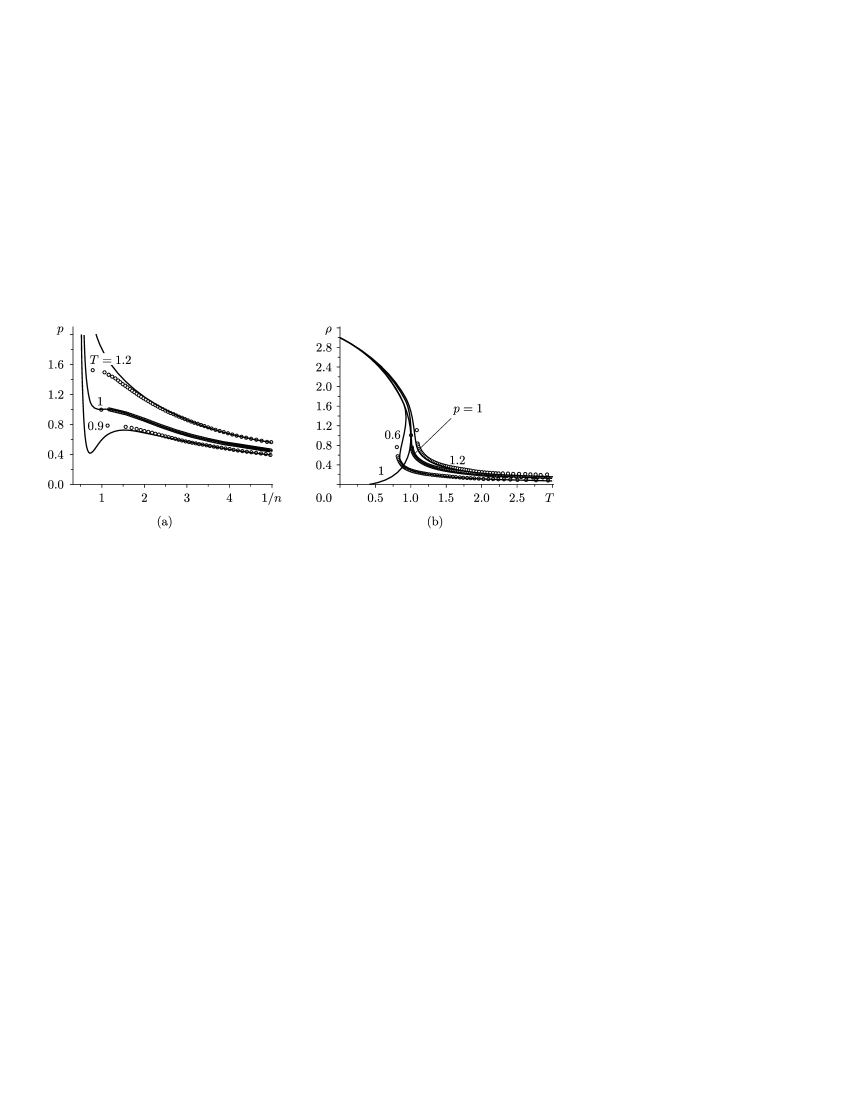
Figure 1: (a) Isotherms of pressure for the van der Waals equation are shown by solid lines. The lines formed by circles are constructed from computations for $\gamma=0.312$ (i.e., for the ideal “Bose gas”), $Z_{\mathrm{cr}}=3/8$, $p=P/P_{\mathrm{c}}$, and $n=N/N_{\mathrm{c}}$.
(b) Isobars of density for the van der Waals equation are shown by solid lines. Line 1 is the binodal. The circles correspond to isobars of the “Bose gas” for $\gamma=0.312$.

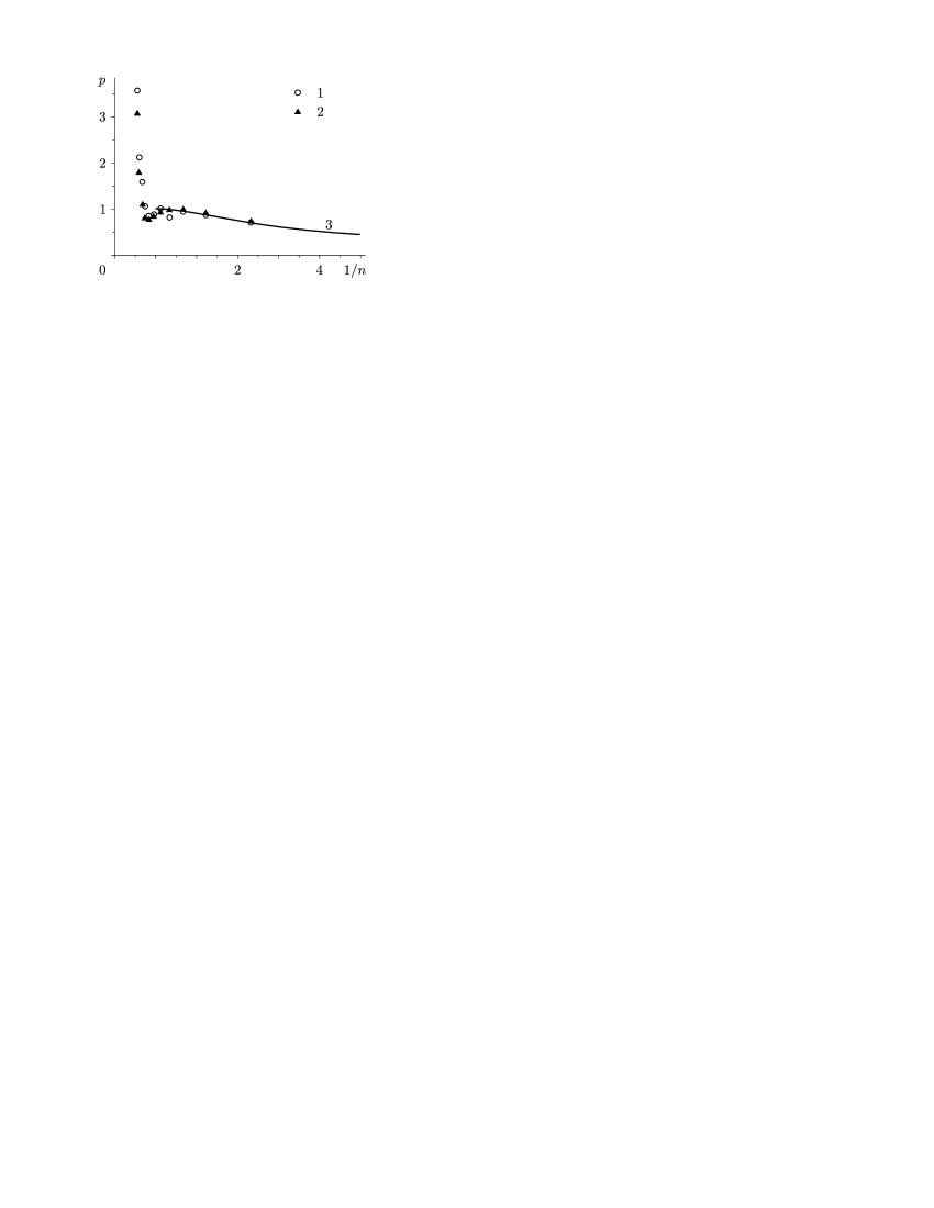
Figure 2: Critical isotherms for the Lennard–Jones system. Symbols 1 and 2 correspond to numerical calculations. Line 3 corresponds to the ideal Bose gas for $\gamma=0.24$.

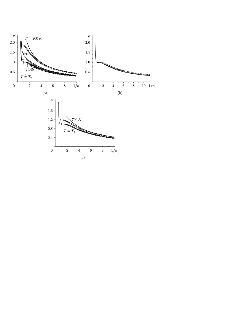
Figure 3: (a) Isotherms for argon. The solid lines correspond to experimental data. The line formed by circles is constructed in accordance with the isotherm of the ideal “Bose gas”; $Z_{\mathrm{cr}}=\frac{\zeta(\gamma+2)}{\zeta(\gamma+1)}=0.29$, $p=P/P_{\mathrm{c}}$, and $n=N/N_{\mathrm{c}}$.
(b) The same for water, $Z_{\mathrm{cr}}=0.23$.
(c) The same for copper, $Z_{\mathrm{cr}}=0.39$.

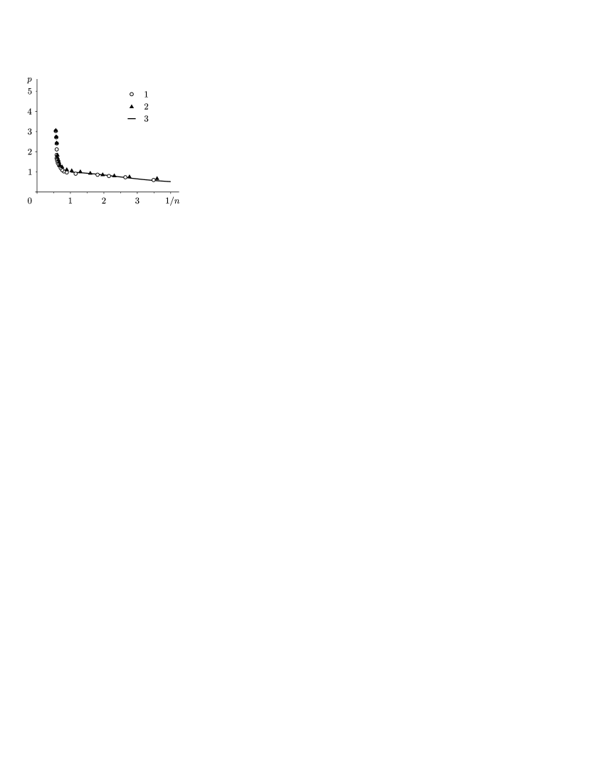
Figure 4: Isotherms for water. Symbols 1 and 2 correspond to experimental data, and line 3 corresponds to the computation for the Bose gas.

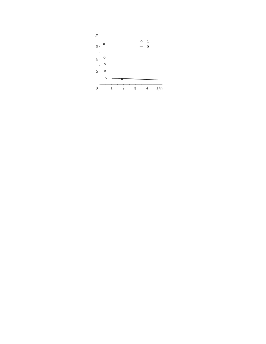
Figure 5: Critical isotherms for mercury. Symbols 1 and 2 correspond to experimental data, and line 3 corresponds to the computation for the Bose gas.

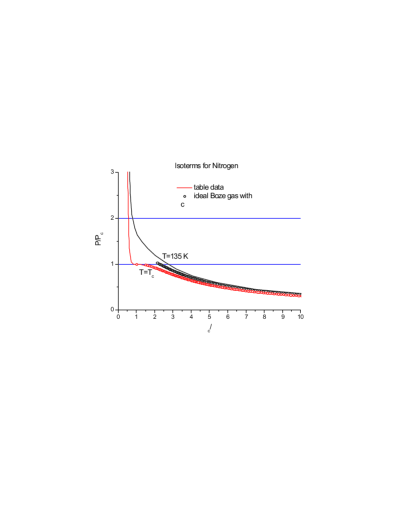
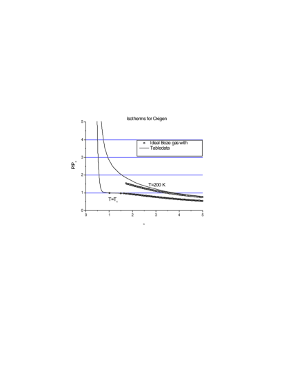
Figure 5A: 1. Isotherms for nitrogen. 2. Isotherms for oxygen.

2.2 Bose condensate as an observable quantity
in classical thermodynamics. Relativity principle for MRP

We shall show that the Bose condensate in classical thermodynamics is the condensate of gas (vapor) into liquid (in contrast to the statement presented in the manual [2] in the footnote on p. 199).

Example 1. Consider the example given by a famous theorem in number theory, namely, the solution of an ancient problem, which has the Latin title “partitio numerorum.” This task involves an integer $M$ which is decomposed into $N$ terms, for example, if $M=5$ and $N=2$, then $5=1+4=2+3,$ which gives two solutions to the problem, $\mathcal{M}=2$.

If $M=10^{23}$ and $N=1$, then the decomposition has only one version, and $\mathcal{M}=1$. If $M=10^{23}$ and $N=10^{23}$, then there is also only one version of decomposition, namely, the sum of ones, i.e., $\mathcal{M}=1$.

Obviously, there is a number $N_{c}$ for a fixed $M$ such that the number of versions of the decomposition, $\mathcal{M}$, is maximal possible (this number is not unique in general). The number $\log_{2}\mathcal{M}$ is referred to as the Hartley entropy. At the point at which $\mathcal{M}$ reaches its maximum, there is a maximum entropy.

Let a partition $M=a_{1}+\dotsb+a_{N}$ of $M$ into $N$ summands be given. Denote by $N_{j}$ the number of summands on the right-hand side that are precisely equal to $j$.

Then the total number of summands is $\sum_{j}N_{j}$, and this number is equal to $N$, since we know that the total number of summands is $N$. Further, the sum of the parts equal to $j$ is $jN_{j}$, since there are $N_{j}$ summands, and then the sum of all summands can be obtained by summing these expressions over all possible $j$, i.e., $\sum_{j}jN_{j}$, and this sum is equal to $M$. Namely,

$$\sum_{i=1}^{\infty}N_{i}=N,\qquad\sum_{i=1}^{\infty}iN_{i}=M.$$ (15)

The very nonuniqueness of the above maximum and an uncertainty concerning the number of the maxima enabled Erdős to obtain results with accuracy up to $o(\sqrt{M})$ only.

Thus, the Erdős theorem holds for the system of two Diophantine equations

$$\sum_{i=1}^{\infty}N_{i}=N,\qquad\sum_{i=1}^{\infty}iN_{i}=M.$$ (16)

The maximum number of solutions of the system is achieved provided that the following relation holds:

$$N_{c}=\beta^{-1}M_{c}^{1/2}\log\,M_{c}+\alpha M_{c}^{1/2}+o(M_{c}^{1/2}),\qquad\beta=\pi\sqrt{2/3},$$ (17)

and the coefficient $\alpha$ is defined by the formula $\beta/2=e^{-\alpha\beta/2}$.

If one increases the number $N$ in problem 16 and keeps the number $M$ constant, then the number of solutions decreases. If the sums in 16 are counted from zero rather than from one, i.e.,

$$\sum_{i=0}^{\infty}iN_{i}=(M-N),\qquad\sum_{i=0}^{\infty}{N_{i}}=N,$$ (18)

then the number of solutions does not decrease and remains constant.

Let us explain this fact. The Erdős–Lehner problem [6] is to decompose a number $M_{c}$ into $N\leq N_{c}$ summands.

The decomposition of the number 5 into two summands has two versions. If we include also 0, then we obtain three versions, 5+0 = 3+2 = 4+1. Thus, the inclusion of zero gives the opportunity to say that we decompose the number into $k\leq n$ summands. Indeed, the expansion of the number 5 into 3 summands includes all previous versions: 5 +0 +0, 3 +2 +0. and 4+1 +0 and adds new options that do not contain zero.

Here the maximum does not change much [6]; however, the number of options cannot decrease, because the zeros enable the maximum to remain constant, and the entropy never decreases; after reaching the maximum, it becomes constant. This very remarkable property of entropy enables us to construct a general unbounded probability theory [7]. In physics, the effect is identical to the so-called phenomenon of Bose condensate.

Let us pose the following question: what is the difference between arithmetic, together with the problem of “partitio numerorum,” and the Boltzmann–Shannon statistics? If we assume that $4+1$ and $1+4$ are two different versions, then we obtain the Boltzmann–Shannon statistics. The number of versions of decomposition, $\mathcal{M}$, is growing rapidly. Thus, the “noncommutativity” of the addition gives additionally a huge number of versions of decomposition, and the Hartley entropy (which is equal to the logarithm of the number of versions) coincides with the Boltzmann–Shannon entropy.

Therefore, we have proved that, if we add zero to the family of possible summands and decompose a number $M$ into $N$ summands, then this is equivalent to solving equations 18, i.e., to imposing relations for the number of particles and for energy. Here the number of zeros increases drastically; if $M=5$, then, for $N>3$, the number of zeros is 22. However, the number of ones is also large, although it is twice smaller than the number of zeros.

It is very visible to consider the Bose condensate as the number of zeros; however, this is inaccurate. The Bose condensate occurs in a neighborhood of a point at which the energy vanishes rather than at the point itself. Nevertheless, if one writes $\rho_{0}\delta(\mathbf{k})$ (where $\rho_{0}$ stands for the density and the vector $\mathbf{k}$ is the momentum) for the Bose condensate at rest, then this notation is true, because the density is the limit

$$\rho_{0}=\lim_{N\to\infty,V\to\infty}\frac{Nm}{V},$$

where $N$ stands for the number of particles, $V$ for the volume, and $m$ for the mass of the particle. This means that, as $N\to\infty$, the bell-shaped function near the zero energy is converted to the $\delta$ function.

By an ideal (or perfect) liquid we mean a liquid without attraction and without any surface tension. This is a liquid which can exist for a positive pressure only together with a saturated steam.

In this case, the perfect liquid is the result of an optical illusion, and this “perfect liquid” is the same ideal gas in the condensate, with another density. It can be described, as in the case of a consideration of a Bose condensate, in the form $\rho_{0}\delta(\mathbf{k})$, where $\rho_{0}$ stands for the density of the condensate. It cannot exist without a volume trap, which is similar to the case in which a container with gas has a hole, and there is a vacuum outside the vessel, in which case this liquid, which looks as if it is boiled, is going away together with the gas. The mean speed of the particles inside the liquid is the same as the mean speed of the gas particles. This corresponds to the condition that the temperature in the system “liquid–saturated steam” is the same in the liquid and in the gas. The liquid in a closed vessel is a fluctuation standing at a fixed place ($\delta(\mathbf{k})$), or, speaking in a simpler way, this liquid is a “resting” Bose condensate (cf. [8], p.204).

Small crystals that occur in a supersaturated solution coincide with the Bose condensate only if they are not composed of mutually connected particles, and, moreover, if the particles are continuously exchanged with the particles in the solution; moreover, the small crystals, as solids, are an optical illusion, namely, we simply do not see that the particles of crystals are permanently transposed with particles of the solution. In other words, this is by no means a crystal, this is a fluctuation; however, this fluctuation is relatively immobile.

Thus, the Bose condensate for classical particles represents some “special density fluctuations;” only this, and nothing more.

A. I. Anselm constructed his theory starting from the Eyring formula for free energy. The liquid structure model accepted by Eyring is in fact closer to the strongly compresses gas model [66, 67].

One can talk about the density in a “special cluster fluctuation” of a part of our vessel with gas. If we speak of the density in this cluster only, this means that (as in the example of a small volume with one million of particles) one cannot speak of the number of particles that are placed in the cluster as if they are frozen and do not move. This is only an appearance, and all of the particles or a part of them can be replaced in a minute by another ones, and the indexing inside the “fluctuation” cluster can change every minute. At the next time step, this can be the same picture but probably with different particles involved.

We speak about some fragment of the volume. In fact, the particles that are more concentrated can be spread out over the entire vessel. However, if there is at least a little gravity of the Earth, then the fluctuations with more concentrated particles accumulate near the bottom. If we consider a vessel with gas in the form of a perfectly reflecting sphere (see [9]–[12]), then, due to the repulsive force occurring at the border, fluctuations of this kind are located near the center of the ball.

From the standpoint of our observation, in discrete time intervals at far distances from each other, the denser fragment of the volume, i.e., the Bose condensate, is at rest and hence corresponds to a small momentum in the Bose–Einstein-type distribution. Mathematically, the MRP model corresponds to this phenomenon. This property will be called the relativity principle for MRP.

Let us repeat once again that the only fact which can be guaranteed by the generalized theory of Bose condensate is that there will be a higher density of particles at the bottom.

Example 2. Let a gas be contained in a closed vessel at a room temperature, and let the gas be almost satisfying the Clausius relation

$$P=\rho T.$$ (19)

We cool the vessel down to a temperature $T=0$. At some temperature $T\geq T_{0}$, a liquid is formed. The temperature $T_{0}$ is referred to as the dew point. According to the standard conception, the fluctuations above the temperature of the dew point are of the order of $\sqrt{N}$. After the formation of liquid, the gas, which is called a saturated steam in the physical literature, also satisfies relation 19. It is quite rarefied. According to the van der Waals model, there are no singularities at the dew point under the gas-liquid passage (on the so-called binodal). According to experimental data, there are no large fluctuations either in the usual sense at the dew point.

Finally, the most important thing. The experiment shows that, at $T=T_{0}$, the gas is rarefied, and it remains an ideal gas in the sense of relation 19, i.e., in the Boltzmann-Maxwell sense.

There is, however, a fluctuation of the type of a stationary Bose–Einstein condensate. in this fluctuation, the molecules by themselves placed inside this fluctuational fragment can possibly move with the same velocities as those of the gas molecules and, if it were possible to enumerate them, then the numbers will be changed very quickly. If shall refer to this fluctuation (of the form of the Bose-Einstein condensation) as liquid, then actual molecules of the liquid move in it with the same speeds as the gas molecules (of the “saturated vapor”).

To represent this picture in a more visible way, imagine a bunting which winds from one roller to the other. Between the rollers, under the material, a strong wind blows from a hose. We see a “ hump” is formed between the rollers; however, it can be assumed that we do not see that the bunting moves.

Nevertheless, as the density of the Bose condensate increases, our macroinstrument can fix the bound of the density and show us that there is a more dense phase and a less dense phase. Hence, only the original macroinstrument can show us the bound of this abstract liquid, i.e., of the second phase.

First, the Bose-condensate at rest, i.e., the gas compaction, is being formed (because of the relativity principle for MRP), and then there arise quantum forces, i.e., attraction forces (see below), acting on the “nearest neighborhoods”, the more so because the molecules move slower at a low temperature.

If liquid droplets occur below the temperature of the “dew point,” then the droplets are spherical, even under the presence of the gravity of the Earth (physicists refer to the very gravity, as a rule, when claiming that the border between gas and liquid is flat). The pressures in the droplet and in the gas (the saturated vapor) are different, due to the surface tension.

Therefore, the main rule of the equilibrium “vapor-liquid,” namely, the coincidence of the of pressures, really holds at the dew point only if we neglect the surface tension, and thus neglect the attraction of liquid molecules, because these two effects are inseparably linked with each other. Our concept of a new ideal gas is based on the very assumption on the absence of attraction between the molecules.

The picture in which the attraction and the surface tension play no role can be is observed in experiments if the temperature is equal to the temperature $T_{0}$ of the gas-liquid transition (i.e., at a point of the “binodal”) and $T_{0}$ is still greater than the temperature at which a droplet of critical radius has been already formed. Then, at $T=T_{0}$, the incipient drops spontaneously shrink and occur at another point. These drops cannot live without the surrounding saturated vapor; one can see these drops but cannot feel them.

If the vessel is spherical and the mean free path is comparable to the size of the vessel (similar to the so-called Knudsen criterion; see   [9]–[12], then the probability of such a virtual drop is larger at the center of the vessel.

In this case, if we make the labelling of several molecules by launching few isotopes which can be traced, then these isotopes will pass freely through the liquid to vapor and back, and they will form a a denser structure near the center of the ball, in such a way that, when illuminated by parallel rays, it will provide a shade. However, it is impossible to take this drop from the gas medium. One can see an ideal liquid but cannot feel it. Possibly it is better to refer to it as a “virtual liquid.”

This approach is unusual for the majority of physicists. Although everyone knows that, say, when photons are collected at a focus at which their “density” is high, then it is impossible to separate the focus from the “photon medium.”

A mathematical analog of the quantum Bose condensate for a classical gas is a liquid without attraction in which the speeds of the molecules are approximately the same as the speeds of the molecules in the saturated vapor. The attraction between molecules results in a significant correction provided that the radius of a drop is greater than the critical one; however, this correction abolishes the conditions of the vapor–liquid equilibrium for the pressure. Therefore, the problem must be divided into two separate problems, namely, 1) an ideal gas and a perfect liquid without attraction, and 2) the consideration of the attraction for the case in which the decay into two phases has already been carried out and the radius of the drop exceeds the critical value.

Remark 2.

We define the temperature from the overcondensate part of the system, i.e., from the gas until the volume of particles in the condensate is comparatively small, i.e., until the surface tension is formed and a drop of critical radius size appears.

The drop of critical radius size is the result of a different MR-process, i.e., of the quantum dipole-dipole interaction clusterization according to the scheme given in Sec. 4.2. The nucleation process consists of two mutually related MR-processes. The Bose condensate in the first MR-process is the nucleation starting mechanism including the quantum effect of dipole-dipole attraction and the quantum effect of exchange interaction of identical particles.

2.3 Asymptotic continuation of a perfect liquid
to the second sheet as the volume of the liquid increases

In the manual by Landau and Lifshitz and in other manuals, the spectrum is calculated by the Weyl–Courant formula. Such calculations require the use of the phase volume, and the volume $V$ of the configuration space naturally arises. We determine the spectrum starting from the number of degrees of freedom and actually use the volume only in the final result to pass from the number of particles to the density. As was already seen, the number of degrees is equal to the dimension of the Bose–Einstein-type distribution.

The gas spinodal, which is defined in a new way as the locus of isotherms of a new ideal gas, is formed at the maximum entropy at the points at which the chemical potential $\mu$ vanishes.

Therefore, on the diagram $(Z,P_{r})$, the spinodal is a segment $P_{r}\leq 1$, $Z=Z_{c}$ in the case of the van der Waals normalization $T_{r}=T/T_{c}$ and $P_{r}=P/P_{c}$.

Until now we, maximally following the traditional notation used in [3]. preserve the volume $V$, although neither the equation for the $\Omega$-potential given in [3, $ 28]

$$d\Omega=-S\,dT-N\,d\mu$$ (20)

nor relations (1)–(4) contain the volume $V$. We interpret the Bose–Einstein condensate as a liquid phase, and because for $N>N_{c}$ the number of overcondensate particles remains constant, the liquid is “incompressible”.

For $T_{r}\leq 1$, the Bose condensate occurs and, consequently, for the liquid phase on the spinodal, the quantity

$$N=T_{r}^{\gamma_{c}+1}\zeta(\gamma_{c}+1)$$

remains constant on the liquid isotherm. This means that the isotherm of the liquid phase that corresponds to a temperature $T_{r}$ is given by

$$Z=\frac{P_{r}}{T_{r}N}=\frac{P_{r}}{T_{r}^{\gamma_{c}+2}\zeta(\gamma_{c}+1)}.$$ (21)

All isotherms of the liquid phase (including the critical isotherm at $T_{r}=1$) pass through the origin $Z=0$, $P_{r}=0$ and then fall into the negative region (or to the second sheet). The point $Z=0$ corresponds to the parameter $\gamma=0$, and hence to the continuation to $\gamma<0$, since, for $\mu=0$, the pressure

$$P_{r}=T_{r}^{2+\gamma}\frac{\zeta(2+\gamma)}{\zeta(2+\gamma_{c})}$$ (22)

can be continued to $0>\gamma>-1$.

We shall see below that the value of $Z$ as $\mu\to 0$ is also positive, and therefore the spinodal for $0>\gamma>-1$ gives the second sheet on the diagram $(Z,P)$; it is more convenient to map this sheet onto the negative quadrant.

Under the assumption that the transition to the liquid phase is not carried out for $T_{r}=1$, we equate the chemical potentials $\mu$ and $\tilde{\mu}$ for the “liquid” and “gaseous” phase on the isotherm $T_{r}=1$ (this fact is proved below).

After this, we find the value of the chemical potential corresponding to the transition to the “liquid” phase for $T_{r}<1$ by equating the chemical potentials of the “liquid” and “gaseous” phases.

In this section, we find the point of the isotherm-isochore of the liquid as the quantity $\varkappa=-\mu/T$ tends to zero.

First of all, we take into account the fact that $N_{c}$ is finite, although it is large, and hence we must use the obtained correction.

In fact, the transition to integral (6) from the integral over momenta in [2] by using the replacement $p^{2}/2m=\varepsilon$ corresponds to the transition to the energy oscillatory “representation” or, which is the same, to the natural series. The differential $d\varepsilon$ means that the discrete series must be taken with the same series in $\varepsilon$, and this is precisely the natural series multiplied by a small parameter.

Historically, such a representation was present already in the initial Plank distribution. The transition from the discrete representation of the natural series to the integral representation will be described in this section. This representation associates the Bose–Einstein distribution with the number theory considered in Example 1. On the other hand, it stresses that the discrete Bose–Einstein–Plank distribution depends only on the number of degrees of freedom and is independent of the three-dimensional volume $V$.

Obviously, the discrete decompositions leading to integral (6) are not unique. Usually, the physicists reduce discrete decompositions to integrals over momenta and try to relate them to the volume $V$ (and the phase volume, respectively). Using the natural series and the parameter $\gamma$, we thus stress the difference between these approaches.

Let us construct the thermodynamics of the ideal Bose gas with boundedly many states at a given quantum level. Since $N_{i}\leq N$ because of the left equality in formula 11-1, this condition cannot be an additional restriction. Summing the finite geometric progression, we obtain

$$\Omega_{i}(k) =\frac{-VT}{\Lambda^{2(1+\gamma)}}\log\sum_{n=0}^{N}g_{i}\left(\exp\left(\frac{\mu}{T}-\frac{i}{T_{r}}\right)\right)^{n}$$

$$=\frac{V}{\Lambda^{2(1+\gamma)}}\log g_{i}\left(\frac{1-\exp\left(\frac{\mu}{T}-\frac{i}{T_{r}}\right)(N+1)}{1-\exp\left(\frac{\mu}{T}-\frac{i}{T_{r}}\right)}\right),\qquad g_{i}=i^{\gamma+1}.$$ (23)

The potential $\Omega$ is equal to the sum $\Omega_{i}$ over $i$:

$$\Omega=\sum\Omega_{i}.$$ (24)

For the number of particles, we have the formula $N=-\partial\Omega/\partial\mu$ (see (20)). Omitting the volume $V$, we obtain

$$N=\frac{1}{\Lambda^{2(1+\gamma)}}\sum_{i}\left(\frac{i^{\gamma}}{\exp{(-\frac{\mu}{T}+\frac{i}{T_{r}})}-1}-\frac{(N+1)i^{\gamma}}{\exp{[(N+1)(-\frac{\mu}{T}+\frac{i}{T_{r}})]}-1}\right).$$ (25)

The volume $V$ in relations (2.3) was required only for the normalization, for the transition form the number $N$ to the density. For $\gamma>0$, it does not interfere with the asymptotics as $N\to\infty$, because the term containing $N+1$ in the right-hand side is small. At the same time, it agrees with the pressure, because $P=-\partial\Omega/\partial V$.

For $\gamma\leq 0$, we omit the volume $V$, because even for $\gamma=0$ due to Example 1, there appears a term of the form $\log N$ which must be taken into account, because we have $\log N\approx 15$ in the two-dimensional case.

In the two-dimensional trap, the number $N$ is significantly less, but even for $N=100$, $\log N=2$, we can use the asymptotic formulas given below.

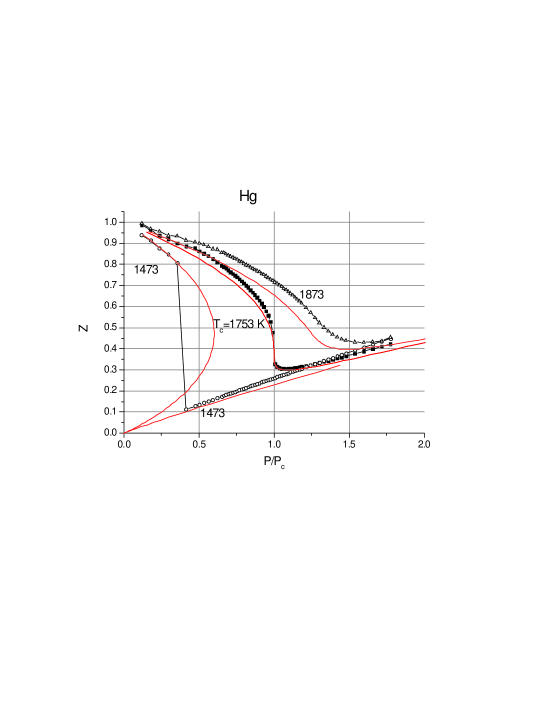
Figure 14: The Hougen–Watson diagram for mercury. Experimental data (from the sources W. Gotzlaff, G. Schonherr, F. Hensel, Z. Phys. Chem. Neue Fol. 156 219 (1988) and W. Gotzlaff., Ph. D. Thesis, University of Marburg, 1988) are equipped with symbols. The thick lines correspond to the van der Waals equation for the related temperatures.

On the other hand, the relation between thermodynamic parameters allows us to decrease the number of independent variables from three to two (cf. Fig. 9 in the variables $\rho,T$ and Figs. 11–16 in the variables $Z,P$).

Estimates.

$\square$ Taking the parameter $\gamma$ into account we use the Euler–Maclaurin formula to obtain

$$\sum_{j}\Big{(}\frac{j^{\gamma}}{e^{bj+\varkappa}-1}-\frac{kj^{\gamma}}{e^{bkj+k\varkappa}}\Big{)}=\frac{1}{\alpha}\int^{\infty}_{0}\Big{(}\frac{1}{e^{bx+\varkappa}-1}-\frac{k}{e^{bkx+k\varkappa}-1}\Big{)}\,dx^{\alpha}+R,$$ (26)

where $\alpha=\gamma+1$, $k=N+1$, $b=1/T$, and $\varkappa=-\mu/T$. Here the remainder $R$ satisfies the estimate

$$|R|\leq\frac{1}{\alpha}\int^{\infty}_{0}|f^{\prime}(x)|\,dx^{\alpha},\qquad\text{where}\quad f(x)=\frac{1}{e^{bx+\varkappa}-1}-\frac{k}{e^{k(bx+\varkappa)}-1}.$$

We calculate the derivative and obtain

$$f^{\prime}(x) =\frac{bk^{2}e^{k(bx+\varkappa)}}{(e^{k(bx+\varkappa)}-1)^{2}}-\frac{be^{bx+\varkappa}}{(e^{bx+\varkappa}-1)^{2}},$$

$$|R| \leq\frac{1}{\alpha b^{\alpha}}\int^{\infty}_{0}\Big{|}\frac{k^{2}e^{k(y+\varkappa)}}{(e^{k(y+\varkappa)}-1)^{2}}-\frac{e^{y+\varkappa}}{(e^{y+\varkappa}-1)^{2}}\Big{|}\,dy^{\alpha}.$$

We also have

$$\frac{e^{z}}{(e^{z}-1)^{2}}=\frac{1}{z^{2}}+\psi(z),\qquad\text{where $\psi(z)$ is a smooth function and $|\psi(z)|\leq C(1+|z|)^{-2}$}.$$

By setting $z=y$ and $z=ky$, we obtain the estimate for $R$:

$$|R| \leq\frac{1}{\alpha b^{\alpha}}\int^{\infty}_{0}\big{|}\psi\big{(}k(y+\varkappa)\big{)}-\psi(y+\varkappa)\big{|}\,dy^{\alpha}$$

$$\leq\frac{k^{-\alpha}}{b^{\alpha}}\int^{\infty}_{k\varkappa}|\psi(y)|\,dy^{\alpha}+\frac{1}{b^{\alpha}}\int^{\infty}_{\varkappa}|\psi(y)|\,dy\leq Cb^{-\alpha}$$ (28)

with a certain constant $C$. For example, if $\varkappa\sim(\log k)^{-1/4}$, then $|R|$ preserves the estimate$|R|\sim O(b^{-\alpha})$. $\square$

The energy will be now denoted by $M$, because without multiplication by the volume $V$, this is not the usual thermodynamics but rather a certain analog of the number theory (see Example 1).

Taking account of the fact that, for the value of $M$, the correction in (2.3) can be neglected for the value of $M$, we obtain

$$M=\frac{\Lambda^{\gamma_{c}-\gamma}}{\alpha\Gamma(\gamma+2)}\int\frac{\xi\,d\xi^{\alpha}}{e^{b\xi}-1}=\frac{\Lambda^{\gamma_{c}-\gamma}}{b^{1+\alpha}}\int_{0}^{\infty}\frac{\eta d\eta^{\alpha}}{e^{\eta}-1},$$ (29)

where $\alpha=\gamma+1$, $b=1/T_{r}$. Therefore,

$$b=\frac{1}{M^{1/(1+\alpha)}}\left(\frac{\Lambda^{\gamma_{c}-\gamma}}{\alpha\Gamma(\gamma+2)}\int_{0}^{\infty}\frac{\xi\,d\xi^{\alpha}}{e^{\xi}-1}\right)^{1/(1+\alpha)}.$$

We obtain (see [70])

$$\sum_{j}\Big{(}\frac{j^{\gamma}}{e^{bj+\varkappa}-1}-\frac{kj^{\gamma}}{e^{bkj+k\varkappa}}\Big{)}=\frac{1}{\alpha}\int_{0}^{\infty}\left\{\frac{1}{e^{b\xi}-1}-\frac{k}{e^{kb\xi}-1}\right\}\,d\xi^{\alpha}+O(b^{-\alpha})$$

$$=\frac{1}{\alpha b^{\alpha}}\int_{0}^{\infty}\left(\frac{1}{e^{\xi}-1}-\frac{1}{\xi}\right)\,d\xi^{\alpha}+\frac{1}{\alpha b^{\alpha}}\int_{0}^{\infty}\left(\frac{1}{\xi}-\frac{1}{\xi(1+(k/2)\xi)}\right)\,d\xi^{\alpha}$$

$$\quad-\frac{k^{1-\alpha}}{\alpha b^{\alpha}}\int_{0}^{\infty}\left\{\frac{k^{\alpha}}{e^{k\xi}-1}-\frac{k^{\alpha}}{k\xi(1+(k/2)\xi)}\right\}\,d\xi^{\alpha}+O(b^{-\alpha})$$

$$= \quad\frac{c(\gamma)}{b^{\alpha}}(k^{1-\alpha}-1)+O(b^{-\alpha}).$$

By setting $k=N|_{\tilde{\mu}/T=0}\gg 1$, we finally obtain

$$N|_{\tilde{\mu}/T=0}\cong(\Lambda^{\gamma_{c}-\gamma}c(\gamma))^{1/(1+\gamma)}T_{r},\quad\text{where}\quad c(\gamma)=\int_{0}^{\infty}\Big{(}\frac{1}{\xi}-\frac{1}{e^{\xi}-1}\Big{)}\xi^{\gamma}\,d\xi.$$ (30)

Corollary 1.

[Erdős formula] It can be proved that $\varkappa\to 0$ gives the number $N$ with satisfactory accuracy. Hence,

$$N_{c}=\int_{0}^{\infty}\bigg{(}\frac{1}{e^{bx}-1}-\frac{N_{c}}{e^{bN_{c}x}-1}\bigg{)}\,dx+O(b^{-1}).$$

Consider the value of the integral (with the same integrand) taken from $\varepsilon$ to $\infty$ and then pass to the limit as $\varepsilon\to 0$. After making the change $bx=\xi$ in the first term and $bN_{c}x=\xi$ in the second term, we obtain

$$N_{c} =\frac{1}{b}\int_{\varepsilon b}^{\infty}\frac{\,d\xi}{e^{\xi}-1}-\int^{\infty}_{\varepsilon bN_{c}}\frac{\,d\xi}{e^{\xi}-1}+O(b^{-1})=\frac{1}{b}\int^{\varepsilon bN_{c}}_{\varepsilon b}\frac{\,d\xi}{e^{\xi}-1}+O(b^{-1})$$ (31)

$$\sim\frac{1}{b}\int^{\varepsilon bN_{c}}_{\varepsilon b}\frac{\,d\xi}{\xi}+O(b^{-1})=\frac{1}{b}\{\log(\varepsilon bN_{c})-\log(\varepsilon b)\}+O(b^{-1})=\frac{1}{b}\log N_{c}+O(b^{-1}).$$ (32)

On the other hand, making the change $bx=\xi$ in (29), we obtain

$$\frac{1}{b^{2}}\int^{\infty}_{0}\frac{\xi\,d\xi}{e^{\xi}-1}\cong M.$$

This gives

$$b=\bigg{(}{\sqrt{M}}\bigg{/}{\sqrt{\int_{0}^{\infty}\frac{\xi\,d\xi}{e^{\xi}-1}}}\,\bigg{)}^{-1},\qquad N_{c}=\frac{1}{2}\frac{\sqrt{M}}{\sqrt{\pi^{2}/6}}\log M(1+o(1))+O(b^{-1}).$$ (33)

Now let us find the next term of the asymptotics by setting

$$N_{c}=c^{-1}M^{1/2}\log c^{-1}M^{1/2}+\alpha M^{1/2}+o(M^{1/2}),\qquad\text{where}\quad c=\frac{2\pi}{\sqrt{6}}\,.$$

Furthermore, using the formula

$$N_{c}=c^{-1}M^{1/2}\log N_{c}+O(b^{-1})$$

and expanding $\log N_{c}$ in

$$\frac{\alpha}{c^{-1}\log c^{-1}M^{1/2}}\,,$$

we obtain

$$\alpha=-2\log\frac{c}{2}$$.

Thus, we have obtained the Erdős formula [71].

The relation $N=T_{r}^{\gamma_{c}+1}\zeta(\gamma_{c}+1)$ is consistent with the linear relation $N=A(\gamma)T_{r}$, where $A(\gamma)=(\Lambda^{\gamma_{c}-\gamma}c(\gamma))^{1/(1+\gamma)}$, for $P_{r}<0$.

We can normalize the activity $a$ at the point $T_{c}$, and we can find $a_{0}$ by matching the liquid and gaseous branches at $T_{c}$ for the pressure $P_{r}=1$, in order to prevent the phase transition on the critical isotherm at $T_{r}=1$.

In what follows, we normalize the activity for $T_{r}<1$ with respect to the value of $a_{0}$ computed below. Then the chemical potentials (in thermodynamics, the thermodynamic Gibbs potentials for the liquid and gaseous branches) coincide, and therefore there can be no “gas–liquid” phase transition at $T_{r}=1$.

Now, for the isochore–isotherm of the “incompressible liquid” to take place, we must construct it with regard to the relation $N_{c}=\zeta(\gamma_{c}+1)$, i.e.,

$$N(T_{r})=T_{r}^{\gamma_{c}+1}\zeta(\gamma_{c}+1).$$

We obtain the value $\gamma(T_{r})$ from the implicit equation

$$A(\gamma)=T_{r}^{\gamma_{c}}\zeta(\gamma_{c}+1).$$

Thus, for each $T_{r}<1$ we find the spinodal curve (i.e., the points at which $\tilde{\mu}=0$) in the domain of negative $\gamma$ [70],

$$\Lambda^{(\gamma-\gamma_{c})/(1+\gamma)}c(\gamma)^{1/(1+\gamma)}=T_{r}^{\gamma_{c}}\zeta(\gamma_{c}+1),$$ (34)

In the set of two values of $\gamma$ corresponding to the solution (34), we choose the value associated with the largest entropy, i.e., the quantity largest in absolute value and denote it by $\gamma(T_{r})$. For $T_{r}=1$, we choose the value of $\Lambda$ so that both solutions $\gamma(1)$ coincide, and we write $\gamma_{0}=\gamma(1)$.

Let $a_{g}=e^{-\mu/T}$ be the activity of the gas, and let $a_{l}=e^{-\tilde{\mu}/T}$ be the activity of the liquid. W e present the condition for the coincidence of $M$ and of the activities at the point of the phase transition:

$$T_{r}^{\gamma_{c}}\operatorname{Li}_{2+\gamma_{c}}(a_{g})=\Lambda^{|\gamma(T_{r})|+\gamma_{c}}T_{r}^{-|\gamma(T_{r})|}\operatorname{Li}_{2-|\gamma(T_{r})|}\left(\frac{a_{l}}{a_{0}}\right),$$ (35)

$$\frac{\Lambda^{\gamma_{c}-\gamma_{0}}}{\zeta(2+\gamma_{c})}\operatorname{Li}_{2+\gamma_{0}}(a_{0})=1,\qquad a_{g}=\frac{a_{l}}{a_{0}}.$$ (36)

Definition 1.

The relation $a_{g}=a_{l}/a_{0}$ will be called the normalization of activity on the critical isotherm.

Relations 35–36 determine the value of the chemical potential $\mu=\tilde{\mu}=T\log a_{g}$ at which the “ gas–liquid” phase transition occurs.

Let $T_{0}=\min_{-1<\gamma<0}A(\gamma)$. Thus, for every $T_{0}<T<T_{c}$, we obtain a value of the reduced activity of the liquid $a_{r}=a_{l}/a_{0}$ ($a_{l}$ is the activity of the liquid) that corresponds to the van der Waals normalization.

Remark 3.

In thermodynamics, the critical values $T_{c}$, $P_{c}$, and $\rho_{c}$ are evaluated experimentally for almost all gases, and therefore the critical number of degrees of freedom can be set in advance. According to numerical calculations for a real gas, the parameter $\lambda=1/\Lambda$ ($1.6<\lambda<3$, $T_{r}>1/3$) determining the point $\gamma_{0}$ ensures that the binodal passes through the triple point (see Sec. 4.4). The triple point can be determined experimentally with a sufficient accuracy.

2.4 Holes in the Bose condensate as observable quantities.
The maximum density of holes

The molecules of an ideal gas can be thought of as tiny balls. Let us imagine holes, excitons in glass, also as balls which are empty, without the substance of a molecule. Obviously, if one mixes these balls in a glass in a chaotic way, then the chaos in the glass becomes increased. This means that the entropy increases in the presence of holes. Therefore, to achieve the maximum of the entropy, we must also additionally mix holes into this glass.

In our conception, holes occur for $\gamma<0$.

In the ideal gas model, we ignore the attraction, and this means that, when “stretching” the liquid, which results in holes, the liquid does not resist (as the sand, which is incompressible under the compression and does not resist under “tension;” cf. the appendix to the book [16]).

Once there is no attraction, there is no negative pressure ‘under the “tension”, i.e., there is no formation of holes. If $\gamma<0$, then the plane $(Z,P)$ is positive again, and therefore it is covered by the other sheet. It can readily be seen that the lines entering the point $Z=0$, $P=0$ (i.e., to the point $\gamma=0$) are reflected on this second sheet back, along the same line. This means that it is geometrically convenient to arrange the reflection of vectors on the second sheet by using the matrix $-I$, where $I$ stands for the two-dimensional identity matrix, i.e., to flip (carry out the mirror reflection for) the sheet $\gamma<0$ to the negative quadrant.

Note that this procedure is compliance with the concepts of Dirac hole theory, just in the opposite direction, namely, to a hole we assign a negative pressure, i.e., a negative energy. Now the straight lines can be continued through the origin to the negative quadrant, although the pressure really does not change its sign. This is only a convenient geometric “uniformization.”

Note also that, due to absence of attraction, an ideal liquid is completely plastic; namely, it does not try to return to the original state (the state before stretching). In this sense, the Bose condensate for $\gamma<0$, which leads to this “kind” of liquid, can also be treated more visually as a glass or an amorphous solid. This makes it possible to interpret the state of the liquid for $\gamma<0$ more intuitively.

Remark 3. The author has come to the revision of the thermodynamics when studying economics in which money is the very particles, according the correspondence principle derived by Irving Fisher. Fisher himself did not referred to his observation as the correspondence principle. However, since he was a disciple of Gibbs, there is a clear reason for the fact that the relation of the basic law of economics

$$PQ=Mv,$$ (37)

where $Q$ stands for the amount of goods, $M$ for the number of money, $v$ for the turnover rate, and $P$ for the price of goods, is obviously related to the correspondence of economical and thermodynamical quantities, namely, the volume $V$ corresponds to the amount of goods $Q$, the number of money $M$ to the number of particles $N$, the rate $v$ to the temperature $T$. The price of goods $P$ is related to pressure to a lesser extent; however, it is denoted by the same symbol.

In this correspondence principle, it is natural to correspond holes to debts and acquitting to annihilation.

As mentioned above, the locus on which the chemical potential is zero gives the points of maximum entropy. We refer to these points as the “new spinodal.” In economics, this new spinodal means a kind of limit for debts [15, 17].

Thus, according to the relations thus obtained, we face a double covering of the plane $\{Z,P\}$ for $\gamma\geq 0$ and $-1\leq\gamma<0$. The meaning of the second sheet is that, for $-1\leq\gamma<0$, the chaotic state of liquid (as a phenomenon associated with the Bose condensate) increases when the number of holes of the type of Frenkel excitons increases, and the holes are placed in the liquid, which is fluctuationally concentrated on a rather slow-moving domain (from the point of view of the device discussed above), in the form of chaotic nanoholes, then the structure of the liquid becomes chaotically stretched.

Here the holes-excitons cannot be indexed by our device, as well as the particles, and we can speak only of the density of holes. As was already said above, it is more convenient to place the second sheet under consideration in the quadrant $[-Z,-P]$, by continuing the straight lines 19 through the singular point of $Z=0$, $P=0$ to the negative quadrant. In other words, to make a reflection with the help of the matrix $-E$, where $E$ stands for the identity matrix.

Thus, it becomes convenient to speak of “ negative pressure”, although we neglect the attraction of particles, and hence there can be no negative pressure at all. As a rule, the pressure, as well as the temperature, is regarded as a positive quantity. We stretch the liquid, and it becomes plastically frozen up in this stretched state and does not tend to shrink back.

Let us explain from the point of view of physics why the extension to the negative square is natural. We compare the new ideal liquid with sand, which is incompressible under the “compression” and “dost not resist” under stretching, because there is no attraction between the grains.

Example 3. Consider a cylindrical vessel, filled with sand, whose lid is attached to the piston, in the room of the space station. The increase in the vessel with the piston leads only to a rearrangement of sand and its transformation to a floating “ dust” in the new volume (see [18]).

If we take into account the gravitational attraction between the grains, then the phenomenon of pulling the piston creates a negative pressure, and thus it is natural to pass to the negative quadrant on the $(P,Z)$ diagram, and then to neglect the gravitational attraction.

Neglecting the presence of attraction here is just as “legitimate” as it is in the theory of vapor-liquid equilibrium, where the condition that the pressures are equal is possible only if we neglect the surface tension.

This also explains a smooth transition (without a phase discontinuity of the first kind) of this structure into ice, namely, a frozen glass crystallizes.

2.5 Critical exponents as observable quantities under the Wiener quantization and the derivation of the Maxwell rule

Mishchenko and the author [19] considered the transition to a two-dimensional Lagrangian manifold in the four-dimensional phase space, where the pressure $P$ and the temperature $T$ (the intensive variables) play the role of coordinates and the extensive variables (the volume $V$ and the entropy $S$) play the role of momenta for the Lagrangian manifold, where the entropy is the action generating the Lagrangian structure.

Seemingly, there is no global canonical transformation leading to a change of this kind. This does not confuse physicists. For example, in §25 of [2], “Equilibrium of a solid in an external field,” it is said that “from the equation

$$dE=TdS+\mu dN,$$ (38)

represented in the form

$$dS=\frac{dE}{T}-\frac{\mu}{T}dN,$$ (39)

we see …”

However, formula 38 does not imply the expression “represented in the form” 39. Nevertheless, this “implies” the following conclusion: “If the field is absent and both $\mu$ and $T$ are constant, then the pressure is automatically also constant.” At the same time, the same textbook states that, at a temperature slightly below the “dew point,” “when the radius of the drop becomes greater than the critical value, it can be seen that the pressure of the liquid inside the drop differs from the pressure in the saturated vapor. The external field is absent. Is this still thermodynamics? Other words are used; one speaks of a vapor instead of gas and of the process of nucleation instead of the vapor-liquid equilibrium. And then a patch is immediately put on the same hole, namely, an extra term is added to 39. The old thermodynamics has many patches of this kind.

It turns out that this complex transformation, leading to relation 39, can be carried out, as we have seen, only by continuing to the domain of negative energies. After this, one can justify the Maxwell transition by introducing a small dissipation (viscosity). The introduction of an infinitesimal dissipation enables one to simultaneously solve the problem of critical exponents, without using the scaling hypothesis, on which the method of renormalization group is based. Let us show this.

In thermodynamics, the viscosity is absent. However, generally speaking, without an infinitesimal dissipation, an equilibrium in thermodynamics should not be attained. Therefore, it is natural to implement the occurrence of this infinitesimal viscosity and then pass to the limit as the viscosity tends to zero.

The geometric quantization of the Lagrangian manifold (see   [20], §11.4) is usually associated with the introduction of the constant $\hbar$. The author introduced the term of Wiener (or tunnel) quantization to describe the case in which the number $\hbar$ is purely imaginary   [21, 22].

Let us apply the Wiener quantization to thermodynamics. The thermodynamic potential $G=\mu N$ is the action $\mathbb{S}=\int p\,dq$ on the two-dimensional Lagrangian manifold $\Lambda^{2}$ in the four-dimensional phase space $q_{1},q_{2},p_{1},p_{2}$, where $q_{1}$ and $q_{2}$ are the pressure $P$ and the temperature $T$, respectively, $p_{1}$ is equal to the volume $V$, and $p_{2}$ is equal to the entropy of $S$ taken with the opposite sign. All other potentials, namely, the internal energy $E$, the free energy $F$, and the enthalpy $W$ are the results of projecting the Lagrangian manifold to the coordinate planes $p_{1},p_{2}$,

$$E =-\int\vec{q}\,d\vec{p},\qquad\vec{q}=\{q_{1},q_{2}\},\quad\vec{p}=\{p_{1},p_{2}\},$$

$$W =-\int(q_{2}\,dp_{2}+q_{1}\,dp_{1}),\qquad F=\int(q_{1}\,dp_{1}-q_{2}\,dp_{2}).$$ (40)

Under the Wiener quantization, we have

$$N=\varepsilon\frac{\partial}{\partial\mu},\qquad V=\varepsilon\frac{\partial}{\partial p},\qquad S=-\varepsilon\frac{\partial}{\partial T}.$$

Consequently, the role of time $t$ in the quantization, is played by $\log(-\mu/T)$,

$$G=\mu N\sim\varepsilon\frac{\mu}{T}\frac{\partial}{\partial(\mu/T)}=\varepsilon\frac{\partial}{\partial\log(-\mu/T)}.$$

Note that the tunnel quantization of the van der Waals equation (vdW) as $\varepsilon\to 0$ gives Maxwell’s rule (see below).

As we shall see below, the critical point and the spinodal point are focal points. and therefore, as $\varepsilon\to 0$ there points do not come to the “classical” picture, i.e., to the van der Waals model. The spinodal points, which are similar to turning points in quantum mechanics, can be approached by the Airy function, whereas the critical point, which is the point at which two turning points are generated (two Airy functions), can be approached by the Weber function (see [23]). It is the very Weber function which is used to express the creation point of the shock wave for $\varepsilon\to 0$ in the Burgers equation is expressed. If one passes to the limit as $\varepsilon\to 0$ outside these points, then we obtain the vdW–Maxwell model. However, the passage to the limit is violated at these very points. Therefore, the so-called Landau “ classic” critical exponents [2] drastically differ from the experiment. The Weber function give singularities of the form $\varepsilon^{-1/4}$, whereas the Airy function gives a feature of the form $\varepsilon^{-1/6}$.

Let us present a more detailed consideration of the Burgers equation.

Consider the heat equation

$$\frac{\partial u}{\partial t}=\frac{\varepsilon}{2}\frac{\partial^{2}u}{\partial x^{2}},\qquad x\in\mathbb{R},\quad t\geq 0,$$ (41)

where $\varepsilon>0$ is a small parameter. As is known, all linear combinations

$$u=\lambda_{1}u_{1}+\lambda_{2}u_{2}$$ (42)

of solutions $u_{1}$ and $u_{2}$ of equation 41 are solutions of this equation.

Let us make the change

$$u=\exp(-w(x,t)/\varepsilon).$$ (43)

We obtain the following nonlinear equation:

$$\frac{\partial w}{\partial t}+\frac{1}{2}\bigg{(}\frac{\partial w}{\partial x}\bigg{)}^{2}-\frac{\varepsilon}{2}\frac{\partial^{2}w}{\partial x^{2}}=0,$$ (44)

which is referred to as the integrated Burgers equation. Obviously, to any solution $u_{i}$ of equation 41 we can assign a solution $w_{i}=-\varepsilon\log u_{i}$ of the equation 44, $i=1,2$. To the solution 43 of equation 41 we assign a solution

$$w=-\varepsilon\log\big{(}e^{-\frac{w_{1}+\mu_{1}}{\varepsilon}}+e^{-\frac{w_{2}+\mu_{2}}{\varepsilon}}\big{)}$$

of the equation 34 where $\mu_{i}=-\varepsilon\log\lambda_{i}$, ($i=1.2$). Since

$$\lim_{\varepsilon\to 0}w=\min(w_{1},w_{2}),$$

we obtain the $(\min,+)$ algebra of the tropical mathematics [24].

To find solutions for $t>t_{\mathrm{cr}}$, Hopf suggested to consider the Burgers equation

$$\frac{\partial v}{\partial t}+v\frac{\partial v}{\partial x}-\frac{\varepsilon}{2}\frac{\partial^{2}v}{\partial x^{2}}=0,\qquad v|_{t=0}=p_{0}(x),$$ (45)

and to refer to the function $p_{\text{gen}}=\lim_{\varepsilon\to 0}v$ (Riemann waves) as a (generalized) solution of the equation

$$\frac{\partial p}{\partial t}+p\frac{\partial p}{\partial x}=0,\qquad p|_{t=0}=p_{0}(x).$$ (46)

The solution $v$ of the Burgers equation can be expressed in terms of the logarithmic derivative

$$v=-\varepsilon\frac{\partial}{\partial x}\log u$$ (47)

of the solution $u$ of the heat equation

$$\frac{\partial u}{\partial t}=\frac{\varepsilon}{2}\frac{\partial^{2}u}{\partial x^{2}},\qquad u|_{t=0}=\exp\bigg{\{}-\frac{1}{\varepsilon}\int_{-\infty}^{x}p_{0}(x)\,dx\bigg{\}}.$$ (48)

Thus, the original problem reduces to the study of the logarithmic limit of a solution of the heat equation. As is known, the solution of problem 48 is of the form

$$u=(2\pi\varepsilon t)^{-1/2}\int_{-\infty}^{\infty}\exp\bigg{\{}-\bigg{(}(x-\xi)^{2}+2t\int_{-\infty}^{\xi}p_{0}(\xi)\,d\xi\bigg{)}\bigg{/}2th\bigg{\}}\,d\xi.$$ (49)

The asymptotics of the integral 49 can be calculated by the Laplace method. For $t<t_{\mathrm{cr}}$, we have

$$u=\big{(}|J|^{-1/2}(\xi(x,t),t)+O(\varepsilon)\big{)}\exp\bigg{\{}-\frac{1}{\varepsilon}{\mathcal{S}}(x,t)\bigg{\}}.$$ (50)

Here

$${\mathcal{S}}(x,t)=\int_{-\infty}^{r(t)}p\,dx,$$

and the integral is evaluated along a Lagrangian curve $\Lambda^{t}$; $r(x)$ is a point on $\Lambda^{t}$. For $t>t_{\mathrm{cr}}$, there are three points $r_{1}(x)$, $r_{2}(x)$, and $r_{3}(x)$ on $\Lambda^{t}$ whose projections to the $x$ axis are the same; in other words, the equation $Q(t,\xi)=x$ for $x\ in(x_{1},x_{2})$ has three solutions $\xi_{1}(x,t)$, $\xi_{2}(x,t)$, and $\xi_{3}(x,t)$.

Write

$${\widetilde{\mathcal{S}}}(x,t)=\int_{-\infty}^{r(x)}p\,dx\quad\text{for}\quad x<x_{1},\quad x>x_{2},$$

${\widetilde{\mathcal{S}}}(x,t)=\min({\mathcal{S}}_{1},{\mathcal{S}}_{2},{\mathcal{S}}_{3})$, and

$${\mathcal{S}}_{j}=\int_{-\infty}^{r_{j}(x)}p\,dx,$$

where $J\in\{1,2,3\}$ for $x\in[x_{1},x_{2}]$.

These arguments enable us to obtain a generalized discontinuous solution of 41 for the times $t>t_{\mathrm{cr}}$. It is defined by a function $p=p(x,t)$ defining the significant areas [21] of the curve   $\Lambda^{t}$. Note that this, in particular, this implies the rule of equal areas, which is known in hydrodynamics for finding the front of a shock wave whose evolution is described by equation 36. Note that this precisely corresponds to the Maxwell rule for the vdW equation.

The solution $v=v(x,\varepsilon)$ of the Burgers equation at the critical point $x=p^{3}$ is evaluated by the formula

$$v(x,\varepsilon)=\varepsilon\frac{\partial\log u(x)}{\partial x}=\frac{\int_{0}^{\infty}\exp\{\frac{-x\xi-\xi^{4}/4}{\varepsilon}\}\xi\,d\xi}{\int_{0}^{\infty}\exp\{\frac{-x\xi-\xi^{4}/4}{\varepsilon}\}d\xi}.$$ (51)

As $x\to 0$, after the change $\frac{\xi}{\root 4 \of{\varepsilon}}=\eta$, we obtain

$$v(\varepsilon,x)\to_{x\to 0}{\root 4 \of{\varepsilon}}\cdot\text{const}.$$ (52)

What does this mean in terms of classical theory and classical measurement, when the condition referred to in the book [1] as the “ semiclassic condition” is satisfied (i.e., for the case in which we are outside the focal point)? For the Laplace transform, this means that we are in a domain in which the Laplace asymptotic method can be applied indeed, i.e., in the domain where

$$u(x)=\frac{1}{\sqrt{\varepsilon}}\int_{0}^{\infty}e^{-\frac{px-\widetilde{S}(p)}{\varepsilon}}\,dp.$$ (53)

If the solution of the relation

$$x=\frac{\partial\widetilde{\mathcal{S}}}{\partial p}$$ (54)

is nondegenerate, i.e., $\frac{\partial^{2}\widetilde{S}}{\partial p^{2}}\neq 0$ at the point at which $\frac{\partial\widetilde{\mathcal{S}}}{\partial p}=x,$ then the reduced integral  53 is bounded as $\varepsilon\to 0$. For this integral to have a zero of the order of $\varepsilon^{1/4}$, we must integrate it with respect to $x$ after applying the fractional derivative $D^{-1/4}$. The value of $D^{-1/4}$ as applied to 1 (the value of $D^{-1/4}1$ is approximately equal to $x^{1/4}$.

By [25, 69], the correspondence between the differentiation operator and a small parameter of the form $D\to 1/\varepsilon$ is preserved for the ratio $-\varepsilon\frac{\partial u/\partial x}{u}$, while the leading term of the asymptotic behavior is not cancelled in the difference between $\frac{\partial^{2}u/\partial x^{2}}{u}$ and $\frac{(\partial u/\partial x)^{2}}{u^{2}}$ due to the uncertainty principle (see Remark 4).

Remark 4. Let us repeat the calculations in [1] with regard to the fact that, on this class of functions, $\overline{D}$ has the properties $\int\varphi D\varphi\,dx=\frac{1}{2}\int D\varphi^{2}\,dx=0$ and $\int x\varphi^{2}\,dx=0.$

Consider the obvious inequality

$$\int_{-\infty}^{+\infty}\bigg{|}ax\psi+\frac{d\psi}{dx}\bigg{|}^{2}\,dx\geq 0,$$ (55)

where $a$ is an arbitrary real constant. When evaluating this integral, we have

$$\int x^{2}|\psi|^{2}\,dx=\overline{(\Delta x)^{2}},$$

$$\int\bigg{(}x\frac{d\psi^{*}}{dx}\psi+x\psi^{*}\frac{d\psi}{dx}\bigg{)}\,dx=\int x\frac{d|\psi|^{2}}{dx}\,dx=-\int|\psi|^{2}\,dx=-1,$$

$$\int\frac{d\psi^{*}}{dx}\frac{d\psi}{dx}\,dx=-\int\psi^{*}\frac{d^{2}\psi}{dx^{2}}\,dx=\frac{1}{\varepsilon^{2}}\int\psi^{*}|D|^{2}\psi\,dx=\frac{1}{\varepsilon^{2}}\overline{|\Delta D|^{2}}.$$ (56)

We obtain

$$a^{2}\overline{(\Delta x)^{2}}-a+\frac{1}{\varepsilon^{2}}\overline{|\Delta D|^{2}}\geq 0.$$ (57)

For this quadratic trinomial (in $a$) to be positive for all values of $a$, it is necessary that the following condition be satisfied:

$$4\overline{(\Delta x)^{2}}\frac{1}{\varepsilon^{2}}\overline{|\Delta D|^{2}}\geq 1$$

or

$$\sqrt{\overline{(\Delta x)^{2}}\ \overline{|\Delta D|^{2}}}\geq\frac{\varepsilon}{2}.$$ (58)

Thus, the tunnel quantization explains both the condition $\mu=0$ for photons and the condition $\mu\leq 0$ for bosons.

In the case of thermodynamics, the role of $x$ is played by the pressure $P$, and the role of the momentum $p$ is the played by the volume $V$. Therefore, $V\sim P^{1/4}$, i.e.,

$$P_{c}\sim(V-V_{c})^{4}.$$ (59)

This is the very jump of the critical exponent. One van similarly obtain other critical exponents (see [25]). For the comparison with experimental data, see the same paper.

Unfortunately, thermodynamics does not use the concept of Lagrangian manifold which was introduced by the author in 1965 [26]. It is especially suitable for thermodynamics, in which there are pairs of intensive and extensive quantities. Intensive quantities, roughly speaking, are the quantities for which one cannot create the concept of “specific” quantity. These are the temperature $T$, the pressure $P$, and the chemical potential $\mu$. To these intensive quantities, there correspond related extensive quantities, namely, the entropy $S$, the volume $V$, and the number of particles $N$. Altogether, they form the phase space, where the role of coordinates is played by the intensive quantities and the role of momenta is played by the extensive quantities. In this case, a Lagrangian manifold is a three-dimensional submanifold (of the six-dimensional phase space) on which there is an action, an analog of the integral ${\mathcal{S}}=\int p\,dq,\qquad q\in\mathbb{R}^{2}$, $p\in\mathbb{R}^{2}$ in mechanics. It is locally independent of the path.

Usually a 4-dimensional phase space $T,S;P,V$ is considered. This space corresponds to $q\in R^{2},p\in R^{2}$, $q_{1}\to T$, $q_{2}\to P$, $p_{1}\to S$, $p_{2}\to V$: $d{\mathcal{S}}=p_{1}\,dq_{1}+p_{2}\,dq_{2},$ depending on the coordinate plane of the form $q_{1},q_{2}$; $q_{1},p_{2}$; $p_{1},q_{2}$; $p_{1},p_{2},$ to which the Lagrangian manifold is projected.

The Lagrange property means that the number of planes cannot coincide (there are no planes of the form $q_{1},p_{1}$ and $q_{2},p_{2}$). To every projection there corresponds some potential ($q_{1},q_{2}$ is the thermodynamic potential, etc.).

This is an obvious correspondence. If it were more elaborated, then, on one hand, the transition from the action $d{\mathcal{S}}=p_{1}\,dq_{1}+p_{2}\,dq_{2}$ to the “action”–coordinate $dq_{1}=d{\mathcal{S}}/p_{1}-(p_{2}/p_{1})\,dq_{2}$ would be not “so obvious” (see formulas 28–29). On the other hand, it would be natural to use the semiclassical (Wiener–Feynman) quantization of action rather than the scaling hypothesis.

(The quantization of the Lagrangian manifold differs from the full quantization of thermodynamics [27] in the same way in which the semiclassical Bose–Sommerfeld geometric quantization differs from the quantization of Schrödinger, Heisenberg, and Feynman.

The term “dequantization,” which is well-known in the tropical mathematics [24], means the Wiener or tunnel quantization of the Lagrangian manifold, and then the passage to the limit as the quantization parameter (the viscosity) tends to zero.

3 Nuclear physics in nano scale

3.1 Rotation of a neutron in the coat of Helium-5

In [28], [29], the author introduced a hidden parameter $t_{\mathrm{meas}}$ (measurement time) binding together quantum and classical mechanics. The author considered this parameter using helium-4, helium-5, and helium-6 as examples. A detailed proof of the theorem involving the hidden parameter for helium-5 invokes a considerable number of auxiliary statements and theorems. The author, essentially, proved and discussed all these auxiliary statements, such as approximations based on the Hartree equation in the case of the Bose distribution in his earlier papers (see [30], [51]). In particular, the author obtained a rigorous correction to the Stefan–Boltzmann law [31] and proved that the formal series defining the succeeding terms are false. In Gentile statistics (parastatistics) [32], the author also obtained a number of estimates and lemmas (see for example, [33]–[36]).

In the present Section, we present only a scheme of proof of the applicability of the hidden parameter $t_{\mathrm{meas}}$ introduced by the author [37] for explaining the behavior of the neutron in the coat of helium-5. The detailed proof is contained in the asymptotics obtained by the author earlier. Here we shall present the material in such a way as, on the one hand, to make it accessible to mathematicians who studied the author’s papers and, on the other hand, to make it clear to nuclear physicists.

The parameter under discussion in this paper is not hidden in the sense that was attributed to it by the authors of the Einstein–Podolsky–Rosen paradox (EPR). This parameter is a completely natural and clear parameter. In the quotation from the book [1] dealing with the identity of the particles often referred to in the author’s papers, this parameter is veiled: this is the “instant of time,” at which the numbering of particles is achieved. They wrote: “the particles belonging to a given physical system can be considered as ‘numbered’ at some instant of time [1, p. 252 of the Russian edition].” It is the time during which the particles were numbered that was introduced as an additional parameter in [28], [29], [37] and which is considered in the present paper. This time depends on the algorithm used for the numbering of particles. The time needed for the operation of the algorithm, in turn, depends on the computing facilities. Thus, this parameter is not hidden, but is veiled; it can be determined exactly only under a large number of additional conditions.

1. The self-consistent equations obtained by the author, were first given in [15]. They relate the Gentile statistics with the Bose-Einstein statistics and the Fermi-Dirac statistics:

$$N =VT^{\gamma+1}(\operatorname{Li}_{1+\gamma}(a)-\frac{1}{(N^{\alpha}+1)^{\gamma}}\operatorname{Li}_{1+\gamma}(a^{N^{\alpha}+1})),$$ (60)

$$M =VT^{\gamma+2}(\operatorname{Li}_{2+\gamma}(a)-\frac{1}{(N^{\alpha}+1)^{1+\gamma}}\operatorname{Li}_{2+\gamma}(a^{N^{\alpha}+1})),$$ (61)

where the $M=\Omega$ is the potential, $\Omega=-VP$, $P$ is the pressure, $V$ is the volume, $T$ is the temperature, $a$ is the activity, and $D=2\gamma+2$ is the number of degrees of freedom. The value of $\alpha$ varies from $1$ to $0$.

The case in which we set $N\log(a)\to 0$ in the macroscopic equations (60)–(61), belongs to mesoscopic physics. In thermodynamics, this situation arises near the point of change of the sign of the activity $a$, i.e., near the point of passage of the Bose–Einstein distribution to the Fermi–Dirac distribution (for $\gamma\leq 0$).

Remark 4.

It is well known that thermodynamics can be carried over to economics. Thus, Irving Fisher associated the price of goods with the quantity $PV$ and the amount of money with the number of particles $N$. The author associated the amount of debts with the negative values of $N$. In economics, $N=0$ or $N<0$ are regarded as a day-to-day usual situation.

We introduce the notation $W=V(\lambda^{2}T)^{\gamma+1}$, and let $\lambda$ be the parameter depending on the mass. In number theory, $\gamma=0$ and $\lambda=1$ [36].

Here we apply Gentile statistics (parastatistics) and relate it, in a self-consistent way, to the statistics of bosons and fermions in mesoscopic physics.

Figure 6A: Numerically found exact dependence of $N$ on $a$. The solid curves correspond to $\gamma=0$, $\lambda=1$, $W=1000$, $\alpha=0.5,0.8,0.9,0.9999$ (from left to right). The points correspond to $\alpha=1$ because of two reflections. The dotted curve corresponds to $N=-1/\log(a)$.

Consider the case in which $N_{i}$ is the number of holes. This means that we assume $N_{i}$ to be a negative number. Then

$$\sum(-N_{i})=-N,\qquad-\sum\varepsilon_{i}N_{i}=-M.$$ (62)

Thus, the numbers $-N$ and $-M$ are also negative. The multiplication of both equalities by -1 leads to the same case in which the $N_{i}$ are positive. Therefore, the formulas of Gentile statistics remain the same. This means that, in the formulas of Gentile statistics, we can replace the numbers $N$ and $M$ by their absolute values. In this way, we can extend Gentile statistics to negative numbers $N_{i}$, i.e., to the case of holes.

To extend the self-consistent formulas of the statistics introduced by the author in [15] to the case of “holes,” we must extend the curves given in Fig. 6A into the negative domain, using their mirror reflection in the axis $a$ (see Fig. 7A).

Remark 5.

If we use the mirror reflection of the appropriate curve with respect to the line $a=a_{0}$, where $a_{0}$ satisfies the equation $N(a_{0})=0$, then the curve will be a continuously differentiable continuation of the original curve describing the self-consistent equation for $N>0$. The second derivative undergoes a jump.

Definition 2.

The distance from the point $a=0.00010$, where $\alpha=0$, $N=0$, to the intersection point with the curve $N=1/\log(a)$ is called the spin concentration.

This concentration plays a role similar to $\Delta m$ in Einstein’s formula $E=\Delta mc^{2}$, where $c$ is the velocity of light  [39].

Our expansion in the small parameter $N\log(a)$ will bound the curve described above by its intersection point with the line $N=1/log(a)$. At this point, as is seen from Fig. 6A, the $\Omega$-potential attains its largest absolute value on the closed interval $|N|=|1/\log(a)|$.

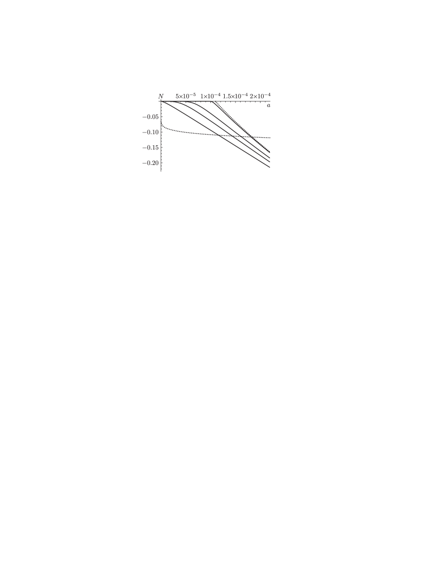
Figure 7A: The reflection of the curves $N(a)$ depicted in Fig. 6A with respect to the line $N=0$. The solid curves correspond to $\gamma=0$, $\lambda=1$, $W=1000$, $\alpha=0.5,0.8,0.9,0.9999$ (from left to right). The points correspond to $\alpha=1$ in view of two reflections. The dotted curve corresponds to $N=-1/\log(a)$.

In the positive domain of energy, the curves $\alpha=0.5,0.8,0.9,1$ are symmetric with respect to the axis $a$; hence a similar jump in the energy occurs also in the positive domain of energy. Thus, particles from the positive domain jump into the symmetric negative domain.

To the author’s knowledge, such an energy jump in a transition occurs in thermodynamics only in the quantum case and in the case of a capillary with superfluid helium-4 at the point at which the Allen–Jones spouting occurs [40]. Therefore, in our case, we can assume that, at the point of passage of the Einstein–Bose distribution to the Fermi–Dirac distribution a similar “spouting” on a mesoscopic scale occurs. In our case, the Allen–Jones “spouting” is the phenomenon in which one neutron breaks away and goes to infinity with the velocity obtained in the energy jump.

Let us pass to the model of the helium nucleus. According to Bohr, the nucleons inside the shell of the nucleus do not interact (there is no attraction between them). They act as colliding balls. Indeed, according to the latest experiments, nucleons attract to one another only at distances less than or equal to their radii.

But this fact is also an approximation. Indeed, by the Schrödinger equation, the nucleon is a wave packet. Therefore, it spreads from its original $\delta$-shaped structure and, therefore, there is a small interaction $\varepsilon V(x-y)$ between nucleons. Here $\varepsilon$ is a small parameter, $x$ corresponds to one nucleon and $y$ to the other, and $V(x-y)$ is the interaction potential. The parameter $\varepsilon$ is a “ hidden” parameter. For $\gamma>0$, the number of degrees of freedom depends on the relationship between this parameter and the Planck constant.

This implies the following:

(1) the maximum number of degrees of freedom of the nucleon is $6n-5$, where $n$ is the number of nucleons ([2, Sec. 44]);

(2) by the self-consistent Hartree equation for fermions and bosons, the interaction potential $\varepsilon V(x-y)$ for helium-4 constitutes a double shell—the first shell with a high barrier and the second shell with a low barrier. The first shell contains two neutrons and two protons, while the second shell contains two neutrons for at most 1 s, forming helium-6. We can state conditionally that, outside this time interval, between the main (first) shell and the second shell, there are two “holes,” which, occasionally, are filled by neutrons.

The distance between the two shells constitutes the so-called coat. The given construction refines the initial Bohr model in which the nucleons do not attract one another.

We obtained the following relation for $W=V(\lambda^{2}T)^{\gamma+1}$

$$W=\frac{E_{\mathrm{nuc.bin}}}{T_{c}\zeta({2+\gamma})(\gamma+1)},$$

where $E_{\mathrm{nuc.bin}}$ is the nuclear binding energy. For helium-4, the value of $W$ turns out to be $3.1\times 10^{10}$. At the intersection point of the graphs $N=-1/\log(a)$ and $N(a)$ (see Fig. 8A), the energy $E$ is $0.12\ T_{c}$ or $53.1\times 10^{-6}$ eV .

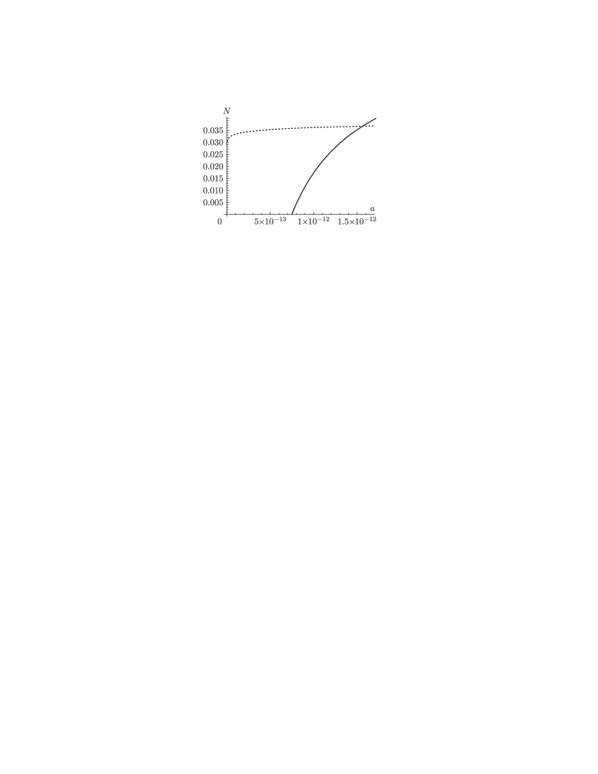
Figure 8A: The solid line corresponds to the dependence $N(a)$; the dashed line describes the function $N=-1/\log(a)$. Here $\gamma=0.5$, $\lambda=1$ $W=4.7\cdot 10^{10}$.

Hence, by defining

$$t_{\mathrm{meas}}=\hbar/E_{\mathrm{ms}},$$

we obtain $t_{\mathrm{meas}}=1.24\times 10^{-11}$ s. For $\gamma=2.5$, the mesoscopy (the number of particles is less than $10^{6}$) passes into a microscopy (the number of particles is 2).

In the above-mentioned paragraph from the book [1], Landau and Lifshits wrote about another instants of time: if “in the following time, one observes the motion of each particle along its own trajectory, then, at any instant of time (italicized by me—VM), the particles can be identified.”

Note that the time during which the experimenter sees the behavior of the particles is much less than the time $t_{\mathrm{meas}}$ of the experiment (of the numbering) (and at least 100 times less than the lifetime of the fermion of helium-5). Instants of time constitute a discrete collection of points. If the time intervals between these points are much less than the veiled parameter, then the observer will see the classical pattern of rotation of the neutron (of the wave packet) about the nucleus of helium-4 regardless of the lifetime of the fermion of helium-5.

3.2 Nuclear decay

The development of wave mechanics started from de Broglie’s paper “Ondes et quanta” in 1923. De Broglie considered the motion of electron in a closed orbit and showed that the requirement that the phases be consistent results in the Bohr–Sommerfeld quantum condition, i.e., to the quantization of the angular momentum. In 1927, developing his ideas about the relation between waves and particles, de Broglie constructed the theory of double solution [41] which, in fact, resulted in the well-known notion of wave-corpuscle dualism, which is still actual nowadays.

De Broglie concluded that the presence of a continuous wave is related to the fact that the Lagrangian of the particle contains an additional term which can be treated as a small addition of the potential energy (cf. formula (69) below). This theory agrees well with the so-called Bell inequalities [42] and is a nonlocal theory.

a. Bose statistics and Fermi statistics in the Hougen–Watson diagrams and in the Gentile statistics

Bohr and Kalckar investigated the boson nucleus [43]. The capture of one neutron turns the boson nucleus into a fermion.

The behavior of Bose and Fermi particles is described by the Bose–Einstein and Fermi–Dirac distributions, respectively. The Bose–Einstein distribution in polylogarithm form becomes

$$\operatorname{Li}_{s}(a)=\frac{1}{\Gamma(s)}\int_{0}^{\infty}\frac{t^{s-1}}{e^{t}/a-1}\,dt,$$ (63)

where $\operatorname{Li}_{(\cdot)}(\cdot)$ is a function of the polylogarithm. The Fermi–Dirac distribution can be written as

$$-\operatorname{Li}_{s}(-a)=\frac{1}{\Gamma(s)}\int_{0}^{\infty}\frac{t^{s-1}}{e^{t}/a+1}\,dt.$$ (64)

We consider the quantum particles each of which is associated with a wave packet. These wave packets are related to the de Broglie thermal wavelength $\Lambda$.

Assume that $a=e^{\mu/T}$ is the activity ($\mu$ is the chemical potential), $s=D/2$, and $D$ is the number of degrees of freedom (dimension). We denote the total energy of all $N$ particles (molecules) by $E$.

One can see that, for the activity $a$ changing sign, the distributions (63) and (64) themselves also change sign. This corresponds to the transition from negative pressures to positive pressures. In the van der Waals formulas [44], [45], such a picture is rather natural. Thus, the fermions and bosons are located in different quarter on the Hougen–Watson PZ-diagram ($P$ is the pressure, $Z=PV/(NT)$ is the compressibility factor, where $V$ is the volume, $N$ is the number of particles, and $T$ is the temperature): the bosons are in the negative domain and the fermions are in the positive domain. Developing the Bohr–Kalckar approach to the relation between the nucleus model and formulas of decomposition of an integer into terms (see the work [43] mentioned above), the author showed that this phenomenon is also manifested in diagrams of the number theory [46].

b. Gentile statistics

In physics, the Bose–Einstein and Fermi–Dirac distributions are determined by using the Gentile statistics [32]. The Gentile statistics comprises the Bose statistics and the Fermi statistics are particular cases. The Gentile statistics contains an additional constant $K$ which denotes the maximal number of particles located at a fixed energy level. In particular, for $K=1$, the distributions of the Gentile statistics coincide with the distributions of the Fermi–Dirac statistics, i.e., the formulas coincide with (64) in form. In the Gentile statistics, one assumes that $K\geq 1$.

Considering the $\Omega$-potential corresponding to the Gentile statistics, we can obtain a detailed description of the boson-to-fermion transition. And judging by analogy with the $\Omega$-potential considered by Landau and Lifshits [2], this allows one to calculate the energy of this transition. In [2], for the case $s=3/2$, the following formula for the total energy of gas is given:

$$E=\int_{0}^{\infty}\varepsilon\,dN_{\varepsilon}=\frac{gVm^{3/2}}{\sqrt{2}\pi^{2}\hbar^{3}}\int_{0}^{\infty}\frac{\varepsilon^{3/2}\,d\varepsilon}{e^{(\varepsilon-\mu)/T}-1}.$$ (65)

The fermions in the boson are “experimentally” indistinguishable: if two fermions constituting a boson are interchanged, then these states cannot be distinguished experimentally. If a boson splits into two fermions that can be distinguished, they cannot interchange their places and transform into each other. One can say that the fermions are experimentally distinguishable or indistinguishable depending on whether the experiments permit distinguishing the fermions comprising the boson.

Our goal is to determine the total energy of transition of a boson consisting of two experimentally indistinguishable fermions into two distinguishable fermions. This transition occurs in the following two stages: the transition from indistinguishable fermions (boson) to the distinguishable fermions and then the disappearance of a fermion. As a result, the processes reduces to the transition of formula (63) into formula (64).

c. Notation

Let us introduce the new notation which permits determining the energy in dimensionless form.

Let $\mathfrak{v}=\Lambda^{2s}$. This quantity has the dimension of volume in the $2s$-dimensional space. Let $\mathbf{E}=\frac{2\pi\hbar^{2}}{m}{V}^{-\frac{1}{s}}$. This quantity has the dimension of energy .

Now we introduce dimensionless variables, $\mathfrak{E}={E}/{\mathbf{E}}$ for the total energy and $\mathfrak{V}={V}/{\mathfrak{v}}$ for the volume. We note that the quantity $\mathfrak{V}^{1/D}$ is the ratio of the characteristic linear dimension of the system ${V}^{1/D}$ to the de Broglie wavelength $\Lambda$.

Usually, $N_{i}$ denotes the number of particles located at the $i$th energy level. It is assumed that, in the case of the Fermi gas, there is at most one particle at each energy level, and in the case of the Bose gas, the number of particles $N_{i}$ at each energy level can be arbitrarily large. We consider the Gentile statistics [32] according to which, at each energy level, the number of particles located at each energy level is bounded by the number $K$. In other words, the number of particles at any energy level cannot exceed the number $K$.

The maximal number of particles at an energy level in the system is attained for the maximal value of the activity $a$, i.e., at the point $a=1$. Since $\sum_{i=1}^{M}N_{i}=N$, it is obvious that $N_{i}\leq N$ for the Bose system. Therefore, $K\leq N$ for the Bose system. In the Gentile statistics, the $K$ are integers such that $K_{i}<K_{i+1}$.

We assume that $K=N$ in an infinitely small neighborhood of $[N]$, where $[N]$ is the integral part of the number $N$.

In the nonstandard analysis developed by Robinson (see [47]–[48]), the set of points infinitely close to the number $[N]$ is called the Leibnitz differential [49] which is understood as the length of an elementary infinitely small interval (monad). The differential is an arbitrary infinitely small increment of a variable.

By $x$ we denote the difference $N-[N]$, i.e., $N-[N]=x>0$. We seek the expansion in a power series in $x$ up to $O(x^{2})$, which implies that $N\sim[N]$.

For the ideal gas of dimension $D$ obeying the Gentile statistics, i.e., in the case where, at each energy level, there can be at most $K$ particles ($K$ is an integer), the following relation for the number of particles $N$ is known:

$$N=\mathfrak{V}(\operatorname{Li}_{s}(a)-\frac{1}{(K+1)^{s-1}}\operatorname{Li}_{s}(a^{K+1})).$$ (66)

The self-consistent relation for $x$ in a neighborhood of $[N]$ has the form

$$[N]+x=\mathfrak{V}(\operatorname{Li}_{s}(a)-\frac{1}{([N]+x+1)^{s-1}}\operatorname{Li}_{s}(a^{[N]+x+1})).$$ (67)

The following thermodynamical formula for the energy is known:

$$\mathfrak{E}=s\mathfrak{V}^{\frac{s+1}{s}}(\operatorname{Li}_{s+1}(a)-\frac{1}{([N]+x+1)^{s}}\operatorname{Li}_{s+1}(a^{[N]+x+1})).$$ (68)

We note that, in the thermodynamics, $N$ is the number of molecules. In this paper, we do not consider molecules, we only consider the nucleus, i.e., the nuclear physics. In this sense, we can speak that, in our model, the number of molecules $N$ is zero. Therefore, in contrast to the standard Gentile statistics, we also assume that $K=0$, and we consider only the case $[N]=0$. To the numbers $N=K=0$ we apply the nonstandard analysis and the technique of the Gentile statistics [32].

Using the technique of nonstandard analysis, we add a monad $x$ to the integer $K$. Then expression (66) is not equal to zero.

We expand the right-hand side of Eq. (67) in small $x\neq 0$ omitting the third-order terms:

$$\begin{split}&x=\mathfrak{V}x((s-1)\operatorname{Li}_{s}(a)-\log(a)\operatorname{Li}_{s-1}(a))\\ &+\mathfrak{V}\frac{1}{2}x^{2}\left(\log^{2}(a)(-\operatorname{Li}_{s-2}(a))-(s-1)(s\operatorname{Li}_{s}(a)-2\log(a)\operatorname{Li}_{s-1}(a))\right),\end{split}$$ (69)

Cancelling $x$ in both sides of (69) and passing to the limit in (69), $x\to 0$, we obtain an expression for $a_{0}$, i.e., the value of $a$ at which $N=0$:

$$(s-1)\operatorname{Li}_{s}(a_{0})-\log(a_{0})\operatorname{Li}_{s-1}(a_{0})-\mathfrak{V}^{-1}=0.$$ (70)

The value $\operatorname{Li}_{s}(a)$, where $a=e^{\mu/T}$, is associated with the total energy of transition, in particular, in the three-dimensional case ($s=3/2$).

We note that it follows from Eq. (70) that, $a_{0}\to 0$ as $\mathfrak{V}\to{\infty}$. This means that the values $a_{0}$ are small in the case where the value of the system characteristics linear dimension, which is equal to ${V}^{1/D}$, exceed the de Broglie thermal wavelength $\Lambda$.

For a sufficiently large value $\mathfrak{V}=\frac{V}{\Lambda^{2s}}$, Eq. (70) has a unique solution $a_{0}\leq 1$ which depends on $\frac{V}{\Lambda^{2s}},s$. We have

$$(s-1)\operatorname{Li}_{s}(a_{0})-\log(a_{0})\operatorname{Li}_{s-1}(a_{0})=\frac{\Lambda^{2s}}{V}.$$ (71)

The expression for the de Broglie thermal wavelength $\Lambda$ has the form $\Lambda=\sqrt{\frac{2\pi\hbar^{2}}{mT}}$.

The value of the activity $a$ at a known temperature $T$ determines the following value of the chemical potential $\mu$:

$$\mu=T\log(a)\leq 0.$$ (72)

In particular, at $a=a_{0}$, the greater the temperature $T$, the less $a_{0}$ and the greater the corresponding value $|\mu_{0}|$. Thus, as the temperature increases, the transition point $\mu_{0}$ approaches the point $\mu=-\infty$ at which the pressure $P$ changes sign.

Assume that $a_{0}=1$ and the mass $m$ and the volume $V$ of the nucleus are known. Then, taking the expression for the de Broglie thermal wavelength $\Lambda=\sqrt{\frac{2\pi\hbar^{2}}{mT}}$ into account, we can consider Eq. (71) as an equation for $T$.

The temperature arising at $a=1$, i.e., as $\mu\to 0$, will be called the critical temperature. We denote it by $T_{s}$. Since the temperature $T_{s}$ is the lowest on the whole interval of variation in $\mu$ which is the ray $(-\infty,0]$, the ratio $T/T_{s}$ will be called the regularized temperature, and we denote it by $T_{\text{reg}}$. The temperature variation along the isotherm can be measured in $T_{\text{reg}}$.

The expansion of the energy (68) in small $x$ up to the first order inclusively has the form

$$\mathfrak{E}=s\mathfrak{V}^{\frac{s+1}{s}}x(s\text{Li}_{s+1}(a)-\log(a)\text{Li}_{s}(a)).$$ (73)

The ratio of the total energy $\mathfrak{E}$ to the number $x$ will be called the nonstandard specific energy. Let us calculate the nonstandard specific energy at the point $a_{0}$ of boson-to-fermion transition.

Thus, at the point $a=a_{0}(\mathfrak{V},s)$, the values of the nonstandard specific energy $\mathfrak{E}_{sp0}$ and ${E}_{sp0}$ are expressed by the formulas

$$\mathfrak{E}_{sp0}(\mathfrak{V},s)=s\mathfrak{V}^{1+1/s}(s\operatorname{Li}_{s+1}(a_{0})-\log(a_{0})\operatorname{Li}_{s}(a_{0})),$$ (74)

$${E}_{sp0}(\mathfrak{V},s,T)=s\mathfrak{V}T(s\operatorname{Li}_{s+1}(a_{0})-\log(a_{0})\operatorname{Li}_{s}(a_{0})).$$ (75)

We note that the dimensionless nonstandard specific energy $\mathfrak{E}_{sp0}$ depends on the two variables $\mathfrak{V}$ and $s$, while the dimensional nonstandard specific energy ${E}_{sp0}$ depends already on three variables $\mathfrak{V}$, $s$, and $T$, where $T$ is also a dimensional variable.

We have considered above the behavior of the Bose–Einstein distribution in a neighborhood of the point $a=0$ and showed that the decay of a boson into two fermions occurs at the point $a=a_{0}$ different from zero. Then, using an analog of the Gentile statistics for $K=0$, we calculated the value of the nonstandard specific energy required for the transition of a boson into two fermions. Despite the fact that the Gentile statistics was previously applied to the number of particles greater than $1$, the use of the nonstandard analysis (Leibnitz differential or monads) allowed the author to generalize the Gentile statistics relations to the case of a small number of bosons for $N=K=0$.

Thus, using mathematical tools, we showed that the application of Gentile statistics to monads allows one to obtain an approximate answer for the problem of determining the nonstandard specific energy of transition of a boson into two fermions.

The notion of wave packet means that a particle is not a point, but it is spreading. This process depends on the thermal wavelength of de Broglie wave packets. If we consider the $\mathfrak{V}$-functions corresponding to nucleons which are related to the quarks through the variables in the symmetry groups with a large number of degrees of freedom, then the number of variables can significantly increase. In this case, one can associate quantum mechanical particles with monads of nonstandard analysis

4 Considering the attraction.
Dimers (pairs) as observable quantities

4.1 Second quantization of classical mechanics and ultrasecond quantization of thermodynamics. Operators of creation and annihilation for pairs-dimers

The second quantization is always associated with the identity of particles, and, if it is carried out for classical particles, then it is tacitly assumed that the particles are indistinguishable for the observer. Instead of an $N$-dimensional problem, we arrive at the three-dimensional picture in which $N$ particles are distributed. The Vlasov equation [50, 51] is obtained from the second quantization of classical mechanics. However, the original arguments used by Vlasov were actually based on the assumption that the particles can be regarded as identical ones.

In the classical system of Hamilton equations for $N$ particles, even if the Hamiltonian is invariant under any permutation of the particles, the initial conditions need not have this property. However, the initial conditions of the Liouville equation can be regarded as data satisfying the conditions of symmetry.

Indeed, let

$$\{q_{i}^{0},p_{i}^{0}\},\qquad(q_{i}^{0}=q^{0}_{i,1},q^{0}_{i,2},q^{0}_{i,3},\qquad p_{i}^{0}=p_{i,1}^{0},p_{i,2}^{0},p_{i,3}^{0})$$ (76)

are initial conditions for the Hamiltonian system whose Hamiltonian is invariant under every permutation $p_{i},p_{j}$ and also under every permutation $q_{i},q_{j}$. For example, let

$$H(p,q)=\sum\frac{p_{i}^{2}}{2m}+\sum\sum V(|q_{i}-q_{j}|).$$ (77)

Substituting the initial conditions into the Hamiltonian 77, we obtain the energy

$$E=H(p^{0},q^{0}).$$ (78)

The energy is conserved along the trajectories of the Hamiltonian system.

Consider further the Liouville equation corresponding to the Hamiltonian system

$$\frac{\partial\rho}{\partial t}=\{H(p,q),\rho\},$$ (79)

where $\{\cdot\}$ stands for the Poisson bracket, with the initial condition

$$\rho(E),\qquad\rho(E)\in C^{\infty},$$

where $E$ satisfies 78. This equation describes the distribution corresponding to the Hamiltonian system with the initial conditions given above.

The Liouville equation and the initial conditions are symmetric with respect to any transposition of $p_{i}$ and $p_{j}$ and to any transposition of $q_{i}$ and $q_{j}$. This symmetry is preserved for the solutions. According to the Gibbs distribution for the Gibbs Ensemble, every distribution can be expressed in terms of energy. Therefore, it is symmetric with respect to any permutation of the particles.

Schönberg [52] carried out a second quantization of this system in the Fock space. In [51], the Vlasov equation was obtained under the assumption that the interaction is small and the number of particles is large. The BBKKI chains are also symmetric with respect to these permutations. Hence, for any distribution in the many-body problem, such a symmetry follows. Thus, we arrive at the invariance with respect to the permutations of the particles, and thus to a “distribution of Bose–Einstein type” for the statistical physics of classical particles. Other mathematically rigorous arguments which lead to a “distribution of Bose–Einstein type,” in the form of lemmas and theorems (see [53]), and hence also the distributions of classical particles, obey the laws of number theory.

Although a modern macroinstrument cannot trace the motion of every particle (because of discreteness of the observation times in relaxationally stepwise process), which is possible at the classical level, but it can distinguish between molecules and dimers or clusters. The clusters consisting of more than two molecules occur in gas much less frequently than dimers. Dimers are observable at all temperatures, and a macroinstrument can calculate their average percentage at a given temperature. This is an important new phenomenon in experiment, and this phenomenon was not available to the great who formulated the basic laws of thermodynamics.

Dimers occur and become immediately split by monomers (single molecules), and they are created and annihilated in different places. They occur because there are quantum forces of attraction between molecules (the dipole-dipole interaction). The dimers are virtual, as the ideal liquid is.

To take into account this important phenomenon (the creation and annihilation of dimers) mathematically, one obviously needs to make the “second” quantization and introduce the creation and annihilation operators for dimers, i.e., for pairs. The author referred to this “second” quantization as the “ultrasecond” quantization due to the introduction of creation and annihilation operators for pairs. In the special case of the Bardeen model, this quantization was introduced in essence [54],  [51]; however,since this model is, roughly speaking, exactly solvable, these operators turned out to be hidden in the model in a sense.

In general, the ultrasecond quantization and the asymptotic behaviors associated with it are rather cumbersome and lead to quantum equations involving the Planck constant $\hbar$. The passage to the limit as $\hbar\to 0$, and then the passage to the limit as the viscosity tends to zero, are cumbersome, and we present here only a part of this passage, which is related, as in the previous section, with the introduction of an infinitesimal viscosity into the classical scattering problem (for $\hbar=0$ ). This means that we introduce the viscosity and, after manipulations, pass to the limit as the viscosity tends to zero. This procedure will enable us to find the Boyle temperature $T_{B}$, and then also the Boyle density $\rho_{B}$, i.e., the so-called Zeno line, which is present in the van der Waals model and which was first noticed by Bachinski in experiments with pure gases.

We shall further obtain the so-called law of corresponding states.

4.2 Boyle temperature as the temperature above which the dimers are not observable in the Boltzmann–Maxwell ideal gas

The attraction between the particles occurs in the quantum mechanical consideration of the dipole-dipole interaction. In the standard semiclassical limit, if the distance between neutral molecules is fixed (does not depend on the parameter $\hbar$, i.e., on a dimensionless parameter proportional to $\hbar$), then, as $\hbar\to 0$, the attraction disappears. In this sense, the use of an attraction potential in molecular dynamics using the classical Newton equations for many particles is at least baseless.

However, if, along with $\hbar$, the problem involves other small and large parameters, then the attraction potential can be kept for some relationships among these parameters under the passage to the limit as $\hbar\to 0$.

Since the scattering problem has another parameter tending to infinity, for example, the time of scattering is considered in the interval from $-\infty$ to $+\infty$, it can happen that, as $\hbar\to 0$ and $t\to\infty$ simultaneously (provided that there is a dependence between these parameters), an attractive potential of the order of $r^{-6}$ is kept (as $\hbar\to 0$), where $r$ stands for the distance between the particles.

As we see below, to obtain a “rough” thermodynamics leading to the law of corresponding states, it is sufficient to determine the values of the Boyle temperature $T_{B}$ and the Boyle density $\rho_{B}$ only for mercury. As is known, the mercury isotherms are very close to the Van der Waals model (see Fig. 14), and hence the Lennard–Jones potential model must provide a good description of the following two important facts: 1) attraction existence; 2) collision of molecules due to a rapidly increasing repulsive potential.

We present only a typical example of studying the relation between the actual gas and the interaction potential, which corresponds to the case of a small intermolecular distance such that quantum effects must inevitably arise. But the natural choice of the potential $\Omega$ for an actual gas and and the fact that the Zeno lines are taken into account give us mercury isotherms in Sec. 4.5.

As an example, we consider the Lennard–Jones potential, noting that, in our fundamental manipulations, the repulsive part of the potential does not play any role.

The only essential quantity is the so-called effective radius $a$, because it determines a one-dimensional elementary length.

As is known, in the radially symmetric case,

$$\frac{mv^{2}}{2}+\frac{M^{2}}{2mr^{2}}+\Phi(r)=E.$$ (80)

In the original scattered particles, we prescribe an energy $E$ and an impact parameter $B$. The momentum $M$, as well as the energy $E$, is preserved. We also know that

$$M^{2}=B^{2}E.$$ (81)

Expressing the energy $E$, we obtain for the attraction

$$E=\frac{(mv^{2})/2+\Phi(r)}{1-B^{2}/r^{2}}$$ (82)

in the domain $r\leq B$.

In the scattering problem, for the interaction potential, one considers the Lennard–Jones potential

$$\Phi(r^{\prime},r^{\prime\prime})=4\varepsilon\big{(}\frac{a^{12}}{\|r^{\prime}-r^{\prime\prime}\|^{12}}-\frac{a^{6}}{\|r^{\prime}-r^{\prime\prime}\|^{6}}\big{)},\qquad r=r^{\prime}-r^{\prime\prime},$$ (83)

where $\varepsilon$ stands for the energy at the well depth, $a$ for the effective radius, and $\|r^{\prime}-r^{\prime\prime}\|$ for the distance between two particles with radius vectors $r^{\prime}$ and $r^{\prime\prime}$. In the two-particle problem, in the absence of external potential, the problem is reduced to a one-dimensional radially symmetric problem.

In problem 82, for different values of $B$, there are other barriers and wells. At the stationary points $E_{\min}$ and $E_{\max}$, the velocity vanishes, and thus these values can be evaluated by using the potential term only.

We speak now of a pair of particles with the mass center which is caught by the trap (rather than of a single particle). Therefore, the difference $E_{\max}-E_{\min}$ is the very energy which is needed to knock out the pair (dimer) from the trap.

After formation of a dimer at $T\leq T_{c}$, one should consider the collision of a dimer with a monomer according to the same scheme, assuming that the pair-dimer (a $\mu$-particle) has already been formed. Further, one considers the scattering problem already for the dimer at $E_{\min}=T$ and a particle of the same mass $m$. The successive consideration of such a multistep procedure leads to formation of a three-dimensional cluster, and we obtain a temperature significantly lower than $T_{c}$. It is important that the first step gives an upper bound, and this restriction is natural.

In an experiment, the percentage of dimers in gas can be calculated. It can be seen how dimers are created and how they are annihilated (broken by monomers). After this, the average number of these events is calculated. The higher is the temperature, the higher is the average energy of the monomers, and the smaller is the number of dimers.

The main point is that, under this approach, there are only two values, $E_{\max}$ and $E_{\min}$, which are kept in the skeleton of the scattering problem (cf. the skeleton of the amoeba in the tropical mathematics [24]). For $E_{\max}=E_{\min}$, the well disappears. For the attractive part of the Lennard–Jones potential, this energy is equal to $0.8\varepsilon$. With regard to the standard Clausius considerations, we can see that the average energy of the particles is equal to $\frac{16}{5}\varepsilon$. The average energy is the temperature, and $T=\frac{16}{5}\frac{\varepsilon}{k}$. Above this temperature, there is no well. In thermodynamics, for physical reasons, this is the so-called Boyle temperature $T_{B}$. In our framework, the Boyle temperature is defined as the temperature above which the dimers are practically absent. This is a new approach. According to this conception, the Boyle temperature for argon (Ar) is $T_{B}=382\,K$ and for krypton (Kr) it is $T_{B}=547\,K$, while the tables of the experimental work [55] give $T_{B}=392\,K$ for Ar and $T_{B}=538\,K$ for Kr. The discrepancy between the theoretical and experimental values is of the order of 2–3%.

The critical temperature $E_{\max}$ must correspond to the deepest well, i.e., to the maximum value of the difference $E_{\max}-E_{\min}$ for all impact parameters $B$. This difference determines the drop of the energy of a dimer after this dimer was captured by the “trap,” and thus determines the energy which a monomer must have to knock out the dimer from the well (i.e., for the dimer to collapse).

The height of the barrier “protects” the created pair whose reduced mass was captured by the trap of “dimers” and “clusters” from “shocks” of monomers. As the temperature decreases, $T<T_{c}$, the height of the barrier reduces, and, to survive, the clusters must create their own barrier in the form of a microanalog of the surface film. Thus, a “domain” must occur, a three-dimensional cluster (the so-called elementary cluster) which has at least one particle which is protected by other particles.

This is a new definition of the critical temperature $T_{c}$ as the temperature below which clusters are formed from dimers. Calculations give $E_{\ max}=0.286\frac{\varepsilon}{k}$ at the point $\max_{B}(E_{\max}-E_{\min})$. The impact parameter at this point is equal to $B=2.436a$.

4.3 Macroinstruments and microinstruments in dimension theory. determinin the maximum density $\rho_{B}$ and the Zeno line which borders the domain of dimers as the density is modified

Let us now obtain analytical formulas for the Zeno line in dependence on the potential.

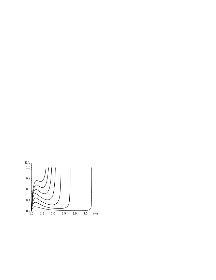
Figure 9: Wells and barriers in the scattering of two particles with the Lennard–Jones interaction potential at different impact parameters $B$.

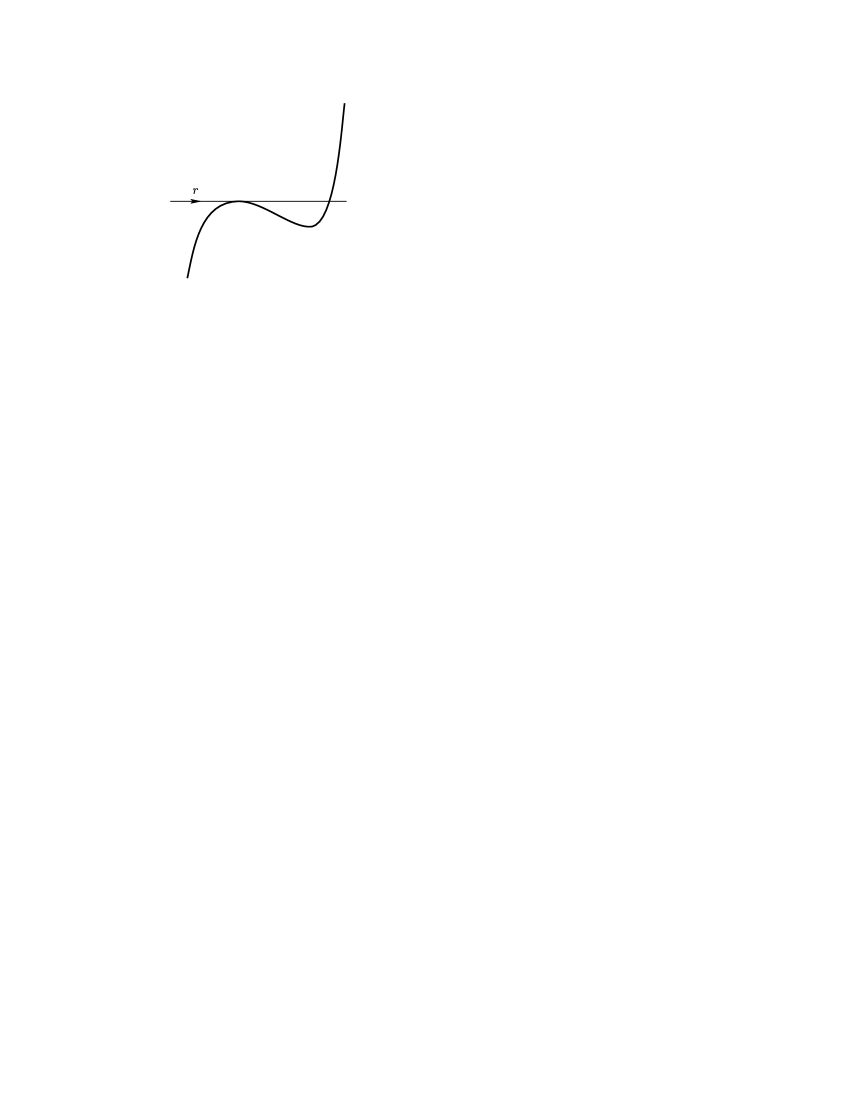
Figure 10: A trap for a fictitious particle–dimer, in the center of mass system (CMS). Here $r$ stands for the radius vector of the dimer; it is marked on the abscissa axis. A “particle” falls from the left, from the point $r=B$, where $B$ stands for the impact parameter. After reflection from the “wall”, i.e., from the potential, in the presence of viscosity, the particles meet the barrier and then after rather many reflections from the barrier and the “wall” drop on the well bottom in a greater time interval.

Let us use considerations of dimensional analysis for the scattering problem and the definition of the one-particle (the so-called thermal) attraction potential. The scattering problem is considered for the Lennard–Jones potential, and therefore there is an additional parameter of length in the problem, the parameter $a$, which is the effective radius. The attraction potential occurs in the quantum theory of the dipole–dipole interaction. If we fix the distance between the particles and assume that the semiclassical parameter $\hbar$ tends to zero, then the attractive potential vanishes. This means that, as $\hbar\to 0$, the distance between the particles decreases. It follows that the attractive potential acts between “nearest neighbors” only.

Therefore, it is natural to use the expansion of an attraction single-particle potential in powers of the radius $r$ up to $O(r^{3}/V)$ only.

The “dressed” or thermal potential $\Psi(r^{2})$ is attracting. As is well known, it was derived from the fact that the correlation sphere for the $N$-particle for the Gibbs distribution is finite [56].

One of the most interesting points of independence of a macroinstrument of a microinstrument manifests itself when applying the dimension theory [57]. A macroinstrument determines the volume $V$. According to the independence of the thermodynamic quantities on the shape of the volume $V$, the volume $V$ ensures us that we have the dimension in the dimension theory is three; however, this volume does not give us any one-dimensional measure. which is the typical length in the thermodynamic process.

A microinstrument determines the effective radius of the molecule and the mean free path. However, in dimension theory, we cannot measure the typical length of the macrothermodynamics by using the radius of the molecule or the mean free path, even if the volumeis a Torricelli tube and its typical thickness is small as compared with the case in which the vessel is a ball. These considerations show that the only possible dimensionless combination for the argument of $\Psi(r^{2})$ is

$$\Psi\Big{(}\frac{ar^{2}}{V}\Big{)}.$$

Since $a^{3}\ll V$, it follows that the expansion is

$$\Psi\Big{(}\frac{ar^{2}}{V}\Big{)}=C_{1}+C_{2}\frac{ar^{2}}{V}+O\bigg{(}\frac{a^{2}r^{4}}{V^{2}}\bigg{)}.$$ (84)

The constant $C_{1}$ gives no contribution to the scattering problem, and the thermal “single-particle” potential turns out to be proportional to the density. On the plane $\{T,\rho\}$, the maximum of the binodal (according to Fig. 8 for $T=T_{c}$) is equal with respect to $\rho$ to the very value $\rho_{c}$, which enables us to find the proportionality coefficient. It turns out to be equal to one.

The situation in which the thickness of the tube is “commensurable” to the radius of the molecule leads to quite different effects: to the superfluidity of water in a nanotube and to the freezing of water at $T^{0}=5K$ (see [58]).

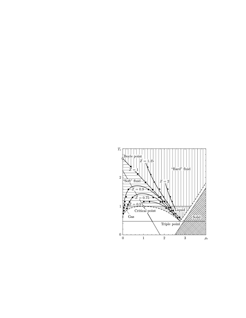
Figure 11: The $T$–$\rho$-diagram for gases corresponding to simple liquids. Here $T_{r}=T/T_{c}$ and $\rho_{r}=\rho/\rho_{c}$. The Zeno line (the straight line $Z=\frac{PV}{kNT}=1.0$) in the phase diagram. For the states $Z>1.0$ (the hard fluids), the repulsive forces dominate; for the states $Z<1.0$ (soft fluids), the attraction forces dominate.

Expanding

$$r^{2}=r^{2}_{1}+r^{2}_{2}=\frac{(r_{1}-r_{2})^{2}}{2}+\frac{(r_{1}+r_{2})^{2}}{2},$$ (85)

we can make the separation of variables in the two-particle problem to a scattering problem for a pair of particles and to the problem of their joint motion for $r_{1}+r_{2}$, just as it was done in [59]. In this case, in the scattering problem, a quadratic attraction potential (an upturned parabola) $-\rho r^{2}$ is added to the Lennard–Jones interaction potential, and $\rho=\frac{1}{V}$ for the isochoric process.

In the scattering problem thus obtained, there are two points of rest, namely, the stable one, $E_{\min}$, and the unstable point $E_{\max}$. Their ratio is a dimensionless quantity. As follows from the previous section, $Z=\frac{PV}{NT}$, where $P$ stands for the pressure, $N$ for the number of particles, $T$ for the temperature, and, due to the fact that a stable stationary point has the meaning of temperature, it follows that the ratio

$$Z=\frac{PV}{NT}=\frac{E_{\min}}{E_{\max}}$$ (86)

enables us to wrote the curves $Z=\text{const}$ in the graph $T$, $\rho=\frac{N}{V}$.

The curve at $Z=1$ is called the Zeno line (or the Bachinski parabola), and the locus of the beginnings of the curves $Z_{\max}$ (for $C_{2}\neq 0$ and $B\to\infty$) is referred to as the binodal.

Thus, in our view, the Zeno line determines the temperatures for which the dimers become practically nonexistent for a given density.

Denote by $\rho_{c}$ the value of $\rho$ at the maximal point of the binodal and denote the endpoint of this curve on the $\rho$ axis by $\rho_{B}$. In [60]. this point was referred to as the hypothetical point $\rho_{B}$ (the Boyle point).

Calculating the value of $Z_{c}$, we obtain $Z_{c}=0.296$, which coincides with the values of $Z_{c}$ for the noble gases up to thousandths. The ratio $\rho_{c}/\rho_{B}$ also coincides with the values of this quantity for the noble gases.

Table 1 shows the data corresponding to the resulting diagram (for $B=100$ in “molecular” values), and note the discrepancy between the basic dimensionless relations obtained by the data of molecular dynamics and the theoretical relations obtained by physicists from the chain BBKKI and the $N$-partial Gibbs distribution.

Table 1

$$\begin{matrix}&Z_{c}\quad&\rho_{c}/\rho_{B}\quad&T_{c}/T_{B}\\ &0.29\quad&0.273\quad&0.36\\ &0.308\quad&0.285\quad&0.38\\ &0.375\quad&0.333\quad&0.296\end{matrix}$$

On the top line of the table, the theoretical values for $Z_{c}$, $\rho_{c}/\rho_{B}$, and $T_{c}/T_{B}$, obtained using the above theory are presented. The second line contains the values of the same quantities evaluated according to the latest data of molecular dynamics and results of theoretical physicists for the Lennard–Jones potential. The third line gives the values obtained from the van der Waals equation, which is empirical.

The value of $Z_{c}$ can be computed in the experiment very accurately, and it is equal to $0.29$ for noble gases, nitrogen, oxygen, and propane. The value of $\rho_{c}/\rho_{B}$ (the ratio of the critical value of $\rho$ critical to $\rho_{B}$, i.e., to the entire length of the segment with respect to $\rho$ on which the Zeno-line “cuts” the abscissa axis away) evaluated in the above theory coincides with the corresponding values for water, argon, xenon, krypton, ethylene, and a number of other gases.

Let us present detailed calculations to find the Zeno-line.

Consider the potential

$$E(r)=\frac{-\alpha r^{4}+r^{2}U(r)}{B^{2}-r^{2}}.$$ (87)

Its first derivative is equal to

$$E^{\prime}(r)=\frac{r(2B^{2}U(r)+r(2\alpha r(-2B^{2}+r^{2})+(B^{2}-r^{2})U^{\prime}(r)))}{(B^{2}-r^{2})^{2}},$$ (88)

and the second derivative is

$$E^{\prime\prime}(R) =\frac{1}{(B^{2}-r^{2})^{3}}\bigl{(}2(B^{4}+3B^{2}r^{2})U(r)+r(-2\alpha r(6B^{4}-3B^{2}r^{2}+r^{4})$$

$$\qquad+4(B^{4}-B^{2}r^{2})U^{\prime}(r)+r^{2}(B^{2}-r^{2})^{2}U^{\prime\prime}(r))\bigr{)}.$$ (89)

We obtain a solution of the equation in the form

$$B=\sqrt{-\frac{-r^{3}U^{\prime}(r)+r^{4}U^{\prime\prime}(r)}{-8U(r)+2rU^{\prime}(r)+2r^{2}U^{\prime\prime}(r)}}.$$ (90)

Substituting the value $B(r)$ into 87, we find $E(\alpha)$, the Zeno-line, i.e., a segment, which is straight up to 3%, $T/{T_{B}}+\rho/{\rho_{B}}=1,$ where $\rho_{B}$ stands for the maximal density as $T\to 0$.

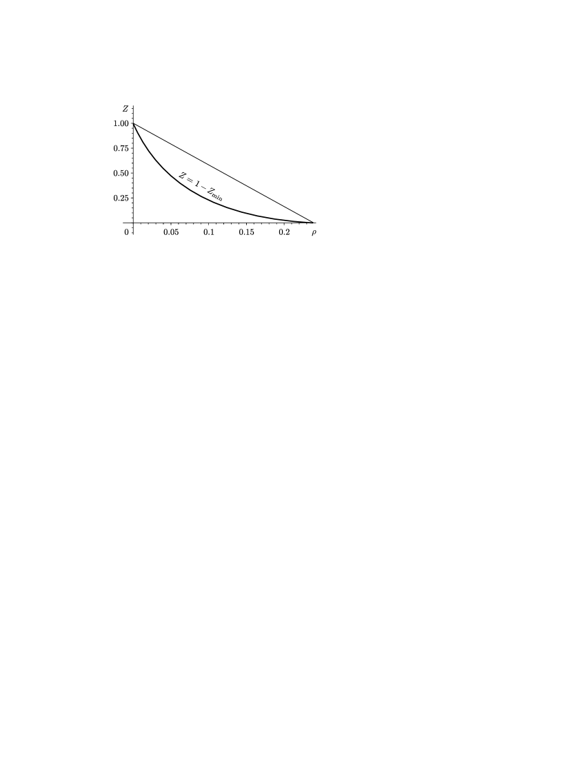
Figure 8A: Curve $1-Z_{\min}$.

4.4 Limit stretching of a liquid.
The maximum density of holes

We have $Z=P/{\rho T},$ where $\rho=\rho_{B}\left(1-T/{T_{B}}\right)$ is an isotherm-isochore. Therefore,

$$Z=\frac{P_{r}}{\rho_{B}T_{r}(1-T/T_{B})}.$$ (91)

Let us express $Z$ in terms of $\gamma$ for $Z<0$ and $\gamma<0$ and for $\mu\sim o(1/\log N)$,

$$N=A(\gamma)T_{r},\qquad P=\frac{T_{r}^{2+\gamma}\zeta(2+\gamma)}{\zeta(2+\gamma_{c})},$$

where $T_{r}=T/T_{c}$ and $P_{r}=P/P_{c}$. The value of $\rho_{B}$ is defined in this very normalization.

Therefore,

$$Z=\frac{T_{r}^{2+\gamma}\zeta(2+\gamma)}{\zeta(2+\gamma_{c})(A(\gamma)T^{2}}=\frac{T_{r}^{\gamma}\zeta(2+\gamma)}{\zeta(2+\gamma_{c})A(\gamma)}.$$ (92)

On the other hand, $N=\rho=\rho_{B}\left(1-T/{T_{B}}\right)=A(\gamma)T.$ Consequently, ${\rho_{B}}/T-{\rho_{B}}/{T_{B}}=A(\gamma)$ and

$$\left(\frac{1}{T}\right)^{|\gamma|}=\left(\frac{1}{\rho_{B}}A(\gamma)+\frac{1}{T_{B}}\right)^{|\gamma|}.$$

Substituting this into 92, we obtain

$$Z=\frac{\zeta(\gamma+2)}{\zeta(\gamma_{c}+2)}\frac{\left(\dfrac{1}{\rho_{B}}A(\gamma)+\dfrac{1}{T_{B}}\right)^{|\gamma|}}{A(\gamma)},$$

and $A(\gamma)\to\infty$ as $\gamma\to-1$.

Therefore, as $\gamma\to-1$, the value $1/T_{B}$ is negligible. Consequently,

$$Z|_{\gamma\to-1}\simeq\frac{\zeta(\gamma+2)}{\rho_{B}^{|\gamma|}\zeta(\gamma_{c}+2)A(\gamma)^{1-|\gamma|}}.$$ (93)

Here $\gamma_{c}$ corresponds to $Z_{c}$, which is the minimal value of $Z$ on the critical isotherm for $P=1$ (see Fig, 9).

Since

$$A(\gamma,\Lambda)=(\Lambda^{\gamma_{c}-\gamma}c(\gamma))^{1/1+\gamma},$$

where $\gamma<0$, it follows that

$$A(\gamma,\Lambda)^{1+\gamma}=\Lambda^{\gamma_{c}-\gamma}c(\gamma),$$

where

$$c(\gamma)=\left[\int_{0}^{\infty}t^{\gamma}\,dt\left(\frac{1}{t}-\frac{1}{e^{t}-1}\right)\right].$$

Hence,

$$Z|_{\gamma\to-1}=\frac{\zeta(2+\gamma)}{\rho_{B}^{|\gamma|}\zeta(2+\gamma_{c})c(\gamma)\Lambda^{\gamma_{c}+1}}.$$

The expression $c(\gamma)$ tends as $\gamma\to-1$ to $(1/2)\log\varepsilon$, where $\varepsilon$ stands for the lower limit of the integral expression for $A(\gamma)^{1-|\gamma|}$ at $\gamma=-1$.

Similarly, the expression $\zeta(\gamma+2)$ at $\gamma=-1$ is equal to $\log\varepsilon$.

Hence

$$Z|_{\gamma\to-1}=\frac{2}{\rho_{B}\zeta(\gamma_{c}+2)\Lambda^{\gamma_{c}+1}}$$

as $\gamma\to 0$ and $Z\to 0$. Therefore,

$$Z<Z_{\max}<\text{const}$$

for all values of $\gamma$.

Hence, by 91,

$$P_{r}=Z\rho_{B}T_{r}\left(1-\frac{T_{r}}{T_{B}}\right)\leq Z_{\max}\frac{T_{B}}{2}.$$ (94)

Moreover, it is clear that $P_{r}\to 0$ as $T_{r}\to 0$ and $\gamma\to 0$.

The value of $\lambda$ determines the minimum of $P_{r}$ and the maximal density of holes.

To determine the gas-liquid transition, as in Sec. 2.3, with the correction to the Zeno line taken into account, we derive equations of the form 25-26, by normalized the activity for the critical isotherm.

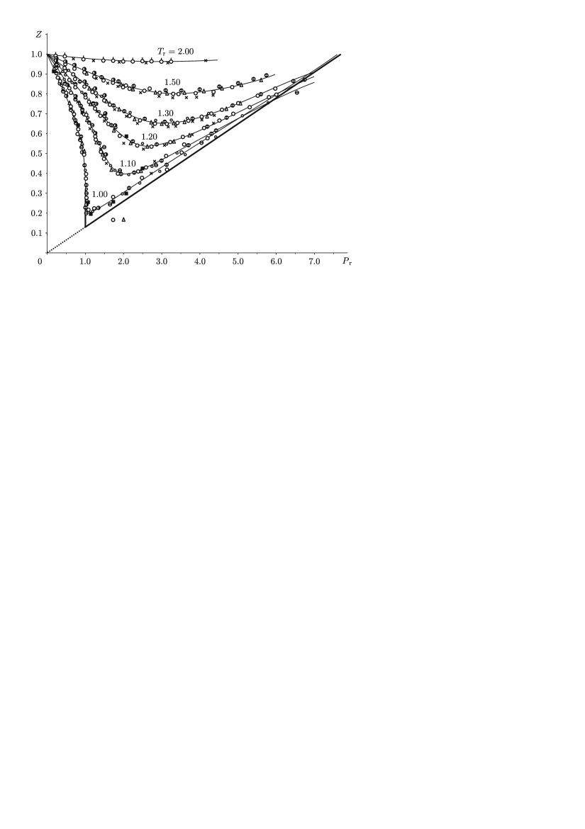
Figure 9: The picture of the law of corresponding states for molecules of different gases. Thin lines show isotherms for methane. Different symbols on isotherms correspond to argon, carbon dioxide, water, etc. The fact that isotherms of different gases are close to one another illustrates the empirical law of corresponding states. The theoretical isotherm (the solid line) does not fully coincide with the experimental one. This is an effect of the same type as the jump of the critical exponents. The viscosity (the Wiener quantization) smooths the sharp angle of the limit isotherm (as $\varepsilon\to 0$).

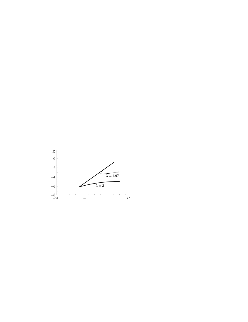
Figure 10: Spinodal curves in the domain $P<0$. The inclined line is the continuation of the theoretical critical isotherm shown in Fig. 9 to the domain of negative values of $P$ and $Z$. The initial point of the curve $\Lambda=1/3$ ($\lambda=1/\Lambda$) is at a distance from the point $P=0$, and the starting point $\Lambda=0.5086$ ($\lambda=1/\Lambda=1.97$) of the curve coincides with the point of intersection of the dashed line and the solid line.

4.5 A coarser measuring instrument
and the law of corresponding states

Obviously, the rougher is the device, the greater is the dissipation parameter, and therefore the more important is the uncertainty principle. If our device does not distinguish some molecules from one another, then this is a rough instrument. It is not necessary that the device itself be so rough. It is sufficient to say that the experimenter does not want to distinguish molecules and computes the density roughly, counting all the molecules for which he wants to construct a “rough” thermodynamics. Hence, when speaking more precisely, from the point of view of mathematics, the rougher thermodynamics we want to receive, the more rough will be the answer due to the Wiener uncertainty principle.

Our rough instrument does not distinguish particles not only in mixtures. Measuring different particles, the observer thinks that these are the same molecules, and only the measurements are somewhat scattered. This is even a more rough thermodynamics. It is referred to the fluid part, when the gas-liquid is not distinguished, clusters occur, etc. The critical points are on the boundary of the fluid domain, and we approach them from the side of the fluid domain for $T\geq T_{c}$.

When considering above the phase transition, we have equated the chemical potentials of the liquid and the gas phases on the critical isotherm, assuming that there is no phase transition there. We considered the case in which the viscosity vanishes, and we obtained a phase transition which was not smeared. Now, when considering the problem with a coarser device, we no longer have any right to assume that the dissipation tends to zero. The uncertainty principle gives us a fairly large smearing of the phase transition; however, it happens on a “rough” critical isotherm which is measured by a rough instrument. The latter cannot distinguish now not only particles of a single pure gas but does not distinguish particles of different gases either.

We have compared the Wiener quantization of thermodynamics with the dissipation resulting in a shock wave. However, the dissipation may be different in different substances, while we are interested now in the Hugoniot conditions for the entire mixture, and we do not want to distinguish stratificationally occurring internal shock waves within a common shock wave. This is particularly evident when the dissipative parameters of viscosity and thermal conductivity are different (see [62], § 95), the viscosity $\nu$ is small, and the thermal conductivity is relatively large, $\chi\gg\nu$. If the processes inside the shock wave are not of interest for us, then we pose the Hugoniot conditions on a shock wave spread with respect to heat conductivity.

On the other hand, if the values of viscosity in a mixture of different gases are different but not dramatically different from one another, then the width of a shock wave thus obtained is defined by the average viscosity.

Since, as a rule, the Bose–Einstein-type distribution is considered in the three-dimensional case, it would seem to be natural to add the integration over the coordinates to the integration of the momenta. Then the three-dimensional volume $V$ would occur as if this is a natural way. It would seem that there can be a generalization if the dimension of volume is changed when changing the dimension of the momenta. However, in the manual [2], when considering a photon gas, the integration of the Hamiltonian of the oscillator is carried out both over the momenta and over the coordinates, and, nevertheless, the three-dimensional volume $V$ is taken as the multiplier for the distribution.

Note first that number theory gives, for dimension two, a distribution without the volume $V$ (see Example 1), as well as the initial relations in [2] both for the Boltzmann–Maxwell ideal gas and for the Bose–Einstein ideal gas (see 1–4). Further, in [2], both the distribution for bosons and the distribution for photons are multiplied by the three-dimensional volume $V$. Certainly, the main distribution is the distribution without the volume $V$, and its multiplication by $V$ is caused by the correspondence with thermodynamics in which the pair ‘the volume $V$ – the pressure $P$’ is the most important tool.

Therefore, the most natural generalization to the nonideal distribution is the multiplication of a fractional Bose distribution by a function of $V$ of the form $V\varphi(V/V_{0})$, where $V_{0}$ stands for some reference volume and the function $\varphi(x)$ is smooth.

The introduction of this multiplier does not change the distribution caused by number theory [63] in which the variable $V$ is eliminated by the change of the variable $N/V=\rho$. However, if we consider $V\varphi(V/V_{0})$ as a multiplier, where $V_{0}$ is some typical volume, then the relation for the three-dimensional Lagrangian manifold $\Lambda^{3}$ in the six-dimensional phase space $\{P,V;T,S;\mu,N\}$ is preserved, whereas the variables $V$ and $N$ do not convert here into a single variable $\rho=N/V$. Therefore, the volume and the number of particles are changed on the isochore $\rho=\text{const}$ in general. This modification of the $\Omega$-potential does not change the specific entropy, which is also of importance.

In a mixture of gases, we are to choose a reference gas in which the difference between the vapor and the liquid is the lowest possible, for example, from the point of view of the number of dimers. This gas is the mercury vapor ($Z_{c}=0.4$). Let us carry out a normalization of activity 26 for an isotherm of this gas at $Z=0.4$ and assume that there is no phase transition on the critical isotherm of mercury. In accordance with what was said above, the rough device cannot distinguish among molecules of $l$ distinct gases. Let us calculate the average degree of freedom for these molecules by taking the arithmetic mean of the values of the entropy of $l$ pure gases (see 13) on the basis of experimental data for $Z_{c}^{i}$, $i=1$, $2$, …, $l$, pure gases (see 13),

$$(\gamma_{average}+2)\frac{\zeta(\gamma_{average}+2)}{\zeta(\gamma_{average}+1)}=Z_{average}(\gamma_{average}+2)=\frac{1}{l}\sum_{i=1}^{l}(\gamma_{i}+2)\frac{\zeta(\gamma_{i}+2)}{\zeta(\gamma_{i}+1)}.$$

The highest value $Z_{c}=0.4$ is given by mercury (Hg), and therefore the average number of degrees of freedom of this family of molecules is certainly less, and therefore $Z_{average}<Z_{c}$ (mercury), $\gamma<\gamma_{Hg}$. The critical pressure is greater than that for mercury, $\zeta(\gamma_{Hg}+2)<\zeta(\gamma_{average}+2)$.. Therefore, the value we have chosen for mercury, $P_{r}=1$, is less than $P_{average}=\zeta(\gamma_{average}+2)/\zeta(\gamma_{Hg}+2)$. Thus, the value $P_{r}=1$ for $Z_{Hg}$ belongs to the domain of the phase transition “gas-liquid” for $Z_{average}$. This implies that, for $P_{r}=1$, the phase transition to liquid occurs at $Z_{average}$.

This phase transition to liquid can be seen in Fig. 9, in the form a vertical bounded by a black sloping line depicting the liquid.

Taking into account the Zeno line influences the form of the $\Omega$-potential as follows:

$$\Omega(\mu,T)=-\Lambda^{\gamma+1}V\varphi(V/V_{0})\frac{T^{\gamma+2}}{\Gamma(\gamma+2)}\int_{0}^{\infty}\frac{t^{\gamma+1}\,dt}{(e^{t}/y)-1}=-\Lambda^{\gamma+1}T^{\gamma+2}V\varphi(V/V_{0})\operatorname{Li}_{\gamma+2}(y),$$ (95)

where $y=\exp(\mu/T)$ is the activity and $\mu$ stands for the chemical potential.

Let us write out the differential equations for $\varphi(x)$ with regard to the relations on the Zeno line,

$$T_{z}=T_{B}\left(1-{\rho_{z}}/{\rho_{B}}\right),\qquad P_{z}=\rho_{z}T_{B}\left(1-{\rho_{z}}/{\rho_{B}}\right),$$ (96)

where the subscript $z$ means that the corresponding values are taken on the Zeno line, i.e., for $Z=1$.

Let us construct the relation $Z=1$ on the Zeno line. This relation is of the form

$$Z=\frac{\partial\Omega/\partial V}{T_{z}\partial\Omega/\partial\mu}=\frac{\varphi(V_{z}/V_{0})+(V_{z}/V_{0})\varphi^{\prime}(V_{z}/V_{0})}{\varphi(V_{z}/V_{0})}\cdot\frac{\operatorname{Li}_{\gamma+2}(y_{z})}{\operatorname{Li}_{\gamma+1}(y_{z})}=1.$$ (97)

It follows from 96 on the Zeno line that

$$T_{z}^{2+\gamma}[\varphi(V_{z}/V_{0})+(V_{z}/V_{0})\varphi^{\prime}(V_{z}/V_{0})]\operatorname{Li}_{\gamma+2}(y_{z})=\left(N/{V_{z}}\right)T_{B}\left(1-N/({V_{z}\rho_{B}})\right).$$ (98)

Assume that the conditions $N/V=\text{const}$ and $N=\text{const}$ hold on the isochore and on the Zeno line defined by relation 96. It follows from 97 and 98 that

$$T_{B}^{\gamma+1}\left(1-N/({V_{z}\rho_{B}})\right)^{\gamma+1}\varphi(V_{z}/V_{0})\operatorname{Li}_{\gamma+1}(y_{z})=N/({V_{z}\rho_{B}}).$$ (99)

Here $N/V_{z}=\text{const}$ and $N=\text{const}$, and hence this equation contains unknowns $y_{z}$, $V_{z}$, and $\varphi(V_{z}/V_{0})$.

After finding the value $y_{z}$ as a function of $V_{z}$ and $\varphi(V_{z}/V_{0})$, we substitute it into formula 97, thus transforming equation 97 into a differential equation for the function $\varphi(x)$ depending on the constants $\rho_{B}$ and $T_{B}$. The equation for $\varphi(V)$ enables one to find the point $y_{z}(\rho)$ on the Zeno line, and, after this, the isochore is changed only at the expense of the modification of activity $a=e^{-\mu/T}$ from $y_{z}(\rho)$ to $a=1$ for the polylogarithm $\operatorname{Li}_{\gamma+1}(a)$. The function $\varphi(V)$ is not reflected in the structure of the isochore, and it is reflected in scaling only (see Fig. 11).

The most important problem in the theory of differential equations, the existence problem for a solution, remains open. Physicists pay less attention to this problem than mathematicians.

What are conditions for the existence of a solution of equations 97–98?

Introduce the notation $T_{s}=T_{\text{standard}}=T/T_{m}$ and $P_{s}=P_{\text{standard}}=P/P_{m}$, where $T_{m}$ and $P_{m}$ are defined by the formulas

$$P_{m}=T_{m}^{\gamma+2},\qquad V_{0}=V_{m}=V_{\max},$$

and $Z_{m}=Z_{\max}$ and $\rho_{m}=\rho_{\min}$ are defined below.

Since $N_{c}$ does not depend on $T$, it follows that $V$ and $N$ are constant along the isochore $V=V_{m}$.

Let us write out the above relations at the point $T_{s}=1$, $P_{s}=1$:

$$[\varphi(V_{z}/V_{0})+(V_{z}/V_{0})\varphi^{\prime}(V_{z}/V_{0})]\zeta(\gamma+2)=1,\qquad V_{m}\varphi(1)\zeta(\gamma+1)=N_{c},\qquad V_{m}=V_{\max},$$ (100)

Hence,

$$Z_{m}=\frac{V_{m}}{N_{c}}\frac{\zeta(\gamma+1)}{\zeta(\gamma+2)}\cdot\frac{\operatorname{Li}_{\gamma+2}(1)}{\operatorname{Li}_{\gamma+1}(1)}=\frac{V_{m}}{N_{c}}=\frac{1}{\rho_{m}}.$$ (101)

Since we construct isochores $V=\text{const}$ on the plane $\{Z,P\}$, it follows that $V_{m}=V_{z}$. Eliminating $(V_{z}\varphi(V_{z}/V_{0})^{\prime}$ from 100 by using 99, we obtain

$$T_{B}^{\gamma+1}\left(1-\frac{1}{Z_{m}\rho_{B}}\right)^{\gamma+1}\frac{1}{\zeta(\gamma+2)}\operatorname{Li}_{\gamma+2}(y_{z})=\frac{1}{Z_{m}}.$$ (102)

Since $V_{m}=V_{z}$, we see that

$$\varphi(1)=N_{c}(\zeta(\gamma+1)V_{m})^{-1},\qquad\varphi(1)+\varphi^{\prime}(1)=(\zeta(\gamma+2))^{-1},$$ (103)

and it follows from 97 on the Zeno line that the following equation holds:

$$\frac{\operatorname{Li}_{\gamma+2}(y_{z})}{\operatorname{Li}_{\gamma+1}(y_{z})}\cdot\frac{V_{m}}{N_{c}}\cdot\frac{\zeta(\gamma+1)}{\zeta(\gamma+2)}=1.$$ (104)

Eliminating $y_{z}$, we find a relation for $Z_{m}$ and $\gamma$. The maximum value of $Z_{m}$ depends on the values of $\rho_{B}$ and $T_{B}$ only. For mercury, this maximum is obtained for $\gamma_{m}=\gamma_{\min}=0.1$, and $Z_{m}=0.4$, which coincides with the value of $Z_{c}$ for mercury. This coincidence, which depends on $\rho_{B}$ and $T_{B}$, holds for mercury Hg only (among all the elements of the periodic table), which confirms the correct choice of the $\Omega$-potential 95.

The family of isochores, according to system 98–99 with the above initial condition 103, is shown in Fig. 11.

The first relation for the limit isochore $V_{m}/N_{c}=Z_{m}$, for $\gamma=\gamma_{m}$, is of the form

$$Z=Z_{m}\cdot\frac{\zeta(\gamma+1)}{\zeta(\gamma+2)}\cdot\frac{\operatorname{Li}_{\gamma+2}(y)}{\operatorname{Li}_{\gamma+1}(y)},\qquad 1\leq y\leq y_{z}(\gamma).$$ (105)

Since $P_{s}=T_{s}^{\gamma+2}\operatorname{Li}_{\gamma+2}(y)/\zeta(\gamma+2)$ and $N=T_{s}^{\gamma+1}\operatorname{Li}_{\gamma+1}(y)V_{m}$, it follows that the other relation is

$$P_{s}=\left(\frac{\zeta(\gamma+1)}{\operatorname{Li}_{\gamma+1}(y)}\right)^{(\gamma+2)/(\gamma+1)}\frac{\operatorname{Li}_{\gamma+2}(y)}{\zeta(\gamma+2)},\qquad 1\leq y\leq y_{z}(\gamma).$$ (106)

Equations 105 and 106 give an almost straight segment of the isochore.

Starting from $Z<0.4$ (for example, for a van der Waals gas), the phase transition to a liquid occurs for indistinguishable particles of the law of corresponding states. This gives a broad area (at the expense of the uncertainty principle of a “rough device”) around the line segment $P=1$, $T_{s}=1$, $Z<0.4$.

Remark 5. Since the rightmost isochore (which is not shown in Fig. 11) is a segment of a straight line, it follows that all isochores of high density must also be line segments. They pass through the point $\rho>\rho_{m}$ on the Zeno line and the point $Z_{0}=1/\rho$ on the line $P_{s}=1$. We thus obtain (when including the isochores shown in Fig. 11) a complete family of isochores for $Z\leq 1$, $P\geq 1$, related to the law of corresponding states. To any point of an isochore in the plane $\{Z,P\}$ there corresponds a point of temperature, and we construct isotherms which, up to the Wiener uncertainty principle, correspond to the experimental law of corresponding states (Fig. 12).

In Fig. 13, the graph of an experimental isotherm for mercury is presented; this graph was kindly evaluated by Professor V. S. Vorob’ev, according to the most recent data, at the instance of me. Note that the passage gas–liquid happens at $T=1473\,K$ along a slanting line rather than a vertical one, which is related to nonzero viscosity and the Wiener uncertainty principle. This effect is of the same nature as the jump of critical exponents and “thickness of the layer” of a shock wave.

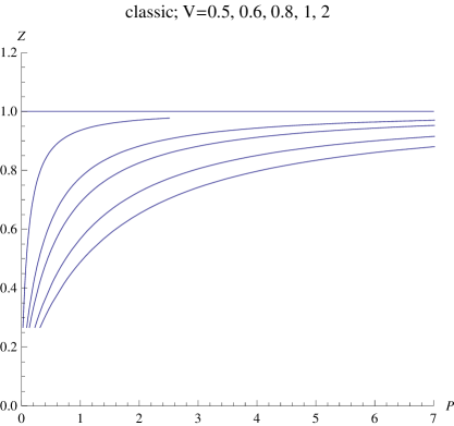
Figure 11: The graph for the isochore of the polylogarithm $\operatorname{Li}_{\gamma+1}(a)$ for $\gamma=2$.

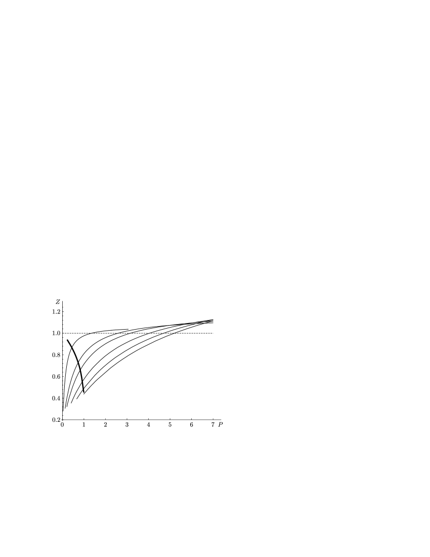
Figure 12: The dotted line shows the Zeno line $Z=1$. The bold line is the critical isotherm of a real gas (mercury) which is calculated theoretically, and the fine lines are isochores of mercury for $T<T_{\text{c}}$.

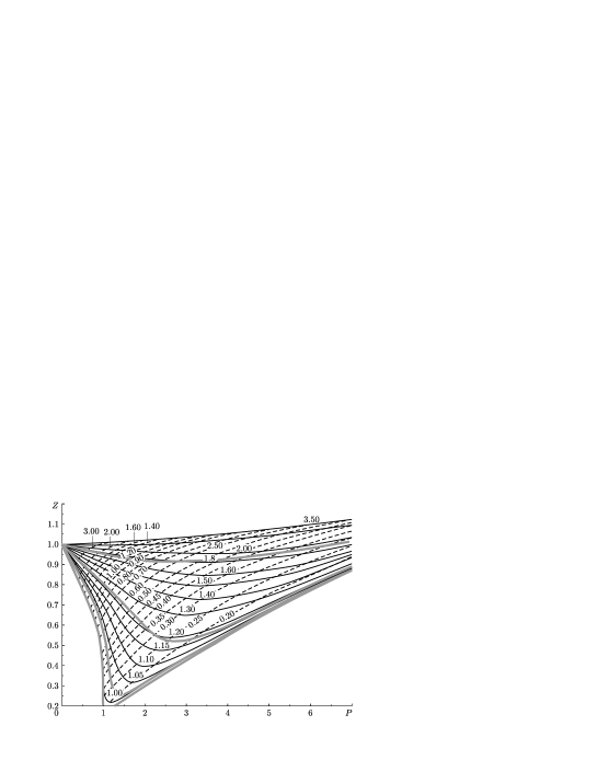
Figure 13: The thin solid lines represent the experimental isotherms for methane (see Fig. 9). The dotted lines approximating the experimental curves are based on theoretical data. The dashed curves show the experimental isochores.

The  author  is  grateful  to  V. V. Brazhkin, A. E. Gekhman, B. V. Egorov, D. Yu. Ivanov, Yu. M. Kagan, A. G. Kulikovskii, G. A. Martynov, I. V. Melekhov, D. S. Minenkov, V. N. Ryzhov, A. S. Kholevo, and A. V. Chaplik for fruitful discussions. The author is especially indebted to Professor V. S. Vorob’ev who had verified all graphs and and carried out an entire series of the most important comparisons of theoretical results with experimental data.

References

- [1] L. D. Landau and E. M. Lifshits, Course of Theoretical Physics, Vol. 3: Quantum Mechanics: Non-Relativistic Theory, 2nd ed. (Nauka, Moscow, 1964; transl. of the 1st ed., Pergamon Press, London–Paris and Addison-Wesley Publishing Co., Inc., Reading, Mass., 1958).
- [2] L. D. Landau and E. M. Lifshits, Course of theoretical physics. Vol. 5: Statistical physics (Nauka, Moscow, 1964; Pergamon Press, Oxford–Edinburgh–New York, 1968).
- [3] E. M. Apfelbaum and V. S. Vorob’ev, “Correspondence between the ideal Bose gas in a space of fractional dimension and a dense nonideal gas according to Maslov scheme”, Russ. J. Math. Phys. 18 (1), 19–25 (2011).
- [4] A. N. Shiryaev, Probability, Vol. 1: Elementary Probability Theory. Mathematical Foundations. Limit Theorems (MCCME, Moscow, 2004) [in Russian].
- [5] V. P. Maslov and T. V. Maslova, “Unbounded probability theory and its applications,” Teor. Veroyatnost. i Primenen. 57 (3), 471–498 (2012) [in Russian].
- [6] P. Erdős and J. Lehner, “The Distribution of the Number of Summands in the Partitions of a Positive Integer,” Duke Math. J. 8 (2), 335–345 (June 1941).
- [7] V. P. Maslov, “Unbounded Probability Theory Compatible with the Probability Theory of Numbers,” Math. Notes, 91 (5) 603–609, (2012).
- [8] N. N. Bogolyubov, Selected works in three volumes, Vol. 3 (Izdat. “Naukova Dumka”, Kiev, 1971) [in Russian].
- [9] V. P. Maslov, “The Boundary of a Volume as a Trap Ensuring the Phase Transition in an Ideal Gas,” Math. Notes, 92 (5) 657–664, (2012).
- [10] V. P. Maslov, “The Effect of a Natural Trap (the Boundary of the Volume) on the Bose Distribution of Quantum Particles in the Three-Dimensional and Two-Dimensional Cases,” Math. Notes, 92 (6) 868–871, (2012).
- [11] V. P. Maslov, “Ideal Gas/Liquid Transition as a Generalization of the Problem of ‘partitio numerorum’ ”, Russ. J. Math. Phys. 19 (4) 486–500, (2012).
- [12] V. P. Maslov, “The effect of measuring instrument in the “Bose condensate” of classical gas, in the phase transition, and in experiments with negative pressure,” Teoret. Mat. Fiz., 2013 (in print).
- [13] V. E. Nazaikinskii, “On the Asymptotics of the Number of States for the Bose–Maslov Gas,” Math. Notes, 91 (6) 816–823, (2012).
- [14] V. E. Nazaikinskii, “On the Entropy of the Bose–Maslov Gas,” Dokl. Ross. Akad. Nauk, 448 (3), 1–3 (2013) [in Russian].
- [15] V. P. Maslov, Threshold Levels in Economics, arXiv:0903.4783v2 [q-fin.ST], 3 Apr 2009.
- [16] V. P. Maslov and P. P. Mosolov, Nonlinear Wave Equations Perturbed by Viscous Term. De Gruyter Expositions in Mathematics 31 ( Walter de Gruyter, Berlin–New York, 2000).
- [17] V. P. Maslov, Quantum Economics (Nauka, Moscow, 2006) [in Russian].
- [18] V. P. Maslov and P. P. Mosolov, “Asymptotic behavior as of trajectories of point masses, interacting according to Newton’s gravitation law,” Izv. Akad. Nauk SSSR Ser. Mat. 42 (5), 1063–1100 (1978) [Math. USSR-Izv. 42 (5), 1101–1119 (1978) (1979)].
- [19] V. P. Maslov and A. S. Mishchenko, “Geometry of a Lagrangian Manifold in Thermodynamics,” Russ. J. Math. Phys. 10 (2), 161–172 (2003).
- [20] N. E. Hurt, Geometric Quantization in Action (D. Reidel Publishing Co., Dordrecht–Boston, Mass., 1983; Mir, Moscow, 1985).
- [21] V. P. Maslov, Asymptotic Methods and Perturbation Theory (Nauka, Moscow, 1988) [in Russian].
- [22] R. P. Feynman and A. Hibbs, Quantum Mechanics and Path Integrals (McGraw-Hill, New York, 1965; Mir, Moscow, 1968).
- [23] V. P. Maslov, “Nonstandard Characteristics in Asymptotic Problems,” Uspekhi Mat. Nauk, 38 (6), 3–36 (1983) [Russian Math. Surveys 38 (6), 1–42 (1983)].
- [24] G. L. Litvinov, Maslov dequantization, idempotent and tropical mathematics: a brief introduction, J. Math. Sci. 140 (3), 426–444 (2007).
- [25] V. P. Maslov, “Critical Indices as a Consequence of Wiener Quantization of Thermodynamics,” Theoret. Mat. Fiz. 170 (3), 458–470 (2012) [Theoret. and Math. Phys. 170 (3), 384–393 (2012)].
- [26] V. P. Maslov, Perturbation theory and asymptotic methods (Izdat. Moskov. Univ., Moscow, 1965) [in Russian].
- [27] V. P. Maslov, Quantization of Thermodynamics and Ultrasecond Quantization (Inst. Kompyuternykh Issledovanii, Moscow, 2001) [in Russian].
- [28] V. P. Maslov, “A model of classical thermodynamics based on the partition theory of integers, Earth gravitation and semiclassical asymptotics. I,” Russian J. Math. Phys. 24 (3), 354–372 (2017).
- [29] V. P. Maslov, “A model of classical thermodynamics and mesoscopic physics based on the notion of hidden parameter, Earth gravitation, and semiclassical asymptotics. II,” Russian J. Math. Phys. 24 (4), 494–504 (2017).
- [30] V. P. Maslov, Complex Markov Chains and the Feynman Path Integral for Nonlinear Equations (Nauka, Moscow, 1976) [in Russian].
- [31] V. P. Maslov, “Quasithermodynamic correction to the Stefan–Boltzmann law,” Teoret. Mat. Fiz. 154 (1), 207–208 (2008) [Theoret. and Math. Phys. 154 (1), 175–176 (2008)].
- [32] W.-S. Dai, M. Xie, “Gentile statistics with a large maximum occupation number,” Annals of Physics 309, 295–305 (2004).
- [33] V. P. Maslov, “New approach to classical thermodynamics,” Math. Notes 100 (1–2) 154–185 (2016).
- [34] V. P. Maslov and V. E. Nazaikinskii, “Conjugate variables in analytic number theory. Phase space and Lagrangian manifolds,” Math. Notes 100 (3–4), 421–428 (2016).
- [35] V. P. Maslov, S. Yu. Dobrokhotov, and V. E. Nazaikinskii, “Volume and entropy in abstract analytic number theory and thermodynamics,” Math. Notes 100 (5–6), 828–834 (2016).
- [36] V. P. Maslov, “New insight into the partition theory of integers related to problems of thermodynamics and mesoscopic physics,” Math. Notes 102 (1–2) 234–251 (2017).
- [37] V. P. Maslov, “On the hidden parameter in quantum and classical mechanics,” Math. Notes 102 (5–6), 890–893 (2017).
- [38] A. G. Postnikov, Introduction to Analytic Number Theory (Nauka, Moscow, 1971).
- [39] V. P. Maslov, “Two first principles of Earth surface thermodynamics. mesoscopy, energy accumulation, and the branch point in boson–fermion transition*,” Math. Notes 102 (6), 824–835 (2017).
- [40] V. P. Maslov, “Mathematical Aspects of Weakly Nonideal Bose and Fermi Gases on a Crystal Base”, Functional Anal. Appl. 37 (2), 94–102 (2003).
- [41] de L. Broglie, “Wave mechanics and the atomic structure of matter and radiation,” J. Phys. Radium 8 (5), 225–241 (1927).
- [42] J. S.Bell, “ On the Einstein Podolsky Rosen paradox,” Physics 1 (3), 198–200 (1964).
- [43] N. Bohr, F. Kalckar “On the transformation of atomic nuclei due to collisions with material particles. General theoretical remarks,”. Kgl. Danske Vid. Selskab. Math. Phys. Medd. 14 (3), (1937).
- [44] V.P Maslov, “Probability Distribution for a Hard Liquid,” Math. Notes, 97 (6) 909–918 (2015).
- [45] Maslov, V. P. Locally ideal liquid. Russian J. Math. Phys., 22 (3), 361–373 (2015).
- [46] V. P. Maslov, “Analytical number theory and the energy of transition of the Bose gas to the Fermi gas. Critical lines as boundaries of the noninteracting gas (an analog of the Bose gas) in classical thermodynamics,” Russian J. Math. Phys., 25 (2), 220–232 (2018).
- [47] A. Robinson, Non-standard analysis (North-Holland Publishing Co., Amsterdam, 1966).
- [48] V.V. Kanovei, M. Reeken, Nonstandard Analysis, Axiomatically (Springer, 2004).
- [49] E. V. Shchepin, “The Leibniz differential and the Perron–Stieltjes integral,” J. Math. Sci. 233 (1), 157–171 (2018).
- [50] V. P. Maslov, “Solution of the Gibbs paradox in the framework of classical mechanics (statistical physics) and crystallization of the gas C60,” Mat. Zametki 83 (5), 787–791 (2008) [Math. Notes 83 (5–6), 716–722 (2008)].
- [51] V. P. Maslov and O. Yu. Shvedov, The Complex Germ Method in Many-Particle Problems and in Quantum Field Theory (Editorial URSS, Moscow, 2000) [in Russian].
- [52] M. Schönberg, “Application of second quantization methods to the classical statistical mechanics,” Nuovo cimento 9 (12), 1139-1182 (1952); “Application of second quantization methods to the classical statistical mechanics (II),” Nuovo cimento 10 (4), 419–472 (1953).
- [53] V. P. Maslov, “New look on the thermodynamics of gas and at the clusterizaton,” Russ. J. Math. Phys. 15 (4), 494–511 (2008).
- [54] V. P. Maslov and G. V. Koval’, “On a generalization of the Bardeen–Cooper–Schrieffer method for pairwise interactions,” Teoret. Mat. Fiz. 154 (3), 584–592 (2008) [Theoret. and Math. Phys. 154 (3), 495–502 (2008)].
- [55] E. M. Apfelbaum and V. S. Vorob’ev, “Correspondence between the critical and the Zeno-line parameters for classical and quantum liquids”, J. Phys. Chem. B 113, 3521–3526 (2009).
- [56] G. A. Martynov, Classical Statistical Physics. Theory of Liquids (Intellekt, Moscow, 2011).
- [57] L. I. Sedov, Similarity and dimensional methods in mechanics (Nauka, Moscow, 1977; transl. of the 1st ed. Academic Press, New York–London, 1959).
- [58] V. P. Maslov, “Dependence of the superfluidity criterion on the capillary radius,” Teoret. Mat. Fiz. 143 (3), 307–327 (2005) [Theoret. and Math. Phys. 143 (3), 741–759 (2005)].
- [59] V. P. Maslov, “Thermodynamics of fluids: The law of redestribution of energy, two-dimensional condensate, and -mapping,” Teoret. Mat. Fiz. 161 (3), 422–456 2009) [Theoret. and Math. Phys. 161 (3), 1681–1713 (2009)].
- [60] E. M. Apfelbaum, V. S. Vorob’ev, and G. A. Martynov, “Triangle of Liquid-Gas States”, J. Phys. Chem. B, 110, 8474–8480 (2006).
- [61] L. I. Mandelshtam and M. A. Leontovich, “To the theory of the absorption of sound in liquids,” Zh. Eksp. Teor. Fiz. [Sov. Phys. JETP] 7 (3), 438–449 (1937).
- [62] L. D. Landau and E. M. Lifshits, Theoretical Physics, Vol. VI, Hydrodynamics (Nauka, Moscow, 1986).
- [63] A. M. Vershik, “Statistical mechanics of combinatorial partitions, and their limit shapes,” Functional. Anal. i Prilozhen. 30 (2), 19–39 (1996) [Functional Anal. Appl. 30 (2), 90–105 (1996)].
- [64] V. P. Maslov and V. E. Nazaikinskii, “On the distribution of integer random variables related by a certain linear inequality: I,” Mat. Zametki 83 (2), 232–263 (2008) [Math. Notes 83 (2), 211–237 (2008)].
- [65] V. P. Maslov and V. E. Nazaikinskii, “On the distribution of integer random variables related by a certain linear inequality: II,” Mat. Zametki 83 (3), 381–401 (2008) [Math. Notes 83 (3), 345–363 (2008)].
- [66] A. I. Anselm, Foundations of Statistical Physics and Thermodynamics (Nauka, Moscow, 1973).
- [67] H. Eyring, Basic Chemical Kinetics (Wiley, New York, 1980; Mir, Moscow, 1985).
- [68] V. P. Maslov, “Bose-condensate in the two-dimensional case, the -point, and the Thiess-Landau two-fluid model,” Teoret. Mat. Fiz. 159 (3) 174–176, (2009); “Taking parastatistical corrections to the Bose-Einstein distribution into account in the quantum and classical cases,” Teoret. Mat. Fiz. 172 (3) 468–478, (2012) [Theoret. and Math. Phys.].
- [69] V. P. Maslov, Operator Methods (Nauka, Moscow, 1973).
- [70] V. P. Maslov, Bose Condensate in the D-Dimensional Case, in Particular, for , arXiv:1207.0019v2 [cond-mat.quant-gas], 3 July 2012.
- [71] P. Erdős, “On some asymptotic formulas in the theory of partitions,” Bull. Amer. Math. Soc. 52, 185–188 (1946).