On the electron to proton mass ratio and the proton structure

Abstract

We derive an expression for the electron to nucleon mass ratio from a reinterpreted lattice gauge theory Hamiltonian to describe interior baryon dynamics. We use the classical electron radius as our fundamental length scale. Based on expansions on trigonometric Slater determinants for a neutral state a specific numerical result is found to be less than three percent off the experimental value for the neutron. Via the exterior derivative on the Lie group configuration space u(3) we derive approximate parameter free parton distribution functions that compare rather well with those for the $u$ and $d$ valence quarks of the proton.

short title: Baryon phenomena I

1 The mass ratio and the model

The ratio we get between the electron mass $m_{e}$ and the proton mass $m_{p}$ is

$$\frac{m_{e}}{m_{p}}=\frac{\alpha}{\pi}\frac{1}{\rm{E}},$$ (1)

where $\alpha=e^{2}/(4\pi\epsilon_{0}\hbar c)$ is the fine structure constant (Sakurai, ) and $\rm{E}={\it E}/\Lambda$ is the dimensionless ground state eigenvalue of a reinterpreted lattice gauge theory Kogut-Susskind Hamiltonian (KogutSusskind1975, )

$$\frac{\hbar c}{a}\left[-\frac{1}{2}\Delta+\frac{1}{2}\rm{Tr}\chi^{2}\right]\Psi(u)=E\Psi(u).$$ (2)

with Manton’s action (Manton, ) used now as a potential for a configuration variable $u=e^{i\chi}$ in the Lie group u(3) in stead of a link variable $U$ in the SU(3) algebra (Trinhammer1983, ). The energy scale $\Lambda\equiv\hbar c/a$ corresponds to a fundamental length scale $a$, which we shall relate to the classical electron radius $R_{0}$ by

$$a\pi=R_{0},$$ (3)

where $R_{0}$ is determined by the electron self potential energy (LandauLifshitz, )

$$\frac{1}{4\pi\epsilon_{0}}\frac{e^{2}}{R_{0}}=m_{e}c^{2}.$$ (4)

We assume (2) to describe the baryon spectrum and identify the ground state with the proton. With $E=m_{p}c^{2}={\rm{E}}\Lambda={\rm{E}}\hbar c/a$ and (4) applied in (3), eq. (1) follows directly. Our configuration space is ”orthogonal” to the laboratory space wherefore (2) describes a truly interior dynamics which may be projected on laboratory space parameters through the eigenangles $\theta_{j}$ parametrizing the eigenvalues $e^{i\theta_{j}}$ of $u$. The projection introduces the dimensionful scale $a$, thus

$$x_{j}=a\theta_{j}$$ (5)

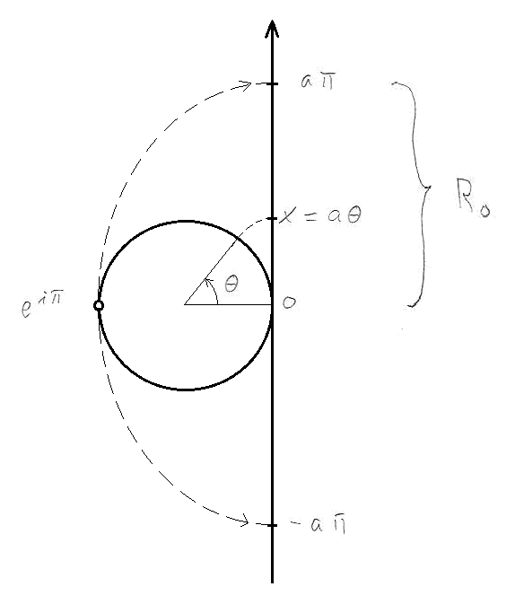
Figure 1: Projection from configuration space to laboratory space.

Now a shortest geodesic (Milnor, ) to track along the full extension of the u(3) maximal torus runs from the origin at $u=I$ where all eigenvalues are $1=e^{i0}$ to $u=-I$ where all eigenvalues are $-1=e^{i\pi}$, see also fig. 1. When for instance the neutron decays to the proton - and the electron is created as a ”peel off” - the topological change in the interior baryon state maps by projection to laboratory space. It is not a new idea to suggest the classical electron radius as a fundamental length in elementary particle physics (HeisenbergMehra, ; Heisenberg, ). Here we specify the introduction of the scale (3) via the projection (5). Conjugate to the space (angle) parameters in (5) are canonical momentum (action) operators

$$p_{j}=-i\hbar\frac{1}{a}\frac{\partial}{\partial\theta_{j}}=\frac{\hbar}{a}T_{j}.$$ (6)

The toroidal generators $T_{j}$ induce coordinate fields $\partial_{j}$ according to the above mentioned eigenangle parametrization of the u(3) torus. In general the nine generators $T_{k}$ of u(3) namely induce coordinate fields as follows

$$\partial_{k}=\frac{\partial}{\partial\theta}ue^{i\theta T_{k}}|_{\theta=0}=uiT_{k}.$$ (7)

The remaining six off-toroidal generators are important in the baryon spectroscopy phenomenology resulting from (2) since they take care of spin and flavour degrees of freedom. With these parametrizations the Laplacian ($\hbar=1$) in a polar decomposition reads (Wadia, ; TrinhammerOlafsson, )

$$\Delta=\sum^{3}_{j=1}\frac{1}{J^{2}}\frac{\partial}{\partial\theta_{j}}J^{2}\frac{\partial}{\partial\theta_{j}}-\!\!\!\sum^{3}_{\begin{subarray}{c}i<j\\ k\neq i,j\end{subarray}}\frac{K^{2}_{k}+M^{2}_{k}}{8\sin^{2}\frac{1}{2}(\theta_{i}-\theta_{j})}$$ (8)

Here the Van de Monde determinant, the ”Jacobian” of the parametrization is Weyl

$$J=\prod^{3}_{i<j}2\sin\left(\frac{1}{2}(\theta_{i}-\theta_{j})\right).$$ (9)

The operators $K_{k}$ commute as body fixed angular momentum operators and $M_{k}$ ”connect” the algebra by commuting into the subspace of $K_{k}$

$$[M_{k},M_{l}]=[K_{k},K_{l}]=-iK_{m},$$ (10)

cyclic in $k,l,m$. The presence of the components of ${\bf{K}}=(K_{1},K_{2},K_{3})$ and ${\bf{M}}=(M_{1},M_{2},M_{3})$ in the Laplacian opens for the inclusion of spin and flavour. Interpreting $\bf{K}$ as the interior spin operator is encouraged by the body fixed signature of the commutation relations. The relation between laboratory space and interior space is like the relation in nuclear physics between fixed coordinate systems and intrinsic body fixed coordinate systems for the description of rotational degrees of freedom. To derive the spectrum for $M^{2}$ we use a coordinate representation (Schiff, )

$$K_{1} =a\theta_{2}p_{3}-a\theta_{3}p_{2}=\hbar\lambda_{7}$$

$$K_{2} =a\theta_{1}p_{3}-a\theta_{3}p_{1}=\hbar\lambda_{5}$$

$$K_{3} =a\theta_{1}p_{2}-a\theta_{2}p_{1}=\hbar\lambda_{2}.$$ (11)

and

$$M_{3}/\hbar =\theta_{1}\theta_{2}+\frac{a^{2}}{{\hbar}^{2}}p_{1}p_{2}=\lambda_{1}$$

$$M_{2}/\hbar =\theta_{3}\theta_{1}+\frac{a^{2}}{{\hbar}^{2}}p_{3}p_{1}=\lambda_{4}$$

$$M_{1}/\hbar =\theta_{2}\theta_{3}+\frac{a^{2}}{{\hbar}^{2}}p_{2}p_{3}=\lambda_{6}.$$ (12)

The lambdas are corresponding Gell-Mann generators (SchiffOpCit, ). From these and

$$Y/\hbar=\frac{1}{6}(\theta^{2}_{1}+\theta^{2}_{2}-2\theta^{2}_{3})+\frac{1}{6}\frac{a^{2}}{{\hbar}^{2}}(p^{2}_{1}+p^{2}_{2}-2p^{2}_{3})=\lambda_{8}/\sqrt{3},$$

$$2I_{3}/\hbar=\frac{1}{2}(\theta_{1}^{2}-\theta^{2}_{2})+\frac{1}{2}\frac{a^{2}}{{\hbar}^{2}}(p_{1}^{2}-p^{2}_{2})=\lambda_{3}$$ (13)

we find by straightforward but tideous commutations the spectrum

$$M^{2}=\frac{4}{3}(n+\frac{3}{2})^{2}-K(K+1)-3-\frac{1}{3}y^{2}-4i^{2}_{3},$$

$$n=0,1,2,3,\dots$$ (14)

where $y$ and $i_{3}$ are hypercharge and isospin three-component quantum numbers. The minimum value for the positive definite $M^{2}$ is 13/4 in the case of spin 1/2, hypercharge 1 and isospin 1/2 as for the nucleon. To solve for the eigenvalues we factorize the wavefunction

$$\Psi(u)=\tau(\theta_{1},\theta_{2},\theta_{3})\Upsilon(\alpha_{4},\alpha_{5},\alpha_{6},\alpha_{7},\alpha_{8},\alpha_{9}),$$ (15)

insert it in (2) and then integrate over the off-toroidal degrees of freedom $(\alpha_{4},\alpha_{5},\alpha_{6},\alpha_{7},\alpha_{8},\alpha_{9})$ to get for the measure scaled wavefunction $R=J\tau(\theta_{1},\theta_{2},\theta_{3}),$ for toroidal degrees of freedom

$$\left[-\sum^{3}_{j=1}\frac{\partial^{2}}{\partial\theta_{j}^{2}}+V\right]R=2{\rm{E}}R.$$ (16)

Here

$$V=-2+\frac{1}{3}(K(K+1)+M^{2})\sum^{3}_{i<j}\frac{1}{8\sin^{2}\frac{1}{2}(\theta_{i}-\theta_{j})}$$

$$\hskip 28.45274pt+2(v(\theta_{1})+v(\theta_{2})+v(\theta_{3})).\hskip 71.13188pt$$ (17)

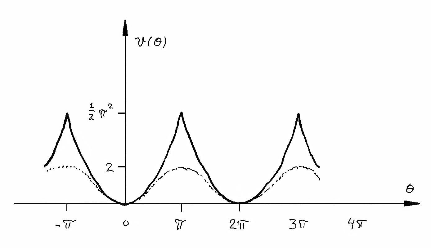
Figure 2: Periodic parametric potential (1 The mass ratio and the model) originating from the potential in (2). The dashed curve corresponds to the Wilson analogue (Wilson, ) of the Manton action and is not considered in the present work.

where (see fig. 2)

$$v(\theta)=\frac{1}{2}(\theta-n\cdot 2\pi)^{2},\quad\theta\in[(2n-1)\pi,(2n+1)\pi],$$

$${\rm{for}}\quad n\in Z.\hskip 113.81102pt$$ (18)

By expansion on Slater determinants Wadia

$$b_{pqr}=\epsilon_{ijk}\cos(p\theta_{i})\sin(q\theta_{j})\cos(r\theta_{k})$$ (19)

with integer $p,q,r$, we can solve (16) by a Rayleigh Ritz method BruunNielsen to yield the ground state eigenvalue ${\rm{E_{0}}}=4.38$ which corresponds to $m_{e}/m_{0}=1/1885$. This is less than three percent off the value $m_{e}/m_{n}=1/1838.6...$ based on experimental data for the electron and neutron Beringer . Note that $b_{pqr}$ is antisymmetric in the colour degrees of freedom $\theta_{j}$.

2 Parton distribution functions

We can generate parton distribution functions by projections via the momentum form, i.e. the exterior derivative on the u(3) manifold. For this we expand the exterior derivative $dR$ of the measure scaled toroidal wavefunction $R$ on the torus forms $d\theta_{j}$,

$$dR=\psi_{j}d\theta_{j}.$$ (20)

The action of the torus forms on the toroidal coordinate fields expresses the generalization to the interior configuration space manifold of the quantization inherent in the conjugate variables in (5) and (6), thus

$$d\theta_{i}(\partial_{j})=\delta_{ij}\Leftrightarrow[\partial_{j},\theta_{i}]=\delta_{ij}$$ (21)

Inspired by Bettini’s elegant treatment of parton scattering Bettini we generate distribution functions via our exterior derivative. The derivation runs like this (with $\hbar=c=1$): Imagine a proton at rest with four-momentum $P=({\text{\bf{0}}},E_{0})$. We boost it virtually to energy $E$ by impacting upon it a massless four-momentum $q=({\text{\bf{q}}},E-E_{0})$ which we assume to hit a parton $xP$. After impact the parton represents a virtual mass $xE$. Thus

$$(xP_{\mu}+q_{\mu})\cdot(xP^{\mu}+q^{\mu})=x^{2}E^{2},$$ (22)

from which we get the parton momentum fraction

$$x=\frac{2E_{0}}{E+E_{0}},$$ (23)

or the boost parameter

$$\xi\equiv\frac{E-E_{0}}{E}=\frac{2-2x}{2-x}.$$ (24)

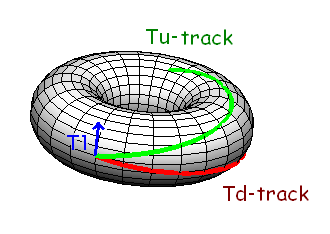
Figure 3: The generators $T_{u}$ and $T_{d}$ given in (28) generate traces along the u(3) torus as shown here in the first and third toroidal degrees of freedom with $T_{3}$ pointing to the left.

We can use the boost parameter for an angular track $\theta=\pi\xi$ on the manifold in the direction laid out by a specific toroidal generator

$$T=a_{1}T_{1}+a_{2}T_{2}+a_{3}T_{3}.$$ (25)

With the toroidal generator $T$ as introtangling momentum operator we namely have the qualitative correspondence $q_{\mu}\sim E-E_{0}\sim(1-x)E\sim(1-x)T$. That is, we will project along $\xi T\sim(1-x)T$ in order to probe on $xP_{\mu}$. With a probability amplitude interpretation of $R$ we project on a fixed colour base $iT_{j}$ and sum over the colour components for a specific generator $T$ to get the corresponding distribution function $f_{T}(x)$ determined by

$$f_{T}(x)dx=(\sum^{3}_{j=1}dR_{u=exp(\theta iT)}(iT_{j}))^{2}d\theta$$ (26)

By a pull-back operation GuilleminPollack to parameter space we get

$$\sum^{3}_{j=1}dR_{u=\exp(\theta iT)}(iT_{j})=dR_{u=\exp(\theta iT)}(i(T_{1}+T_{2}+T_{3}))$$

$$=\frac{d}{dt}R(ue^{ti(T_{1}+T_{2}+T_{3})}){\text{\Large{$\mid$}}}_{t=0}$$

$$=\frac{d}{dt}R(a_{1}\theta+t,a_{2}\theta+t,a_{3}\theta+t){\text{\Large{$\mid$}}}_{t=0}$$

$$=\sum^{3}_{j=1}\frac{\partial R}{\partial\theta_{j}}{\text{\Large{$\mid$}}}_{(\theta_{1},\theta_{2},\theta_{3})=(\theta\cdot a_{1},\theta\cdot a_{2},\theta\cdot a_{3})}\cdot\frac{\partial(a_{j}\theta+t)}{\partial t}{\text{\Large{$\mid$}}}_{t=0}$$

$$=\left(\frac{\partial R}{\partial\theta_{1}}+\frac{\partial R}{\partial\theta_{2}}+\frac{\partial R}{\partial\theta_{3}}\right){\text{\Large{$\mid$}}}_{(\theta_{1},\theta_{2},\theta_{3})=(\theta\cdot a_{1},\theta\cdot a_{2},\theta\cdot a_{3})}$$

$$\equiv D(\theta\cdot a_{1},\theta\cdot a_{2},\theta\cdot a_{3}).$$ (27)

Along the tracks shown in fig. 3, we generate distributions by

$$T_{u}=\begin{Bmatrix}2/3&0&0\\ 0&0&0\\ 0&0&-1\end{Bmatrix}\hskip 5.69054pt\text{and}\hskip 5.69054ptT_{d}=\begin{Bmatrix}-1/3&0&0\\ 0&0&0\\ 0&0&-1\end{Bmatrix}\!.$$ (28)

as shown in fig. 4 for a first order approximation

$$b_{0,\frac{1}{2},1}(\theta_{1},\theta_{2},\theta_{3})=\frac{1}{N}\begin{vmatrix}1&1&1\\ \sin\frac{1}{2}\theta_{1}&\sin\frac{1}{2}\theta_{2}&\sin\frac{1}{2}\theta_{3}\\ \cos\theta_{1}&\cos\theta_{2}&\cos\theta_{3}\end{vmatrix}\!,$$ (29)

to an expansion for a protonic state with normalization constant $N$. For instance

$$xf_{Tu}(x)=x\left[D\left(\pi\frac{2-2x}{2-x}\cdot\frac{2}{3},\pi\frac{2-2x}{2-x}\cdot 0,\pi\frac{2-2x}{2-x}\cdot(-1)\right)\right]^{2}\cdot\frac{\pi\cdot 2}{(2-x)^{2}}.$$ (30)

where in its full glory

$$ND(\theta_{1},\theta_{2},\theta_{3})=\hskip 170.71652pt$$

$$-\frac{1}{2}\cos\frac{\theta_{1}}{2}\cdot(\cos\theta_{3}-\cos\theta_{2})-\sin\theta_{1}\cdot(\sin\frac{\theta_{3}}{2}-\sin\frac{\theta_{2}}{2})$$

$$+\frac{1}{2}\cos\frac{\theta_{2}}{2}\cdot(\cos\theta_{3}-\cos\theta_{1})+\sin\theta_{2}\cdot(\sin\frac{\theta_{3}}{2}-\sin\frac{\theta_{1}}{2})$$

$$-\frac{1}{2}\cos\frac{\theta_{3}}{2}\cdot(\cos\theta_{2}-\cos\theta_{1})-\sin\theta_{3}\cdot(\sin\frac{\theta_{2}}{2}-\sin\frac{\theta_{1}}{2}).$$ (31)

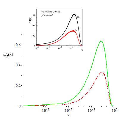
Figure 4: Parton distribution functions from a first order approximation to the ground state of (2) as a function of the parton fraction $x$. The distributions are generated by impact along $T_{u}=(2/3,0,-1)$ (solid, green line) and $T_{d}=(-1/3,0,-1)$ (dashed, red line) with no fitting parameters. For comparison we show $u$ and $d$ valence quarks of the proton at 10 GeV² in the insert adapted from the particle data group with other parton distributions erased Beringer .

The distribution functions shown in fig.4 contain no fitting parameters at all. Note that the $T_{u}$-parton momentum content of the approximate state (29) is close to the double of the $T_{d}$-content

$$\int^{1}_{0}xf_{Tu}(x)dx\,{\text{\Large{/}}}\int^{1}_{0}xf_{Td}(x)dx$$

$$=0.2722{\text{\Large{/}}}0.1437=1.89\approx 2,$$ (32)

Work is in progress to solve (2) for the charged proton by antisymmetrized parity definite expansions on Bloch states Jacobsen

$$g_{pqr}=e^{i\mbox{\boldmath{$\kappa$}}\cdot\mbox{\boldmath{$\theta$}}}e^{ip\theta_{1}}e^{iq\theta_{2}}e^{ir\theta_{3}},$$ (33)

where $\kappa$ $=(\kappa_{1},\kappa_{2},\kappa_{3})$ are appropriately chosen Bloch vectors and $\theta$ $=(\theta_{1},\theta_{2},\theta_{3})$ .

3 Comments

It is not clear whether the minor but still significant discrepancy in our value for $m_{e}/m_{n}$ is due to disparate partial wave projections of the base set (19) or due to corrections needed in (3). It is somewhat surprising that when applied to a neutral state expression (1) gives a result just three percent off the experimental value for the electron to neutron value. This is surprising since the classical electron radius on which we base our prediction is normally presented to be just an order of magnitude scale for strong interaction phenomena HeisenbergOpCit . It should be noted though that in (5) we have introduced a well defined projection to space parameters. However, at the present level of understanding it seems wise to quote L. D. Landau and E. M. Lifshitz: ”…it is impossible within the framework of classical electrodynamics to pose the question whether the total mass of the electron is electrodynamic.” LandauLifshitz

Conclusion

We have derived an expression for the electron to nucleon mass ratio from a reinterpreted lattice gauge theory Hamiltonian. A specific calculation for the neutron from expansions on Slater determinants of indefinite parity gives a result less than three percent off the experimental value. The proximity of prediction to observation should encourage further study within the framework of the Hamiltonian model presented. From the same model we have derived approximate parameter free parton distribution functions that compare rather well with those for the $u$ and $d$ valence quarks of the proton. Work is in progress to establish a complete Bloch wave base for expansions with suitable symmetry requirements implied by the potential and the antisymmetry under interchange of colour degrees of freedom.

References

References

- [1] J. J. Sakurai, Advanced Quantum Mechanics, 10th printing, (Addison-Wesley, United Kingdom 1967/1984), p. 12.
- [2] J. B. Kogut and L. Susskind, Hamiltonian formulation of Wilson’s lattice gauge theories, Phys. Rev. D11 (2), 395, (1975).
- [3] N. S. Manton, An Alternative Action for Lattice Gauge Theories, Phys. Lett. B96, 328-330 (1980).
- [4] O. Trinhammer, Infinite N phase transitions in one-plaquette (2+1)-dimensional models of lattice gauge theory with Manton’s action, Phys. Lett. B129 (3, 4), 234-238 (1983).
- [5] L. D. Landau and E. M. Lifshitz, The Classical Theory of Fields, Course of Theoretical Physics Vol. 2, 4th ed., (Elsevier Butterworth-Heinemann, Oxford 2005), p.97.
- [6] J. Milnor, Morse Theory, Ann. of Math. Stud. 51, 1 (1963).
- [7] W. Heisenberg, Über die in der Theorie der Elementarteilchen auftretende universelle Länge, Ann. d. Phys. (5) 32, 20-33. (1938).
- [8] J. Mehra and H. Rechenberg, The Historical Development of Quantum Theory - The Conceptual Completion and the Extensions of Quantum Mechanics 1932-1941, Vol. 6, Part 2, (Springer, New York 2001). p.956.
- [9] O. L. Trinhammer and G. Olafsson, The Full Laplace-Beltrami operator on U(N) and SU(N), arXiv:math-ph/9901002v2 (1999/2012).
- [10] S.R. Wadia, N = Phase Transition in a Class of Exactly Solvable Model Lattice Gauge Theories, Phys. Lett. B93, 403-410 (1980).
- [11] H. Weyl, The Classical Groups - Their Invariants and Representations, (Princeton University Press, 1939, 2nd ed. 15th printing 1997), p.197.
- [12] L. I. Schiff, Quantum Mechanics, 3rd ed. (McGraw-Hill 1968), p. 211.
- [13] See ref. [[12]], p. 209.
- [14] K. G. Wilson, Confinement of quarks, Phys. Rev. D10, 2445-2449 (1974).
- [15] H. Bruun Nielsen, Technical University of Denmark, (private communication, 1997).
- [16] J. Beringer et al. (Particle Data Group), Review of Particle Physics, Phys. Rev. D86, 010001 (2012), p.30, p.79.
- [17] A. Bettini, Introduction to Elementary Particle Physics, (Cambridge University Press, UK 2008), p.204.
- [18] W. Guillemin and A. Pollack, Differential Topology, (Prentice-Hall, New Jersey, USA 1974), p.163.
- [19] Karsten W. Jacobsen, Technical University of Denmark, (private communication, June 2012).
- [20] See ref. [[7]], p. 20.