Relaxation of flying spin qubits in quantum wires by hyperfine interaction

Abstract

We consider the relaxation of a spin qubit in a quantum dot propagating as a whole in a one-dimensional semiconductor with hyperfine coupling. We show that this motion leads to qualitatively new features in this process compared to static quantum dots. For a fast straightforward motion, the initial spin density decreases to zero with the relaxation rate independent of the spatial spread of the electron wave function and inversely proportional to the electron speed. However, for the oscillatory motion, the qubit acquires memory, and the dephasing becomes Gaussian rather than exponential. After some time, one third of the initial spin polarization is restored, as it happens for static qubits. This revival can occur either through periodic peaks or through a monotonous increase in the polarization, after a minimum, until a plateau has been reached. Our results can be useful for the understanding of the spin dynamics and decoherence in quantum wires.

Semiconductor quantum wires play an important role in fundamental and applied spintronics. They allow one to study a variety of interesting phenomena related to spin transport Pramanik ; Kiselev ; Quay ; Bringer ; Governale ; Pershin ; Holleitner ; Sanchez ; Lu ; Romano ; Japaridze and open the way to realizations of exotic states such as Majorana fermions Mourik12 ; Gangadharaiah .

One of the most interesting aspects of spintronics is the hyperfine coupling of spins of carriers to the nuclear magnetic moments of the host lattice Glazov12 ; Greilich ; Coish ; LianAo ; Marcus1 ; Dahbashi , strongly dependent on the spatial extension of the carriers wave functions. In semiconductor nanostructures, it is enhanced compared to the bulk due to confined wave functions in quantum dots Merkulov ; Braun ; Raith and due to localization by disorder in quantum wires.Echeverria2 The spin dephasing times observed in quantum dots Braun agree very well with what can be expected from the theory.Merkulov

The observed relaxation times suggest that a single electron spin could become the physical realization of a quantum bit (qubit), crucial for quantum information applications. Unlike the dots, where electrons are well localized, extended nanowires are natural channels for traveling qubits, hereafter referred to as ”flying” qubits Yamamoto ; Nadj . Spin decoherence is the major concern for using qubits in information processing. At low temperatures, it is mainly caused by spin-orbit and hyperfine interactions. In undoped wires, the mechanisms for spin-orbit relaxation can be canceled out by tuning their cross section geometries for the wires extended along the [001] direction (Dresselhaus term) and also by keeping their environments symmetric (Rashba term). Hyperfine couplings hence can become the only source of spin depolarization. Their influence on the spin dynamics of qubits propagating through nanowires should be deeply understood for spin transport devices. Recently, Huang and Hu Hu have proposed a formulation of the spin-relaxation problem well suited for quantum information purposes. This formulation comes from studying the decoherence of an electron spin that is being transported in a random electric potential, as enclosed in a quantum dot with the time-independent shape of the wave function. The ability of high-fidelity electron transfer between quantum dots by surface acoustic waves was demonstrated recently.Stotz ; Hermelin ; McNeil ; Sanada Here we apply a similar approach to study the effects of hyperfine interaction on spins in moving quantum dots, and show that the dynamics brings about new time scales and qualitative features compared to the static dots.

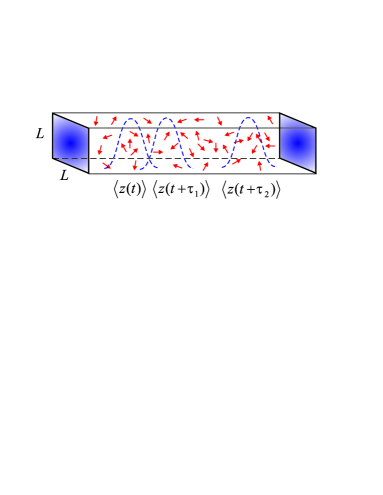
Figure 1: (Color online) Schematic plot of a semiconductor quantum wire. Random arrows show the magnetic moments of nuclei. Dashed lines correspond to density distributions with given expectation values of the $z$ coordinate at different times: For $\tau_{1}$, of the order of $\tau_{\xi}$, the matching of tails yields some correlation; for $\tau_{2}$, considerably larger than $\tau_{\xi}$, correlation is negligible.

We consider nanowires with $L\times L$ cross section, see Fig. 1, and we take GaAs as a representative spintronics material. Nuclear magnetic moments are considered frozen on the time scale of the electron precession Merkulov , and are represented as random $I=3/2$ spins with the expectation values of components $I_{i}$, where $i=x,y,z$. Under the assumption of decoupled spin and orbital motion, valid in the absence of spin-orbit coupling and for weak hyperfine interaction, we can factorize the total wave function as $\psi(\mathbf{r},t)\left|\phi\rangle\right.$. Here the orbital state is $\psi(\mathbf{r},t)$ and the spinor state is $\left|\phi\rangle\right.$. The resulting Hamiltonian for the spin degree of freedom depends on the orbital wave function as follows:

$$\hat{H}_{\text{hf}}=\frac{A\nu}{2}\sum_{n}|\psi(\mathbf{r}_{n},t)|^{2}(I_{x}^{[n]}\sigma_{x}+I_{y}^{[n]}\sigma_{y}+I_{z}^{[n]}\sigma_{z}),$$ (1)

where the summation goes over all nuclei with spin components $I_{i}^{[n]}$ at sites $\mathbf{r}_{n}$, $A$= 45 $\mu$eV is the typical hyperfine coupling constant for GaAs Merkulov , $\nu$ is the volume per single nucleus (one eighth of the unit cell), and $\sigma_{i}$ are the Pauli matrices.

Hamiltonian (1) can be rewritten in the form

$$\hat{H}_{\text{hf}}=\frac{\hbar}{2}\left({\bm{\Omega}}\cdot{\bm{\sigma}}\right),$$ (2)

where the precession due to hyperfine interaction $\mathbf{\Omega}$ is an integral that depends on the electron position and can be expressed as

$$\Omega_{i}=\frac{A\nu}{\hbar}\int_{V}|\psi(\mathbf{r},t)|^{2}\rho_{i}(\mathbf{r})dV.$$ (3)

Here the density of the $i$-th component of the nuclear magnetic moment $\rho_{i}(\mathbf{r},t)$ satisfies the white-noise distribution $\left\langle\langle\rho_{i}(\mathbf{r})\rho_{i}(\mathbf{r}^{\prime})\right\rangle\rangle=\rho_{0}\delta\left(\mathbf{r-r}^{\prime}\right),$ where $\langle\langle\ldots\rangle\rangle$ stands for the ensemble average and $\rho_{0}=\langle\hat{I}_{i}^{2}\rangle/\nu$; here $\nu^{-1}$ is the concentration of nuclei. To describe a moving electron, we need the characteristic time-dependent correlator which can be obtained, assuming Gaussian random fluctuations Shklovskii ; Glazov05 , as:

$$\frac{\hbar^{2}}{\left(A\nu\right)^{2}}\left\langle\langle\Omega_{i}(t)\Omega_{i}(t+\tau)\right\rangle\rangle=$$ (4)

$$\int\int|\psi(\mathbf{r}_{1},t)|^{2}|\psi(\mathbf{r}_{2},t+\tau)|^{2}\left\langle\langle\rho_{i}(\mathbf{r}_{1})\rho_{i}(\mathbf{r}_{2})\right\rangle\rangle dV_{1}dV_{2}$$

$$=\rho_{0}\int\int|\psi(\mathbf{r},t)|^{2}|\psi(\mathbf{r},t+\tau)|^{2}dV.$$

Although, due to the isotropy of the random distribution of nuclear spins, these correlators are $i-$independent, for definiteness we consider the $z-$ component of the spin below. With the course of time, the overlap of the electron wave function with itself decreases and the correlation gradually vanishes, as can be realized from Fig.1. The $\psi(\mathbf{r}_{n},t)$ states characterizing the propagating qubits are defined as $\psi(\mathbf{r}_{n},t)=\eta(z_{n},t)\varphi(x_{n},y_{n})$, where $\varphi(x_{n},y_{n})=(2/L)\sin(\pi x_{n}/L)\sin(\pi y_{n}/L)$ describes an electron in a single-mode box, and $\eta(z_{n},t)$ is assumed to be a Gaussian centered at the time-dependent position $\langle z(t)\rangle$, corresponding to the ground state of the moving parabolic potential:

$$\eta(z_{n})=\left(\frac{1}{2\pi\xi^{2}}\right)^{1/4}\exp\left[{-(z_{n}-\langle z(t)\rangle)^{2}/4\xi^{2}}\right].$$ (5)

For this choice of the wave function, the correlator in Eq.(4) is expressed as

$$\left\langle\langle\Omega_{i}(t)\Omega_{i}(t+\tau)\right\rangle\rangle=\left\langle\langle\Omega_{i}^{2}\right\rangle\rangle\exp\left[-\left(\Delta z(\tau)\right)^{2}/4\xi^{2}\right],$$ (6)

where $\langle\langle\Omega_{i}^{2}\rangle\rangle=3\left(A/\hbar\right)^{2}I(I+1)\nu/8\sqrt{\pi}L^{2}\xi$ and $\Delta z(\tau)\equiv\langle z(t+\tau)\rangle-\langle z(t)\rangle$. This correlator reaches the maximum when the electron is back to the position occupied at time $t$. For motion with constant speed, $\Delta z(\tau)=v\tau$ and the corresponding effective correlation time can be defined as $\tau_{\xi}\equiv\xi/v$.

Now we analyze the evolution of polarization of static and propagating wave packets. The spin dynamics is calculated for ensembles of random wires and averaged afterwards. At the initial time, qubits are fully polarized in the nonequilibrium spin state $|\phi(0)\rangle=|1\rangle$. Later on, for $t>0$, $|\phi(t)\rangle$ evolves following the time dependent Schrödinger equation,

$$i\hbar\frac{\partial\left|\phi\right>}{\partial t}=\hat{H}_{\text{hf}}(t)\left|\phi\right>,$$ (7)

where the time dependence of $\hat{H}_{\text{hf}}(t)$ is due to the displacement of the qubit. The resulting spinor $|\phi(t)\rangle$ is related to the initial spin state as

$$|\phi(t)\rangle=\mathcal{T}\exp\left[-\frac{i}{\hbar}\int_{0}^{t}\hat{H}_{\text{hf}}(t)dt\right]|\phi(0)\rangle,$$ (8)

where $\mathcal{T}$ stands for the time ordering.

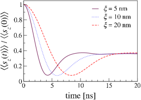
Figure 2: (Color online) Spin dynamics of static qubits for different width $\xi$ as solved by $4^{\mathrm{th}}-$order Runge-Kutta method and averaged over 4096 realizations of disorder in the nuclear magnetic moments with the statistical errors of the order of $1/\sqrt{4096}=1.6\%$. Here and below we assume the wire width $L=8$ unit cells. For this wire width and $\xi=10$ nm, we obtain $1/\sqrt{\langle\langle\Omega_{i}^{2}\rangle\rangle}\approx 1.5$ ns, corresponding well to the relaxation time in the Figure. Since the GaAs lattice constant is $0.565$ nm, the nanowire cross-section is $4.5\times 4.5\simeq 20$ nm².

We consider three different realizations of spin dephasing: for static qubits (to have the known system to compare with), and for straightforward and oscillatory motion. When packets are fixed to initial positions, the calculated average polarization decays to a minimum of about 0.1 of the initial value and monotonically increases up to a constant plateau where $\langle\langle s_{z}(t)\rangle\rangle=\langle\langle s_{z}(0)\rangle\rangle/3$. We consider packets with widths of $\xi=5$, 10, and 20 nm; their spin evolutions, plotted in Fig. 2, look exactly as expected from the dynamics induced by hyperfine coupling in quantum dots Merkulov ; Echeverria2 . This steady polarization arises due to the precessional motion of the qubit spin around the time-independent effective field of the nuclear magnetic moments Merkulov . The spin evolution presented in this Figure is universal in the sense that it can be fully described by two timescales originated from the same random position-dependent spin precession: that for the initial polarization to decay down to $1/e$, and that for reaching the 1/3 plateau. The scale for the initial decay rate of static electrons is then $\Gamma_{\rm st}=\sqrt{\langle\langle\Omega_{i}^{2}\rangle\rangle}$, and the entire time dependence in Fig. 2 can be described by using this single parameter Merkulov . The dependence of the spin dynamics on the qubit spatial width is related to the number of interacting nuclei inside the electron cloud: A smaller amount of nuclei yields stronger fluctuations in the field resulting in a faster decay.

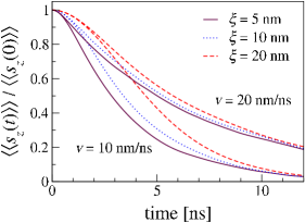
Figure 3: (Color online) Average polarization for qubits in straightforward motion for different speeds $v$ and widths $\xi$.

In the next, straightforward motion regime, packets propagate along the wire with constant velocities $v=10$ and $20$ nm/ns, taken here as examples. A behavior considerably different from the static one emerges when $\tau_{\xi}\Gamma_{\rm st}$ is much less than 1, that is, when the electron moves to a strongly different realization of the hyperfine field before sufficiently changing its spin; this behavior is shown in Fig. 3. To gain insight into the influence of width and speed, we have taken into account, again, three distinct packet sizes, $\xi=5$, 10, and 20 nm. When $v=10$ nm/ns all polarizations decrease below 0.1 after 10 ns and monotonically tend to zero afterwards. In addition, the smaller the qubit width, the faster the dephasing. Similar calculations for $v=20$ nm/ns show a considerably less efficient decoherence. This behavior can be detailed as follows. The average spin evolution can be described with Glazov05

$$\frac{\left\langle\langle s_{z}(t)\right\rangle\rangle}{\left\langle\langle s_{z}(0)\right\rangle\rangle}=\exp\left[-\int_{0}^{t}dt^{\prime}\int_{0}^{t^{\prime}}\langle\langle\Omega_{z}(t^{\prime})\Omega_{z}(t^{\prime}-t^{\prime\prime})\rangle\rangle dt^{\prime\prime}\right].$$ (9)

For the exponentially decaying part of the dynamics, this expression has the form

$$\frac{\left\langle\langle s_{z}(t)\right\rangle\rangle}{\left\langle\langle s_{z}(0)\right\rangle\rangle}=\exp(-\sqrt{\pi}\Gamma_{v}t),$$ (10)

where the spin relaxation rate is determined by

$$\Gamma_{v}=\langle\langle{\Omega}_{i}^{2}\rangle\rangle\tau_{\xi}.$$ (11)

Therefore, the fast motion establishes a new and smaller relaxation rate, $\Gamma_{v}=\Gamma_{\rm st}\cdot\left(\Gamma_{\rm st}\tau_{\xi}\right)$, such as $\Gamma_{v}\ll\Gamma_{\rm st}$. Here $\Gamma_{v}$ does not depend on the width of the electron wave packet but only on its speed, as we explain below using a scaling argument. The electron spin precession rate, due to the frozen nuclear spins, is of the order of $\Omega\sim\left(A/\hbar\right)/\sqrt{N},$ where the number of nuclear magnetic moments per single electron is $N\sim L^{2}\xi/\nu$. From Eq.(11), the resulting $\Gamma_{v}$ is proportional to $\left(A/\hbar\right)^{2}\nu/L^{2}v$ and, henceforth, also $\xi-$independent. This argument can easily be applied to other spatial dimensions $D$ in the following way. The square of the spin precession rate being of the order of $\langle\langle\Omega_{i}^{2}\rangle\rangle\sim N^{-1}\sim\xi^{-D},$ while $\tau\sim\xi/v$, is $D-$independent. As a consequence, $\Gamma_{v}\sim\xi^{1-D}/v$, which tends to zero for bulk crystals ($D=3$) and two-dimensional structures ($D=2$) when the size of the wave packet is increased. However, it remains constant in the wires ($D=1$), making the results only weakly dependent on the details of the electron wave function, provided that it broadens relatively slow, on the timescale of spin precession in the hyperfine field, such that the fast motion condition $\tau_{\xi}\Gamma_{\rm st}\ll 1$ holds. We notice that, for the electrons transferred by the surface acoustic waves Stotz ; Hermelin ; McNeil ; Sanada with the speed close to $3\times 10^{3}$ nm/ns, the condition of fast motion is well satisfied for $\xi$ up to 500 nm. As a result, the spin states are well protected against relaxation.

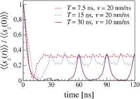
Figure 4: (Color online) Average polarization for qubits flying back and forth along the wires for various speeds and periods, $\xi=10$ nm. Note the sharp revivals in the regime when $T=30$ ns and $v=10$ nm/ns.

A significantly different behavior is obtained when the packet moves back and forth, in a regime which can be experimentally achieved by the surface acoustic wave technique.McNeil We analyze oscillations with different velocities and frequencies, which make amplitudes in the range of several tens of nanometers. We assume that the expectation value of the qubit $z-$coordinate follows a saw-like function,

$$\left\langle z(t)\right\rangle=2\ell\left|\frac{t}{T}-\left\lfloor\frac{t}{T}+\frac{1}{2}\right\rfloor\right|,$$ (12)

where $\lfloor\ldots\rfloor$ stands for the floor function, $T$ is the period, and $\ell=vT/2$ is the maximum displacement from the initial position. Every time the electron returns to the initial position, once per period, it scans exactly the same effective field. As a consequence, the spin dynamics experiences strong correlations which yield the memory effects. In the oscillatory regime, the correlator for the precession rate satisfies the conditions $\left\langle\langle\Omega_{i}(t)\Omega_{i}(T(\left\lfloor 2t/T\right\rfloor+1)-t)\right\rangle\rangle=\left\langle\langle\Omega_{i}^{2}\right\rangle\rangle$ and $\left\langle\langle\Omega_{i}(t)\Omega_{i}(t+nT)\right\rangle\rangle=\left\langle\langle\Omega_{i}^{2}\right\rangle\rangle$, where $n\geq 0$ is an integer.

We begin with the regime where $T\Gamma_{v}$ is of the order of 1 and the typical electron spin strongly changes in a single oscillation. The spin polarization behavior is shown in Fig. 4. We begin with the period $T=7.5$ ns and velocity $v=20$ nm/ns, where spin relaxation during half a period is not very strong yet. As a result, the polarization first decays and then increases to a stable value with tiny saw-like peaks on the top. For a twice larger period, $T=15$ ns and $v=20$ nm/ns, the product $T\Gamma_{v}$ is larger by a factor of 2, spin relaxation per period is considerably more efficient, and the calculated dynamics already presents clear periodic peaks above the reached plateau. For a yet smaller frequency and speed, $T=30$ ns and $v=10$ nm/ns, one observes an almost flat stage followed by a series of sharp revivals periodically repeated in time, see Fig. 4. Here, in the first period, the polarization relaxes down to zero. Throughout the second period, the qubits show a revival to 1/3 of the initial spin. Beyond two periods, relaxation and memory effects both contribute to yield a periodic picture of revivals up to one third and decays down to zero.

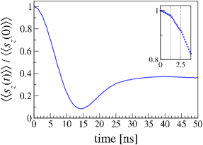
Figure 5: (Color online) Average polarization of an oscillating qubit when $T=2.5$ ns, $v=160$ nm/ns, and $\xi=10$ nm. The inset shows details of the short-term behavior changing slope every half a period shown by vertical dotted lines.

In the next case, we consider very high velocity and frequency, $T\Gamma_{v}\ll 1$, resulting in a small spin precession angle in one period. When $v=160$ nm/ns and $T=2.5$ ns, the average spin polarization decays to a minimum of about 10% of the initial value and monotonically increases up to a constant plateau of 1/3; the ensemble dephasing time is roughly 14 ns, as can be seen in Fig. 5. Due to the extremely high speed, the qubit spin cannot follow, by precessional motion, the fast changes in the effective nuclear magnetic field. The characteristic behavior is given in Fig. 5, similar to that depicted in Fig. 2 for static qubits. Here, the behavior of polarization in time cannot be modified by tuning the qubit width.

In the oscillatory regime, the relaxation part of the time-dependence is Gaussian rather than exponential Glazov05 ; Reuther , as we explain below. At any $t$, ensemble mean value of spin $z-$ component is $\left\langle\langle\cos\theta_{z}\right\rangle\rangle/2$, where $\theta_{z}$ is the corresponding precession angle; this mean value is $\left\langle\langle\cos\theta_{z}\right\rangle\rangle=\exp(-\sqrt{\pi}\Gamma_{v}t)$ for $0<t<T/2$, and is multiplied by factor $n$, $\left\langle\langle\cos\theta_{z}\right\rangle\rangle=\exp(-\sqrt{\pi}n^{2}\Gamma_{v}t)$, at $t=nT/2$. Thus, in this regime, a new spin relaxation rate is established, $\Gamma_{\rm mem}=\sqrt{\Gamma_{v}/T}\gg\Gamma_{v}$, similar to the memory effects in the systems with random spin-orbit coupling subject to external magnetic field Glazov05 ; Glazov10 . On the other hand, since $\Gamma_{\rm mem}=\Gamma_{\rm st}\sqrt{\tau_{\xi}/T}\ll\Gamma_{\rm st}$, this relaxation is found even slower than for static qubits. Moreover, due to the memory effects, the slopes of $\ln\left(\langle\langle s_{z}(t)\rangle\rangle/\langle\langle s_{z}(0)\rangle\rangle\right)$ at $t=nT/2$ should change following the ratios $(2n+1)/(2n-1)$, which are indeed very close to those obtained from our numerical data, see inset of Fig. 5.

To summarize, we have investigated the spin dynamics due to hyperfine coupling of electrons embedded in quantum dots propagating along quantum wires. This behavior of spins is qualitatively different from the typical single-parameter time dependence in static dots. For straightforward motion with constant velocity, the spin relaxation is close to exponential towards zero and, due to motional narrowing, its rate does not depend on the spatial width of the packets but solely on their speed. On the contrary, in the oscillatory regime, the decay can be Gaussian rather than exponential, and the polarization revives afterwards up to one third of the initial value. Two modes characterize the oscillatory regime: The spin revival can be reached through periodic peaks and valleys, and, in the other mode, through a monotonous increase of polarization towards a stable plateau. The shown dynamic trends, especially interesting for oscillating qubits, adds to the knowledge of the behavior of ”flying” electrons in semiconductor nanowires. They also broaden the applicability of such nanosystems in the fields of spintronics and quantum information technology.

This work was supported by the MINECO of Spain grant FIS2012-36673-C03-01, ”Grupos Consolidados UPV/EHU del Gobierno Vasco” grant IT-472-10, and by the UPV/EHU under program UFI 11/55. We are grateful to Xuedong Hu for valuable discussions.

References

- (1) S. Pramanik, S. Bandyopadhyay, and M. Cahay, Phys. Rev. B 68, 075313 (2003).
- (2) A. A. Kiselev and K. W. Kim, Phys. Rev. B 61, 13115 (2000).
- (3) C. H. L. Quay, T. L. Hughes, J. A. Sulpizio, L. N. Pfeiffer, K. W. Baldwin, K. W. West, D. Goldhaber-Gordon, and R. de Picciotto, Nat. Phys 6, 336 (2010).
- (4) A. Bringer and T. Schäpers, Phys. Rev. B 83, 115305 (2011).
- (5) M. Governale and U. Zülicke, Phys. Rev. B 66, 073311 (2002).
- (6) Y. V. Pershin, J. A. Nesteroff, and V. Privman, Phys. Rev. B 69, 121306 (2004); V. A. Slipko, I. Savran, and Y. V. Pershin, Phys. Rev. B 83, 193302 (2011).
- (7) A. W. Holleitner, V. Sih, R. C. Myers, A. C. Gossard, and D. D. Awschalom, Phys. Rev. Lett. 97, 036805 (2006).
- (8) M. M. Gelabert, L. Serra, D. Sánchez, and R. López Phys. Rev. B 81, 165317 (2010).
- (9) C. Lü, U. Zülicke, and M. W. Wu, Phys. Rev. B 78, 165321 (2008)
- (10) C. L. Romano, P. I. Tamborenea, and S. E. Ulloa, Phys. Rev. B 74, 155433 (2006)
- (11) G. I. Japaridze, H. Johannesson, and A. Ferraz, Phys. Rev. B 80, 041308 (2009); M. Malard, I. Grusha, G. I. Japaridze, and H. Johannesson, Phys. Rev. B 84, 075466 (2011).
- (12) V. Mourik, K. Zuo, S. M. Frolov, S. R. Plissard, E. P. A. M. Bakkers, and L. P. Kouwenhoven, Science 336 1003 (2012)
- (13) S. Gangadharaiah, B. Braunecker, P. Simon, and D. Loss, Phys. Rev. Lett. 107, 036801 (2011)
- (14) M. M. Glazov and E. L. Ivchenko, Phys. Rev. B 86 115308 (2012), M. M. Glazov, I. A. Yugova, and Al. L. Efros, Phys. Rev. B 85, 041303 (2012).
- (15) A. Greilich, A. Shabaev, D. R. Yakovlev, Al. L. Efros, I. A. Yugova, D. Reuter, A. D. Wieck, and M. Bayer, Science 317, 1896 (2007).
- (16) W. A. Coish and D. Loss, Phys. Rev. B 70, 195340 (2004).
- (17) L.-A. Wu, Journal of Physics A: Mathematical and Theoretical 44, 325302 (2011).
- (18) E. A. Laird, C. Barthel, E. I. Rashba, C. M. Marcus, M. P. Hanson, and A. C. Gossard, Phys. Rev. Lett. 99, 246601 (2007).
- (19) R. Dahbashi, J. Hübner, F. Berski, J. Wiegand, X. Marie, K. Pierz, H. W. Schumacher, and M. Oestreich, Appl. Phys. Lett. 100, 031906 (2012).
- (20) I. A. Merkulov, Al. L. Efros, and M. Rosen, Phys. Rev. B 65, 205309 (2002).
- (21) P.-F. Braun, X. Marie, L. Lombez, B. Urbaszek, T. Amand, P. Renucci, V. K. Kalevich, K. V. Kavokin, O. Krebs, P. Voisin, and Y. Masumoto, Phys. Rev. Lett. 94, 116601 (2005).
- (22) M. Raith, P. Stano, F. Baruffa, and J. Fabian, Phys. Rev. Lett. 108, 246602 (2012).
- (23) C. Echeverría-Arrondo and E. Y. Sherman, Phys. Stat. Sol.- RRL 6, 343 (2012).
- (24) M. Yamamoto, S. Takada, C. Bäuerle, K. Watanabe, A. D. Wieck, and S. Tarucha, Nature Nanotech. 7, 247 (2012).
- (25) S. Nadj-Perge, S. Frolov, E. Bakkers, and L. Kouwenhoven, Nature 468, 1084 (2010).
- (26) P. Huang and X. Hu, eprint arXiv:1208.1284.
- (27) J. A. H. Stotz, R. Hey, P. V. Santos, and K. H. Ploog, Nature Mater. 4, 585 (2005).
- (28) S. Hermelin, S. Takada, M. Yamamoto, S. Tarucha, A. D. Wieck, L. Saminadayar, C. Bauerle, and T. Meunier, Nature 477, 435 (2011).
- (29) R. P. G. McNeil, M. Kataoka, C. J. B. Ford, C. H. W. Barnes, D. Anderson, G. A. C. Jones, I. Farrer, and D. A. Ritchie, Nature 477, 439 (2011).
- (30) H. Sanada, T. Sogawa, H. Gotoh, K. Onomitsu, M. Kohda, J. Nitta, and P. V. Santos, Phys. Rev. Lett. 106, 216602 (2011).
- (31) B.I. Shklovskii and A.L. Efros, Electronic Properties of Doped Semiconductors (Springer Series in Solid-State Sciences, Berlin, 1984)
- (32) M. M. Glazov and E. Ya. Sherman, Phys. Rev. B 71, 241312 (2005).
- (33) G. M. Reuther, P. Hänggi, and S. Kohler, Phys. Rev. A 85, 062123 (2012)
- (34) M.M. Glazov, E.Ya. Sherman, and V.K. Dugaev, Physica E: Low-dimensional Systems and Nanostructures, 42 2157 (2010).