Granular Brownian motion with dry friction

Abstract

The interplay between Coulomb friction and random excitations is studied experimentally by means of a rotating probe in contact with a stationary granular gas. The granular material is independently fluidized by a vertical shaker, acting as a “heat bath” for the Brownian-like motion of the probe. Two ball bearings supporting the probe exert nonlinear Coulomb friction upon it. The experimental velocity distribution of the probe, autocorrelation function, and power spectra are compared with the predictions of a linear Boltzmann equation with friction, which is known to simplify in two opposite limits: at high collision frequency, it is mapped to a Fokker-Planck equation with nonlinear friction, whereas at low collision frequency, it is described by a sequence of independent random kicks followed by friction-induced relaxations. Comparison between theory and experiment in these two limits shows good agreement. Deviations are observed at very small velocities, where the real bearings are not well modeled by Coulomb friction.

Granular systems Kinetic theory Fluctuation phenomena, random processes, noise, and Brownian motion

1 Introduction

The role of fluctuations in solid-solid interactions with friction has been increasingly studied in the last years for different systems and different scales. Starting from the 60s, engineers studied the effect of noise on dry friction and dry contacts as a way to model the stability of buildings under earthquakes; see, e.g., [1, 2, 3]. More recently, physicists have started studying similar problems, but from a more microscopic point of view, by looking at the effects of noise on “small” systems with few degrees of freedom, such as those studied, for example, in nanofriction experiments [4], particle separation [5], ratchets and granular motors [6, 7, 8], as well as droplet dynamics on surfaces [9, 10, 11], which involves forces similar to dry friction.

Dry or “Coulomb” friction is a nonlinear dissipative force that depends on the relative velocity $v$ between two sliding surfaces, which, in the simplest model, takes the form $F_{frict}\sigma(v)$, where $\sigma(v)$ is the sign of $v$ (and zero when $v=0$) and $F_{frict}$ is the magnitude of the friction or contact force. The effect of this force, as is well known, is to define a threshold for external forces $F_{ext}$, such that if the surfaces are relatively at rest ($v=0$), then the external force $F_{ext}$ does not induce motion unless $|F_{ext}|>|F_{frict}|$. This is the basis of stick-slip motion, which can be rendered all the more complex by the introduction of time-dependent forces or external noises. P.-G. de Gennes [12] showed, in particular, that although a Brownian particle affected by dry friction can never come to rest with “pure” Gaussian white noise, its diffusive properties are very different from that of normal Brownian motion with only viscous friction. In later studies of de Gennes’s and other models, it was also shown that some features of stick-slip motion remain at the statistical level, e.g., in the way in which the correlation function or the power spectrum of Brownian motion shows a transition as a function of dry friction and external forces; see [13, 14, 15, 16, 17].

Here we report on the experimental observation of some of these properties relating to random motion with dry friction. In our experiment, sketched in Fig. 1, a macroscopic rotator has its axis suspended to a couple of bearings, which are the source of dry friction, and is put in random motion by immersing it in a fluidized granular gas [18], which provides the noise source. The motion of the rotator is recorded at high frequency, and its statistical properties are analyzed within a suitable theoretical framework, which includes a Boltzmann equation model, used in the low collision regime, as well as a Langevin model in the high collision regime. These two regimes are probed by changing the fluidizing properties of the granular gas (e.g., the shaking amplitude) and lead us to study two very different phenomenologies associated with discontinuous (Poisson-type) noises, on the one hand, and continuous (Gaussian-type) noises, on the other. Our results compare well with the theoretical predictions obtained with the models mentioned above and provide a first experimental verification of many of these predictions. Overall, they also show that dry friction, which is surely relevant in the discontinuous noise regime, has also an important role in the continuous noise regime, even though the rotator is kept in endless motion.

2 Experimental setup

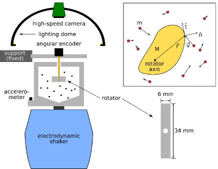
Figure 1: Setup and definition of theoretical quantities.

The granular gas used is made of $N=50$ spheres of polyoxymethylene (diameter $d=$6\text{\,}\mathrm{mm}$$ and mass $m=$0.15\text{\,}\mathrm{g}$$) in a cylinder of volume $V\approx$1.9\text{\times}{10}^{5}\text{\,}\mathrm{m}\mathrm{m}^{3}$$ (and number density $n=N/V$). The cylinder is shaken with a sinusoidal signal at $53\text{\,}\mathrm{Hz}$ and variable amplitude (measured by the maximum rescaled acceleration $a_{\text{max}}/g$ where $g$ is the gravity acceleration). Suspended into the gas, a pawl (also called “rotator”) of total surface $\Sigma=$1.2\text{\times}{10}^{3}\text{\,}\mathrm{m}\mathrm{m}^{2}$$ (height $h=$15\text{\,}\mathrm{mm}$$ and base perimeter $S=\Sigma/h$), mass $M=$6.49\text{\,}\mathrm{g}$$ and momentum of inertia $I=$353\text{\,}\mathrm{g}\,\mathrm{m}\mathrm{m}^{2}$$ rotates around a vertical axis attached to two ball bearings. The position of the rotator is recorded in time by an angular encoder (Avago Technologies). It is convenient to introduce the radius of inertia $R_{I}=\sqrt{I/M}$ of the rotator. See Fig. 1 for a sketch of the system and the definition of some quantities.

A close analysis of the dynamics of the rotator shows that it is well described by the following equation of motion:

$$\dot{\omega}=-\Delta\sigma(\omega)-\gamma_{a}\omega+\eta_{coll}(t)$$ (1)

where $\Delta=F_{frict}/{I}=$38\text{\,}\mathrm{pm}$$4\text{\,}\mathrm{s}^{-2}$$ is the frictional force rescaled by inertia, $\gamma_{a}=$6\text{\,}\mathrm{pm}$$1\text{\,}\mathrm{s}^{-1}$$ is some viscous damping rate related perhaps to air or to other dissipations in the bearings, and $\eta_{coll}(t)$ is the random force due to collisions with the granular gas particles. The granular gas itself is stationary and (roughly) homogeneous.

The velocity distribution of the spheres on the plane perpendicular to the rotation axis is obtained by particle tracking via a fast camera (see [19] for details on the procedure) and is fairly approximated by a Gaussian,

$$\phi(v)\sim e^{-v^{2}/(2v_{0}^{2})},$$ (2)

where the “thermal” velocity $v_{0}$ has been introduced. Small deviations from the Gaussian are observed but are neglected for the purpose of this study; see [20] for details. We have changed the maximum acceleration rescaled by gravity $a_{\text{max}}/g$ from $6$ to $20$, finding for $v_{0}$ values from $200\text{\,}\mathrm{m}\mathrm{m}^{2}\,\mathrm{s}^{-2}$ to $500\text{\,}\mathrm{m}\mathrm{m}^{2}\,\mathrm{s}^{-2}$.

The pawl is further characterized by its symmetric shape factor $\langle g^{2}\rangle_{surf}=1.51$, where $\langle\cdot\rangle_{surf}$ denotes a uniform average over the surface of the object parallel to the rotation axis (see [21] for details). The restitution coefficient between the spheres and the pawl has been measured to be $\alpha\approx 0.83$. It is also useful to introduce the “equipartition” angular velocity $\omega_{0}=v_{0}\epsilon/R_{I}$ where $\epsilon=\sqrt{\frac{m}{M}}$. Note that, because of inelastic collisions and frictional dissipations, the rotator does not satisfy equipartition and $\omega_{0}$ is only a useful reference value.

3 Boltzmann equation

Since the packing fraction of the system does not exceed $3\%$, the single-particle probability density function (pdf) $p(\omega,t)$ of the angular velocity of the rotator is expected to be fully described, under the assumption of diluteness which guarantees molecular chaos, by the following equation [22, 21, 8]:

$$\partial_{t}p(\omega,t) =\partial_{\omega}[(\Delta\sigma(\omega)+\gamma_{a}\omega)p(\omega,t)]+J[p,\phi]$$ (3a)

$$J[p,\phi] =\int d\omega^{\prime}\,W(\omega|\omega^{\prime})p(\omega^{\prime},t)-p(\omega,t)f_{c}(\omega),$$ (3b)

$$W(\omega^{\prime}|\omega) =\rho S\int\frac{ds}{S}\int d{\mathbf{v}}\,\phi({\mathbf{v}})\Theta[({\mathbf{V}}(s)-{\mathbf{v}})\cdot\hat{n}]\times$$ (3c)

$$|({\mathbf{V}}(s)-{\mathbf{v}})\cdot\hat{n}|\delta[\omega^{\prime}-\omega-\Delta\omega(s)],$$

$$\Delta\omega(s) =(1+\alpha)\frac{[{\mathbf{V}}(s)-{\mathbf{v}}]\cdot\hat{n}}{R_{I}}\frac{g(s)\epsilon^{2}}{1+\epsilon^{2}g(s)^{2}},$$ (3d)

where we introduce the rates $W(\omega^{\prime}|\omega)$ for the transition $\omega\to\omega^{\prime}$, the velocity-dependent collision frequency $f_{c}(\omega)=\int d\omega^{\prime}\,W(\omega^{\prime}|\omega)$, the pdf $\phi({\mathbf{v}})$ for the gas particle velocities, and the so-called kinematic constraint in the form of Heaviside step function $\Theta[({\mathbf{V}}-{\mathbf{v}})\cdot\hat{n}]$, which enforces the kinematic condition necessary for impact. We also use the following symbols: $\rho=nh$, ${\mathbf{V}}(s)=\omega\hat{z}\times{\mathbf{r}}(s)$ is the linear velocity of the rotator at the point of impact ${\mathbf{r}}(s)$ parametrized by the curvilinear abscissa $s$ along the outer perimeter of the rotator, $\hat{n}(s)$ is the unit vector perpendicular to the surface at that point, and finally $g(s)={\mathbf{r}}(s)\cdot\hat{t}(s)/{R_{I}}$ with $\hat{t}(s)=\hat{z}\times\hat{n}(s)$, which is the unit vector tangent to the surface at the point of impact. We refer to Fig. 1 for a visual explanation of these symbols. The collision rule is given by Eq. (3d) [21]. Note that in our setup, at homogeneous fluidization, we measure $\rho S\approx$0.31\text{\,}\mathrm{m}\mathrm{m}^{-1}$$.

4 Different regimes

An important parameter is

$$\beta^{-1}=\frac{\epsilon n\Sigma v_{0}^{2}}{\sqrt{2}\pi R_{I}\Delta}\approx\frac{\tau_{\Delta}}{\tau_{c}},$$ (4)

which estimates the ratio between the stopping time $\tau_{\Delta}\sim\omega_{0}/{\Delta}$ due to dissipation (dominated by dry friction) and the collisional time $\tau_{c}\sim{(n\Sigma v_{0})}^{-1}$. A transition at $\beta\sim 1$ is expected between a regime called the rare collision limit (RCL) at $\beta^{-1}\ll 1$, with the rotator at rest most of the time, and a regime called the frequent collision limit (FCL) at $\beta^{-1}\gg 1$, with the rotator always in motion, continuously perturbed by collisions. The difference between these two regimes is illustrated in Fig. 2a.

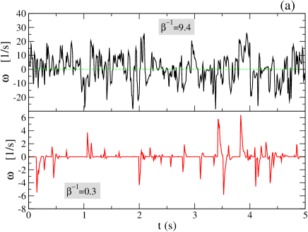
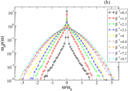
Figure 2: (a) Two examples of signal $\omega(t)$ for different values of $\beta^{-1}$ in the experiment, corresponding to choices of the rescaled maximum acceleration $a_{\text{max}}/g=4.1$ and $20.5$ respectively; (b) rescaled experimental pdfs of the angular velocity for a range of rescaled accelerations going from $4.1$ to $21.2$. All other parameters are in the main text.

The pdfs of the angular velocity obtained experimentally for values of $\beta^{-1}$ spanning the RCL and FCL are reported in Fig. 2b. There is a great variability when $\beta^{-1}$ goes from small to large values, i.e., when increasing the shaking amplitude and, consequently, the collision frequency. At large values of $\beta^{-1}$, the pdfs rescaled by $\omega_{0}$ tends to superimpose, a sign that $\omega_{0}$ becomes the leading velocity scale. In order to make a more detailed contact with the theory and understand the basic properties of the velocity pdf, we discuss next the RCL and FCL regimes separately.

5 Rare collision limit

As seen above, the pawl in the RCL ($\beta^{-1}\ll 1$) is often at rest, resulting in a peak around $\omega=0$ in the angular velocity pdf. To describe this peak, we approximate the expected stationary pdf as

$$p(\omega)=a\delta(\omega)+(1-a)p_{smooth}(\omega),$$ (5)

where $a$ is a suitable weight, decreasing as $\beta^{-1}$ grows, and $p_{smooth}(\omega)$ represents the smooth part of the pdf.

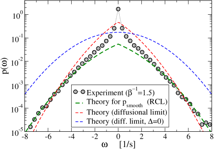
Figure 3: Pdf of the pawl’s angular velocity in the rare collisions limit (RCL), obtained with a maximum rescaled acceleration of the shaker given by $a_{\text{max}}/g=6.5$ ($\beta^{-1}=1.5$). All other parameters of the experiment are given in the main text. The theoretical prediction (7) is displayed as the dashed green line, where only $a$ is fitted with the experimental data. For reference, we also show the prediction of the theory in the diffusive limit with and without dry friction as the dashed red and blue curves, respectively.

This form of stationary pdf has been studied in [8, 17, 23]. In the RCL, the dynamics is reduced to independent collisions followed by friction-induced relaxations. More precisely, at a collision time $t$ the rotator velocity changes from $0$ to $\omega^{*}$, depending on the projected impact velocity $v=\mathbf{v}\cdot\hat{n}$ and the projected impact point $g=\mathbf{r}\cdot\hat{t}/R_{I}$, and then relaxes according to $\dot{\omega}=-\Delta\sigma(\omega^{*})$ until a time $t+\tau$ such that $\omega(t+\tau)=0$. In this case, the stationary average of any function $y(\omega)$, restricted to the times where $\omega(t)\neq 0$, can be written as

$$\langle y\rangle=\rho S\int\frac{dS}{S}\int_{-\infty}^{0}dv\,|v|\phi(v)\int_{0}^{\tau}dt\,y[\omega(t)].$$ (6)

With this formula, we can calculate the characteristic function of $\omega$ by taking $y=e^{ik\omega}$ and then invert the transform to retrieve the smooth part $p_{smooth}(\omega)$. For the Gaussian $\phi(v)$ of variance $v_{0}^{2}$ and the particular shape of our rotator, this yields

$$p_{smooth}(\omega) = \mathcal{N}^{\prime}h\left(\frac{\omega}{(1+\alpha)\omega_{0}}\right),$$ (7)

$$h(x) = \frac{e^{-2x^{2}}}{4|x|}\left\{2-\textrm{erfc}\left[\frac{(\xi-1)|x|}{\sqrt{2\xi}}\right]\right.-$$ (8)

$$\quad\ \left.e^{2x^{2}}\textrm{erfc}\left[\frac{(\xi+1)|x|}{\sqrt{2\xi}}\right]\right\}$$

$$\mathcal{N}^{\prime} = \left[\int d\omega h\left(\frac{\omega}{(1+\alpha)\omega_{0}}\right)\right]^{-1}.$$ (9)

This result is compared with our experimental data in Fig. 3. It can be seen that the agreement of the tail is very good, considering that we only fit the overall scaling factor $a$ representing the weight relative to the $\delta(\omega)$ contribution. On the contrary, the central part is not well reproduced. We suspect that the discrepancy at low velocities is due to a failure of the Coulomb friction model at those regimes. A close inspection of single trajectories indeed reveals that the free relaxing rotator frequently comes to rest with spurious oscillations, likely to be due to the ball dynamics inside the bearings. This observation points to an interesting application of studying ball bearings under random excitation: in our case, the macroscopic observation of $p(\omega)$ magnifies microscopic features around the zero velocity which would be hard to characterize and understand otherwise.

From the experiment, we can also evaluate the autocorrelation $C(t)=\langle\omega(t)\omega(0)\rangle$ and power spectrum,

$$S(f)=\left|\sum_{j}\omega(t_{j})e^{2\pi\sqrt{-1}ft_{j}}\right|^{2}.$$ (10)

These are shown in Fig. 5 as red curves. To our knowledge, no theory is available for these quantities in the RCL. We notice that the large frequency decay of the spectrum $S(f)\sim f^{-2}$ is compatible with a small time exponential decay, while the part at small $f$ deviates from it, suggesting a more rapid decay at large times. These features are recovered in the graph of $C(t)$. Note that the power spectrum also shows one of the higher harmonics of the shaker frequency ($3\times 53=$159\text{\,}\mathrm{Hz}$$): it emerges only when the main signal due to the dynamics of the rotator under the collisions becomes weak enough and disappears in the FCL where the energy injected by the collisions is larger.

6 Frequent collisions and large rotator mass: equivalence with continuous white noise

In the FCL, it is useful to exploit the difference of mass (here $\epsilon=\sqrt{m/M}=0.15$) by taking a further $\epsilon\ll 1$ limit. Such a limit is often called a “diffusive limit” and allows us to expand the Boltzmann equation (3) to obtain a Fokker-Planck equation or, equivalently, a Langevin equation for the pawl velocity [21] having the form

$$\dot{\omega}=-\gamma\omega-\Delta\sigma(\omega)+\sqrt{\Gamma_{g}}\,\xi,$$ (11)

where $\gamma=\gamma_{a}+\gamma_{g}$, $\gamma_{g}$ represents a granular viscosity, $\gamma_{a}$ an air viscosity, $\Gamma_{g}$ a granular velocity diffusion coefficient, and $\xi$ is a Gaussian white noise with unit variance. In our setting, $\gamma_{g}$ and $\Gamma_{g}$ are given by [21]

$$\gamma_{g} =(1+\alpha)\sqrt{\frac{2}{\pi}}\rho S\frac{m}{M}v_{0}\langle g^{2}\rangle_{surf}$$ (12a)

$$\Gamma_{g} =(1+\alpha)\gamma_{g}\frac{m}{I}v_{0}^{2}.$$ (12b)

The study of the Langevin equation (11) was initiated in [1], received strong impulse by de Gennes in [12], and was completed in [13, 14, 15, 16]. Its stationary velocity distribution reads [24]

$$p(\omega) =\mathcal{N}\exp\left[-\frac{(|\omega|+\Delta/\gamma)^{2}}{\Gamma_{g}/\gamma}\right],$$ (13)

$$\mathcal{N}^{-1} =\sqrt{\pi\Gamma_{g}/\gamma}\;\textrm{erfc}(\Delta/\sqrt{\gamma\Gamma_{g}}).$$ (14)

Note that in the limit $\beta\to 0$, e.g., when dry friction disappears ($\Delta\to 0$), the stationary pdf goes to a Gaussian of variance $\Gamma_{g}/\gamma$. Moreover, assuming also $\gamma_{a}\ll\gamma_{g}$ (which is consistent with the FCL), one has $\Gamma_{g}/\gamma\approx\omega_{0}^{2}(1+\alpha)/{2}$, so that equipartition with the gas $\langle\omega^{2}\rangle=\omega_{0}^{2}$ is satisfied in the ideal elastic case $\alpha=1$ [25].

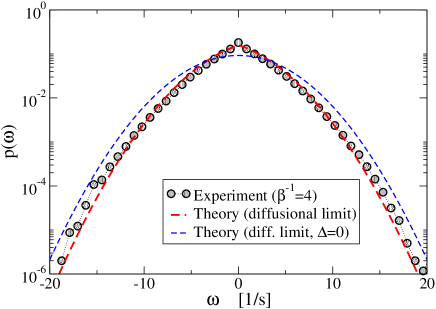
Figure 4: Pdf of the pawl’s angular velocity in the frequent collisions regime (FCL) obtained when the maximum rescaled acceleration of the shaker is $a_{\text{max}}/g=11.74$. The prediction of the diffusive limit theory, Eq. (13), is displayed as the dashed red line with no fitting parameters. For reference, we also show with the dashed blue line the prediction of the diffusive limit without dry friction.

In Fig. 4, we find good agreement between the pdf above and the experimental data. This comparison, obtained with no fitting parameters, represents one of the first known experimental verification of the velocity pdf (13), as well as one of the few experimental applications of the diffusive limit of granular kinetic theory. The cusp at $\omega=0$ predicted by the theory is a striking consequence of the presence of Coulomb friction, and is well reproduced in the experimental data. At large velocities, $\omega\gg\Delta/\gamma\approx$6\text{\,}\mathrm{s}^{-1}$$, the pdf recovers Gaussian tails due to the dominance of linear viscosity.

In the diffusive limit, where Eq. (11) holds, theoretical expectations for the autocorrelation of the angular velocity and for the power spectrum have been obtained analytically in [13, 16]. These expressions involve the eigenvalues of the Fokker-Planck operator, and are too long to be reproduced here. A verification of these expressions, shown in Fig. 5, indicates that the Langevin model of Eq. (11) offers a good description of our experiment in the FCL.

7 Relevance of friction in the FCL

A more refined comparison of experiment and theory is obtained in Fig. 6, where three main observables are plotted against $\beta^{-1}$: the rescaled peak of the velocity distribution, the variance of the distribution, and the correlation time $\tau_{c}$ obtained by fitting $C(t)\sim\exp(-t/\tau_{c})$. The three figures also show the predictions, for each choice of the parameters, of the diffusive limit theory, as given by Eq. (11), together with the predictions of the same theory in the absence of dry friction ($\Delta=0$). This last comparison is useful to evaluate the relevance of the dry friction term.

In Fig. 6a, we display the peak of the experimental pdf (again rescaled by $\omega_{0}$) as a function of $\beta^{-1}$. This information, in the RCL when the rotator is most of the time at rest, is an indirect probe of $a$, since the experimental value $p(0)$ includes also $(1-a)p_{smooth}(0)$. This figure clearly shows the decrease of the peak as $\beta^{-1}$ increases. Moreover, it shows that, when $\beta^{-1}>1$, such a peak gets closer to the values analytically computed in the diffusive limit where $\Delta$ is negligible and the pdf tends to a Gaussian. Interestingly, the variance of the distribution $\langle\omega^{2}\rangle$, whose formula in the diffusive limit reads

$$\langle\omega^{2}\rangle=\left(\frac{\Delta}{\gamma}\right)^{2}+\frac{\Gamma_{g}}{2\gamma}-\mathcal{N}\frac{\Delta\Gamma_{g}}{\gamma^{2}}\exp\left(-\frac{\Delta^{2}}{\gamma\Gamma_{g}}\right),$$ (15)

adheres to the prediction of the diffusive theory even in the RCL, while at large $\beta^{-1}$ both the experiment and the diffusive theory go toward the linear limit, where $\Delta$ is negligible. The small discrepancies are likely to be due to the finiteness of the mass ratio $\epsilon$ in the experiment.

A different scenario is observed for the correlation time $\tau_{c}$, as the experiment shows a non-monotonous behavior when plotted against $\beta^{-1}$, with $\tau_{c}$ growing when moving from the RCL to the FCL, up to a regime where the experiment is well described by the diffusive theory (red line). This regime displays a slight decrease of $\tau_{c}$ as $\beta^{-1}$ is further increased. It is interesting to note that, even at the highest values of $\beta^{-1}$, the prediction of the linear theory without friction ($\Delta=0$) overestimates by roughly $40\%$ the experimental results. The correlation time is therefore very sensitive to the presence of the dry friction and signals it even when the “static” information coming from the velocity pdf is basically not affected.

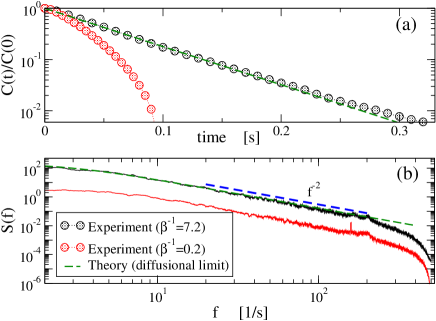
Figure 5: (a) Autocorrelation and (b) power spectrum of the pawl’s angular velocity in the FCL (black) and RCL (red) obtained with a maximum rescaled acceleration of the shaker corresponding to $a_{\text{max}}/g=4.1$ and $17$, respectively. The diffusive limit prediction is superimposed as the dashed green line.

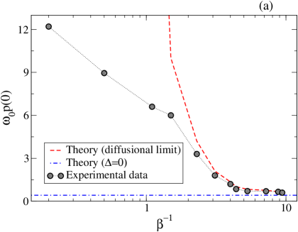
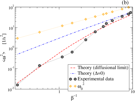
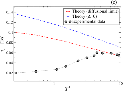
Figure 6: Comparison of experiments (black points) versus theory in the diffusive limit with dry friction (red lines) and without dry friction (blue lines), in order to evaluate the relevance of friction as $\beta^{-1}$ is varied: (a) rescaled peak of the velocity pdf; (b) variance of the velocity pdf; (c) decay time of the velocity autocorrelation.

8 Conclusions

We have discussed in this letter the results of an experiment in which a rotator is submitted to dry friction and collisions with a granular gas. By tuning the shaking amplitude at constant frequency, we have explored different random, Brownian-like dynamics which are either dominated by friction or by collisions, as well as the crossover between these two extreme regimes. In the rare collision regime (RCL), our data for the velocity pdf display a macroscopic fraction of events at rest ($\omega=0$) and non-Gaussian tails at high velocity, which are both well reproduced by a Boltzmann collision model. In the frequent collision regime (FCL), our results for the velocity pdf, autocorrelation and power spectrum are well explained by a Langevin model with dry and viscous frictions [13], which can be derived from the Boltzmann model in the diffusive limit. In this limit, dry friction tends to become negligible compared to the other forces; this explains why, at very high collision frequency, one recovers a phenomenology partly explained by the Ornstein-Uhlenbeck model, if we exclude the correlation decay.

To conclude, we remark that our experiment suggests a useful way to estimate parameters which are somewhat difficult to measure directly, in analogy with Einstein’s theory of Brownian motion which gives access to Avogadro’s number through a macroscopic measurement. In our case, Eq. (15) together with the expressions shown in (12) may be used to obtain estimates of $\alpha$ or $\Delta$ knowing the other parameters and the value of $\langle\omega^{2}\rangle$. At the same time, our experiment offers a positive test of the ability of kinetic theory to predict macroscopic Brownian coefficients, such as the viscosity $\gamma_{g}$ and the noise amplitude $\Gamma_{g}$. Ongoing extensions of our study include the coupling of the system with a motor [26] in order to apply an external force and investigate its interplay with friction and collisions [13], and the possibility of observing ratchet effects for asymmetric rotators [8, 27, 20].

- [1] T. K. Caughey and J. K. Dienes. Analysis of a nonlinear first‐order system with a white noise input. J. Appl. Phys., 32:2476, 1961.
- [2] J. D. Atkinson and T. K. Caughey. First order piecewise linear systems with random parametric excitation. Int. J. Non-Linear Mech., 3:399–411, 1968.
- [3] J. D. Atkinson and T. K. Caughey. Spectral density of piecewise linear first order systems excited by white noise. Int. J. Non-Linear Mech., 3:137–156, 1968.
- [4] E. Riedo and E. Gnecco. Thermally activated effects in nanofriction. Nanotechnology, 15:S288, 2004.
- [5] M. Eglin, M. A. Eriksson, and R. W. Carpick. Microparticle manipulation using inertial forces. Appl. Phys. Lett., 88:091913, 2006.
- [6] A. Buguin, F. Brochard, and P.-G. de Gennes. Motions induced by asymmetric vibrations. Eur. Phys. J. E, 19:31–36, 2006.
- [7] D. Fleishman, Y. Asscher, and M. Urbakh. Directed transport induced by asymmetric surface vibrations: making use of friction. J. Phys.: Condens. Matter, 19:096004, 2007.
- [8] J. Talbot, R. D. Wildman, and P. Viot. Kinetic of a frictional granular motor. Phys. Rev. Lett., 107:138001, 2011.
- [9] S. Daniel, M. K. Chaudhury, and P.-G. de Gennes. Vibration-actuated drop motion on surfaces for batch microfluidic processes. Langmuir, 21:4240, 2005.
- [10] S. Mettu and M. K. Chaudhury. Stochastic relaxation of the contact line of a water drop on a solid substrate subjected to white noise vibration: Roles of hysteresis. Langmuir, 26:8131, 2010.
- [11] P. S. Goohpattader and M. K. Chaudhury. Diffusive motion with nonlinear friction: apparently brownian. J. Chem. Phys., 133:024702, 2010.
- [12] P.-G. de Gennes. Brownian motion with dry friction. J. Stat. Phys., 119:953, 2005.
- [13] H. Touchette, E. Van der Straeten, and W. Just. Brownian motion with dry friction: Fokker-Planck approach. J. Phys. A: Math. Theor., 43:445002, 2010.
- [14] A. Baule, E. G. D. Cohen, and H. Touchette. A path integral approach to random motion with nonlinear friction. J. Phys. A: Math. Theor., 43:025003, 2010.
- [15] A. Baule, H. Touchette, and E. G. D. Cohen. Stick-slip motion of solids with dry friction subject to random vibrations and an external field. Nonlinearity, 24:351, 2011.
- [16] H. Touchette, T. Prellberg, and W. Just. Exact power spectra of brownian motion with solid friction. J. Phys. A: Math. Theor., 45:395002, 2012.
- [17] A. Baule and P. Sollich. Singular features in noise-induced transport with dry friction. EPL, 97:20001, 2012.
- [18] T. Pöschel and S. Luding, editors. Granular Gases, Berlin, 2001. Springer. Lecture Notes in Physics 564.
- [19] A. Puglisi, A. Gnoli, G. Gradenigo, A. Sarracino, and D. Villamaina. Structure factors in granular experiments with homogeneous fluidization. J. Chem. Phys., 136:014704, 2012.
- [20] A. Gnoli, A. Petri, F. Dalton, G. Gradenigo, G. Pontuale, A. Sarracino, and A. Puglisi. Brownian ratchet driven by Coulomb friction. Phys. Rev. Lett., 110:120601, 2013.
- [21] B. Cleuren and R. Eichhorn. Dynamical properties of granular rotors. J. Stat. Mech., P10011, 2008.
- [22] N. G. van Kampen. A power series expansion of the master equation. Can. J. Phys., 39:551, 1961.
- [23] A. Baule and P. Sollich. Rectification of asymmetric surface vibrations with dry friction: An exactly solvable model. Phys. Rev. E, 87:032112, 2013.
- [24] H. Hayakawa. Langevin equation with Coulomb friction. Physica D, 205:48, 2005.
- [25] A. Sarracino, D. Villamaina, G. Costantini, and A. Puglisi. Granular brownian motion. J. Stat. Mech., P04013, 2010.
- [26] A. Naert. Experimental study of work exchange with a granular gas: The viewpoint of the fluctuation theorem. EPL, 97:20010, 2012.
- [27] S. Joubaud, D. Lohse, and D. Van Der Meer. Fluctuation theorems for an asymmetric rotor in a granular gas. Phys. Rev. Lett., 108:210604, 2012.