Realistic polarizing Sagnac topology with DC readout for the Einstein Telescope

Abstract

The Einstein Telescope (ET) is a proposed future gravitational wave detector. Its design is original, using a triangular orientation of three detectors and a xylophone configuration, splitting each detector into one high-frequency and one low-frequency system. In other aspects the current design retains the dual-recycled Michelson interferometer typical of current detectors, such as Advanced LIGO. In this paper, we investigate the feasibility of replacing the low-frequency part of the ET detectors with a Sagnac interferometer. We show that a Sagnac interferometer, using realistic optical parameters based on the ET design, could provide a similar level of radiation pressure noise suppression without the need for a signal recycling mirror and the extensive filter cavities. We consider the practical issues of a realistic, power-recycled Sagnac, using linear arm cavities and polarizing optics. In particular, we investigate the effects of nonperfect polarizing optics and propose a new method for the generation of a local oscillator field similar to the DC readout scheme of current detectors.

I Introduction

The Einstein gravitational-wave Telescope (ET) is a proposed third-generation gravitational wave (GW) observatory. Its aim is to achieve a factor of 10 improvement in sensitivity with respect to the advanced detectors, such as Advanced LIGO Harry and the LIGO Scientific Collaboration (2010) and Advanced VIRGO  Accadia et al. (2011), over a broad range of frequencies Sathyaprakash et al. (2012). The current design of ET is based on three nested detectors, each being composed of two Michelson interferometers (xylophone design Shoemaker (2001); Hild et al. (2010)), one optimized for low frequencies (ET-LF) and the other for high frequencies (ET-HF). Both interferometers have 10 km long arm cavities and use a dual-recycled Michelson configuration (combining power recycling and signal recycling). The xylophone design has been proposed to optimize the sensitivity between 2-40 Hz and 40 Hz-10 kHz independently, allowing the separation of cryogenic optics from high power laser beams. ET-HF is mainly concerned with the photon counting noise (shot noise) and employs high laser power. ET-LF was designed particularly to minimize the low-frequency quantum noise caused by quantum fluctuations of the photon number (radiation pressure noise) by using a low optical power. ET has been envisaged as an infrastructure that could host different implementations of GW detectors over a long time and therefore the design offers the flexibility to choose different topologies and configurations other than the dual-recycled Michelson interferometer.

Initial proposals for interferometric measurements for GW detection favored the Michelson interferometer because it naturally provides a differential length measurement between perpendicular arms. This maximizes the signal for a GW (of one polarization and direction) so is ideally suited for GW detection. The original purpose of the Sagnac interferometer was to measure rotation rather than mirror displacement Sagnac (1913). In 1995, successful experimental tests of a zero-area Sagnac demonstrated a different mode of operation, in which it becomes insensitive to rotation but sensitive to mirror motion Sun et al. (1996). The zero-area Sagnac interferometer was thus revealed as an alternative approach with the potential of reaching the required sensitivity to detect GWs. Further investigations into the performance and technical limitations of a Sagnac interferometric GW detector has been developed Petrovichev et al. (1998); Beyersdorf et al. (1999a, b). A reduced susceptibility to laser frequency fluctuations and imbalances of mirror positions was identified Petrovichev et al. (1998) and experimentally verified with a heterodyne detection Beyersdorf et al. (1999a). However, this comes at the cost of tighter tolerances of the imperfections (i.e., mirror surface distortions) and misalignments (i.e., beam splitter tilt, mirror tilt) of optical components compared to the Michelson topology Petrovichev et al. (1998); Beyersdorf et al. (1999b). The use of a Sagnac also implies challenges in the length control of the combination of arm cavities and dual-recycling mirrors Mizuno et al. (1997). These drawbacks along with the rapid development of advanced techniques for the further enhancement of the Michelson performance previously prevented a more serious consideration of the Sagnac topology for GW detection.

After significant efforts in reducing classical noise sources in the GW community Harry and the LIGO Scientific Collaboration (2010), the impact of quantum noise is now one of the most important challenges in designing future GW observatories, in particular the Einstein Telescope Abernathy et al. (2011a). To reduce the quantum noise over a broad frequency band, the baseline of the current ET design includes the injection of frequency-dependent squeezed vacuum into the dark port of both the LF and HF Michelson interferometers. The frequency-dependent rotation of the squeezing angle is facilitated by implementing two long filter cavities for each interferometer Abernathy et al. (2011a). Alternatively, in 2003 Chen Chen (2003) first described the quantum-nondemolition properties of a Sagnac-type interferometer as it functions as a speed meter rather than a position meter, which can remove the low-frequency radiation pressure noise without the need of two long filter cavities. A comprehensive quantum noise analysis of a practical large-scale Sagnac interferometer (using LIGO parameters) has been carried out Chen (2003); Danilishin (2004), including the consideration of optical losses. In Chen (2003), the application of km-scale ring cavity and delay line schemes in a Sagnac interferometer has been investigated. The studies revealed very promising quantum noise characteristics at low frequencies (1 Hz - 100 Hz) with only little susceptibility to optical losses. A variant scheme is shown in  Danilishin (2004); Chen et al. (2011); Danilishin and Khalili (2012) with minimal changes to current existing detector configurations by using polarizing optical components (polarization speed meter based on Michelson configuration has recently been investigated by Wade et al. Wade et al. (2012)). It has been shown that such a configuration using squeezed vacuum injection but without filter cavities can reduce low-frequency quantum noise to a similarly low level as a Michelson with filter cavities Danilishin and Khalili (2012). Recently, a tabletop experiment has demonstrated quantum noise reduction by nonfiltered squeezing in a Sagnac interferometer Eberle et al. (2010).

During the ET design study the Sagnac topology was investigated as an alternative option for the low-frequency part of the xylophone (ET-LF)  Müller-Ebhard et al. (2009), focusing on a Sagnac design with ring cavities in the interferometer arms. However, ring cavities with a long baseline imply a number of challenges, such as elliptical spot sizes on some mirrors and a larger coupling of small-angle scattering back into the main beam. Because of the vast experience using a Michelson interferometer within the GW community and the advancements in technology specifically based on the Michelson, a Sagnac topology was not chosen for the original ET design.

In this paper, we reconsider the Sagnac topology for the realization of the ET-LF interferometers. Precisely, we compare the originally proposed Michelson-type interferometer with two auxiliary filter cavities to a Sagnac-type interferometer without filter cavities. The latter promises a significant reduction of complexity and cost for the construction of the ET observatory whilst achieving a compelling quantum-noise limited sensitivity. In contrast to earlier considerations that investigated interferometers with ring cavities, we study the Sagnac configuration with polarizing optical components and linear Fabry-Pérot arm cavities. Technical concerns of this configuration including the influence of realistic polarizing optics on the dark fringe output and the null response of a Sagnac to static mirror displacement are solved in an elegant way. We describe a novel method for using the leakage due to the polarizers’ finite extinction ratio to create a Local Oscillator (LO) for an optical readout scheme similar to the DC readout adopted by advanced GW detectors adl (2007); Ward et al. (2008); Hild et al. (2009); Fricke et al. (2012). This has, to the best of our knowledge, never been considered before. We analyze the quantum noise behavior of a realistic ET-LF Sagnac instrument with imperfect polarizing optics and frequency-independent squeezing. With only minor adjustments on the ET-LF parameters, we show that a comparable quantum noise level is feasible without the use of filter cavities and also the signal recycling mirror.

The paper is organized as follows: Section II discusses different practical realizations of a polarizing Sagnac interferometer with linear arm cavities. One realization is selected for this study and justified. In Sec. III, we compute the quantum noise of the selected polarizing Sagnac interferometer with ET-LF parameters. For simplicity, we start with the case of perfect polarizing optics and illustrate the input-output relation by using block diagrams. Since we propose to use a slightly increased laser power, adjustments of the mirror thermal noise and the effect on the overall noise level are discussed briefly. We do not attempt to propose a full alternative design for ET. However, we present a discussion on the noise projection for a Sagnac-type design targeting a comparable quantum noise budget as the planned ET-LF Michelson. Simple scaling laws are applied to the other noise sources. We then extend our quantum noise model by considering a finite extinction ratio to account for realistic polarizing beam splitters. The quantum noise level is evaluated for different degrees of imperfections and varying parameters of the leakage-enabled DC readout scheme before a sensitivity comparison between a Sagnac and the current ET-LF design is presented. Requirements and different approaches for creating a practical LO for a DC readout scheme are discussed in more detail in Sec. IV. We also investigate different approaches to select a homodyne detection angle and present a novel method to correctly choose it. In the end of the section, we model the polarizing Sagnac interferometer using Finesse Freise et al. (2004); Freise and show the possibilities to control different degrees of freedom (DoFs). In Sec. V we give a comprehensive conclusion of our findings.

II Polarizing Sagnac Interferometer

Figure 1: Two versions of a polarizing Sagnac interferometer configuration. Both require minimum changes to the current ET-LF Michelson interferometers; relevant parameters are summarized in Table 1. The interferometer has two linear Fabry-Pérot arm cavities with a length of 10 km. A PBS transmits p-polarized and reflects s-polarized light. A QWP transforms the linearly polarized beam into a circularly polarized beam and vice versa with a rotated 90^∘ angle relative to the initial linear polarization. The left configuration which specifies each light field (i.e., a, b, etc) will be used to evaluate the input-output relation in Sec. III.1. The arrows denote the p-polarized (blue) and s-polarized (green) beams which are respectively totally transmitted and reflected by an ideal PBS. Light fields circulating inside both arm cavities are circularly polarized (black) beams with both direction rotations.

Parameter	Michelson	Sagnac
Arm length	10 km	10 km
Distance PRM-BS	10 m	10 m
Distance BS-ITM	300  m	300 m
Distance BS-PBS	…	10 m
Distance PBS-QWP	…	10 m
Distance QWP-ITM	…	280 m

Table 1: A table summarizing the baseline parameters of the ET-LF Michelson interferometer and an alternative Sagnac interferometer. The Michelson values are taken from the original design study report Abernathy et al. (2011a). The Sagnac values are suggested by us for an ET Sagnac layout.

A realization of a Sagnac interferometer with minimum changes to the planned ET infrastructure can be achieved by adding polarizing beam splitters (PBSs) and quarter-wave plates (QWPs) to the current layout. Two possible polarizing Sagnac configurations are shown in Fig. 1. They differ from a Michelson interferometer as each beam after the central beam splitter (BS) travels through both arm cavities one after another. The two beams share the same optical path but with opposite propagation directions. This is achieved using PBSs and QWPs. The PBSs only transmit the p-polarized beam and reflect the s-polarized. The QWPs transform the linearly polarized beam into a circularly polarized beam and again transform the circularly polarized beam into linear polarization, rotated by 90^∘ relative to the initial linear polarization. Assuming ideal and lossless optical components, configurations (i) and (ii) in Fig. 1 have the same performance in terms of quantum noise reduction. However, in reality each component will add optical losses and complexity. The major difference between configuration (i) and (ii) is the number and position of the PBSs. Configuration (i) has already been selected in previous investigations for a polarizing Sagnac interferometer Danilishin (2004); Chen et al. (2011); Danilishin and Khalili (2012). An ET Sagnac topology baseline is given and the parameters with minimal and reasonable changes to the current Michelson baseline are summarized in Table 1. For the following discussion we have picked configuration (i) which features only one PBS and is thus expected to exhibit lower optical losses due to finite extinction ratio.

III Quantum noise of a Sagnac Interferometer

We analyze the quantum noise behavior of a polarizing Sagnac interferometer as shown in Fig. 1 (i), taking into account the imperfect nature of a realistic PBS. To get the quantum noise spectral density (NSD), the input-output relation of the interferometer needs to be specified Kimble et al. (2001). Throughout this paper we present the input-output relations using intuitive block diagrams. We first consider the case of an ideal PBS (Sec. III.1) and then extend the model to include the effects of an imperfect PBS (Sec. III.2). In this paper, we only consider the imperfection that a PBS has finite extinction ratio which induces a mixing of the two polarized fields. Optical losses from arm cavities have been included and investigated for both cases. We compare the quantum noise for the same setup using PBSs with different extinction ratios and propose an approach to increase the signal to noise ratio of such a realistic Sagnac setup by using an additional PBS at the detection port (to reduce the mixing of two polarized fields).

III.1 Polarizing Sagnac interferometer with perfect PBS

For the implementation of the block diagram concept, the Sagnac interferometer [see Fig. 1 (i)] is split into several principal parts as shown by the blocks in Fig. 2. Each block is defined by its transfer function (TF), where ${\bf M}_{\rm arm}$ is the TF of arm cavity, ${\bf M}_{\rm h}$ is the GW signal TF and ${\bf M}_{\rm n}$ is noise TF which is induced by optical losses.

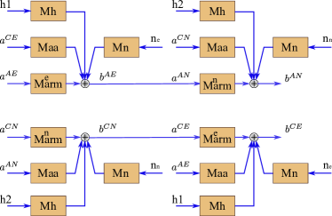
Figure 2: Block diagrams of a polarizing Sagnac interferometer. Each light field corresponds to that has shown in Fig. 1 (i) and each block follows the definition in Appendix A. The mechanical displacements $x_{1,2}$ due to the radiation pressure force of the light circulating in the cavities, occur only at the end mirrors. Any light transmitted by the end mirror (EM) is considered as an optical loss. For a lossless cavity, $R_{e}=1$, $T_{e}=0$. QWPs are assumed to be perfect for polarization rotation. Please note that ${\bf M}_{\rm arm}^{n}$ is exactly the same as ${\bf M}_{\rm arm}^{e}$; the different subscripts simply indicate which light field enters which arm first.

All the blocks used here are derived in Appendix A. Following the propagation path of the vacuum field through the Sagnac interferometer we can represent the input-output relation. More specifically, we can derive the propagation relation between $g$ and $q$ [see Fig. 1 (i)] in terms of optical losses (all the fields shown in the block diagrams have been denoted correspondingly in the schematic). Following the two signal flows in Fig. 2, we obtain

$$b^{CE}-b^{AN}=\; {\bf M}_{\rm arm}(a^{CE}-a^{AN})+{\bf M}_{\rm aa}(a^{AE}-a^{CN})$$

$$+{\bf M}_{\rm h}(h_{1}-h_{2})+{\bf M}_{\rm n}(n_{e}-n_{n}),$$ (1)

$$a^{CE}-a^{AN}=\; b^{CN}-b^{AE}$$

$$=\; {\bf M}_{\rm arm}(a^{CN}-a^{AE})-{\bf M}_{\rm aa}(a^{CE}-a^{AN})$$

$$-{\bf M}_{\rm h}(h_{1}-h_{2})-{\bf M}_{\rm n}(n_{e}-n_{n}),$$ (2)

where ${\bf M}_{\rm arm}$, ${\bf M}_{\rm h}$, and ${\bf M}_{\rm n}$ are defined in Eqs. (101) and (102), and

$${\bf M}_{\rm aa}=e^{2i\phi_{arm}}\left[\begin{array}[]{cc}0&0\\ -\kappa_{arm}&0\end{array}\right]$$ (3)

is induced by the two polarized fields circulating inside the arm cavities. Combining the junction equations of light fields $g,q$, dimensionless GW strain $h$ and additional optical losses induced quadrature $n$ at the central BS

$$g=\frac{a^{AE}-a^{CN}}{\sqrt{2}},\qquad q=\frac{b^{CE}-b^{AN}}{\sqrt{2}},$$ (4)

$$h=h_{1}-h_{2},\qquad\quad\;\;\,n=\frac{n_{e}-n_{n}}{\sqrt{2}},$$ (5)

the input-output relation of a Sagnac interferometer with a perfect PBS and optical losses in the arm cavities is

$$q={\bf M}_{\rm sag}g+{\bf H}_{\rm sag}h+{\bf N}_{\rm sag}n,$$ (6)

where

$${\bf M}_{\rm sag}=e^{2i\phi_{sag}}\left[\begin{array}[]{cc}1&0\\ -\kappa_{sag}&1\end{array}\right],\qquad{\bf H}_{\rm sag}=e^{i\phi_{sag}}\frac{\sqrt{2\kappa_{sag}}}{h_{SQL}}\left[\begin{array}[]{c}0\\ 1\end{array}\right]$$ (11)

$${\bf N}_{\rm sag}=e^{i\phi_{sag}}\sqrt{T_{e}}\sqrt{\frac{\kappa_{sag}}{\kappa}}\left[\begin{array}[]{cc}1&0\\ N&1\end{array}\right],$$ (14)

$$N=e^{2i\phi_{arm}}\kappa_{arm}-e^{i\phi_{arm}-i\Omega\tau}\sqrt{\frac{\kappa\kappa_{arm}}{T_{i}}}\,.$$ (15)

The corresponding parameters, which follow the same definitions as in Chen (2003), are

$$\kappa_{arm}=\frac{T_{i}\kappa}{1-2\sqrt{R_{i}}\cos(2\Omega\tau)+R_{i}},\qquad h_{SQL}=\sqrt{\frac{8\hbar}{m\Omega^{2}L^{2}}},$$

$$\phi_{arm}=\arctan{\left(\frac{1+\sqrt{R_{i}}}{1-\sqrt{R_{i}}}\tan{\Omega\tau}\right)},\quad\kappa=\frac{8I_{c}\omega_{0}}{mc^{2}\Omega^{2}},\quad\tau=\frac{L}{c},$$

$$\phi_{sag}=2\phi_{arm}+\frac{\pi}{2},\qquad\kappa_{sag}=4\kappa_{arm}\sin^{2}\phi_{arm},$$ (16)

where $h_{SQL}$ is the standard quantum limit (SQL), $R_{i}$ and $T_{i}$ are the reflectivity and transmissivity of the arm cavity input mirror, $I_{c}$ is the circulating power inside the arm cavities, $L$ is the length of arm cavities, $\omega_{0}$ is the laser frequency, $\Omega$ is the GW signal angular frequency, and $m$ is the reduced mass of the test masses. We have included the full equations for both lossless and lossy cavities in Appendix A.

With the relation between $g$ and $q$ [Eq. (6)], we can substitute the Sagnac interferometer matrices and signal recycling (SR) mirror parameters into Eq. (63) to get the full input-output relations ($g^{sr}$ and $q^{sr}$) of a perfect Sagnac interferometer with SR in agreement with Chen (2003). The ET xylophone design allows an independent parameter optimization of the high frequency sensitivity. The SR mirror, which helps to improve and optimize the quantum noise of a Sagnac interferometer at high frequencies at the cost of low-frequency sensitivity, in the ET-LF case is no longer necessary. A setup without signal recycling will reduce the complexity for the control systems significantly. Therefore in the rest of the paper we discuss a setup without signal recycling as shown in Fig. 5.

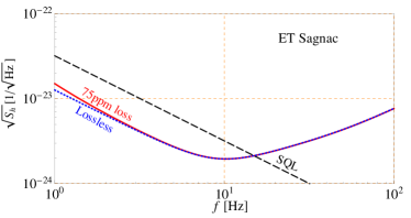
Figure 3: Plots showing the quantum NSD of a polarizing Sagnac interferometer with the original ET-LF Michelson parameters Abernathy et al. (2011a) (See Table 2): 10 km long arm cavities, 10 dB unique angle squeezing input and 18 kW cavity circulating power. The solid line is the polarizing Sagnac interferometer with the same cavity round-trip loss being considered, 75 ppm. The dotted plot shows the quantum noise spectrum of a perfect lossless polarizing Sagnac interferometer. The dashed black line is the SQL defined by Eq. (16). It will be shown as a reference in all the NSD plots henceforth.

Given the above input-output relation and the NSD definition in Appendix C, the quantum NSD of the Sagnac interferometer is

$$S_{h}=\frac{e^{2r_{p}}(\cot\zeta-\kappa_{sag})^{2}+e^{-2r_{p}}}{2\kappa_{sag}}h^{2}_{SQL}+S_{n},$$ (17)

where the term $S_{n}$ comes from the optical losses and $r_{p}$ is the squeezing factor, i.e., a 10 dB phase squeezing corresponding to $r_{p}=0.5\ln 10$. By inserting the original ET-LF Michelson parameters Abernathy et al. (2011a) (summarized as Michelson values in Table. 2), the sensitivity of a Sagnac interferometer with or without optical losses taken into account can be obtained as shown in Fig. 3. Here the homodyne detection angle is chosen as

$$\zeta=\zeta_{opt}={\rm arccot}\left(\kappa_{sag}|_{\Omega\rightarrow 0}\right)$$ (18)

to improve the low-frequency sensitivity by canceling the radiation pressure noise, which can be seen from Eq. (17) and the fact that $\kappa_{sag}$ is nearly a constant at low frequencies.

ET-LF is not concerned with quantum noise reduction above 32 Hz (covered by ET-HF). A Sagnac interferometer naturally provides good quantum-noise performance at low frequencies, and thus represents a good alternative for ET-LF. It should be noted that if the Sagnac configuration were used with the same circulating power as the original ET-LF Michelson, the new configuration would have a reduced peak sensitivity between 5 and 30 Hz. However, it can achieve a better quantum-noise limited sensitivity below 5 Hz as shown in Fig. 4 (magenta curve), providing the opportunity to further improve the detectors performance by reducing other limiting noise sources via upgrades or improvements of subsystems of the detectors. Further technical study is needed to trade off the worse peak sensitivity against the inherent better low-frequency sensitivity and the much lower complexity of the Sagnac configuration. However, the peak sensitivity of the Sagnac could be easily improved by increasing the laser power as indicated in Fig. 4. We will discuss this option briefly below.

From Fig. 1 (i), we see that both polarizations contribute to the radiation pressure force on the end mirrors (EM) and the circulating power inside the arm cavity intrinsically determines the behavior of the quantum noise. A better low-frequency sensitivity can be achieved using an increased circulating power $I_{c}$ inside the arm cavity. This is due to the fact that the quantum noise level is determined by the shot noise which is inversely proportional to the laser power, while the radiation pressure noise at low frequencies is canceled out by choosing the optimized homodyne detection angle $\zeta_{opt}$. We can achieve a better sensitivity by increasing the cavity circulating power as shown in Fig. 4. Here, in order to optimize the sensitivity peak around 10 Hz, we also simultaneously tune the reflectivity of the arm cavity input mirror, which modifies the detection bandwidth.

However, any increase in circulation power will increase the mirror and suspension thermal noise due to the finite mirror absorption, which in turn increases the temperature. A full optimization of such a design is beyond the scope of this paper, but we can gain some insight by discussing the scaling of the thermal noise with temperature. According to the simple analytical model given in Abernathy et al. (2011b), the mirror temperature for the increase in light power by a factor of 10 would be doubled to about 20 K. For the increased mirror temperature, we would expect an increase in mirror thermal noise by a factor of $\sqrt{2}$ and the same for the suspension thermal noise. This would still remain below the quantum noise and thus not significantly change the detector sensitivity.

Figure 4: Plots showing the quantum NSD of a lossless Sagnac interferometer with different powers circulating inside the arm cavities (${\rm I_{c}}$). The sensitivity peak is chosen around 10 Hz by adjusting the input power and the reflectivity of the cavity input mirror. The sensitivity curve for the ET-LF Michelson interferometer is shown as the dot-dashed line for comparison.

III.2 Sagnac interferometer with imperfect PBS

In order to propose a realistic configuration we have to consider the finite extinction ratio of the PBS and understand the effects of the light fields that are coupled into the other ports due to that effect. A good quality tabletop cubic PBS has typical $\eta_{p,s}=1/100\sim 1/1000$ for p-polarized field transmission and s-polarized field reflection. Applied to a Sagnac interferometer, this results in an output containing both orthogonally polarized fields, as shown in Fig. 5.

Following the same procedure discussed for the ideal case (see Sec. III.1), we will investigate the input-output relation with combined s-polarized and p-polarized beams and s-polarized and p-polarized vacuum fluctuations. In Appendix B, we derive the polarized beam relations when both orthogonally polarized beams are incident and outgoing at all ports of the imperfect PBS. Based on those equations, we obtain the input-output relations of the imperfect Sagnac interferometer. We decided to perform the study of an imperfect optical layout for an increased circulating power of $I_{c}=180$ kW. This is best suited to show the limits of a potential final implementation, while the qualitative results are the same as for the low power scenario. Apart from increasing the cavity circulating power (summarized as Sagnac values in Table 2), we keep all of the parameters proposed for the original ET-LF Michelson interferometer.

Figure 5: Schematic of a polarizing Sagnac interferometer with an imperfect PBS. The input beam is still purely p-polarized. The output has the coupled orthogonal s-polarized field due to the PBS imperfection. We also refer to this s-polarized field as the leakage from the PBS, which is the Michelson response. Homodyne detection is achieved as shown in the dashed box by using a wave plate (WP) and another PBS, which will be detailed in Sec. IV.3. Squeezed vacuum is injected at the detection port.

It has been recognized that the losses (i.e., absorption, scattering loss) at the BSs, including central BS and PBS, have small effect on the entire sensitivity curve Chen (2003). We hence ignore the losses at the BSs in our calculation, but only focus on the different polarized beam leakages. A block diagram similar to Fig. 2 can be obtained showing a polarizing Sagnac interferometer using an imperfect PBS with extinction ratios $\eta_{s}$ and $\eta_{p}$ (see Fig. 6). The input-output relations, shown in the block diagram in Fig. 6, are highly symmetric with respect to the order in which the vacuums enter the arms. Here, we illustrate the input-output relation of the light field firstly entering the vertical arm (see Fig. 5). The opposite field can be derived with an analysis similar to the perfect case in Sec. III.1. With conjunction equations (for both quadratures)

$$g_{p}=\frac{a_{p}^{{}^{\prime}AE}-a_{p}^{{}^{\prime}CN}}{\sqrt{2}},\qquad g_{s}=\frac{a_{s}^{{}^{\prime}AE}-a_{s}^{{}^{\prime}CN}}{\sqrt{2}},$$ (19)

$$q_{p}=\frac{b_{p}^{{}^{\prime}CE}-b_{p}^{{}^{\prime}AN}}{\sqrt{2}},\qquad q_{s}=\frac{b_{s}^{{}^{\prime}CE}-b_{s}^{{}^{\prime}AN}}{\sqrt{2}},$$ (20)

we find (up to the order of $\sqrt{\eta_{p}}$ and $\sqrt{\eta_{s}}$),

$$q_{p}= (-\sqrt{\eta_{p}}{\bf I}+{\bf M}_{\rm CLG}{\bf M}_{\rm sag}){g}_{p}+\sqrt{\eta_{s}}{\bf M}_{\rm CLG}{\bf M}_{\rm arm}{g}_{s}$$

$$+{\bf M}_{\rm CLG}{\bf H}_{\rm sag}h+{\bf M}_{\rm CLG}{\bf N}_{\rm sag}n\,,$$ (21)

$${q}_{s}= -{g}_{s}+\sqrt{\eta_{s}}{\bf M}_{\rm CLG}{\bf M}_{\rm arm}{g}_{p}$$

$$+\sqrt{\eta_{s}}{\bf M}_{\rm CLG}{\bf H}_{\rm arm}h+\sqrt{\eta_{s}}{\bf M}_{\rm CLG}{\bf N}_{\rm arm}{n}\,,$$ (22)

where the corresponding matrices and parameters are defined in Eqs. (15) and (16), and the closed loop gain due to reflection of the PBS with finite $\eta_{s,p}$ is given by

$${\bf M}_{\rm CLG}=\left[{\bf I}-\sqrt{\eta_{p}(1-\eta_{s})}{\bf M}_{\rm sag}\right]^{-1},$$ (23)

of which the influence on the overall response of the interferometer is minor—${\bf M}_{\rm CLG}\approx{\bf I}$, as $\eta_{p,s}\ll 1$.

Figure 6: A block diagram of a polarizing Sagnac interferometer with finite extinction ratios $\eta_{p,s}$ of the PBS. Block ${\bf M}$ is defined as $\sqrt{\eta_{s}}\sqrt{\eta_{p}}{\bf M}_{\rm CLG}{\bf M}_{\rm sag}$ and other the blocks keep the same as the perfect case in Fig.2. A closed loop is formed due to the effective reflection leakage of the p-polarized beam. The output contains both polarizations.

Given the parameters we shall use, the above input-output relation can be well approximated as (with negligible error)

$${q}_{p} \approx{\bf M}_{\rm sag}{g}_{p}+\sqrt{\eta_{s}}{\bf M}_{\rm arm}{g}_{s}+{\bf H}_{\rm sag}h\,,$$ (24)

$${q}_{s} \approx-{g}_{s}+\sqrt{\eta_{s}}{\bf M}_{\rm arm}g_{p}+\sqrt{\eta_{s}}{\bf H}_{\rm arm}h\,.$$ (25)

These relations reveal two interesting facts arising from the finite extinction ratio of the PBS: (i) the vacuum fluctuations for both polarized fields are mixed. In particular, for the output of the p-polarized field, the s-polarized vacuum $g_{s}$ induces a radiation pressure noise which has the same frequency dependence as the one in a typical Michelson interferometer (see ${\bf M}_{\rm arm}g_{s}$ term). As we shall see, this will degrade the low-frequency sensitivity of the Sagnac interferometer; (ii) the s-polarized output gains a Michelson-type response (see the ${\bf H}_{\rm arm}h$ term). Even though such a response of $q_{s}$ to the GW signal is negligible, as $\sqrt{\eta_{s}}\ll 1$, we can utilize it to create a local oscillator field by inducing a small offset $\Delta L$ of the two arms, namely

$$q_{s}\approx-g_{s}+\sqrt{\eta_{s}}{\bf M}_{\rm arm}g_{p}+q_{\rm LO}$$ (26)

with

$$q_{\rm LO}=\sqrt{\eta_{s}}{\bf H}_{\rm arm}\Delta L/L\,.$$ (27)

This produces a LO in a way similar to the DC readout scheme that will be implemented in advanced GW detectors, see Sec. IV.

To mix this LO with $q_{p}$ for the homodyne detection, another PBS at the output port with adjustable optical axis is necessary, as these two outputs $q_{s}$ and $q_{p}$ have orthogonal polarizations. The corresponding scheme is shown in the dashed box in Fig. 5. By adjusting the optical axis of the PBS, we can tune the detection ratio angle $\theta$. The resulting two outputs after such a PBS are given by

$$q^{\theta} =q_{p}\cos\theta+q_{s}\sin\theta\,,$$ (28)

$$q^{\prime\theta} =q_{p}\sin\theta+q_{s}\cos\theta\,.$$ (29)

For a small $\theta$, the majority response of $q^{\theta}$ is still the Sagnac signal with $q_{s}\sin\theta$ providing the LO. The detailed detection scheme as well as the usage of $q^{\prime\theta}$ for optics position control will be outlined in Sec. IV.

By tuning the phase of the LO, we can measure the $\zeta$ quadrature of $q^{\theta}$, and the final output is given by (for small $\theta$)

$$q =q^{\theta}_{1}\cos\zeta+q^{\theta}_{2}\sin\zeta\,$$

$$\approx(q_{p_{1}}+\theta\,q_{s_{1}})\cos\zeta+(q_{p_{2}}+\theta\,q_{s_{2}})\sin\zeta\,.$$ (30)

We can obtain the strain $h$-referred NSD of $q$ as

$$S_{h}= \frac{e^{2r_{p}}(\cot\zeta-\kappa_{sag})^{2}+e^{-2r_{p}}}{2\kappa_{sag}}h^{2}_{SQL}$$

$$+\frac{e^{2r_{s}}[(\sqrt{\eta_{s}}+\theta)\cot\zeta-\sqrt{\eta_{s}}\kappa_{arm}]^{2}+e^{-2r_{s}}\theta^{2}}{2\kappa_{sag}}h^{2}_{SQL}\,,$$ (31)

where $r_{p}$ and $r_{s}$ are the squeezing factors and we have assumed that different frequency-independent squeezed light can be injected for both polarizations. Notice that (i) the term in the first line of Eq. (31) corresponds to the usual NSD for a Sagnac interferometer, and $\kappa_{sag}$ is nearly flat at frequencies lower than the arm cavity bandwidth. As mentioned earlier [see Eq. (18)], by choosing the correct homodyne detection angle $\zeta$, we can remove the low-frequency radiation pressure noise; (ii) the term in the second line arises from the finite extinction ratio $\eta_{s}$ and the detection ratio angle $\theta$. As mentioned earlier, this increases the low-frequency radiation pressure noise due to the frequency dependence of $\kappa_{arm}\propto\Omega^{-2}$ (higher at lower frequencies) in contrast to $\kappa_{sag}\propto\Omega^{0}$ at low frequencies. To mitigate its influence, one apparent approach is to minimize $\eta_{s}$ and $\theta$. An alternative method is to inject amplitude squeezed light for the s-polarization, namely $r_{s}<0$.

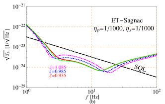
Figure 7: Plots showing the quantum NSD of polarizing Sagnac interferometers with different specifications for selected parameters. The configuration assumes the Sagnac interferometer parameters shown in Table 2. All plots are based on a default parameter set with detection angle $\theta=\pi/16$, homodyne detection angle $\zeta=0.935$ and $\eta_{s}=\eta_{p}=1/1000$. Part (a) shows the impacts of different extinction ratios $\eta_{s}$. $\eta_{p}$ is fixed, as it has little influence to the final results. Part (b) illustrates a narrow band quantum noise mitigation via a homodyne detection angle selection. Part (c) shows the noise spectrum for different detection ratio angles. The dashed green curves in all plots which are almost overlapped with those red curves (lossless Sagnac) illustrate the sensitivity of a lossy Sagnac interferometer when 75 ppm arm cavity round-trip loss being considered.

Parameter	Michelson	Sagnac
Arm length (L)	10 km	10 km
Input Power (after IMC)	3 W	15 W
Input Power at BS	138 W	690 W
Arm Cavity Power ($I_{c}$)	18 kW	180 kW
Temperature	10 K	20 K
Mirror Mass	211 kg	211 kg
Laser Wavelength	1550 nm	1550 nm
SR Detuning Phase	0.6	…
SR Transmittance	20%	…
Filter Cavities	2 $\times$ 10 km	…
Squeezed Level	10 dB	$\pm$10 dB
Scatter loss per surface	37.5 ppm	37.5 ppm

Table 2: A table summarizing the parameters of ET-LF interferometers. The Michelson values are taken from the design study Abernathy et al. (2011a). The Sagnac parameters proposed here refer to the high-power scenario with a circulating power of $I_{c}=180$ kW which gives the sensitivity shown in Fig. 4.

In Fig. 7, we show the resulting quantum NSD for different specifications of the parameters. We have assumed a default parameter base: (1) a small detection ratio angle $\theta=\pi/16$, (2) a homodyne detection angle $\zeta=0.935$, which gives an optimal sensitivity at a frequency around 10 Hz, (3) reasonable PBS extinction ratios $\eta_{s}=\eta_{p}=1/1000$, and (4) phase squeezing for the p-polarization, $r_{p}=0.5\ln 10$ and amplitude squeezing for the s-polarization, $r_{s}=-0.5\ln 10$. Figure 7 (a) shows the effects when various quality PBSs are implemented with $\theta=\pi/16$ and $\zeta=0.935$. In Fig. 7 (b) we keep $\eta_{s}=\eta_{p}=1/1000$ and $\theta=\pi/16$, and change the homodyne detection angle $\zeta$. Figure 7 (c) gives a possible detection ratio optimization when the leakage influences the quantum noise behavior. We have found that (i@) the low frequency quantum noise sensitivity greatly depends on the quality of the s-polarized reflection extinction ratio $\eta_{s}$, but is rarely impacted by the p-polarized transmission ratio $\eta_{p}$, given that $\eta_{s,p}$ are both smaller than 1%; (ii@) the homodyne detection angle can be optimized to slightly mitigate a narrow band quantum noise; (iii@) the losses have negligible impact on the sensitivity as one can imagine that the influence of the low-frequency losses are covered by the Michelson interferometer response. This is confirmed in each curve in Fig. 7, where the dashed green curve (illustrating the lossy Sagnac sensitivity) is almost identical to the solid lossless red curve; (iv@) the quantum noise behavior can be improved, as long as the Michelson output ensures the minimum DC requirement of the photodiode, which will be detailed in Sec. IV.

IV DC readout

The optical readout of a GW signal at the output of an interferometer requires a so-called local oscillator (LO), a reference light field which beats with the signal field on the photodiode. Current detectors use a concept called DC readout Hild et al. (2009) in which a part of the main circulating light field is directed into the dark port for this purpose. This concept has the advantage that the LO light is already prefiltered by the large baseline interferometer, on-axis and phase locked to the signal field.

In a Michelson interferometer the amount of carrier leakage into the dark port can be controlled with a small offset of the differential arm lengths. In an ideal Sagnac interferometer however, the dark fringe is independent of the mirror position. In the next section we investigate the possibility of generating a DC readout LO for the polarizing Sagnac interferometer. Additionally, we introduce a new method to select and control the homodyne detection angle for such an interferometer.

IV.1 Required light level and homodyne detection angle

The detected signal and the shot noise both scale as the square root of the LO power. In order to reach shot noise limited performance the light power in the LO must be large enough to (i) have the photodiode dark noise lower than the shot noise and (ii) dominate over waste light from higher order modes and stray light on the photodiode; it must also (iii) have the correct homodyne phase.

The exact light power required in the LO thus depends on the technical details of the interferometer implementation. The ET design has not yet reached such a level of detail and instead uses specifications for Advanced LIGO interferometers adl (2007); Abbott et al. (2010) as guidelines. In the following section, we focus with our investigation on the coupling of the fundamental mode into the detection port due to an intentional dark fringe offset and an arm imbalance Abbott et al. (2005).

It is reasonable to assume that stray light and photodiode dark noise will be similar in a Michelson and Sagnac interferometer. However, the coupling of light into the detection port has different origins in the two cases. In a Michelson interferometer it is caused by unequal losses in the two arms, but in a Sagnac interferometer it comes from a non-50:50 central BS. A 0.1% deviation from a perfect 50:50, which we consider reasonable to expect from a technical point of view, would lead coupling of $2\times 10^{-6}$ (relative to the circulating power at the central BS). This is larger than the Advanced LIGO estimate of $2\times 10^{-7}$, but as the Sagnac’s optimum homodyne angle ($\approx 53^{\circ}$) is further from $90^{\circ}$ (the signal) than the Michelson one ($\approx 100^{\circ}$), it can tolerate a higher ratio of light field (homodyne angle $0^{\circ}$ in both cases) to LO Abbott et al. (2005). In the following discussion, we therefore assume the same ratio of DC output power to central BS circulating power (which we call $\gamma$) as in Advanced LIGO, $1.75\times 10^{-5}$.

Below we consider two methods to achieve a similar LO light power in the Sagnac interferometer: (i) nonzero area Sagnac interferometers and (ii) PBS leakage.

IV.2 Sagnac area effect

A Sagnac interferometer with a nonzero area $\bf A$ responds to rotation $\Omega$ as

$$\Delta L=\frac{4{\bf A}\cdot{\rm\Omega}}{c},$$ (32)

where $c$ is the speed of light and $\Delta L$ is the same as shown in Eq. (27). The ratio $\gamma$ is

$$\gamma=\sin^{2}\left(\frac{2\pi\Delta L}{\lambda}\right).$$ (33)

When considering the Earth’s rotation, this corresponds to

$$\gamma=1.75\times 10^{-5}\left(\frac{A}{1350\,\rm m^{2}}\right)^{2}\left(\frac{1550\,\rm nm}{\lambda}\right)^{2}\left(\frac{\sin(\text{latitude})}{\sin(52^{\circ})}\right)^{2}.$$ (34)

The 1350 $\rm m^{2}$ area required for $\gamma=1.75\times 10^{-5}$ would have to be folded (requiring extra mirrors) to fit in the ET cavern; a 600 $\rm m^{2}$ loop (about the largest size that would fit as a four-mirror configuration) would have power fraction $\gamma=3.5\times 10^{-6}$. This method is also likely to give a suboptimal homodyne angle, as the strength of the LO is fixed by the loop size, and the homodyne angle is set by the ratio of this fixed LO strength to the (typically unknown prior to construction) light power due to an arm imbalance Abbott et al. (2005). Hence, we consider the PBS leakage method described in the next section to be more practical.

IV.3 PBS leakage light

As discussed in Sec. III.2, the leakage of an imperfect PBS creates a Michelson response signal. Here we consider the use of this field as the LO.

Figure 8: Diagrams illustrating a scheme of the outputs of two orthogonal polarized beams with an optical axis rotated PBS. The input beams contain both polarizations: p-polarized beam (arrow) and s-polarized beam (circle). The left diagram shows the optical layout at the detection port; the right diagram illustrates the output details by rotating the PBS’s polarization axes (p-s) by an angle $\theta$ (p^′-s^′).

If we measure two diagonal polarized beams after a PBS which has rotated polarization axes as shown in Fig. 8, we can choose the strength of the individual polarizations. With a rotation angle $\theta$, the output fields are

$$y =y_{p}\cos\theta+y_{s}\sin\theta,$$ (35)

$$y^{\prime} =y_{p}\sin\theta+y_{s}\cos\theta.$$ (36)

We know that the Michelson signal from the polarizing Sagnac interferometer is in the opposite polarization to the Sagnac signal. The parasitic Michelson interferometer has a circulating power $\eta_{s}$ times the Sagnac’s, and by setting it to bright fringe, we can send all of this to the output, which can be used as a LO [see Eq. (28)]. The output ratio from the Michelson leakage is

$$\gamma=\eta_{s}\sin^{2}\theta=1.75\times 10^{-5}\left(\frac{\eta_{s}}{0.001}\right)\left(\frac{\sin\theta}{0.13}\right)^{2}\,.$$ (37)

From Fig.7 (c) we have found that a small detection ratio is preferred, we choose $\theta=\pi/24$ such that $\gamma=1.75\times 10^{-5}$.

When the Michelson signal at the output is used as a LO for detection, the homodyne detection angle $\zeta$ is determined by the relative phase difference between the Sagnac signal (p-polarization) and the Michelson signal (s-polarization). In principle, the two responses are naturally in-phase at the detection port (see $q_{s}$ and $q_{p}$ in Fig. 7) and a wave plate (WP) can be used to shift the phase between them. The required homodyne detection angle then can be defined by a carefully chosen WP orientation and thickness. Compared to using an unknown amount of light due to an arm imbalance to define the homodyne detection angle, this method has obvious advantages.

IV.4 Potential control of a Sagnac with PBS leakage

In the current Michelson based GW detectors the positions of the mirrors have to be carefully controlled via error signals generated for different degrees of freedom (DoFs). In the Michelson we control PRCL (the length of the power recycling cavity); CARM (the common motion of the two arm cavities); DARM (the differential motion of the arm cavities); MICH (the Michelson differential length) and SRCL (the length of the signal recycling cavity). The DARM error signal is generated via DC readout whereas other error signals are obtained by adding RF sidebands to the input beam and demodulating these signals at various pickoff points within the detector. Common pickoff points include the reflection from the detector (REFL), between the BS and ITM of one of the arms (POX/Y) or at the antisymmetric output of the interferometer (AS).

The following is a preliminary investigation into error signals for controlling the proposed Sagnac interferometer. First, we consider which DoFs we require control of in our Sagnac detector. In the absence of a signal recycling mirror we do not require a control signal for SRCL. An initial consideration of the Sagnac output might suggest less tightly required control of some of the DoFs, notably DARM and MICH, as the light split at the BS travels through both arms, effectively keeping the interferometer consistently on the dark fringe. However, this will not be the case for a Sagnac acting as a GW detector. In this case we require tight control of the arms cavities to keep them on resonance and for our realistic approach we require control of the parasitic Michelson to prevent unreasonable fluctuations in our local oscillator. Therefore we expect to require good control signals for PRCL, CARM, DARM, and MICH.

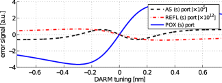
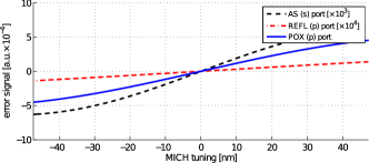
Figure 9: Plots showing preliminary error signals generated in Finesse for a realistic Sagnac detector, using ET-LF parameters and $\theta=\pi/24$, $\zeta=0.935$, $\eta_{s}=\eta_{p}=1/1000$ and with an increased arm cavity power of 180 kW. The different plots represent the signals for different degrees of freedom (DoFs), from top to bottom: PRCL, CARM, DARM, and MICH. For each DoF possible error signals are generated by applying control sidebands at 1.25 MHz and demodulating the signals at three different ports: AS (antisymmetric), REFL (reflected), and POX ($x$ arm pick off). The polarization of each signal (s or p) is indicated in the plot labels.

The output field of our realistic Sagnac interferometer ($q$) is in the p-polarization and contains mostly the Sagnac response, including any GW signal, with a small portion of light from the parasitic Michelson acting as a LO. The combination of the Sagnac and Michelson responses is achieved via a PBS and results in a second output signal, $q^{\prime}$ [see Fig. 5]. Unlike $q$, $q^{\prime}$ is s-polarized and dominated by the Michelson signal, containing just a small fraction of the Sagnac response. This signal is not used as the readout of the detector but could be used to control certain DoFs. Using the interferometer simulation tool Finesse, the polarized Sagnac was modeled using the realistic parameters $\theta=\pi/24$, $\zeta=0.935$ and $\eta_{s}=\eta_{p}=1/1000$ with an increased circulating arm power of 180 kW. RF sidebands of 1.25 MHz are added to the input beam. Error signals for the 4 degrees of freedom were produced by demodulating the two polarization fields at the AS, REFL, and POX ($x$ arm pickoff) ports.

In Fig. 9 we show some preliminary simulated error signals for the four DoFs; PRCL, CARM, DARM and MICH; required for our realistic Sagnac. The three ports investigated here demonstrate the potential for control of such a detector, with several possibilities for each DoF. This suggests a control scheme for a realistic Sagnac with PBS leakage could be realized in a similar manner to a conventional Michelson detector.

V Conclusion

It has previously been shown that a Sagnac interferometer without filter cavities can achieve a similarly low level of quantum noise at low frequencies as a Michelson with filter cavities Danilishin and Khalili (2012). We have built on this premise, presenting an alternative topology for the Einstein Telescope, replacing the Michelson interferometers of the low frequency detectors with Sagnac interferometers. Our scheme employs polarizing optics (a PBS and QWP) to direct the beam whilst being compatible with the current ET infrastructure and avoiding the technical problems caused by long ring-shape arm cavities.

We initially considered the performance of a Sagnac for ET-LF in the case of a perfect PBS and investigated the effects of losses on the performance, in terms of the quantum noise. Using the ET-LF parameters we found that the quantum-noise limited sensitivity of the Sagnac is better below 5 Hz but is reduced around the peak between 5 and 30 Hz. This reduction must be seen in the context of a greatly reduced complexity of the system that does not require filter cavities and signal recycling mirror. We showed that by increasing the circulating power by a factor of 10 we are able to achieve a comparable quantum noise with a Michelson with filter cavities, between 5 and 30 Hz, with even greater sensitivity below 5 Hz and discussed the feasibility of the higher power. We also find that including expected ET round-trip losses changes the quantum noise curve very little in the frequency band we are concerned with.

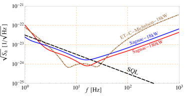
Figure 10: Plots comparing the quantum NSD of the proposed Sagnac topology (blue curve) against the ET-C Michelson topology based on same ET-LF Michelson parameters (See Table. 2). The Sagnac topology uses parameters $\theta=\pi/24$, $\zeta=0.935$ and $\eta_{s}=\eta_{p}=1/1000$ to ensure a LO for DC readout. Both Sagnac curves include the effects of optical losses, and the ET-C curve shown here does not consider optical losses in the filter cavities. The red curve shows a Sagnac with a higher power, 180 kW, circulating in the arm cavities, which would be a possible implementation to increase the peak sensitivity.

The main part of our investigation involved considering the effects and the possible operational advantages of a Sagnac with an imperfect PBS, specifically with a finite extinction ratio. By adapting our model to include the effects of a realistic PBS we demonstrated that the effect of a finite extinction ratio is described by the coupling of a Michelson signal onto the Sagnac input-output relation, where the signals of the Michelson and Sagnac are in the opposite polarizations. We found that the quantum noise of such an interferometer, at low frequencies, depends greatly on $\eta_{s}$, the extinction ratio of the reflection of the s-polarized beam and very little on $\eta_{p}$, the extinction ratio of the transmission of the p-polarized beam. This is due to the fact that s-polarized vacuum fluctuations are directly coupled in. Amplitude squeezed s-polarized squeezing light was revealed to be an effective approach to mitigate low-frequency quantum noise. As the quantum behavior of the Michelson at low frequencies is worse than the Sagnac, this combination of the two signals results in a degraded sensitivity. Again the impact of losses on the quantum noise performance was found to be negligible. We also found that the homodyne detection angle can be optimized to provide a broadband quantum noise reduction. Finally, we presented the quantum noise curve for a realistic candidate for a Sagnac interferometer for ET-LF (using an increased circulating power but otherwise retaining the original ET parameters). We consider a case with extinction ratios $\eta_{s}=\eta_{p}=1/1000$ and achieve a comparable quantum noise curve to a Michelson with filter cavities. The implementation of such an interferometer in the Einstein Telescope has significant implications for lowering costs and reducing the complexity which occurs with additional filter cavities, as well as the SR mirror. This topology also leaves room for further improvements and additional technologies, i.e., better suspensions and cryogenic mirrors.

The quantum noise behavior of the proposed Sagnac interferometer can be further improved by reducing the Michelson signal present in the detector output, by means of reducing the detection ratio angle. However, some of the Michelson signal is required to provide a LO for homodyne detection. Given the ET parameters we proposed, the absolute value of the LO power always ensures a lower photodiode dark noise compared to the shot noise. For our purpose, we used the Advanced LIGO ratio of DC output power to central BS circulating power, $1.75\times 10^{-5}$. We also considered using a nonzero Sagnac area interferometer to provide the required bias, but have found this to be impractical due to the large area required and suboptimal for homodyne angle selection. The leaked DC light provided by the nonperfect PBS is convenient for providing the LO and choosing homodyne detection angle. The required LO level is achievable with realistic extinction ratios. With our parameters, a detection ratio angle of $\pi/24$ was proposed to improve the quantum noise behavior. The sensitivity of a Sagnac interferometer, which retains all the ET-LF Michelson parameters, can be achieved as shown in Fig. 10 (blue curve). A high-power Sagnac with, 180 kW inside the arm cavities, shows an improved sensitivity [Fig. 10 (red curve)]. This gives a comparable sensitivity to the ET- LF Michelson interferometer and should be considered here for its potential to further improve the sensitivity in the long term.

A specific homodyne detection can be precisely determined by using a wave plate to shift the phase between the Michelson signal and Sagnac signal. Additionally we have conducted a preliminary investigation into the possible error signals which could be used to control a realistic Sagnac interferometer with PBS leakage, including looking at potential error signals generated from the leaked light provided by the imperfect PBS. Potential error signals for the required degrees of freedom, PRCL, CARM, DARM, and MICH, were generated using Finesse. While the design of a full control scheme for the proposed Sagnac configuration is beyond the scope of this paper, our preliminary results are encouraging and suggest that a control scheme can be developed by utilizing the different interferometer responses of the light fields in the two polarization states.

VI Acknowledgements

This work has been supported by the Science and Technology Facilities Council (STFC). We would like to thank Haixing Miao, Yanbei Chen and Stefan Hild for useful discussions and Harald Lück, Stefan Danilishin, Farid Khalili, and Chiara Mingarelli for comments and suggestions. This document has been assigned the LIGO Laboratory Document No. LIGO-P1300035.

Appendix A Optical System Block Diagram

A.1 Lossless free space propagation and single mirror reflection

Figure 11: Diagrams showing the schematics and the corresponding block diagrams of a light field (i) propagating in a free space and (ii) reflected by a single free hanging perfect mirror. $a$, $b$ and $a^{\prime}$, $b^{\prime}$ are the input and output variables, respectively. $\bf M_{pro}$ is the propagating input-output relation, $\bf M_{m}$ is the TF of a perfect mirror including the mechanical response and $\bf H_{m}$ is the GW signal TF, which couples in via the mirror’s motion. We denote $\bf{M}_{op}$ as the combination of the TFs of propagations and reflection.

A block diagram is convenient for the description of a system which consists of several principal parts. Each of them has a well-defined TF (or say input-output relation), in particular with an existing closed loop. Each block in the diagram represents each individual subsystem which is described by a specific TF. Different blocks are connected by arrows (including the signal flow direction), specifying the relationships between each blocks. Here we present the block diagrams of two simple optical systems: a laser beam (i) propagating in a free space and (ii) reflected by a signal free hanging perfect mirror as shown in Fig. 11. The GW single and radiation pressure force both act on the free mirror, inducing a displacement $x$. According to the propagation equations of an electromagnetic field, we thus have the output fields

$$\left[\begin{array}[]{c}b_{1}\\ b_{2}\end{array}\right]=\bf{M}_{pro}\cdot\left[\begin{array}[]{c}a_{1}\\ a_{2}\end{array}\right],$$ (42)

$$\left[\begin{array}[]{c}b^{\prime}_{1}\\ b^{\prime}_{2}\end{array}\right]=\bf{M}_{op}\cdot\left[\begin{array}[]{c}a^{\prime}_{1}\\ a^{\prime}_{2}\end{array}\right]+{\bf M}_{\rm pro}\cdot{\bf H_{m}}\cdot\rm h,$$ (47)

with

$${\bf M_{pro}}=e^{i\phi}\mathbf{R}[\varphi],\qquad{\bf M_{m}}=\left[\begin{array}[]{cc}1&0\\ -\kappa&1\end{array}\right],$$ (50)

$${\bf M}_{\rm op}=\bf{M}_{pro}\cdot\bf{M}_{m}\cdot{\bf M}_{pro},$$

$${\bf H_{m}}=\left[\begin{array}[]{c}0\\ \frac{\sqrt{2\kappa}}{h_{SQL}}\end{array}\right],\qquad\kappa=\frac{8I_{0}\omega_{0}}{mc^{2}\Omega^{2}},\qquad h_{SQL}=\sqrt{\frac{8\hbar}{m\Omega^{2}L^{2}}},$$ (53)

$$\mathbf{R}[\varphi]=\left[\begin{array}[]{cc}\cos\varphi&-\sin\varphi\\ \sin\varphi&\cos\varphi\end{array}\right],\qquad\phi=\frac{\Omega L}{c},\qquad\varphi=\frac{\omega_{0}L}{c}.$$ (56)

A.2 Lossless optical cavity

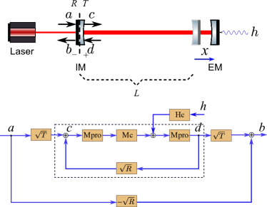
Figure 12: Diagram showing a schematic of an arbitrary lossless cavity and its block diagram. $a$, $b$, $c$ and $d$ represent light fields at different positions. $R$ and $T$ are the reflectivity and transmissivity of the cavity IM, which satisfy $R+T=1$ for the lossless case. The cavity EM is assumed to be perfect with a reflectivity equal to 1. A closed loop is formed due to the partial reflection of the IM. The GW signal and radiation pressure force act on the EM only.

With a similar process, we can describe an arbitrary lossless cavity ($R+T=1$) with a partially transmissive input mirror (IM) and a perfect end mirror (EM), as shown in Fig. 12. Because of both the transmission and reflection feature of the IM, a closed loop is formed (framed by the dashed box in the diagram). Based on the general TF evaluation of a system with a feedback loop, the TF of the dashed box can be written as

$${\bf M}_{\rm c}=\frac{1}{{\bf I}-\sqrt{R}\cdot\bf{M}_{\rm op}},$$ (57)

where ${\bf I}$ is the $2\times 2$ identity matrix and ${\bf M}_{op}$ is defined in Eq. (56).

A cavity being either resonant or detuned can be schematically described by the same diagram (see Fig. 12). The only difference comes from the propagation matrix $\rm M_{pro}$ due to different propagating lengths. Consequently, we obtain the general expression of the output field $b$ of a lossless cavity as

$$\left[\begin{array}[]{c}{b}_{1}(\Omega)\\ {b}_{2}(\Omega)\end{array}\right]= \left[-\sqrt{R}\cdot{\bf I}+T\cdot{\bf M}_{\rm c}\cdot\bf{M}_{\rm op}\right]\left[\begin{array}[]{c}{a}_{1}(\Omega)\\ {a}_{2}(\Omega)\end{array}\right]$$ (62)

$$+\left[\sqrt{T}\cdot{\bf M}_{\rm c}\cdot{\bf M}_{\rm pro}\cdot{\bf H}_{\rm c}\right]h(\Omega).$$ (63)

where ${\bf M}_{\rm pro}$, ${\bf M}_{\rm op}$, and ${\bf H}_{\rm c}$ are evaluated according to the variable definitions in Eq. (56). However, these parameters need to be modified as the laser power incident on the EM is different; ${\bf M}_{\rm c}$ is defined in Eq. (57). For a resonant cavity, the propagation matrix is

$${\bf M}_{\rm pro}^{\rm re}=e^{i\phi}.$$ (64)

The output field of a resonant lossless cavity can then be expressed by

$$\left[\begin{array}[]{c}{b}_{1}(\Omega)\\ {b}_{2}(\Omega)\end{array}\right]= e^{2i\phi_{cav}}\left[\begin{array}[]{cc}1&0\\ -\kappa_{cav}&1\end{array}\right]\left[\begin{array}[]{c}{a}_{1}(\Omega)\\ {a}_{2}(\Omega)\end{array}\right]$$ (71)

$$+e^{i\phi_{cav}}\frac{\sqrt{2\kappa_{cav}}}{h_{SQL}}\left[\begin{array}[]{c}0\\ 1\end{array}\right]h(\Omega),$$ (74)

with

$$\phi_{cav} =\arctan{(\frac{1+\sqrt{R_{i}}}{1-\sqrt{R_{i}}}}\tan{\Omega\tau)},$$ (75)

$$\kappa_{cav} =\frac{T_{i}\kappa}{1-2\sqrt{R_{i}}\cos(2\Omega\tau)+R_{i}}.\qquad$$ (76)

By inserting the distinctive propagation matrix of a detuned cavity with detuning phase $\theta$

$${\bf M}^{\rm de}_{\rm pro}=e^{i\phi}{\bf R}[\theta],$$ (77)

a similar output can be obtained. The outputs for both resonant and detuned cavities match with the results shown in Miao (2012).

A.3 Lossy optical cavity

Figure 13: Diagram showing a schematic of a lossy cavity and its corresponding block diagram. Both the IM and EM are partial transmissive mirrors. Cavity losses are grouped into the transmission of the EM, namely laser beams transmitted by the EM are considered as optical losses. Vacuum fluctuations $n$ simultaneously couple in due to these optical losses.The reflectivity and transmissivity of the mirrors still satisfy equation $T_{i,e}+R_{i,e}=1$. A mechanical displacement $x$ due to the circulating light radiation pressure force occurs only at the EM. The GW signal acts on the EM only.

We further consider the case of a cavity where optical losses have been included. It has been shown by previous work Kimble et al. (2001); Chen (2003); Purdue and Chen (2002); Purdue (2002) that additional vacuum fluctuations simultaneously enter into the optical system at different ports when there are optical losses. In our work, these optical loss induced vacuum fluctuations are grouped into one port, the cavity EM, and denoted as $n$. A similar schematic of a lossy cavity is shown in Fig. 13. We thus can write down the input-output relation of a lossy cavity as

$$\left[\begin{array}[]{c}{b}_{1}(\Omega)\\ {b}_{2}(\Omega)\end{array}\right]= \left[-\sqrt{R_{i}}\cdot{\bf I}+T_{i}\sqrt{R_{e}}\cdot{\bf M}_{\rm cav}^{*}\cdot\bf{M}_{\rm op}^{*}\right]\left[\begin{array}[]{c}{a}_{1}(\Omega)\\ {a}_{2}(\Omega)\end{array}\right]$$ (82)

$$+\left[\sqrt{T_{i}}\sqrt{R_{e}}\cdot{\bf M}_{\rm cav}^{*}\cdot{\bf M}_{\rm pro}\cdot{\bf H}_{\rm c}^{*}\right]h(\Omega),$$

$$+\left[\sqrt{T_{e}}\cdot{\bf M}_{\rm cav}^{*}\cdot{\bf M}_{\rm pro}\right]\left[\begin{array}[]{c}{n}_{1}(\Omega)\\ {n}_{2}(\Omega)\end{array}\right],$$ (85)

with

$${\bf M}_{\rm cav}^{*}=\frac{1}{{\bf I}-\sqrt{R_{i}R_{e}}\cdot\bf{M}_{\rm op}^{*}}.$$

$\bf{M}_{c}^{*}$, $\bf{M}_{\rm op}^{*}$, $\bf{H}_{c}^{*}$ have the same format as in the lossless expressions in Eqs. (56) and (57), but replacing $\kappa$ by

$$\kappa^{*}=\sqrt{R_{e}}\frac{8I^{*}\omega_{0}}{mc^{2}\Omega^{2}},$$ (86)

due to the EM loss, resulting in a lower laser power circulating inside the cavity. We assume the cavity loss is far smaller than 1, $T_{e}\ll 1$. This enables an approximation by keeping the leading order of $\sqrt{T_{e}}$ in the input-output relation. For a resonant lossy cavity, we thus get the same format input-output relation as Eq. (74):

$$\left[\begin{array}[]{c}{b}_{1}(\Omega)\\ {b}_{2}(\Omega)\end{array}\right]= e^{2i\phi_{cav}}\left[\begin{array}[]{cc}1&0\\ -\kappa_{cav}^{*}&1\end{array}\right]\left[\begin{array}[]{c}{a}_{1}(\Omega)\\ {a}_{2}(\Omega)\end{array}\right]$$ (93)

$$+e^{i\phi_{cav}}\frac{\sqrt{2\kappa_{cav}^{*}}}{h_{SQL}}\left[\begin{array}[]{c}0\\ 1\end{array}\right]h(\Omega)$$ (96)

$$\sqrt{T_{e}}e^{i\phi_{cav}}\sqrt{\frac{\kappa_{cav}^{*}}{\kappa^{*}}}\left[\begin{array}[]{cc}1&0\\ -\sqrt{\frac{\kappa_{cav}^{*}}{T_{i}}}e^{i\phi_{cav}-i\Omega\tau}&1\end{array}\right]\left[\begin{array}[]{c}{n}_{1}(\Omega)\\ {n}_{2}(\Omega)\end{array}\right].$$ (101)

We turn this input-output relation into

$$\left[\begin{array}[]{c}{b}_{1}(\Omega)\\ {b}_{2}(\Omega)\end{array}\right]={\bf M}_{\rm cav}\left[\begin{array}[]{c}{a}_{1}(\Omega)\\ {a}_{2}(\Omega)\end{array}\right]+{\bf H}_{\rm cav}h(\Omega)+{\bf N}_{\rm cav}\left[\begin{array}[]{c}{n}_{1}(\Omega)\\ {n}_{2}(\Omega)\end{array}\right],$$ (102)

where ${\bf M}_{\rm cav}$, ${\bf H}_{\rm cav}$ and ${\bf N}_{\rm cav}$ correspond to the matrices in Eq. (101). This gives the general input-output relation expression of a lossy resonant cavity. We further simplify such a cavity into a new block diagram as shown in Fig. 14, which can be recalled by any optical system containing a resonant cavity (i.e., interferometer arm cavities).

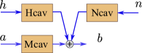
Figure 14: A block diagram of a general lossy resonant optical cavity. The TFs are defined in Eqs. (101) and (102).

Appendix B Imperfect Polarizing beamsplitter

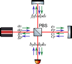
Figure 15: Figure showing the relations of polarized light fields at the four ports of a PBS. Subscripts $s$ and $p$ represent the polarization of each field. The arrows denote the p-polarized (blue) and s-polarized (green) beams. The PBS has an extinction ratio of $\eta_{p}$ for the transmitted p-polarized beam and $\eta_{s}$ for the reflected s-polarized beam.

Here we specify the relations of the transmission and reflection fields at a polarizing beam splitter (PBS). The PBS as shown in Fig. 15 has an extinction ratio of $\eta_{p}$ for the transmitted p-polarized beam and $\eta_{s}$ for the reflected s-polarized beam. Therefore, the relations between the input and output fields are

$$e_{s}= \sqrt{\eta_{s}}\cdot a_{s}+\sqrt{1-\eta_{s}}\cdot d_{s},$$

$$e_{p}= \sqrt{\eta_{p}}\cdot d_{p}+\sqrt{1-\eta_{p}}\cdot a_{p},$$

$$f_{s}= \sqrt{\eta_{s}}\cdot b_{s}+\sqrt{1-\eta_{s}}\cdot c_{s},$$

$$f_{p}= \sqrt{\eta_{p}}\cdot c_{p}+\sqrt{1-\eta_{p}}\cdot b_{p},$$

$$g_{s}= \sqrt{\eta_{s}}\cdot c_{s}+\sqrt{1-\eta_{s}}\cdot b_{s},$$

$$g_{p}= \sqrt{\eta_{p}}\cdot b_{p}+\sqrt{1-\eta_{p}}\cdot c_{p},$$

$$h_{s}= \sqrt{\eta_{s}}\cdot d_{s}+\sqrt{1-\eta_{s}}\cdot a_{s},$$

$$h_{p}= \sqrt{\eta_{p}}\cdot a_{p}+\sqrt{1-\eta_{p}}\cdot d_{p}.$$

The reflected p-polarized beams and transmitted s-polarized beams are also called leakages.

Appendix C Noise spectral density

With a well-defined input-output relation of an optical system, we can write the quadrature equation in a general form as

$$\left[\begin{array}[]{c}{b}_{1}(\Omega)\\ {b}_{2}(\Omega)\end{array}\right]= \left[\begin{array}[]{cc}M_{11}&M_{12}\\ M_{21}&M_{22}\end{array}\right]\left[\begin{array}[]{c}{a}_{1}(\Omega)\\ {a}_{2}(\Omega)\end{array}\right]+\left[\begin{array}[]{c}D_{1}\\ D_{2}\end{array}\right]h(\Omega)$$ (111)

$$+\left[\begin{array}[]{cc}N_{11}&N_{12}\\ N_{21}&N_{22}\end{array}\right]\left[\begin{array}[]{c}{n}_{1}(\Omega)\\ {n}_{2}(\Omega)\end{array}\right],$$ (116)

where each transfer matrix element is determined by a specific optical layout, with the first item being the vacuum fluctuations of the light field (i.e., laser beam), the second item being the GW signal and the third one the vacuum fluctuation induced by optical losses. Homodyne detection offers a possible selection of the readout as

$${b}_{\zeta}(\Omega)={b}_{1}(\Omega)\cos\zeta+{b}_{2}(\Omega)\sin\zeta,$$ (117)

with the homodyne detection angle $\zeta$. Correspondingly, the GW strain $h$-normalized quantum NSD of this measurement is defined as

$$S_{h}(\Omega)=\frac{(\cos\zeta,\sin\zeta){\bf M\cdot(S_{a}+S_{n})\cdot M}^{\rm{\dagger}}(\cos\zeta,\sin\zeta)^{T}}{|D_{1}\cos\xi+D_{2}\sin\xi|^{2}},$$ (118)

where $n$ is the optical loss induced vacuum fluctuations. The NSD matrix ${\bf S_{n}}$ thus is always an identity matrix. ${\bf S_{a}}$ is NSD matrix induced by the laser fluctuations and the elements are the corresponding NSD defined in Kimble et al. (2001) as

$${\bf S_{a}}(\Omega)=\left[\begin{array}[]{cc}S_{a_{1}a_{1}}(\Omega)&S_{a_{1}a_{2}}(\Omega)\\ S_{a_{2}a_{1}}(\Omega)&S_{a_{2}a_{2}}(\Omega)\end{array}\right],$$ (119)

with $\pi S_{a_{i}a_{j}}(\Omega)\delta(\Omega-\Omega^{\prime})=\langle\rm{in}|{a}_{i}(\Omega){a}^{{\dagger}}_{j}(\Omega^{\prime})|\rm{in}\rangle_{sym}$, i.e., if $|\rm{in}\rangle$ is a vacuum input $|0\rangle$, then $S_{a_{1}a_{1}}(\Omega)=S_{a_{2}a_{2}}(\Omega)=1$ and $S_{a_{1}a_{2}}(\Omega)=S_{a_{2}a_{1}}(\Omega)=0$ lead to an identity matrix ${\bf S}_{a}={\bf S}_{\rm vac}={\bf I}$.

Appendix D Complete equations

Here we present the complete equations of the two polarized output fields from a Sagnac interferometer with an imperfect PBS [see Eqs. (21) and (22)].

$$\left[\begin{array}[]{c}{q}_{p1}(\Omega)\\ {q}_{p2}(\Omega)\end{array}\right]= \left[-\sqrt{\eta_{p}}{\bf I}+(1-\eta_{p})\sqrt{1-\eta_{s}}{\bf M}_{\rm CLG}{\bf M}_{\rm sag}\right]\left[\begin{array}[]{c}{g}_{p1}(\Omega)\\ {g}_{p2}(\Omega)\end{array}\right]$$ (124)

$$+\sqrt{1-\eta_{p}}\sqrt{\eta_{s}}{\bf M}_{\rm CLG}{\bf M}_{\rm arm}\left[\begin{array}[]{c}{g}_{s1}(\Omega)\\ {g}_{s2}(\Omega)\end{array}\right]$$ (127)

$$+\sqrt{1-\eta_{p}}\sqrt{1-\eta_{s}}{\bf M}_{\rm CLG}{\bf H}_{\rm sag}h(\Omega)$$

$$+\sqrt{1-\eta_{p}}\sqrt{1-\eta_{s}}{\bf M}_{\rm CLG}{\bf N}_{\rm sag}\left[\begin{array}[]{c}{n}_{1}(\Omega)\\ {n}_{2}(\Omega)\end{array}\right]\,,$$ (130)

$$\left[\begin{array}[]{c}{q}_{s1}(\Omega)\\ {q}_{s2}(\Omega)\end{array}\right]= -\left[-\sqrt{1-\eta_{s}}{\bf I}+\eta_{s}\sqrt{\eta_{p}}{\bf M}_{\rm CLG}{\bf M}_{\rm sag}\right]\left[\begin{array}[]{c}{g}_{s1}(\Omega)\\ {g}_{s2}(\Omega)\end{array}\right]$$ (135)

$$+\sqrt{\eta_{s}}\sqrt{1-\eta_{p}}{\bf M}_{\rm CLG}{\bf M}_{\rm arm}\left[\begin{array}[]{c}{g}_{p1}(\Omega)\\ {g}_{p2}(\Omega)\end{array}\right]$$ (138)

$$+\sqrt{\eta_{s}}{\bf M}_{\rm CLG}{\bf H}_{\rm arm}h(\Omega)$$

$$+\sqrt{\eta_{s}}{\bf M}_{\rm CLG}{\bf N}_{\rm arm}\left[\begin{array}[]{c}{n}_{1}(\Omega)\\ {n}_{2}(\Omega)\end{array}\right].$$ (141)

References

- Harry and the LIGO Scientific Collaboration (2010) G. M. Harry and the LIGO Scientific Collaboration, Classical and Quantum Gravity 27, 084006 (2010), URL http://stacks.iop.org/0264-9381/27/i=8/a=084006.
- Accadia et al. (2011) T. Accadia, F. Acernese, F. Antonucci, P. Astone, G. Ballardin, F. Barone, M. Barsuglia, A. Basti, T. S. Bauer, M. Bebronne, et al., Classical and Quantum Gravity 28, 114002 (2011), URL http://stacks.iop.org/0264-9381/28/i=11/a=114002.
- Sathyaprakash et al. (2012) B. Sathyaprakash, M. Abernathy, F. Acernese, P. Ajith, B. Allen, P. Amaro-Seoane, N. Andersson, S. Aoudia, K. Arun, P. Astone, et al., Classical and Quantum Gravity 29, 124013 (2012), URL http://stacks.iop.org/0264-9381/29/i=12/a=124013.
- Shoemaker (2001) D. Shoemaker, Future limits to sensitivity, presentation given at the Aspen Workshop (2001), URL https://dcc.ligo.org/DocDB/0033/G010026/000/G010026-00.pdf.
- Hild et al. (2010) S. Hild, S. Chelkowski, A. Freise, J. Franc, N. Morgado, R. Flaminio, and R. DeSalvo, Classical and Quantum Gravity 27, 015003 (8pp) (2010), URL http://stacks.iop.org/0264-9381/27/015003.
- Sagnac (1913) G. Sagnac, Comptes Rendus 157, 708 (1913), URL http://en.wikisource.org/wiki/The_Demonstration_of_the_Luminiferous_Aether.
- Sun et al. (1996) K.-X. Sun, M. M. Fejer, E. Gustafson, and R. L. Byer, Phys. Rev. Lett. 76, 3053 (1996), URL http://link.aps.org/doi/10.1103/PhysRevLett.76.3053.
- Petrovichev et al. (1998) B. Petrovichev, M. Gray, and D. McClelland, General Relativity and Gravitation 30, 1055 (1998), ISSN 0001-7701, 10.1023/A:1026600721872, URL http://dx.doi.org/10.1023/A:1026600721872.
- Beyersdorf et al. (1999a) P. T. Beyersdorf, M. M. Fejer, and R. L. Byer, Opt. Lett. 24, 1112 (1999a), URL http://ol.osa.org/abstract.cfm?URI=ol-24-16-1112.
- Beyersdorf et al. (1999b) P. T. Beyersdorf, M. M. Fejer, and R. L. Byer, J. Opt. Soc. Am. B 16, 1354 (1999b), URL http://josab.osa.org/abstract.cfm?URI=josab-16-9-1354.
- Mizuno et al. (1997) J. Mizuno, A. Rüdiger, R. Schilling, W. Winkler, and K. Danzmann, Optics Communications 138, 383 (1997), ISSN 0030-4018, URL http://www.sciencedirect.com/science/article/B6TVF-497C654-120/2/9ed770e7f770ad7e189a36c723bd7823.
- Abernathy et al. (2011a) M. Abernathy, F. Acernese, P. Ajith, B. Allen, P. Amaro-Seoane, N. Andersson, S. Aoudia, P. Astone, B. Krishnan, L. Barack, et al., p. 451(18) (2011a), URL http://www.et-gw.eu/etdsdocument.
- Chen (2003) Y. Chen, Phys. Rev. D 67, 122004 (2003), URL http://link.aps.org/doi/10.1103/PhysRevD.67.122004.
- Danilishin (2004) S. L. Danilishin, Phys. Rev. D 69, 102003 (2004), URL http://link.aps.org/doi/10.1103/PhysRevD.69.102003.
- Chen et al. (2011) Y. Chen, S. Danilishin, F. Khalili, and H. Müller-Ebhardt, General Relativity and Gravitation 43, 671 (2011), eprint arXiv:0910.0319, URL http://link.springer.com/article/10.1007%2Fs10714-010-1060-y.
- Danilishin and Khalili (2012) S. L. Danilishin and F. Y. Khalili, Living Reviews in Relativity 15 (2012), URL http://www.livingreviews.org/lrr-2012-5.
- Wade et al. (2012) A. R. Wade, K. McKenzie, Y. Chen, D. A. Shaddock, J. H. Chow, and D. E. McClelland, Phys. Rev. D 86, 062001 (2012), URL http://link.aps.org/doi/10.1103/PhysRevD.86.062001.
- Eberle et al. (2010) T. Eberle, S. Steinlechner, J. Bauchrowitz, V. Händchen, H. Vahlbruch, M. Mehmet, H. Müller-Ebhardt, and R. Schnabel, Phys. Rev. Lett. 104, 251102 (2010), URL http://link.aps.org/doi/10.1103/PhysRevLett.104.251102.
- Müller-Ebhard et al. (2009) H. Müller-Ebhard, H. Rehbein, S. Hild, A. Freise, Y. Chen, R. Schnabe, K. Danzmann, and H. Lück, ET note ET-010-09 (2009), URL https://workarea.et-gw.eu/et/WG5-Management/et-codified-documents/et-document-codifier.
- adl (2007) Advanced ligo reference design, LIGO Technical report M060056 (2007), URL http://www.ligo.caltech.edu/docs/M/M060056-08/M060056-08.pdf.
- Ward et al. (2008) R. L. Ward, R. Adhikari, B. Abbott, R. Abbott, D. Barron, R. Bork, T. Fricke, V. Frolov, J. Heefner, A. Ivanov, et al., Classical and Quantum Gravity 25, 114030 (2008), ISSN 0264-9381, URL http://stacks.iop.org/0264-9381/25/i=11/a=114030.
- Hild et al. (2009) S. Hild, H. Grote, J. Degallaix, S. Chelkowski, K. Danzmann, A. Freise, M. Hewitson, J. Hough, H. Luck, M. Prijatelj, et al., Classical and Quantum Gravity 26, 055012 (10pp) (2009), URL http://stacks.iop.org/0264-9381/26/055012.
- Fricke et al. (2012) T. T. Fricke, N. D. Smith-Lefebvre, R. Abbott, R. Adhikari, K. L. Dooley, M. Evans, P. Fritschel, V. V. Frolov, K. Kawabe, J. S. Kissel, et al., Classical and Quantum Gravity 29, 065005 (2012), ISSN 0264-9381, URL http://stacks.iop.org/0264-9381/29/i=6/a=065005.
- Freise et al. (2004) A. Freise, G. Heinzel, H. Lück, R. Schilling, B. Willke, and K. Danzmann, Classical and Quantum Gravity 21, S1067 (2004), URL http://stacks.iop.org/0264-9381/21/S1067.
- (25) A. Freise, Finesse webpage, http://www.gwoptics.org/finesse, URL http://www.gwoptics.org/finesse.
- Kimble et al. (2001) H. J. Kimble, Y. Levin, A. B. Matsko, K. S. Thorne, and S. P. Vyatchanin, Phys. Rev. D 65, 022002 (2001), URL http://link.aps.org/doi/10.1103/PhysRevD.65.022002.
- Abernathy et al. (2011b) M. Abernathy, F. Acernese, P. Ajith, B. Allen, P. Amaro-Seoane, N. Andersson, S. Aoudia, P. Astone, B. Krishnan, L. Barack, et al., pp. 451(150–155) (2011b), URL http://www.et-gw.eu/etdsdocument.
- Abbott et al. (2010) R. Abbott, R. Adhikari, S. Ballmer, L. Barsotti, M. Evans, P. Fritschel, V. Frolov, G. Mueller, B. Slagmolen, and S. Waldman, Advanced LIGO note (2010), URL https://dcc.ligo.org/public/0012/T1000298/002/lscfdd.pdf.
- Abbott et al. (2005) B. Abbott, R. Adhikari, D. Busby, J. Heefner, K. Kawabe, O. Miyakawa, V. Sannibale, M. Smith, M. Varvella, S. Vass, et al., Advanced LIGO note (2005), URL www.ligo.caltech.edu/~cit40m/Docs/40mDCdetect.pdf.
- Miao (2012) H. Miao, Exploring Macroscopic Quantum Mechanics in Optomechanical Devices, Springer Thesis (Springer Berlin Heidelberg, 2012), ISBN 9783642256400, URL http://books.google.de/books?id=Myo8jXpvx2sC.
- Purdue and Chen (2002) P. Purdue and Y. Chen, Phys. Rev. D 66, 122004 (2002), URL http://link.aps.org/doi/10.1103/PhysRevD.66.122004.
- Purdue (2002) P. Purdue, Phys. Rev. D 66, 022001 (2002), URL http://link.aps.org/doi/10.1103/PhysRevD.66.022001.