‘Truncate, replicate, sample’: a method for creating integer weights for spatial microsimulation

Abstract

Iterative proportional fitting (IPF) is a widely used method for spatial microsimulation. The technique results in non-integer weights for individual rows of data. This is problematic for certain applications and has led many researchers to favour combinatorial optimisation approaches such as simulated annealing. An alternative to this is ‘integerisation’ of IPF weights: the translation of the continuous weight variable into a discrete number of unique or ‘cloned’ individuals. We describe four existing methods of integerisation and present a new one. Our method — ‘truncate, replicate, sample’ (TRS) — recognises that IPF weights consist of both ‘replication weights’ and ‘conventional weights’, the effects of which need to be separated. The procedure consists of three steps: 1) separate replication and conventional weights by truncation; 2) replication of individuals with positive integer weights; and 3) probabilistic sampling. The results, which are reproducible using supplementary code and data published alongside this paper, show that TRS is fast, and more accurate than alternative approaches to integerisation.

1 Introduction

Spatial microsimulation has been widely and increasingly used as a term to describe a a set of techniques used to estimate the characteristics of individuals within geographic zones about which only aggregate statistics are available (Tanton and Edwards, 2012; Ballas et al., 2013). The model inputs operate on a different level from those of the outputs. To ensure that the individual-level output matches the aggregate inputs, spatial microsimulation mostly relies on one of two methods. Combinatorial optimisation algorithms are used to select a unique combination of individuals from a survey dataset. This approach was first demonstrated and applied by Williamson et al. (1998) and there have been several applications and refinements since then. Alternatively, deterministic reweighting iteratively alters an array of weights, $N$, for which columns and rows correspond to zones and individuals, to optimise the fit between observed and simulated results at the aggregate level. This approach has been implemented using iterative proportional fitting (IPF) to combine national survey data with small area statistics tables (e.g. Beckman et al., 1996; Ballas et al., 2005a). A recent review, published in this journal, highlights the advances made in methods for simulating spatial microdata (Hermes and Poulsen, 2012) since these works were published. Harland et al. (2012) also discuss the state of spatial microsimulation research and present a comparative critique of the performance of deterministic reweighting and combinatorial optimisation methods. Both approaches require micro-level and spatially aggregated input data and a predefined exit point: the fit between simulated and observed results improves, at a diminishing rate, with each iteration.

The benefits of IPF include speed of computation, simplicity and the guarantee of convergence (Deming, 1940; Mosteller, 1968; Fienberg, 1970; Wong, 1992; Pritchard and Miller, 2012). A major potential disadvantage, however, is that non-integer weights are produced: fractions of individuals are present in a given area whereas after combinatorial optimisation, they are either present or absent. Although this is not a problem for many static spatial microsimulation applications (e.g. estimating income at the small area level, at one point in time; for example see Anderson 2013), several applications require integer rather than fractional weights. For example, integer weights are required if a population is to be simulated dynamically into the future (e.g. Ballas et al., 2005a; Clarke, 1986; Holm et al., 1996; Hooimeijer, 1996) or linked to agent-based models (e.g. Birkin and Clarke, 2011; Gilbert, 2008; Gilbert and Troitzsch, 2005; Wu et al., 2008; Pritchard and Miller, 2012).

Integerisation solves this problem by converting the weights — a 2D array of positive real numbers ($N\in\mathbb{R}_{\geq 0}$) — into an array of integer values ($N^{\prime}\in\mathbb{N}$) that represent whether the associated individuals are present (and how many times they are replicated) or absent. The integerisation function must perform $f(N)=N^{\prime}$ whilst minimizing the difference between constraint variables and the aggregated results of the simulated individuals. Integerisation has been performed on the results of the SimBritain model, based on simple rounding of the weights and two deterministic algorithms that are evaluated subsequently in this paper (see Ballas et al., 2005a). It was found that integerisation “resulted in an increase of the difference between the ‘simulated’ and actual cells of the target variables” (Ballas et al., 2005a, p. 26), but there was no further analysis of the amount of error introduced, or which integerisation algorithm performed best.

To the best of our knowledge, no published research has quantitatively compared the effectiveness of different integerisation strategies. We present a new method — truncate, replicate sample (TRS) — that combines probabilistic and deterministic sampling to generate representative integer results. The performance of TRS is evaluated alongside four alternative methods.

An important feature of this paper is the provision of code and data that allow the results to be tested and replicated using the statistical software R (R Core Team, 2012). Reproducible research can be defined as that which allows others to conduct at least part of the analysis (Table 1). Best practice is well illustrated by Williamson (2007), an instruction manual on combinatorial optimisation algorithms described in previous work. Reproducibility is straightforward to achieve (Gentleman and Temple Lang, 2007), has a number of important benefits (Ince et al., 2012), yet is often lacking in the field.

Table 1: Criteria for reproducible research, adapted from Peng et al. (2006)

Research component	Criteria
Data	Make dataset available, either in original form or in anonymous, scrambled form if confidential
Methods	Make code available for data analysis. Use non-prohibitive software if possible
Documentation	Provide comments in code and describe how to replicate results
Distribution	Provide a mechanism for others to access data, software, and documentation

The next section reviews the wider context of spatial microsimulation research and explains the importance of integerisation. The need for new methods is established in Section 3, which describes increasingly sophisticated methods for integerising the results of IPF. Comparison of these five integerisation methods show TRS to be more accurate than the alternatives, across a range of measures (Section 4). The implications of these findings are discussed in Section 5.

2 Spatial microsimulation: the state of the art

2.1 What is spatial microsimulation, and why use it?

Spatial microsimulation is a modelling method that involves sampling rows of survey data (one row per individual, household, or company) to generate lists of individuals (or weights) for geographic zones that expand the survey to the population of each geographic zone considered. The problem that it overcomes is that most publicly available census datasets are aggregated, whereas individual-level data are sometimes needed. The ecological fallacy (Openshaw, 1983), for example, can be tackled using individual-level data.

Microsimulation cannot replace the ‘gold standard’ of real, small area microdata (Rees et al., 2002, p. 4), yet the method’s practical usefulness (see Tomintz et al., 2008) and testability (Edwards and Clarke, 2009) are beyond doubt. With this caveat in mind, the challenge can be reduced to that of optimising the fit between the aggregated results of simulated spatial microdata and aggregated census variables such as age and sex (Williamson et al., 1998). These variables are often referred to as ‘constraint variables’ or ‘small area constraints’ (Hermes and Poulsen, 2012). The term ‘linking variables’ can also be used, as they link aggregate and survey data.

The wide range of methods available for spatial microsimulation can be divided into static, dynamic, deterministic and probabilistic approaches (Table 2.1). Static approaches generate small area microdata for one point in time. These can be classified as either probabilistic methods which use a random number generator, and deterministic reweighting methods, which do not. The latter produce fractional weights. Dynamic approaches project small area microdata into the future. They typically involve modelling of life events such as births, deaths and migration on the basis of random sampling from known probabilities on such events (Ballas et al., 2005a; Vidyattama and Tanton, 2010); more advanced agent-based techniques, such as spatial interaction models and household-level phenomena, can be added to this basic framework (Wu et al., 2008, 2010). There are also ‘implicitly dynamic’ models, which employ a static approach to reweight an existing microdata set to match projected change in aggregate-level variables (e.g. Ballas et al., 2005b).

Table 2: Typology of spatial microsimulation methods

Type	Reweighting technique	Pros	Cons	Example
Determ- inistic Re- weighting	Iterative proportional fitting (IPF)	Simple, fast, accurate, avoids local optima and random numbers	Non-integer weights	(Tomintz et al., 2008)⁠⁠
	Integerised IPF	Builds on IPF, provides integer weights	Integerisation reduces model fit	(Ballas et al., 2005a)⁠
	GREGWT, generalised reweighting	Fast, accurate, avoids local optima and random numbers	Non-integer weights	(Miranti et al., 2010)⁠
Probab- ilistic Combin- atorial optim- isation	Hill climbing approach	The simplest solution to a combinatorial optimisation, integer results	Can get stuck in local optima, slow	(Williamson et al., 1998)⁠
	Simulated annealing	Avoids local minima, widely used, multi-level constraints	Computationally intensive	(Kavroudakis et al., 2012)⁠
Dynamic	Monte Carlo randomisation to simulate ageing	Realistic treatement of stochastic life events such as death	Depends on accurate estimates of life event probabilities	(Vidyattama and Tanton, 2010)⁠
	Implicitly dynamic	Simplicity, low computational demands	Crude, must project constraint variables	(Ballas et al., 2005c)⁠

2.2 IPF-based Monte Carlo approaches for the generation of synthetic microdata

Individual-level, anonymous samples from major surveys, such as the Sample of Anonymised Records (SARs) from the UK Census have only been available since around the turn of the century (Li, 2004). Beforehand, researchers had to rely on synthetic microdata. These can be created using probabilistic methods (Birkin and Clarke, 1988). The iterative proportional fitting (IPF) technique was first described in 1940 (Deming, 1940), and has become well established for spatial microsimulation (Axhausen and Müller, 2010; Birkin and Clarke, 1989).

The first application of IPF in spatial microsimulation was presented by Birkin and Clarke (1988 and 1989) to generate synthetic individuals, and allocate them to small areas based on aggregated data. They produced spatial microdata (a list of individuals and households for each electoral ward in Leeds Metropolitan District). Their approach was to select rows of synthetic data using Monte Carlo sampling. Birkin and Clarke suggested that the microdata generation technique known as ‘population synthesis’ could be of great practical use (Birkin and Clarke, 2012).

2.3 Combinatorial optimisation approaches

Since the work of Birkin and Clarke (1988 and 1989) there have been considerable advances in data availability and computer hardware and software. In particular, with the emergence of anonymous survey data, the focus of spatial microsimulation shifted towards methods for reweighting and sampling from existing microdata, as opposed to the creation of entirely synthetic data (Lee, 2009).

This has enabled experimentation with new techniques for small area microdata generation. A significant contribution to the literature was made by Williamson et al. (1998). The authors presented microsimulation as a problem of combinatorial optimisation: finding the combination of SARs which best fits the constraint variables. Various approaches to combinatorial optimisation were compared, including ‘hill climbing’, simulated annealing approaches and genetic algorithms (Williamson et al., 1998). These approaches involve the selection and replication of a discrete number of individuals from a nationally representative list such as the SARs. Thus, subsets of individuals are taken from the global microdataset (geocoded at coarse geographies) and allocated to small areas. There have been several refinements and applications of the original ideas suggested by Williamson et al. (1998), including research reported by Voas and Williamson (2000), Williamson et al. (2002), and Ballas et al. (2006).

2.4 Deterministic reweighting

The methods described in the previous section involve the use of random sampling procedures or ‘probabilistic reweighting’ (Hermes and Poulsen, 2012). In contrast, Ballas et al. (2005c) presented an alternative deterministic approach based on IPF. It is the results of this method, that does not use random number generators and thus produces the same output with each run, that the integerisation methods presented here take as their starting point. The underlying theory behind IPF has been described in a number of papers (Deming, 1940; Mosteller, 1968; Wong, 1992). Fienberg (1970) proves that IPF converges towards a single solution.

IPF can be used to produce maximum likelihood estimates of spatially disaggregated conditional probabilities for the individual attributes of interest. The method is also known as ‘matrix raking’, RAS or ‘entropy maximising’ (see Johnston and Pattie, 1993; Birkin and Clarke, 1988; Axhausen and Müller, 2010; Huang and Williamson, 2001; Kalantari et al., 2008; Jiroušek and Přeučil, 1995). The mathematical properties of IPF have have been described in several papers (see for instance Bishop et al., 1975; Fienberg, 1970; Birkin and Clarke, 1988). Illustrative examples of the procedure can be found in Saito (1992), Wong (1992) and Norman (1999). Wong (1992) investigated the reliability of IPF and evaluated the importance of different factors influencing its performance; Simpson and Tranmer (2005) evaluated methods for improving the performance of IPF-based microsimulation. Building on these methods, IPF has been employed by others to investigate a wide range of phenomena (e.g. Mitchell et al., 2000; Ballas et al., 2005a; Williamson et al., 2002; Tomintz et al., 2008).

Practical guidance on how to perform IPF for spatial microsimulation is also available. In an online working paper, Norman (1999) provides a user guide for a Microsoft Excel macro that performs IPF on large datasets. Simpson and Tranmer (2005) provided code snippets of their procedure in the statistical package SPSS. Ballas et al. (2005c) describe the process and how it can be applied to problems of small area estimation. In addition to these resources, a practical guide to running IPF in R has been created to accompany this paper.

2.5 Combinatorial optimisation, IPF and the need for integerisation

The aim of IPF, as with all spatial microsimulation methods, is to match individual-level data from one source to aggregated data from another. IPF does this repeatedly, using one constraint variable at a time: each brings the column and row totals of the simulated dataset closer to those of the area in question (see Ballas et al., 2005c and Fig. 5 below).

Unlike combinatorial optimisation algorithms, IPF results in non-integer weights. As mentioned above, this is problematic for certain applications. In their overview of methods for spatial microsimulation Williamson et al. (1998) favoured combinatorial optimisation approaches, precisely for this reason: “as non-integer weights lead, upon tabulation of results, to fractions of households or individuals” (p. 791). There are two options available for dealing with this problem with IPF:

• Use combinatorial optimisation microsimulation methods instead (Williamson et al., 1998). However, this can be computationally intensive (Pritchard and Miller, 2012).

• Integerise the weights: Translate the non-integer weights obtained through IPF into discrete counts of individuals selected from the original survey dataset (Ballas et al., 2005a).

We revisit the second option, which arguably provides the ‘best of both worlds’: the simplicity and computational speed of deterministic reweighting and the benefits of using whole cases.

In summary, IPF is an established method for combining microdata with spatially aggregated constraints to simulate target variables whose characteristics are not recorded at the local level. Intergerisation translates the real number weights obtained by IPF into samples from the original microdata, a list of ‘cloned’ individuals for each simulated area. Integerisation may also be useful conceptually, as it allows researchers to deal with entire individuals. The next section reviews existing strategies for integerisation.

3 Method

Despite the importance of integer weights for dynamic spatial microsimulation, and the continued use of IPF, there has been little work directed towards integerisation. It has been noted that “the integerization and the selection tasks may introduce a bias in the synthesized population” (Axhausen and Müller, 2010, 10), yet little work has been done to find out how much error is introduced.

To test each integerisation method, IPF was used to to generate an array of weights that fit individual-level survey data to geographically aggregated Census data (see Section 3.7). Five methods for integerising the results are described, three deterministic and two probabilistic. These are: ‘simple rounding’, its evolution into the ‘threshold approach’ and the ‘counter-weight’ method and the probabilistic methods ‘proportional probabilities’ and finally ‘truncate, replicate, sample’. TRS builds on the strengths of the other methods, hence the order in which they are presented.

The application of these methods to the same dataset (and their implementation in the same language, R) allows their respective performance characteristics to be quantified and compared. Before proceeding to describe the mechanisms by which these integerisation methods work, it is worth taking a step back, to consider the nature and meaning of IPF weights.

3.1 Interpreting IPF weights: replication and probability

It is important to clarify what we mean by ‘weights’ before proceeding to implement methods of integerisation: this understanding was central to the development of the integerisation method presented in this paper. The weights obtained through IPF are real numbers ranging from 0 to hundreds (the largest weight in the case study dataset is 311.8). This range makes integerisation problematic: if the probability of selection is proportional to the IPF weights (as is the case with the ‘proportional probabilities’ method), the majority of resulting selection probabilities can be very low. This is why the simple rounding method rounds weights up or down to the nearest integer weight to determine how many times each individual should be replicated (Ballas et al., 2005a): to ensure replication weights do not differ greatly from non-integer IPF weights. However, some of the information contained in the weight is lost during rounding: a weight remainder of 0.501 is treated the same as 0.999.

This raises the following question: Do the weights refer to the number of times a particular individual should be replicated, or is it related to the probability of being selected? The following sections consider different approaches to addressing this question, and the integerisation methods that result.

3.2 Simple rounding

The simplest approach to integerisation is to convert the non-integer weights into an integer by rounding. If the decimal remainder to the right of the decimal is 0.5 or above, the integer is rounded up; if not, the integer is rounded down.

Rounding alone is inadequate for accurate results, however. As illustrated in Fig. 2 below, the distribution of weights obtained by IPF is likely to be skewed, and the majority of weights may fall below the critical 0.5 value and be excluded. As reported by Ballas et al. (2005a, 25), this results in inaccurate total populations. To overcome this problem Ballas et al. (2005a) developed algorithms to ‘top up’ the simulated spatial microdata with representative individuals: the ‘threshold’ and ‘counter-weight’ approaches.

3.3 The threshold approach

Ballas et al. (2005a) tackled the need to ‘top up’ the simulated area populations such that $Pop_{sim}\geq Pop_{cens}$. To do this, an inclusion threshold ($IT$) is created, set to 1 and then iteratively reduced (by 0.001 each time), adding extra individuals with incrementally lower weights. Below the exit value of $IT$ for each zone, no individuals can be included (hence the clear cut-off point around 0.4 in Fig. 1). In its original form, based on rounded weights, this approach over-replicates individuals with high decimal weights. To overcome this problem, we took the truncated weights as the starting population, rather than the rounded weights. This modified approach improved the accuracy of the integer results and is therefore what we refer to when the ‘threshold approach’ is mentioned henceforth.

The technique successfully tops-up integer populations yet has a tendency to generate too many individuals for each zone. This oversampling is due to duplicate weights — each unique weight was repeated on average 3 times in our model — and the presence of weights that are different, but separated by less than 0.001. (In our test, the mean number of unique weights falling into non-empty bins between 0.3 and 0.48 in each area — the range of values reached by $IT$ before $Pop_{sim}\geq Pop_{cens}$ — is almost two.)

3.4 The counter-weight approach

An alternative method for topping-up integer results arrived at by simple rounding was also described by Ballas et al. (2005a). The approach was labelled to emphasise its reliance on both counter and a weight variables. Each individual is first allocated a counter in ascending order of its IPF weight. The algorithm then tops-up the integer results of simple rounding by iterating over all individuals in the order of their count. With each iteration the new integer weight is set as the rounded weight plus the rounded sum of its decimal weight plus the decimal weight of the next individual, until the desired total population is reached.

There are two theoretical advantages of this approach: its more accurate final populations (it does not automatically duplicate individuals with equal weights as the threshold approach does) and the fact that individuals with decimal weights down to 0.25 may be selected. This latter advantage is minor, as $IT$ reached below 0.4 in many cases (Supplementary Information, Fig. 2) — not far off. A band of low weights (just above 0.25) selected by the counter-weight method can be seen in Fig. 1.

The total omission of weights below some threshold is problematic for all deterministic algorithms tested here: they imply that someone with a weight below this threshold, for example 0.199 in our tests, has the same sampling probability as someone with a weight of 0.001: zero! The complete omission of low weights fails to make use of all the information stored in IPF weights: in fact, the individual with an IPF weight of 0.199 is 199 times more representative of the area (in terms of the constraint variables and the make-up of the survey dataset) than the individual with an IPF weight of 0.001. Probabilistic approaches to integerisation ensure that all such differences between decimal weights are accounted for.

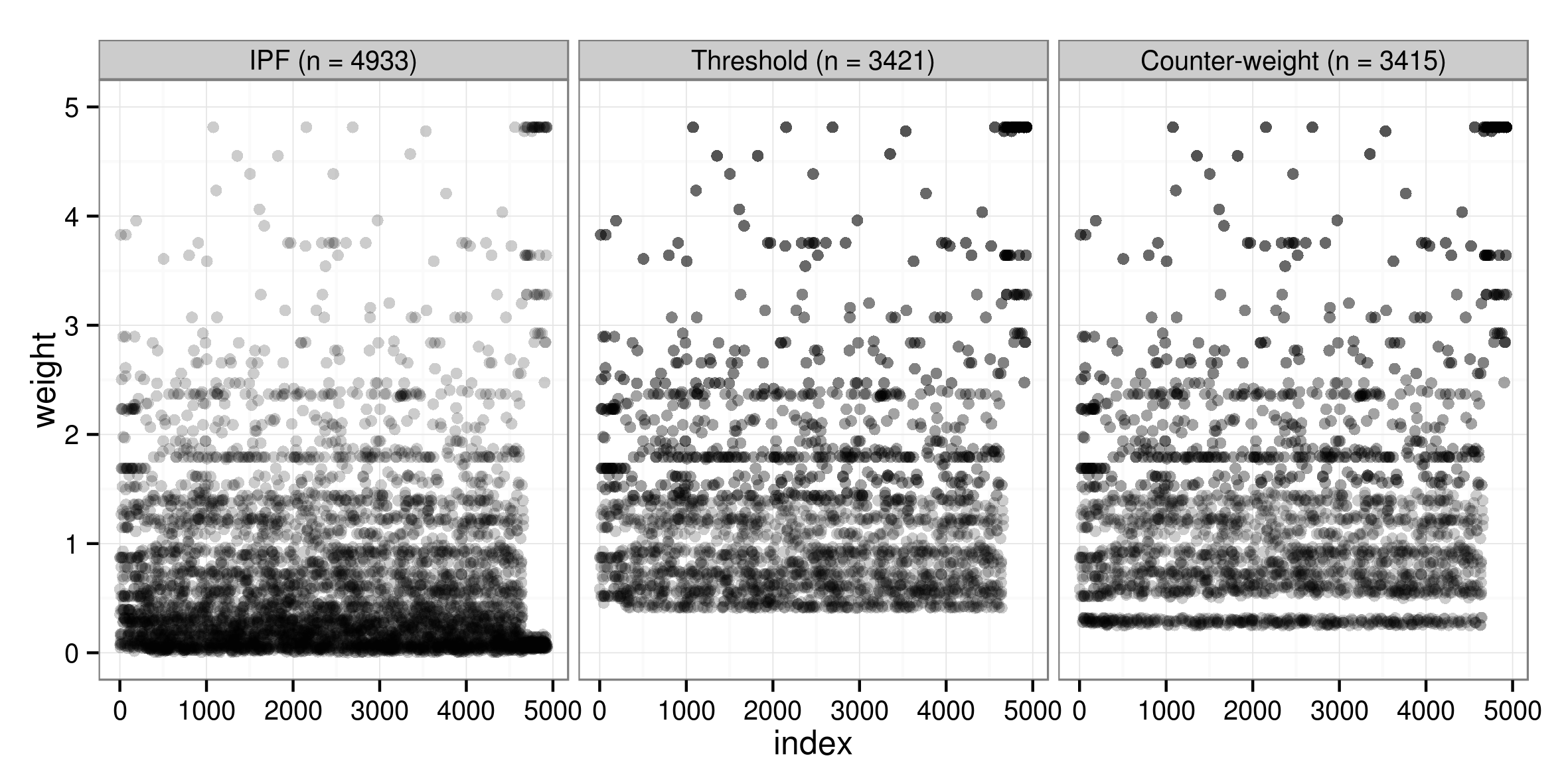
Figure 1: Overplotted scatter graph showing the distribution of weights and replications after IPF in the original survey (left), those selected by inclusion thresholds for a single area (middle), and those selected by the counter-weight method (right) for zone 71 in the example dataset. The lightest points represent individuals who have been replicated once, the darkest 5 times.

3.5 The proportional probabilities approach

This approach to integerisation treats IPF weights as probabilities. The chance of an individual being selected is proportional to the IPF weight:

$$p=\frac{w}{\sum{W}}$$ (1)

Sampling until $Pop_{sim}=Pop_{cens}$ with replication ensures that individuals with high weights are likely to be repeated several times whereas individuals with low weights are unlikely to appear. The outcome of this strategy is correct from a theoretical perspective, yet because all weights are treated as probabilities, there is a non-zero chance that an individual with a low weight (e.g. 0.3) is replicated more times than an individual with a higher weight (e.g. 3.3). (In this case the probability for any given area is $\sim$ 1%, regardless of the population size). Ideally, this should never happen: the individual with weight 0.3 should be replicated either 0 or 1 times, the probability of the latter being 0.3. The approach described in the next section addresses these issues.

3.6 Truncate, replicate, sample

The problems associated with the aforementioned integerisation strategies demonstrate the need for an alternative method. Ideally, the method would build upon the simplicity of the rounding method, select the correct simulated population size (as attempted by the threshold approach and achieved by using ‘proportional probabilities’), make use of all the information stored in IPF weights and reduce the error introduced by integerisation to a minimum. The probabilistic approach used in ‘proportional probabilities’ allows multiple answers to be calculated (by using different ‘seeds’). This is advantageous for analysis of uncertainty introduced by the process and allows for the selection of the best fitting result. Consideration of these design criteria led us to develop TRS integerisation, which interprets weights as follows: IPF weights do not merely represent the probability of a single case being selected. They also (when above one) contain information about repetition: the two types of weight are bound up in a single number. An IPF weight of 9, for example, means that the individual should be replicated 9 times in the synthetic microdataset. A weight of 0.2, by contrast, means that the characteristics of this individual should count for only 1/5 of their whole value in the microsimulated dataset and that, in a representative sampling strategy, the individual would have a probability of 0.2 of being selected. Clearly, these are different concepts. As such, the TRS approach to integerisation isolates the replication and probability components of IPF weights at the outset, and then deals with each separately. Simple rounding, by contrast, interprets IPF weights as inaccurate count data. The steps followed by the TRS approach are described in detail below.

3.6.1 Truncate

By removing all information to the right of the decimal point, truncation results in integer values — integer replication weights that determine how many times each individual should be ‘cloned’ and placed into the simulated microdataset. In R, the following command is used:

count <- trunc(w)

where \ is a matrix of individual eights. Saving these values (as ount ) will later ensure that only whole integers are ounted. The decimal remainders (r ), which vary between 0 an 1, are saved by subtracting the integer weights from the full weights:

dr <- w - count

This separation of conventional and replication weights provides the basis for the next stage: replication of the integer weights.

3.6.2 Replicate

In spreadsheets, replication refers simply to copying cells of data and pasting them elsewhere. In spatial microsimulation, the concept is no different. The number of times a row of data is replicated depends on the integer weight: an IPF weight of 0.99, for example, would not be replicated at this stage because the integer weight (obtained through truncation) is 0.

To reduce the computational requirements of this stage, it is best to simply replicate the row number (ndex ) assocated with each individual, rather than replicate the entire row of data. This is illustrated in the following code example, which appears within a loop for each area ( ) to be smulated:

 ints[[i]] <- index[rep(1:nrow(index),count)]

Here, the indices (of weights above 1,

ndex ) are selected
and then repeated. Th

s is done using the function

ep() .
The fi

st argument (

:nrow(index) ) simply defines
the indices to be replicated; the second (\verb count )
refers to the integer weights defined in the previous subsection.
(Note: \verb count \ in this context refers only to the
integer weights above 

in each area). Once the replicated indices have been generated, they can then be used to look up the relevant characteristics of the individuals in question.

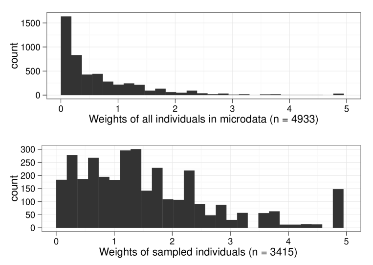
Figure 2: Histograms of original microdata weights (above) and sampled microdata after TRS integerisation (below) for a single area — zone 71 in the case study data.

3.6.3 Sample

As with the rounding approach, the truncation and replication stages alone are unable to produce microsimulated datasets of the correct size. The problem is exacerbated by the use of truncation instead of rounding: truncation is guaranteed to produce integer microdataset populations that are smaller, and in some cases much smaller than the actual (census) populations. In our case study, the simulated microdataset populations were around half the actual size populations defined by the census. This under-selection of whole cases has the following advantage: when using truncation there is no chance of over-sampling, avoiding the problem of simulated populations being slightly too large, as can occur with the threshold approach.

Given that the replication weights have already been included in steps 1 and 2, only the decimal weight remainders need to be included. This can be done using weighted random sampling without replacement. In R, the following function is used:

  sample(w, size=(pops[i,1] - pops[i,2]), prob= dr[,i])

Here, the argument ize \ within the \verb ample  command is set as the difference between the known population of each area (os[i,1] ) and the size obtained through the replication stage alone (os[i,2] ). The probability (rob ) of an individual being samled is determined by the decimal remainders. r \ varies between 0 an 1, as described above.

The results for one particular area are presented in Fig. 2. The distribution of selected individuals has shifted to the right, as the replication stage has replicated individuals as a function of their truncated weight. Individuals with low weights (below one) still constitute a large portion of those selected, yet these individuals are replicated fewer times. After TRS integerisation individuals with high decimal weights are relatively common. Before integerisation, individuals with IPF weights between 0 and 0.3 dominated. An individual-by-individual visualisation of the Monte Carlo sampling strategy is provided in Fig. 3. Comparing this with the same plot for the probabilistic methods (Fig. 1), the most noticeable difference is that the TRS and proportional probabilities approaches include individuals with very low weights. Another important difference is average point density, as illustrated by the transparency of the dots: in Fig. 1, there are shifts near the decimal weight threshold ($\sim$ 0.4 in this area) on the y-axis. In Fig. 3, by contrast, the transition is smoother: average darkness of single dots (the number of replications) gradually increases from 0 to 5 in both probabilistic methods.

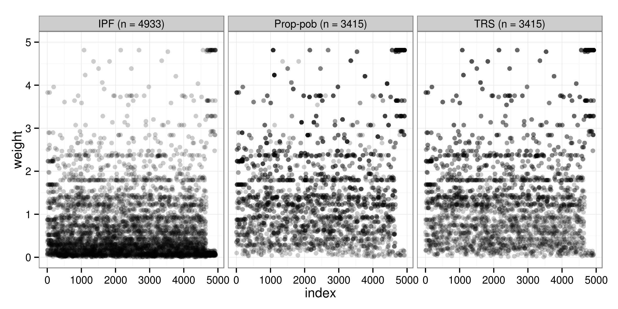
Figure 3: Overplotted scatter graphs of index against weight for the original IPF weights (left) and after proportional probabilities (middle) and TRS (right) integerisation for zone 71. Compare with Fig. 1.

Fig. 4 illustrates the mechanism by which the TRS sampling strategy works to select individuals. In the first stage (up to x = 1,717, in this case) there is a linear relationship between the indices of survey and sampled individuals, as the model iteratively moves through the individuals, replicating those with truncated weights greater than 0. This (deterministic) replication stage selects roughly half of the required population in our example dataset (this proportion varies from zone to zone). The next stage is probabilistic sampling (x = 1,718 onwards in Fig. 4): individuals are selected from the entire microdataset with selection probabilities equal to weight remainders.

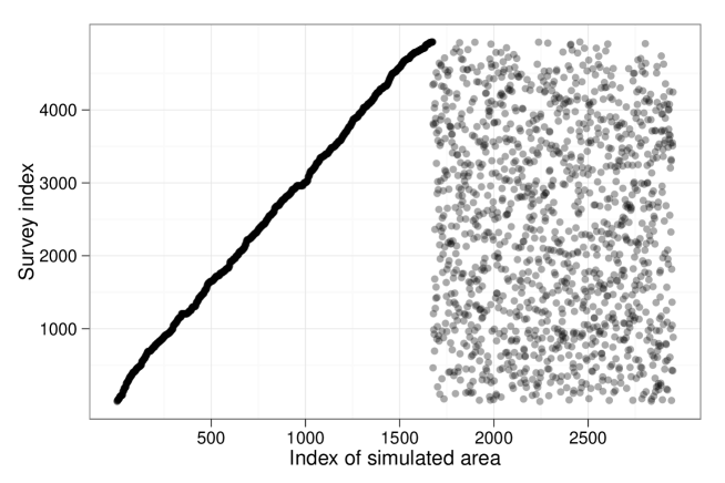
Figure 4: Scatter graph of the index values of individuals in the original sample and their indices following TRS Integerisation for a single area.

3.7 The test scenario: input data and IPF

The theory and methods presented above demonstrate how five integerisation methods work in abstract terms. But to compare them quantitatively a test scenario is needed. This example consists of a spatial microsimulation model that uses IPF to model the commuting and socio-demographic characteristics of economically active individuals in Sheffield. According to the 2001 Census, Sheffield has a working population of just over 230,000. The characteristics of these individuals were simulated by reweighting a synthetic microdataset based on aggregate constraint variables provided at the medium super output area (MSOA) level. The synthetic microdataset was created by ‘scrambling’ a subset of the Understanding Society dataset (USd). MSOAs contain on average just over 7,000 people each, of whom 44% are economically active in the study area; for the less sensitive aggregate constraints, real data were used. These variables are summarised in Table 3.

Table 3: Summary data for the spatial microsimulation model

	Aggregate data		Survey data
	71 zones, average pop.: 3077.5		4933 observations
Variable	N. categories	Most populous	Mean	Most populous
Age / sex	12	Male, 35 to 54 yrs	40.1	-
Mode	11	Car driver	-	Car driver
Distance	8	2 to 5 km	11.6	-
NS-SEC	9	Lower managerial	-	Lower managerial

The data contains both continuous (age, distance) and categorical (mode, NS-SEC) variables. In practice, all variables are converted into categorical variables for the purposes of IPF, however. To do this statistical bins are used. Table 3 illustrates similarities between aggregate and survey data overall (car drivers being the most popular mode of travel to work in both categories, for example). Large differences exist between individual zones and survey data, however: it is the role of iterative proportional fitting to apply weights to minimize these differences.

IPF was used to assign 71 weights to each of the 4,933 individuals, one weight for each zone. The fit between census and weighted microdata can be seen improving after constraining by each of the 40 variables (Fig. 5). The process is repeated until an adequate level of convergence is attained (see Fig. 6).

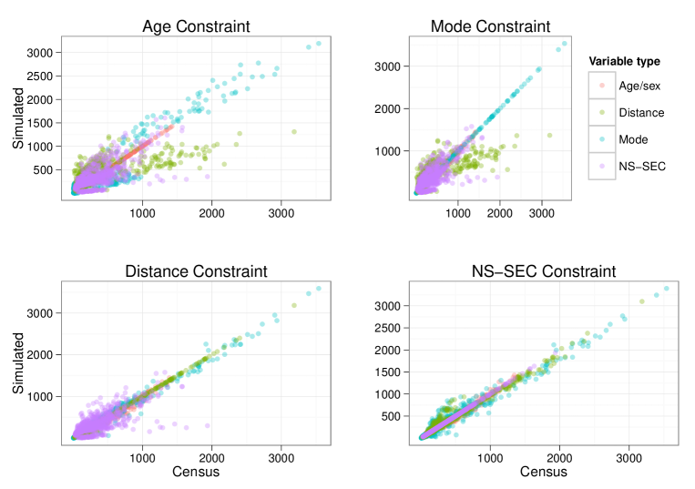
Figure 5: Visualisation of IPF method. The graphs show the iterative improvements in fit after age, mode, distance and finally NS-SEC constraints were applied (see Table 3). See footnote 4 for resources on how IPF works.

The weights were set to an initial value of one. The weights were then iteratively altered to match the aggregate (MSOA) level statistics, as described in Section 2.4.

Figure 6: Scatter graph illustrating the fit between census and simulated aggregates after 20 IPF iterations (compare with Fig. 5).

Four constraint variables link the aggregated census data to the survey, containing a total of 40 categories. To illustrate how IPF works, it is useful to inspect the fit between simulated and census aggregates before and after performing IPF for each constraint variable. Fig. 5 illustrates this process for each constraint. By contrast to existing approaches to visualising IPF (see Ballas et al., 2005c), Fig. 5 plots the results for all variables, one constraint at a time. This approach can highlight which constraint variables are particularly problematic. After 20 iterations (Fig. 6), one can see that distance and mode constraints are most problematic. This may be because both variables depend largely on geographical location, so are not captured well by UK-wide aggregates.

Fig. 5 also illustrates how IPF works: after reweighting for a particular constraint, the weights are forced to take values such that the aggregate statistics of the simulated microdataset match perfectly with the census aggregates, for all variables within the constraint in question. Aggregate values for the mode variables, for example, fit the census results perfectly after constraining by mode (top right panel in Fig. 5). Reweighting by the next constraint disrupts the fit imposed by the previous constraint — note the increase scatter of the (blue) mode variables after weights are constrained by distance (bottom left).

However, the disrupted fit is better than the original. This leads to a convergence of the weights such that the fit between simulated and known variables is optimised: Fig. 5 shows that accuracy increases after weights are constrained by each successive linking variable.

4 Results

This section compares the five previously describe approaches to integerisation — rounding, inclusion threshold, counter-weight, proportional probabilities and TRS methods. The results are based on the 20^th iteration of the IPF model described above. The following metrics of performance were assessed:

• Speed of calculation.

• Accuracy of results.

  • Sample size.

  • Total Absolute Error (TAE) of simulated areas.

  • Anomalies (aggregate cell values out by more than 5%).

  • Correlation between constraint variables in the census and microsimulated data.

Of these performance indicators accuracy is the most problematic. Options for measuring goodness-of-fit have proliferated in the last two decades, yet there is no consensus about which is most appropriate (Voas and Williamson, 2001). The approach taken here, therefore, is to use a range of measures, the most important of which are summarised in Table 4 and Fig. 7.

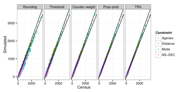
Figure 7: Scatterplots of actual (census) and simulated population totals for four integerisation techniques. The black lines represent 5% error in either direction.

4.1 Speed of calculation

The time taken for the integerisation of IPF weights was measured on an Intel Core i5 660 (3.33 GHz) machine with 4 Gb of RAM running Linux 3.0. The simple rounding method of integerisation was unsurprisingly the fastest, at 4 seconds. In second and third place respectively were the proportional probabilities and TRS approaches, which took a a couple of seconds longer for a single integerisation run for all areas. Slowest were the inclusion threshold and counter-weight techniques, which took three times longer than simple rounding. To ensure representative results for the probabilistic approaches, both were run 20 times and the result with the best fit was selected. These imputation loops took just under a minute.

The computational intensity of integerisation may be problematic when processing weights for very large datasets, or using older computers. However, the results must be placed in the context of the computational requirements of the IPF process itself. For the example described in Section 3.7, IPF took approximately 30 seconds per iteration and 5 minutes for the full 20 iterations.

4.2 Accuracy

In order to compare the fit between simulated microdata and the zonally aggregated linking variables that constrain them, the former must first be aggregated by zone. This aggregation stage allows the fit between linking variables to be compared directly (see Fig. 7). More formally, this aggregation allows goodness of fit to be calculated using a range of metrics (Williamson et al., 1998). We compared the accuracy of integerisation techniques using 5 metrics:

• Pearson’s product-moment correlation coefficient ($r$).

• Total and standardised absolute error (TAE and SAE),

• Proportion of simulated values falling beyond 5% of the actual values,

• The proportion of Z-scores significant at the 5% level.

• Size of the sampled populations,

The simplest way to evaluate the fit between simulated and census results was to use Pearson’s $r$, an established measure of association (Rodgers, 1988). The $r$ values for all constraints were 0.9911, 0.9960, 0.9978, 0.9989 and 0.9992 for rounding, threshold, counter-weight, proportional probabilities and TRS methods respectively. IPF alone had an $r$ value of 0.9996. These correlations establish an order of fit that can be compared to other metrics.

TAE and SAE are crude yet effective measures of overall model fit (Voas and Williamson, 2001). TAE has the additional advantage of being easily understood:

$$TAE=\sum\limits_{ij}|U_{ij}-T_{ij}|$$ (2)

where U and T are the observed and simulated values for each linking variable ($j$) and each area ($i$). SAE is the TAE divided by the total population of the study area. TAE is sensitive to the number of people within the model, while SAE is not. The latter is seen by Voas and Williamson (2001) as “marginally preferable” to the former: it allows cross-comparisons between models of different total populations (Kongmuang, 2006).

Table 4: Accuracy results for integerisation techniques.*

Method	Variables	TAE	SAE (%)	E $>$ 5% (%)	$Z{m}^{2}$ (%)
IPF	Age/sex	9	0.0	0.0	0.0
	Distance	4874	2.3	13.7	4.9
	Mode	4201	2.0	6.4	4.2
	NS-SEC	0	0.0	0.0	0.0
	All	9084	3.1	4.5	2.1
Round-	Age/sex	26812	12.5	81.5	39.8
ing	Distance	31981	14.9	80.1	65.1
	Mode	30558	14.2	81.4	48.9
	NS-SEC	27493	12.8	76.5	57.1
	All	116844	13.6	80.1	51.3
Thresh-	Age/sex	11076	5.1	49.2	8.1
old	Distance	27146	12.6	82.4	57.7
	Mode	14770	6.9	68.6	33.9
	NS-SEC	13770	6.4	55.2	24.1
	All	66762	7.8	62.5	28.7
Counter-	Age/sex	10242	4.8	47.7	6.6
weight	Distance	17103	8.0	70.2	39.3
	Mode	10072	4.7	60.4	21.6
	NS-SEC	11798	5.5	49.6	17.1
	All	49215	5.7	56.1	19.6
Propor-	Age/sex	9112	4.2	48.0	3.1
tional	Distance	8740	4.1	47.4	10.4
proba-	Mode	8664	4.0	60.8	9.0
bilities	NS-SEC	7778	3.6	37.6	3.3
	All	34294	4.0	49.0	6.2
TRS	Age/sex	5424	2.5	27.9	0.4
	Distance	10167	4.7	48.8	16.4
	Mode	7584	3.5	56.1	6.7
	NS-SEC	5687	2.6	24.9	1.1
	Total	28862	3.4	39.2	5.5

• * The probabilistic results represent the best fit (in terms of TAE) of 20 integerisation runs with the pseudo-random number seed set to 1000 for replicability — see Supplementary Information.

The proportion of values which fall beyond 5% of the actual values is a simple metric of the quality of the fit. It implies that getting a perfect fit is not the aim, and penalises fits that have a large number of outliers. The precise definition of ’outlier’ is somewhat arbitrary (one could just as well use 1%).

The final metric presented in Table 4 is based on the Z-statistic, a standardised measure of deviance from expected values, calculated for each cell of data. We use $Zm$, a modified version of the Z-statistic which is a robust measure of fit for each cell value Williamson et al. (1998). The measure of fit is appropriate here as it takes into account absolute, rather than just relative, differences between simulated and observed cell count:

$$Zm_{ij}=(r_{ij}-p_{ij})\Bigg{/}\left(\frac{p_{ij}(1-p_{ij}))}{\sum\limits_{ij}U_{ij}}\right)^{1/2}$$ (3)

where

$p_{ij}=\frac{U_{ij}}{\sum\limits_{ij}U_{ij}}\qquad and\qquad r_{ij}=\frac{T_{ij}}{\sum\limits_{ij}U_{ij}}$

To use the modified Z-statistic as a measure of overall model fit, one simply sums the squares of $zm$ to calculate $Z{m}^{2}$. This measure can handle observed cell counts below 5, which chi-squared tests cannot (Voas and Williamson, 2001).

The results presented in Table 4 confirm that all integerisation methods introduce some error. It is reassuring that the comparative accuracy is the same across all metrics. Total absolute error (TAE), the simplest goodness-of-fit metric, indicates that discrepancies between simulated and census data increase by a factor of 3.2 after TRS integerisation, compared with raw (fractional) IPF weights. Still, this is a major improvement on the simple rounding, threshold and counter-weight approaches to integerisation presented by Ballas et al. (2005a): these increased TAE by a factor of 13, 7 and 5 respectively. The improvement in fit relative to the proportional probabilities method is more modest. The proportional probabilities method increased TAE by a factor of 3.8, 23% more absolute error than TRS.

The differences between the simulated and actual populations ($Pop_{sim}-Pop_{cens}$) were also calculated for each area. The resulting differences are summarised in Table 5, which illustrates that the counter-weight and two probabilistic methods resulted in the correct population totals for every area. Simple rounding and threshold integerisation methods greatly underestimate and slightly overestimate the actual populations, respectively.

Table 5: Differences between census and simulated populations.

Metric	Rounding	Threshold	Others (CW, PP, TRS)
Mean	-372	8	0
Standard deviation	88	11	0
Max	-133	54	0
Min	-536	0	0
Oversample (%)	-13	0.3	0

5 Discussion and conclusions

The results show that TRS integerisation outperforms the other methods of integerisation tested in this paper. At the aggregate level, accuracy improves in the following order: simple rounding, inclusion threshold, counter-weight, proportional probabilities and, most accurately, TRS. This order of preference remains unchanged, regardless of which (from a selection of 5) measure of goodness-of-fit is used. These results concur with a finding derived from theory — that “deterministic rounding of the counts is not a satisfactory integerization” (Pritchard and Miller, 2012, p. 689). Proportional probability and TRS methods clearly provide more accurate alternatives.

An additional advantage of the probabilistic TRS and proportional probability methods is that correct population sizes are guaranteed. In terms of speed of calculation, TRS also performs well. TRS takes marginally more time than simple rounding and proportional probability methods, but is three times quicker than the threshold and counter-weight approaches. In practice, it seems that integerisation processing time is small relative to running IPF over several iterations. Another major benefit of these non-deterministic methods is that probability distributions of results can be generated, if the algorithms are run multiple times using unrelated pseudo-random numbers. Probabilistic methods could therefore enable the uncertainty introduced through integerisation to be investigated quantitatively (Beckman et al., 1996; Little and Rubin, ) and subsequently illustrated using error bars.

Overall the results indicate that TRS is superior to the deterministic methods on many levels and introduces less error than the proportional probabilities approach. We cannot claim that TRS is ‘the best’ integerisation strategy available though: there may be other solutions to the problem and different sets of test weights may generate different results. The issue will still present a challenge for future researchers considering the use of IPF to generate sample populations composed of whole individuals: whether to use deterministic or probabilistic methods is still an open question (some may favour deterministic methods that avoid psuedo-random numbers, to ensure reproducibility regardless of the software used), and the question of whether combinatorial optimisation algorithms perform better has not been addressed.

Our results provide insight into the advantages and disadvantages of five integerisation methods and guidance to researchers wishing to use IPF to generate integer weights: use TRS unless determinism is needed or until superior alternatives (e.g. real small area microdata) become available. Based on the code and example datasets provided in the Supplementary Information, we encourage others to use, build-on and improve TRS integerisation.

A broader issue raised by the this research, that requires further investigation before answers emerge, is ‘how do the integerised results of IPF compare with combinatorial optimisation approaches to spatial microsimulation?’ Studies have compared non-integer results of IPF with alternative approaches (Smith et al., 2009; Ryan et al., 2009; Rahman et al., 2010; Harland et al., 2012). However, these have so far failed to compare like with like: the integer results of combinatorial approaches are more useful (applicable to more types of analysis) than the non-integer results of IPF. TRS thus offers a way of ‘levelling the playing field’ whilst minimising the error introduced to the results of deterministic re-weighting through integerisation.

In conclusion, the integerisation methods presented in this paper make integer results accessible to those with a working knowledge of IPF. TRS outperforms previously published methods of integerisation. As such, the technique offers an attractive alternative to combinatorial optimisation approaches for applications that require whole individuals to be simulated based on aggregate data.

6 Acknowledgements

Thanks to: Mark Green, Luke Temple, David Anderson and Krystyna Koziol for proof reading and suggestions; to Eveline van Leeuwen for testing the methods on real data and improving the code; and to the anonymous reviewers for constructive comments. This research was funded by the Engineering and Physical Sciences Research council (EPSRC) the via the E-Futures Doctoral Training Centre.

References

- Anderson (2007) Anderson, B., 2007. Creating Small Area Income Estimates for England: spatial microsimulation modelling. Technical Report. University of Essex.
- Anderson (2013) Anderson, B., 2013. Estimating Small-Area Income Deprivation: An Iterative Proportional Fitting Approach, in: Tanton, R., Edwards, K. (Eds.), Spatial Microsimulation: A Reference Guide for Users. Springer Netherlands. volume 6 of Understanding Population Trends and Processes. chapter 4, pp. 49–67.
- Axhausen and Müller (2010) Axhausen, K., Müller, K., 2010. Population synthesis for microsimulation: State of the art. Technical Report August. Swiss Federal Institute of Technology Zurich.
- Ballas et al. (2005a) Ballas, D., Clarke, G., Dorling, D., Eyre, H., Thomas, B., Rossiter, D., 2005a. SimBritain: a spatial microsimulation approach to population dynamics. Population, Space and Place 11, 13–34.
- Ballas et al. (2006) Ballas, D., Clarke, G.P., Dewhurst, J., 2006. Modelling the Socio-economic Impacts of Major Job Loss or Gain at the Local Level: a Spatial Microsimulation Framework. Spatial Economic Analysis 1, 127–146.
- Ballas et al. (2005b) Ballas, D., Clarke, G.P., Wiemers, E., 2005b. Building a dynamic spatial microsimulation model for Ireland. Population, Space and Place 11, 157–172.
- Ballas et al. (2005c) Ballas, D., Dorling, D., Thomas, B., Rossiter, D., 2005c. Geography matters: simulating the local impacts of national social policies. Joseph Roundtree Foundation, York, UK.
- Ballas et al. (2013) Ballas, D., O’Donoghue, C., Clarke, G., Hynes, S., Morrissey, K., 2013. A Review of Microsimulation for Policy Analysis, Springer. chapter 3, p. 264.
- Beckman et al. (1996) Beckman, R., Baggerly, K., McKay, M., 1996. Creating synthetic baseline populations. Transportation Research Part A: Policy and Practice 30, 415–429.
- Birkin and Clarke (2012) Birkin, M., Clarke, G., 2012. The enhancement of spatial microsimulation models using geodemographics. The Annals of Regional Science 49, 515–532.
- Birkin and Clarke (1988) Birkin, M., Clarke, M., 1988. SYNTHESIS – a synthetic spatial information system for urban and regional analysis: methods and examples. Environment and Planning A 20, 1645–1671.
- Birkin and Clarke (1989) Birkin, M., Clarke, M., 1989. The Generation of Individual and Household Incomes at the Small Area Level using Synthesis. Regional Studies 23, 535–548.
- Birkin and Clarke (2011) Birkin, M., Clarke, M., 2011. Spatial Microsimulation Models: A Review and a Glimpse into the Future, in: Stillwell, J., Clarke, M., Stillwell, J. (Eds.), Population Dynamics and Projection Methods. Springer Netherlands. volume 4 of Understanding Population Trends and Processes, pp. 193–208.
- Bishop et al. (1975) Bishop, Y., Fienberg, S., Holland, P., 1975. Discrete Multivariate Analysis: theory and practice. MIT Press, Cambridge, Massachusettes.
- Clarke (1986) Clarke, M., 1986. Demographic processes and household dynamics: a microsimulation approach, in: Woods, R., Rees, P.H. (Eds.), Population Structures and Models: Developments in Spatial Demography, pp. 245–272.
- Deming (1940) Deming, W., 1940. On a least squares adjustment of a sampled frequency table when the expected marginal totals are known. The Annals of Mathematical Statistics .
- Edwards and Clarke (2009) Edwards, K.L., Clarke, G.P., 2009. The design and validation of a spatial microsimulation model of obesogenic environments for children in Leeds, UK: SimObesity. Social science & medicine 69, 1127–34.
- Fienberg (1970) Fienberg, S., 1970. An iterative procedure for estimation in contingency tables. The Annals of Mathematical Statistics 41, 907–917.
- Gentleman and Temple Lang (2007) Gentleman, R., Temple Lang, D., 2007. Statistical Analyses and Reproducible Research. Journal of Computational and Graphical Statistics 16, 1–23.
- Gilbert (2008) Gilbert, G.N., 2008. Agent-Based Models. Sage Publications, New York.
- Gilbert and Troitzsch (2005) Gilbert, N., Troitzsch, K.G., 2005. Simulation For The Social Scientist. McGraw-Hill International, New York.
- Goffe et al. (1994) Goffe, W.L., Ferrier, G.D., Rogers, J., 1994. Global optimization of statistical functions with simulated annealing. Journal of Econometrics 60, 65–99.
- Harland et al. (2012) Harland, K., Heppenstall, A., Smith, D., Birkin, M., 2012. Creating Realistic Synthetic Populations at Varying Spatial Scales: A Comparative Critique of Population Synthesis Techniques. Journal of Artificial Societies and Social Simulation 15, 1.
- Hermes and Poulsen (2012) Hermes, K., Poulsen, M., 2012. A review of current methods to generate synthetic spatial microdata using reweighting and future directions. Computers, Environment and Urban Systems 36, 281–290.
- Holm et al. (1996) Holm, E., Lindgren, U., Malmberg, G., Mäkilä, K., 1996. Simulating an entire nation, in: Clarke, G.P. (Ed.), Microsimulation for urban and regional policy analysis. Pion. number 6 in European research in regional science, pp. 164–186.
- Hooimeijer (1996) Hooimeijer, P., 1996. A life-course approach to urban dynamics: state of the art in and research design for the Netherlands, in: Clarke, G.P. (Ed.), Microsimulation for urban and regional policy analysis. Pion, London, pp. 28–63.
- Huang and Williamson (2001) Huang, Z., Williamson, P., 2001. The Creation of a National Set of Validated Small Area Population Microdata. Technical Report October. University of Liverpool.
- Hynes et al. (2009) Hynes, S., Morrissey, K., O’Donoghue, C., Clarke, G., 2009. A spatial micro-simulation analysis of methane emissions from Irish agriculture. Ecological Complexity 6, 135–146.
- Ince et al. (2012) Ince, D.C., Hatton, L., Graham-Cumming, J., 2012. The case for open computer programs. Nature 482, 485–8.
- Jiroušek and Přeučil (1995) Jiroušek, R., Přeučil, S., 1995. On the effective implementation of the iterative proportional fitting procedure. Computational Statistics & Data Analysis 19, 177–189.
- Johnston and Pattie (1993) Johnston, R.J., Pattie, C.J., 1993. Entropy-Maximizing and the Iterative Proportional Fitting Procedure. The Professional Geographer 45, 317–322.
- Kalantari et al. (2008) Kalantari, B., Lari, I., Ricca, F., Simeone, B., 2008. On the complexity of general matrix scaling and entropy minimization via the RAS algorithm. Mathematical Programming 112, 371–401.
- Kavroudakis et al. (2012) Kavroudakis, D., Ballas, D., Birkin, M., 2012. Using spatial microsimulation to model social and spatial inequalities in educational attainment. Applied Spatial Analysis and Policy , 1–23.
- Kongmuang (2006) Kongmuang, C., 2006. Modelling Crime: A Spatial Microsimulation Approach. Ph.D. thesis. University of Leeds.
- Lee (2009) Lee, A., 2009. Generating Synthetic Microdata from Published Marginal Tables and Confidentialised Files. Technical Report. Statistics New Zealand. Wellington.
- Li (2004) Li, Y., 2004. Samples of Anonymized Records (SARs) from the UK Censuses: A Unique Source for Social Science Research. Sociology 38, 553–572.
- (37) Little, R., Rubin, D., . Wiley Series in Probability and Statistics, New York. 1st edition.
- Miranti et al. (2010) Miranti, R., McNamara, J., Tanton, R., Harding, A., 2010. Poverty at the Local Level: National and Small Area Poverty Estimates by Family Type for Australia in 2006. Applied Spatial Analysis and Policy 4, 145–171.
- Mitchell et al. (2000) Mitchell, R., Shaw, M., Dorling, D., 2000. Inequalities in Life and Death: What If Britain Were More Equal? Policy Press, London.
- Mosteller (1968) Mosteller, F., 1968. Association and estimation in contingency tables. Journal of the American Statistical Association 63, 1–28.
- Norman (1999) Norman, P., 1999. Putting Iterative Proportional Fitting (IPF) on the Researcher’s Desk. Technical Report October. School of Geography, University of Leeds.
- Openshaw (1983) Openshaw, S., 1983. The modifiable areal unit problem. Geo Books, Norwich, UK.
- Peng et al. (2006) Peng, R.D., Dominici, F., Zeger, S.L., 2006. Reproducible epidemiologic research. American journal of epidemiology 163, 783–9.
- Pritchard and Miller (2012) Pritchard, D.R., Miller, E.J., 2012. Advances in population synthesis: fitting many attributes per agent and fitting to household and person margins simultaneously. Transportation 39, 685–704.
- R Core Team (2012) R Core Team, 2012. R: A Language and Environment for Statistical Computing. R Foundation for Statistical Computing. Vienna, Austria. ISBN 3-900051-07-0.
- Rahman et al. (2010) Rahman, A., Harding, A., Tanton, R., 2010. Methodological Issues in Spatial Microsimulation Modelling for Small Area Estimation. The international Journal of Microsimulation 3, 3–22.
- Rees et al. (2002) Rees, P., Martin, D., Williamson, P., 2002. Census data resources in the United Kingdom, in: Rees, P., Martin, D., Williamson, P. (Eds.), The census data system. Wiley, London. chapter 1.
- Rodgers (1988) Rodgers, J., 1988. Thirteen ways to look at the correlation coefficient. American Statistician 42, 59–66.
- Ryan et al. (2009) Ryan, J., Maoh, H., Kanaroglou, P., 2009. Population synthesis: Comparing the major techniques using a small, complete population of firms. Geographical Analysis 41, 181–203.
- Saito (1992) Saito, S., 1992. A multistep iterative proportional fitting procedure to estimate cohortwise interregional migration tables where only inconsistent marginals are known. Environment and Planning A 24, 1531–1547.
- Simpson and Tranmer (2005) Simpson, L., Tranmer, M., 2005. Combining sample and census data in small area estimates: iterative proportional fitting with standard software. The Professional Geographer 57, 222–234.
- Smith et al. (2009) Smith, D.M., Clarke, G.P., Harland, K., 2009. Improving the synthetic data generation process in spatial microsimulation models. Environment and Planning A 41, 1251–1268.
- Tanton and Edwards (2012) Tanton, R., Edwards, K., 2012. Spatial Microsimulation: A Reference Guide for Users. Springer, London.
- Tomintz et al. (2008) Tomintz, M.N.M., Clarke, G.P., Rigby, J.E.J., 2008. The geography of smoking in Leeds: estimating individual smoking rates and the implications for the location of stop smoking services. Area 40, 341–353.
- Vidyattama and Tanton (2010) Vidyattama, V.Y., Tanton, R., 2010. Projecting Small Area Statistics with Australian Spatial Microsimulation Model (SpatialMSM). Australasian Journal of Regional Studies 16, 99–120.
- Voas and Williamson (2000) Voas, D., Williamson, P., 2000. An evaluation of the combinatorial optimisation approach to the creation of synthetic microdata. International Journal of Population Geography 366, 349–366.
- Voas and Williamson (2001) Voas, D., Williamson, P., 2001. Evaluating Goodness-of-Fit Measures for Synthetic Microdata. Geographical and Environmental Modelling 5, 177–200.
- Williamson (2007) Williamson, P., 2007. CO Instruction Manual: Working Paper 2007/1 (v. 07.06.25). Technical Report June. University of Liverpool.
- Williamson et al. (1998) Williamson, P., Birkin, M., Rees, P.H., 1998. The estimation of population microdata by using data from small area statistics and samples of anonymised records. Environment and Planning A 30, 785–816.
- Williamson et al. (2002) Williamson, P., Mitchell, G., McDonald, A.T., 2002. Domestic Water Demand Forecasting: A Static Microsimulation Approach. Water and Environment Journal 16, 243–248.
- Wong (1992) Wong, D.W.S., 1992. The Reliability of Using the Iterative Proportional Fitting Procedure. The Professional Geographer 44, 340–348.
- Wu et al. (2008) Wu, B., Birkin, M., Rees, P., 2008. A spatial microsimulation model with student agents. Computers, Environment and Urban Systems 32, 440–453.
- Wu et al. (2010) Wu, B.M., Birkin, M.H., Rees, P.H., 2010. A Dynamic MSM With Agent Elements for Spatial Demographic Forecasting. Social Science Computer Review 29, 145–160.