Experimental observation of triple correlations
in fluids

Abstract

We present arguments for the hypothesis that under some conditions, triple correlations of density fluctuations in fluids can be detected experimentally by the method of molecular spectroscopy. These correlations manifest themselves in the form of the so-called 1.5- (i.e., sesquialteral) scattering. The latter is of most significance in the pre-asymptotic vicinity of the critical point and can be registered along certain thermodynamic paths. Its presence in the overall scattering pattern is demonstrated by our processing experimental data for the depolarization factor. Some consequences of these results are discussed.

Key words: density fluctuations, critical opalescence, 1.5-scattering, depolarization factor

PACS: 05.40, 05.70.Fh, 05.70.Jk, 64.70.Fx, 78.35.+c

Abstract

Наведено аргументи на користь гiпотези, що при певних умовах методом молекулярної спектроскопiї можна зареєструвати потрiйнi кореляцiї флуктуацiй густини в рiдинах. Цi кореляцiї проявляють себе у виглядi так званого 1.5- (тобто пiвторакратного) розсiяння, яке є найбiльш суттєвим в передасимптотичнiй областi критичної точки та може бути зареєстроване вздовж певних термодинамiчних шляхiв. Його присутнiсть у загальнiй картинi розсiяння демонструється результатами обробки вiдомих експериментальних даних для коефiцiєнта деполяризацiї. Обговорено деякi наслiдки цих результатiв.

Ключовi слова: флуктуацiї густини, критична опалесценцiя, розсiяння кратностi 1.5, коефiцiєнт деполяризацiї

1 Introduction

The intensity $I$ of light scattered by a one-component fluid drastically increases as the critical point is approached [1, 2]. The physical nature of this critical opalescence phenomenon is well-known, i.e., an increase in the magnitude of permittivity (in fact — density) fluctuations and the development of long-range correlations between them. The result is that $I$ is contributed to by not only single scattering effects, but also by those of higher multiplicities. One could expect that $I$ provides certain information about higher-order correlation functions for the density fluctuations.

However, a common view is that it is only double scattering [3, 4, 5, 6, 7, 8] together, probably, with Andreev’s scattering (due to fluctuations in the distribution function of thermal fluctuations) [9, 10, 11] and triple scattering [12] that contribute significantly near the critical point. The pertinent theories are based upon quasi-Gaussian statistics for the fluctuations. As a consequence, any information on the irreducible parts of higher-order correlation functions is lost and multiple scattering is viewed as parasitic.

By contrast, we pursue the idea that the so-called 1.5- (sesquialteral) scattering, caused by triple correlations of density fluctuations, contributes significantly to $I$. In this report, we support this statement by our results of processing extensive experimental data [13] on the depolarization factor near the critical point. In our view, these results strongly indicate that the 1.5-scattering is noticeably present, under certain conditions, in the overall scattering pattern. Moreover, the idea of 1.5-scattering allows us to give simple explanations for the anomalies in the behavior of $I^{-1}$ in the gravity field [14, 15] and those of the Landau-Plazcek ratio near the $\lambda$-line [16, 17, 18], which were observed long ago, but have been interpreted controversially.

It is also important to note that, according to our own theory and in view of earlier estimates [4], from among different three-point configurations of density fluctuations $\delta\rho$ (located at points ${\bf r}$, ${\bf r}_{1}$, and ${\bf r}^{\prime}$), the major contribution to the integrated 1.5-scattering intensity $I_{1.5}$ is made by those in which two successively scattering fluctuations merge on the macroscopic scale ($|{\bf r}-{\bf r}_{1}|\to 0$; technically, this is a consequence of the replacement of the internal electromagnetic field propagators in the iterative series for the scattered field with their leading short-range singularities). As a result, $I_{1.5}$ is determined by the Fourier transform of the pair correlation function $\langle\left[\delta\rho(\rm{\bf r})\right]^{2}\delta\rho({\bf r}^{\prime})\rangle$. Provided Polyakov’s hypothesis [19] (see also [20, 21]) of conformal symmetry of critical fluctuations is valid, the latter is expected to vanish at the critical point (see appendix A). It follows that the recovery of the 1.5-scattering contribution from $I$ and a scrutinized study of its behavior along appropriate thermodynamic paths ending up at the critical point provide a unique opportunity for experimental verification of Polyakov’s hypothesis [19] for systems with scalar order parameters.

2 Theory of 1.5-scattering

2.1 General expression

The theory of 1.5-scattering was proposed in [22] and developed further in [23, 24]; some additional numerical estimates were made in [25, 26]. We assume that molecular light scattering from condensed matter is a result of re-emission of light not only by single fluctuations, but also by compact groups of fluctuations. By compact we understand any group of fluctuations all the distances between which are much shorter than the wavelength $\lambda$ of the probing light in the medium. Physically, scattering by such a group is single. The overall polarized single-scattering spectrum is, therefore, given by the series [23]

$$I({\rm{\bf q}},\omega)={\sum\limits_{n,m\geqslant 1}{I_{nm}({\rm{\bf q}},\Omega)}},$$ (2.1)

where

$$I_{nm}({\rm{\bf q}},\Omega)\propto\,\left({-{\frac{{1}}{{3\varepsilon_{0}}}}}\right)^{n+m-2}\times{\frac{{1}}{{\pi}}}\mathop{\symoperators Re}\nolimits{\int\limits_{0}^{+\infty}{{\rm d}t}}{\int\limits_{V}{\rm d}{\rm{\bf r}}{\left\langle{\left[{\delta\varepsilon({\rm{\bf r}},t)}\right]^{n}\left[{\delta\varepsilon(0,0)}\right]^{m}}\right\rangle}\,{\rm e}^{{\rm i}\Omega t-\mathrm{i}{\rm{\bf q}}\cdot{\rm{\bf r}}}}$$ (2.2)

is the contribution from a pair of compact groups of $n$ and $m$ permittivity fluctuations [attributed further to density fluctuations, $\delta\varepsilon\approx\left(\partial\varepsilon/\partial\rho\right)_{T}\delta\rho$], $\varepsilon_{0}$ is the equilibrium value of the permittivity, $\Omega$ and ${\rm{\bf q}}$ are the changes in the light frequency and wavevector due to scattering, and the scattering volume $V$ is included into the proportionality coefficient.

It is only the term $I_{11}({\rm{\bf q}},\Omega)$ in equation (2.1) that has been associated so far with the single scattering. The 1.5-scattering intensity is defined as $I_{1.5}({\rm{\bf q}},\Omega)=I_{12}({\rm{\bf q}},\Omega)+I_{21}({\rm{\bf q}},\Omega)$.

2.2 Hydrodynamic region, $qr_{\mathrm{c}}\ll 1$

Far enough from the critical point, where the correlation radius $r_{\mathrm{c}}\ll\lambda$ and nonlocal correlations between fluctuations can be ignored, the integrated 1.5-scattering intensity can be expressed in terms of the third moment of thermodynamic density fluctuations $\Delta\rho$ [22]:

$$I_{1.5}\propto-\frac{2}{3\varepsilon_{0}}\left(\frac{\partial\varepsilon}{\partial\rho}\right)^{3}\widetilde{V}\langle(\Delta\rho)^{3}\rangle=-\frac{2}{3\varepsilon_{0}}\left(\rho\frac{\partial\varepsilon}{\partial\rho}\right)^{3}\frac{k^{2}_{\mathrm{B}}T^{2}}{\widetilde{V}}\left[2\beta_{T}^{2}+\left(\frac{\partial\beta_{T}}{\partial P}\right)_{T,V}\right],$$ (2.3)

where $\beta_{T}$ is the isothermal compressibility of the fluid and $\widetilde{V}$ is a macroscopic volume over which the fluctuations $\delta\rho$ are averaged to single out their thermodynamic parts $\Delta\rho$. We suggest that $\widetilde{V}$ is slightly dependent on temperature far away from the critical point, but $\widetilde{V}\propto r_{\mathrm{c}}^{3}\propto\beta_{T}^{3/2}$ in the critical region.

Calculations with the van der Waals and Dieterici equations of states give the estimates

$$I_{1.5}\propto-\frac{1}{\varepsilon_{0}}\left(\rho\frac{\partial\varepsilon}{\partial\rho}\right)^{3}\frac{k^{2}_{\mathrm{B}}T^{2}}{\widetilde{V}}\cdot 6P_{c}\omega\beta_{T}^{3}$$

and

$$I_{1.5}\propto-\frac{2}{3\varepsilon_{0}}\left(\rho\frac{\partial\varepsilon}{\partial\rho}\right)^{3}\frac{k^{2}_{\mathrm{B}}T^{2}}{\widetilde{V}}\cdot\left(\beta_{T}^{2}+4P_{\mathrm{c}}\omega\beta_{T}^{3}\right),$$

respectively, where $\omega\equiv\rho_{\mathrm{c}}/\rho-1$, $|\omega|\ll 1$ is the deviation of $\rho$ from the critical value $\rho_{\mathrm{c}}$ and $P_{\mathrm{c}}$ is the critical pressure. It follows that the 1.5-scattering can become of significance in those domains in the $(\tau,\omega)$-plane where $\omega\neq 0$, but $\beta_{T}$ is sufficiently large. Then, $I_{1.5}\propto\omega\beta_{T}^{3/2}$ for a non-critical isochore, but $I_{1.5}\propto\beta_{T}^{1/2}$ or even $I_{1.5}\to 0$ for the critical one.

A distinctive feature of the 1.5-scattering contribution is that it is not positive definite: for instance, $I_{1.5}<0$ in the region where $\omega>0$ and $\tau>0$, at least.

2.3 Fluctuation region, $qr_{\mathrm{c}}\gg 1$

Understanding, in this section, $\rho$ as a scalar order parameter, we see that formulas (2.1) and (2.2) agree with the hypothesis of algebra of fluctuating quantities [20]. Then, within the first order of $\epsilon$-expansion and in the long-wave limit $q\to 0$, the critical index of $I_{1.5}$, defined by $I_{1.5}\propto|\tau|^{-\mu_{21}}$, is estimated to be $\mu_{21}\approx 0.67$ for $\omega=0$ [22]. This value is close to an earlier estimate of 0.7 given in [20]. Correspondingly, $I_{1.5}\propto\beta_{T}^{1/2}$ on the critical isochore and in the immediate vicinity of the critical point.

This result can be refined using the algebra of fluctuating quantities (see appendix A). However, it is more important to emphasize that it disregards the conformal invariance hypothesis [19]. If the latter is indeed valid, then the orthogonality relation holds for fluctuating quantities with different scaling dimensions (see [20, 21]), that is, $I_{1.5}\to 0$ as the critical point is approached.

2.4 Intermediate region, $qr_{\mathrm{c}}\lesssim 1$

This region is of special interest to us because it is typical of actual experiment. Taking into account that correlations between fluctuations $\delta\rho$ remain relatively weak, we argue [23] that the convolution-type approximation

$${\left\langle{\rho_{{\rm{\bf k}}_{1}}\rho_{{\rm{\bf k}}_{2}}\rho_{{\rm{\bf k}}_{3}}}\right\rangle}\approx-{\frac{{2{c}^{\prime}}}{{k_{B}T\sqrt{V}}}}G(k_{1})G(k_{2})G(k_{3})\,\delta_{{\rm{\bf k}}_{3},-{\rm{\bf k}}_{1}-{\rm{\bf k}}_{2}}$$

can be used for the three-point correlation function of density fluctuations. Here, $\rho_{{\rm{\bf k}}}$ is the Fourier component of $\delta\rho({\rm{\bf r}})$, $G(k)\equiv\langle{|\rho_{{\rm{\bf k}}}|^{2}\rangle}$, and ${c}^{\prime}$ is a $\bf k$-independent function of temperature and density. Calculations with the Ornstein-Zernike expression for $G(k)$ then give:

$$I_{1.5}(q)\propto\frac{c^{\prime}}{3\pi\varepsilon_{0}}\left(\rho\frac{\partial\varepsilon}{\partial\rho}\right)^{3}\frac{\rho^{3}k^{2}_{\mathrm{B}}T^{2}\beta_{T}^{3}}{qr_{\mathrm{c}}^{4}\left(1+q^{2}r_{\mathrm{c}}^{2}\right)}\arctan\left(\frac{qr_{\mathrm{c}}}{2}\right).$$ (2.4)

Requiring that in the limit $qr_{\mathrm{c}}\ll 1$, equation (2.4) transforms into equation (2.3), we recover ${c}^{\prime}$ through the third thermodynamic moment of density fluctuations, with an accuracy to a positive proportionality constant:

$$c^{\prime}\propto-\left[2\beta_{T}^{2}+\left(\frac{\partial\beta_{T}}{\partial P}\right)_{T,V}\right]\left(\rho\beta_{T}\right)^{-3}.$$ (2.5)

Extrapolation of formulas (2.4) and (2.5) on the fluctuation region shows that (see appendix B) $c^{\prime}\to 0$ and, therefore, $I_{1.5}\to 0$ as both $\tau\to 0$ and $\omega\to 0$, which is in accordance with the conformal invariance hypothesis.

The structure of the 1.5-scattering spectrum in the intermediate region is discussed in [24].

3 Depolarization factor

3.1 Theoretical considerations

Now, we are in a position to scrutinize the effect of 1.5-scattering on the depolarization factor $\Delta$ as a function of temperature (in fact, $\beta_{T}$) and the geometrical size $L\sim V^{1/3}$ (volume $V$) of the scattering system. Suppose that the following contributions to $I$ are present in the intermediate region $qr\lesssim 1$: (1) the ‘‘standard’’ intensity $I_{11}\propto V\beta_{T}$ of polarized single scattering due to density fluctuations [1, 2]; (2) the intensity $I_{1.5}$ of polarized 1.5-scattering [22, 23, 24]; (3) the intensity $I_{\rm a}\propto V$ of depolarized single scattering due to anisotropy fluctuations [1] (it is virtually insensitive to the critical point); (4) the intensity $I_{2\rm p}\propto V^{4/3}\beta_{T}^{2}$ of polarized double scattering due to density fluctuations [3, 4, 5, 6, 7, 8]; (5) the intensity $I_{2\rm d}\propto V^{4/3}\beta_{T}^{2}$ of depolarized double scattering due to density fluctuations [3, 4, 5, 6, 7, 8]; (6) the intensity $I_{\rm A}\propto V\beta_{T}^{1/2}$ of depolarized single scattering due to fluctuations in the distribution function of thermal fluctuations (Andreev’s scattering) [9]. Then, $\Delta$ is given by

$$\Delta=\frac{I_{\rm a}+I_{2\rm d}+I_{\rm A}}{I_{1}+I_{1.5}+I_{2\rm p}}\,.$$ (3.1)

In view of the individual temperature dependences of the above contributions and under the condition $I_{1.5}=0$, $\Delta$ as a function of $\beta_{T}$ is expected to decrease first, then reach a minimum, and then increase again. Such a behavior, indeed observed in the experiment, is considered as a manifestation of double scattering effects. However, as we show later, the presence of the 1.5-scattering contribution does not alter this qualitative behavior of $\Delta$ as a function of $\beta_{T}$.

Thus, expression (3.1) should be transformed in order to obtain an experimentally-measurable function whose behavior significantly depends on whether the 1.5-scattering contributes to $\Delta$ or not [22]. Rewriting (3.1) as

$$\frac{I_{2\rm d}}{I_{1}\Delta}=\frac{1+I_{1.5}I_{1}^{-1}+I_{2\rm p}I_{1}^{-1}}{1+I_{\rm a}I_{2\rm d}^{-1}+I_{\rm A}I_{2\rm d}^{-1}}$$ (3.2)

and taking into account the specific features of the intensity contributions, we immediately arrive at the relation

$$\frac{L\beta_{T}}{\Delta}\propto\frac{1+a\beta_{T}^{1/2}+bL\beta_{T}}{1+cL^{-1}\beta_{T}^{-2}+dL^{-1}\beta_{T}^{-3/2}}$$ (3.3)

valid for the intermediate region $qr\lesssim 1$. Here, the coefficients $b$, $c$, and $d$ are practically temperature-independent and positive constants. The coefficient $a\propto c^{\prime}\arctan\left(\frac{qr_{\mathrm{c}}}{2}\right)/r_{\mathrm{c}}$ is due to the 1.5-scattering contribution and is not positive definite. If the 1.5-scattering is negligible, then $a=0$ and the right-hand side in formula (3.3) is a monotonous increasing function of $\beta_{T}$. With the 1.5-scattering present, this monotonous behavior is expected to be violated. The effect should be most pronounced in the following two cases.

(1) The critical point is approached along a noncritical isochore $\omega>0$. Then, $I_{1.5}\propto-\beta_{T}^{3/2}$ and $a$ is close to a negative constant.

(2) The critical point is approached along the path where $\tau\to 0$, $\omega\to 0$, and $I_{1.5}>0$. The relative magnitude $I_{1.5}/I_{1}$ of the 1.5-scattering should start decreasing somewhere due to the temperature law $I_{1.5}\propto\beta_{T}^{1/2}$ coming into play [20, 22] (see section 2.3) or as a consequence of the conformal invariance [19, 20]. As such a path, the liquid branch of the coexistence curve can be quoted.

Thus, by varying the temperature ($\beta_{T}$) and density ($\omega$) of the scattering system, we hope to ‘‘stick out’’ the 1.5-scattering contribution from among the others. It should manifest itself as a non-monotonous behavior of the experimentally-measurable quantity $L\beta_{T}/\Delta^{-1}$ with $\beta_{T}$. The fact that the scattering contributions involved depend differently on $L$, provides an additional powerful option for analysis. Some results obtained by processing the extensive depolarization factor data [13] are presented in figures 1–12. They generalize our earlier results [25].

3.2 Data processing

3.2.1 Noncritical isochores $\rho<\rho_{\mathrm{c}}$, $\tau>0$

Figure 1 represents the log-linear plots of the quantity $L(D\Delta)^{-1}\propto L\beta_{T}\Delta^{-1}$ as a function of the parameter ($k_{0}$ is the wavevector in vacuum of the incident light)

$$D^{-1}=\frac{k_{0}^{4}}{144\pi^{2}}\left(\varepsilon_{0}-1\right)^{2}\left(\varepsilon_{0}+2\right)^{2}k_{\rm B}T\beta_{T}\propto\beta_{T}$$

for xenon along the $\omega=6.8\times 10^{-3}$ isochore and five values of $L$ (in cm). The parameter $D$ (in m) is a convenient measure of the distance to the critical point [27]. It is evaluated in [13] as a function of temperature and density by using the Clausius-Mossotti relation for $\varepsilon_{0}$ and the restricted linear model equation of state [28] for $\beta_{T}$. These calculations are claimed to be most reliable for the region not very close to and not far away from the critical point, i.e., the one of special interest to us.

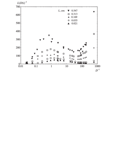
Figure 1: $L(D\Delta)^{-1}$ versus $D^{-1}$ along the $\omega=6.8\times 10^{-3}$ isochore of xenon for five values of $L$, based on experimental data [13]. From left to right, $\tau$ decreases from $7.8\times 10^{-2}$ to $1.2\times 10^{-5}$. Three segments can be distinguished on each of these log-linear plots.

As $\tau$ reduces from $7.8\times 10^{-2}$ to $1.2\times 10^{-5}$, three typical temperature intervals are clearly seen in figure 1. We shall refer to them as segments A (leftmost), B (central) and C (rightmost). It is easy to note that simple division of $L(D\Delta)^{-1}$ by $L$ and changing to $(D\Delta)^{-1}$ as a function of $D^{-1}$ for different values of $L$ transforms the original plots dissimilarly on these segments: the plots tend to merge on A and C, but invert the vertical ordering and disperse on B (figure 3). This fact implies that $(D\Delta)^{-1}$ is contributed to by terms with differing functional dependences on $L$. Our further analysis of them is guided by relation (3.3).

Figure 2: $(D\Delta)^{-1}$ versus $D^{-1}$ for the data shown in figure 1.

Figure 3: $(D\Delta)$ versus $D^{2}$ for segments A. From right to left, $\tau$ decreases from $7.8\times 10^{-2}$ to $3.3\times 10^{-3}$.

Suppose that on segments A, i.e., the most distant from the critical point, $I_{1}$ prevails much over $I_{1.5}$ and $I_{2\rm p}$. Then, relation (3.3) takes the form

$$\frac{L\beta_{T}}{\Delta}\propto\frac{1}{1+cL^{-1}\beta_{T}^{-2}+dL^{-1}\beta_{T}^{-3/2}}\,.$$

It follows that the dependence of $(D\Delta)$ upon $D^{2}$ should be close to a linear one, with the slope independent of $L$ and, if the Andreev contribution is noticeable, a slight concavity: $(D\Delta)\propto{\rm const}+cD^{2}+d(D^{2})^{3/4}.$ Figure 3 does exhibit, at least approximately, such kind of dependence. The study of the latter could, in principle, provide experimental estimates for the magnitude of $I_{\rm A}$. However, the discussion of this issue is beyond the scope of the present report.

On segments B, where we expect $I_{2\rm d}$ to dominate over $I_{\rm a}$ and $I_{\rm A}$, but $I_{2\rm p}$ to remain relatively weak as compared to $I_{1}$ and $I_{1.5}$, relation (3.3) takes the form

$$\frac{L\beta_{T}}{\Delta}\propto{1+a\beta_{T}^{1/2}}.$$

At $\omega>0$, $L(D\Delta)^{-1}$ should decrease with $D^{-1/2}$ by the linear law $L(D\Delta)^{-1}\propto-D^{-1/2}$, with negative and equal slopes for different values of $L$ (figures 5 and 5). Correspondingly, the dependences of $(D\Delta)^{-1}$ upon $-D^{-1/2}$ should be linear on B, with slopes inversely proportional to $L$, but, as was already mentioned, merge on A (figure 6).

Figure 4: $L(D\Delta)^{-1}$ versus $D^{-1/2}$ for segments A and B. From left to right, $\tau$ decreases from $7.8\times 10^{-2}$ to $1.4\times 10^{-4}$.

Figure 5: $L(D\Delta)^{-1}$ versus $D^{-1/2}$ for the portions of segments B where $\tau$ decreases from $9.8\times 10^{-4}$ to $1.4\times 10^{-4}$.

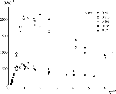
Figure 6: $(D\Delta)^{-1}$ versus $D^{-1/2}$ for the data shown in figure 5.

Finally, segments C are formed mainly by single and true double scatterings. Relation (3.3) takes the form

$$\frac{L\beta_{T}}{\Delta}\propto 1+bL\beta_{T}$$

and we expect $L(D\Delta)^{-1}$ to increase with $D^{-1}$ by a linear law, with slope proportional to $L$ (figure 8). The $(D\Delta)^{-1}$ versus $D^{-1}$ plots for different values of $L$ should approach a single straight segment as $D^{-1}$ increases (figure 8).

Figure 7: $L(D\Delta)^{-1}$ versus $D^{-1}$ for the entire $\omega=6.8\times 10^{-3}$ data plotted with a linear $D^{-1}$ scale. Segments C stand out as $\tau$ decreases rightwards from $8.6\times 10^{-5}$ to $1.2\times 10^{-5}$.

Figure 8: $(D\Delta)^{-1}$ versus $D^{-1}$ for the entire $\omega=6.8\times 10^{-3}$ data plotted with a linear $D^{-1}$ scale.

Figure 9: $L(D\Delta)^{-1}$ versus $D^{-1}$ along the liquid branch of the coexistence curve of xenon; $L=0.547\,{\rm cm}$. From left to right, $\tau$ changes from $-9.2\times 10^{-2}$ to $-2.9\times 10^{-5}$.

3.2.2 Liquid branch of the coexistence curve

The dependence of $L(D\Delta)^{-1}$ upon $D^{-1}$ along the liquid branch of the coexistence curve of xenon is shown in figure 9. It agrees well with our expectations.

Thus, the above processing of experimental data [13] clearly reveals the presence in the overall scattering pattern of a contribution which we associate with the 1.5- (sesquialteral) molecular light scattering.

3.3 Numerical estimates

Now, we present quantitative estimates of the magnitude of 1.5-scattering intensity. They were obtained by fitting the $L(D\Delta)^{-1}$ versus $D^{-1}$ data for the entire $\omega=6.8\times 10^{-3}$ isochore and then used to reproduce the original $\Delta$ versus $D$ data [13].

In view of formulas (3.2) and (3.3), the fitting function was taken in the form

$$f(x)=\frac{x^{2}}{C+x^{2}}\left(K+Ax^{1/2}+Bx\right),\qquad x\equiv D^{-1},$$

and the following two sets of coefficients were chosen: $K_{1}=581.066$, $A_{1}=-63.6968$, $B_{1}=3.66569$, $C_{1}=0.012$ and $K_{2}=607.508$, $A_{2}=-89.0932$, $B_{2}=5.79532$, $C_{2}=0.012$. The relative magnitudes $r_{1.5}\equiv{I_{1.5}}/{I_{1}}$ and $r_{2{\rm p}}\equiv{I_{2{\rm p}}}/{I_{1}}$ of the 1.5-scattering and polarized double scattering, as compared to the single scattering, were estimated as

$$r_{1.5}=\frac{Ax^{1/2}}{K}\,,\qquad r_{2{\rm p}}=\frac{Bx}{K}\,.$$

To calculate $\Delta$ with $f_{i}$, our theoretical estimate [11] $I_{2\rm d}\approx\frac{1}{8}I_{2\rm p}$ was additionally used. Then,

$$\Delta=\frac{Bx}{8Kf(x)}\,.$$

Figure 10: Fitting the $(D\Delta)^{-1}$ versus $D^{-1}$ data ($\omega=6.8\times 10^{-3}$, $L=0.547\,{\rm cm}$) with $f_{1}$ (dashed line) and $f_{2}$ (solid line).

Figure 11: Fitting the $\Delta$ versus $D$ data ($\omega=6.8\times 10^{-3}$, $L=0.547\,{\rm cm}$) with $f_{1}$ (dashed line) and $f_{2}$ (solid line).

The results are demonstrated by figures 11–12. They clearly show that in the intermediate region, the intensities $I_{1.5}$ and $I_{2{\rm p}}$ reach magnitudes comparable with that of $I_{1}$, but are opposite in sign and tend to compensate for each other. These facts are surprising. They contradict the common view that multiple scattering contributions come into play gradually as the critical point is approached. In other words, they imply an asymptotic nature of the iterative series for the overall scattering intensity near the critical point. They can also be interpreted in the sense that triple and quadruple correlations in fluids contribute, at least to light scattering effects, in opposite directions.

The agreement of our fitting results with the $\Delta$-data [13] (figure 11) is also unexpectedly good.

Figure 12: $I_{1.5}/I_{1}$, $I_{2{\rm{p}}}/I_{1}$, and $\left(I_{1.5}+I_{2{\rm p}}\right)/I_{1}$ along the $\omega=6.8\times 10^{-3}$ isochore of xenon, $L=0.547\,{\rm cm}$, as estimated with $f_{1}$ (dashed line) and $f_{2}$ (solid line).

4 Conclusion

The above estimates have prompted us to identify other experiments where the situation is favorable for 1.5-scattering to come into play. First of all, of interest are the studies on light scattering from critical fluids under the earth’s gravity. Due to the gravity effect, the system is spatially inhomogeneous in the vertical direction. A negative 1.5-contribution is expected to appear in the light scattered from the fluid layers located above the level of critical density. For such a layer, the total scattering intensity $I$ should, as a function of temperature, start decreasing somewhere as the critical point is approached. In other words, the $I^{-1}$ versus $\tau$ dependence should have a minimum at some $\tau_{0}$. The effect was indeed registered, for instance, in freon 113 [14, 15]. Our estimations for the minimum location, $\tau_{0}\sim 10^{-3}$ for heights up to $20\,{\rm mm}$ ($\tau>0$), agree well with experiment.

We suggest that a specially-designed processing of the gravity-induced height- and temperature dependences of $I$, obtained for systems with a scalar order parameter, is a feasible opportunity for singling out the 1.5-scattering contribution and verifying Polyakov’s conformal invariance hypothesis.

To finish, we mention that the studies of the spectral distribution in critical opalescence spectra are of great interest as well. In particular, we have proved that in the presence of 1.5- and double scattering effects, the ratio of the integrated intensities of the Rayleigh and Brillouin components takes the form

$$R_{{\rm exp}}=R\frac{1+a_{1.5}r_{1.5}+a_{2{\rm p}}r_{{2{\rm p}}}}{1+b_{1.5}r_{1.5}+b_{2{\rm p}}r_{2{\rm p}}}\,,$$ (4.1)

where $R=\gamma-1$ is the well-known Landau-Placzek ratio [30] for single scattering ($\gamma\equiv c_{P}/c_{V}$, $c_{P}$ and $c_{V}$ being the specific heats at constant pressure and volumes). The coefficients $a_{1.5}$ and $b_{1.5}$ are given in [24], whereas $a_{2{\rm p}}$ and $b_{2{\rm p}}$ can be recovered from the results [31]:

$$a_{2{\rm p}}=1-\frac{3}{2\gamma}+\frac{1}{2(\gamma-1)}\,,\qquad b_{2{\rm p}}=2-\frac{3}{2\gamma}\,.$$ (4.2)

Suggesting that $r_{1.5}=0$, it is not difficult to verify, based on experimental data [32] for ${\rm He}^{4}$, that the double scattering alone should cause $R_{{\rm exp}}$ to exceed $R$ as the $\lambda$-line is approached along a high-pressure isobar. Such a fact was indeed registered [18], but in most other experiments in this series the tendency was direct opposite [16, 17, 18]. We attribute the reduction in $R_{{\rm exp}}$ to the effect of 1.5-scattering.

Our detailed calculations of the above effects will be presented elsewhere.

Appendix A

Let $A_{k}({\bf r})$ be a complete set (algebra) of fluctuating scalar quantities with scaling dimensions $\Delta_{k}$: under the scaling transformations ${\bf r}\rightarrow\lambda{\bf r}$, $A_{k}(\lambda{\bf r})\rightarrow\lambda^{-\Delta_{k}}A_{k}({\bf r})$. According to the local algebra hypothesis (see, for instance, [20]), the scalar function $\delta\rho({\bf r})$ and, therefore, the scalar function $\left[\delta\rho({\bf r})\right]^{2}$ can be developed into the series

$$\delta\rho({\bf r})=\sum_{k=1}^{\infty}a_{k}A_{k}({\bf r}),\qquad\left[\delta\rho({\bf r})\right]^{2}=\sum_{m,n=1}^{\infty}b_{mn}B_{mn}({\bf r}),$$

where the coefficients $b_{mn}$ are simply related to the coefficients $a_{k}$, and $B_{mn}({\bf r})=A_{m}({\bf r})A_{n}({\bf r})$ are scalar quantities with definite scaling dimensions $\Delta_{mn}=\Delta_{m}+\Delta_{n}$: $B_{mn}(\lambda{\bf r})\rightarrow\lambda^{-\Delta_{mn}}B_{mn}({\bf r})$. Correspondingly, the pair correlation function $\langle\delta\rho({\bf r}^{\prime})\left[\delta\rho(\rm{\bf r})\right]^{2}\rangle$ is given by a linear combination of pair correlators $K_{k,mn}(|{\bf r}^{\prime}-{\bf r}|)\equiv\langle A_{k}({\bf r}^{\prime})B_{mn}({\bf r})\rangle$.

For a $d$-dimensional system with scalar order parameter, only the Fourier transforms of those $K_{k,mn}$ can reveal a singular behavior near the critical point which satisfy the condition $\Delta_{k}+\Delta_{mn}<d$. In the first-order $\epsilon$-expansion $\Delta_{k}=\frac{1}{2}k(2-\epsilon)+\frac{1}{6}k(k-1)\epsilon$, where $\epsilon=4-d$ [20]. If $d=3$, then the relevant correlators are $K_{1,11}$, $K_{1,12}=K_{1,12}$, and $K_{2,11}$, each involving two scalar quantities with different scaling dimensions. Once Polyakov’s conformal symmetry hypothesis holds true and the system is spatially homogeneous and isotropic, they all vanish at the critical point due to the orthogonality relation (see [20, 21] and the literature cited therein).

Appendix B

As one of the ways for evaluating $c^{\prime}$ in the fluctuation region, we can use the asymptotic equation of state [29]

$$\pi(\tau,\omega)=M\tau+{\frac{{1}}{{2\Gamma_{0}}}}\frac{1}{(1+\omega)^{2}}\tau\,{\left|{\tau}\right|}^{\gamma-1}-D_{0}\omega{\left|{\omega}\right|}^{\delta-1},$$

which immediately follows from the requirements that it leads to (a) the correct asymptotic behavior of a limited number of the fluid parameters along the selected thermodynamic paths (the susceptibility $\chi=\rho^{2}\beta_{T}$ along the critical isochore, the critical isotherm equation, and the derivative of pressure with respect to temperature at the critical point) and (b) reveal a Van-der-Waals-type loop below the critical point. In this equation, $\pi={{P}\mathord{\left/{\vphantom{{P}{P_{\mathrm{c}}}}}\right.\kern-1.2pt}{P_{\mathrm{c}}}}-1$, $\tau={{T}\mathord{\left/{\vphantom{{T}{T_{\mathrm{c}}}}}\right.\kern-1.2pt}{T_{\mathrm{c}}}}-1$, $\omega={{V}\mathord{\left/{\vphantom{{V}{V_{\mathrm{c}}}}}\right.\kern-1.2pt}{V_{\mathrm{c}}}}-1$, $\Gamma_{0}$ and $D_{0}$ are the critical amplitudes for $\chi$ and the critical isotherm, respectively, and $M$ is a constant. The definition

$$\beta_{T}=-\frac{1}{V}\left(\frac{\partial V}{\partial P}\right)_{T,V}=-\frac{1}{P_{\mathrm{c}}(1+\omega)}\left(\frac{\partial\omega}{\partial\pi}\right)_{\tau},$$

relations

$$\left(\frac{\partial\beta_{T}}{\partial P}\right)_{T,V}=\left(\frac{\partial\beta_{T}}{\partial P}\right)_{T,N}=\left(\frac{\partial\beta_{T}}{\partial V}\right)_{T,N}\left(\frac{\partial V}{\partial P}\right)_{T,N}=-(1+\omega)\beta_{T}\left(\frac{\partial\beta_{T}}{\partial\omega}\right)_{\tau},$$

and formula (2.5) then yield

$$c^{\prime}\propto-P_{\mathrm{c}}D_{0}\delta(\delta-1)\rho^{-3}\omega|\omega|^{\delta-3}.$$

Ukrainian 0

Експериментальне спостереження потрiйних кореляцiй
у рiдинах М.Я. Сушко

             
Одеський нацiональний унiверситет iменi I.I. Мечникова, вул. Дворянська, 2, 65026 Одеса, Україна

References

- [1] Fabelinskii I.L., Molecular Scattering of Light, Nauka, Moskow, 1965 (in Russian) [Plenum, New York, 1968].
- [2] Cummins H.Z., Pike E.R., Photon Correlation and Light Beating Spectroscopy, Plenum Press, New York, 1974.
- [3] Oxtoby D.W., Gelbart W.M., J. Chem. Phys., 1974, 60, 3359; doi:10.1063/1.1681541.
- [4] Lakoza E.L., Chalyi A.V., Zh. Eksp. Teor. Fiz., 1974, 67, 1050 (in Russian) [Sov. Phys. JETP, 1975, 40, 521].
- [5] Adzhemyan L.V, Adzhemyan L.Ts., Zubkov L.A., Romanov V.P., Pis’ma Zh. Eksp. Teor. Fiz., 1975, 22, 11 (in Russian) [JETP Lett., 1975, 22, 5].
- [6] Kuzmin V.L, Optika i Spektr., 1975, 38, 745 (in Russian).
- [7] Boots H.M.J., Bedeaux D., Mazur P., Physica A, 1975, 79, 397; doi:10.1016/0378-4371(75)90003-5.
- [8] Lakoza E.L., Chalyi A.V., Usp. Fiz. Nauk, 1983, 140, 393 (in Russian); doi:10.3367/UFNr.0140.198307b.0393 [Sov. Phys. Usp., 1983, 26, 573; doi:10.1070/PU1983v026n07ABEH004448].
- [9] Andreev A.F., Pis’ma Zh. Eksp. Teor. Fiz., 1974, 19, 713 (in Russian) [JETP Lett., 1974, 19, 368].
- [10] Alekhin A.D., Pis’ma Zh. Eksp. Teor. Fiz., 1981, 34, 108 (in Russian) [JETP Lett., 1981, 34, 102].
- [11] Malomuzh N.P, Sushko M.Ya., Zh. Eksp. Teor. Fiz., 1985, 89, 435 (in Russian) [Sov. Phys. JETP, 1985, 62, 246].
- [12] Trappeniers N.J., Huijser R.H., Michels A.C., Chem. Phys. Lett., 1977, 48, 31; doi:10.1016/0009-2614(77)80207-8.
-
[13]
Trappeniers N.J., Michels A.C., Boots H.M.J., Huijser R.H.,
Physica A, 1980, 101, 431;
doi:10.1016/0378-4371(80)90187-9. - [14] Alekhin A.D., Tsebenko V.L., Shimanskii Yu.I., In: Physics of Liquid State, 1979, No. 7, 97–102 (in Russian).
- [15] Alekhin A.D., Rudnikov E.G, J. Phys. Stud., 2004, 8, 103 (in Ukrainian).
- [16] Winterling G., Holmes F.S., Greytak T.J., Phys. Rev. Let., 1973, 30, 427; doi:10.1103/PhysRevLett.30.427.
- [17] O’Connor J.T., Pallin C.J., Vinen W.F., J. Phys. C: Solid State Phys., 1975, 8, 101; doi:10.1088/0022-3719/8/2/003.
- [18] Vinen W.F., Hurd D.L., Adv. Phys., 1978, 27, 533; doi:10.1080/00018737800101444.
- [19] Polyakov A.M., Pis’ma Zh. Eksp. Teor. Fiz., 1970, 12, 538 (in Russian) [JETP Lett., 1970, 12, 381].
- [20] Patashinskii A.Z., Pokrovskii V. L., Fluctuation Theory of Phase Transitions, 2nd ed. Nauka, Moscow, 1982 (in Russian) [Pergamon Press, Oxford, 1979].
- [21] Cardy J.L., In: Phase transitions and Critical Phenomena, Vol. 11, Domb C., Lebowitz J.L. (Eds.), Academic Press, London, 1987, pp. 55–126.
- [22] Sushko M.Ya., Zh. Eksp. Teor. Fiz., 2004, 126, 1355 (in Russian) [JETP, 2004, 99, 1183; doi:10.1134/1.1854804].
- [23] Sushko M.Ya., Fiz. Nizk. Temp., 2007, 33, 1055 [Low. Temp. Phys., 2007, 33, 806; doi:10.1063/1.2784150].
- [24] Sushko M.Ya, J. Mol. Liq., 2011, 163, 33; doi:10.1016/j.molliq.2011.07.006.
- [25] Sushko M.Ya, Condens. Matter Phys., 2006, 9, 37.
- [26] Sushko M.Ya., Ukr. J. Phys. 2006, 51 758.
-
[27]
Trappeniers N.J., Huijser R.H., Michels A.C., Boots H.M.J.,
Chem. Phys. Lett., 1979, 62, 203;
doi:10.1016/0009-2614(79)80159-1. - [28] Sengers J.V., Levelt-Sengers J.M.H., In: Progress in Liquid Physics, Croxton C.A. (Ed.), WiIey, New York, 1978, pp. 103–174.
- [29] Sushko M.Ya, Babiy O.M., J. Mol. Liq., 2011, 158, 68; doi:10.1016/j.molliq.2010.10.014.
- [30] Landau L.D., Lifshitz E.M., Course of Theoretical Physics, Vol. 8: Electrodynamics of Continuous Media, 2nd ed., Nauka, Moscow, 1982 (in Russian) [Pergamon Press, Oxford, 1984].
- [31] Lakoza E.L., Chalyi A.V., Zh. Eksp. Teor. Fiz., 1977, 72, 875 (in Russian) [Sov. Phys. JETP, 1977, 45, 457].
- [32] Ahlers G., Phys. Rev., 1973, A8, 530; doi:10.1103/PhysRevA.8.530.
Ukrainian \adddialect\l@ukrainian0 \l@ukrainian