Asymptotic Preserving scheme for strongly anisotropic parabolic equations for arbitrary anisotropy direction

Abstract

This paper deals with the numerical study of a strongly anisotropic heat equation. The use of standard schemes in this situation leads to poor results, due to the high anisotropy. Furthermore, the recently proposed Asymptotic-Preserving method [11] allows one to perform simulations regardless of the anisotropy strength but its application is limited to the case, where the anisotropy direction is given by a field with all field lines open. In this paper we introduce a new Asymptotic-Preserving method, which overcomes those limitations without any loss of precision or increase in the computational costs. The convergence of the method is shown to be independent of the anisotropy parameter $0<\varepsilon<1$, and this for fixed coarse Cartesian grids and for variable anisotropy directions. The context of this work is magnetically confined fusion plasmas.

1 Introduction

This work deals with the efficient numerical treatment of heat transport in a strongly anisotropic medium. We address in particular models of magnetised plasma with magnetic field perturbations such as those produced by tearing modes and magnetic islands.

In classical transport theory of strongly magnetised plasmas, the ratio of the parallel ($\chi_{\parallel}$) to the perpendicular ($\chi_{\perp}$)heat conductivity of a given species (electrons or ions) scales like $(\Omega_{c}\tau_{c})^{2}$ where $\Omega_{c}$ is the cyclotron frequency (the rotation frequency around the field lines) and $\tau_{c}$ the collision frequency. This product is several orders of magnitude (typically 10 to 12).

Magnetic islands are non-ideal deformations of the primary magnetic field. In plasma confinement devices, they have a small magnetic component pointing outwards. However, due to the strong parallel conductivity, even a tiny outward components leads to a substantial heat loss in the island regions. Thus, magnetic islands are unwanted effects in actual applications.

Theories of the formation of magnetic islands rely on various ingredients. In the regime where tearing modes (TM) are linearly unstable, magnetic islands are the result of TM evolution and saturation. When however TM are stable, magnetic islands can still occur through a mechanism of self-sustainment. In this regime, a key element of the island dynamics is the competition between the parallel and the perpendicular heat fluxes, depending in particular on the ratio $\chi_{\parallel}/\chi_{\perp}$ (denoted in the sequel as $1/\varepsilon$), which may ultimately determine whether the island grows or is suppressed.

The heat equation studied in this paper can be written as

$$\partial_{t}u-{1\over\varepsilon}\nabla_{\parallel}\cdot(A_{\parallel}\nabla_{\parallel}u)-\nabla_{\perp}\cdot(A_{\perp}\nabla_{\perp}u)=0\,,$$ (1)

where $\nabla_{\parallel}$ and $\nabla_{\perp}$ denote the gradient in the direction parallel (respectively perpendicular) to the magnetic field. This problem can become (depending on boundary conditions) ill-posed in the limit of $\varepsilon\rightarrow 0$.

Conventional numerical methods usually fail to give accurate results with reasonable computational resources for realistic physical parameters. Indeed, when $1/\varepsilon$ is of the order of $10^{10}$ the problem becomes extremely anisotropic and standard discretizations lead to very badly conditioned linear systems with condition number proportional to $1/(\varepsilon h^{2})$ ($h$ being the spatial discretization step). It is therefore important to develop a numerical scheme that can address the problem and give accurate results independently of $\varepsilon$.

The original motivation of this work comes from the fusion plasma physics, but similar anisotropic problems are encountered in many other fields of application. One can mention for example image processing [16, 19], transport modeling in fractured geological structures [2] or semiconductor modeling [12].

Numerical resolution of strongly anisotropic problems has been addressed by many authors. For example adapted coordinates are often used in the context of plasma simulation [1, 3, 9]. This approach can be however difficult to implement, especially when the magnetic field is variable in time. This is why it is preferable to choose a method which does not require mesh or coordinate adaptation, like in [15]. Another approach relies on numerical schemes specially developed for the anisotropic context. Finite difference schemes were investigated in [8, 17, 18]. High order finite element method was proposed in [7]. Multigrid methods [6] can sometimes be beneficial. These methods are usually efficient for a selected range of $\varepsilon$ but do not behave well in the limit $\varepsilon\rightarrow 0$.

A different way to overcome this difficulty (adopted in this paper) is to apply the so called Asymptotic Preserving scheme introduced first in [10] to deal with singularly perturbed kinetic models. The idea is to reformulate the initial problem into an equivalent form, which remains well-posed, even if the anisotropy strength is infinite. The reformulation that is studied in this paper was first applied to the anisotropic stationary diffusion equation in [5] and then to the nonlinear anisotropic heat equation in [13, 11]. This method is based on introduction of an auxiliary variable, which serves to eliminate from the equation the dominant part, i.e. the one multiplied by $1/\varepsilon$. The choice of the auxiliary variable presented in those papers allowed to solve the problem regardless of the anisotropy strength but imposed serious limitations on the magnetic field. In particular, the case of magnetic islands cannot be treated by those schemes. In this paper we propose a new method which overcomes this limitation.

The plan of the article is as follows. In Sec. 2 the mathematical problem is presented. Sec. 3 is devoted to the description of the numerical method. The numerical tests with known analytic solutions and the application to the problem of transport in a magnetic island are presented in Sec 4.

2 Description of the mathematical problem

We are interested in a resolution of an anisotropic, two or three dimensional heat problem defined on a domain $\Omega$. Let the anisotropy direction be given by a smooth and normalized vector field $b$, $|b|=1$ and let the computational domain $\Omega$ be a bounded and sufficiently smooth two or three dimensional subset of $\mathbb{R}^{d}$ with $d=2,3$. The domain $\Omega$ is equipped with a boundary $\Gamma$, which is decomposed accordingly to the boundary conditions into two parts: : $\Gamma_{D}$ and $\Gamma_{N}=\partial\Omega\setminus\Gamma_{D}$ with the Dirichlet and Neumann boundary condition imposed respectively.

It is convenient to decompose vectors $v\in\mathbb{R}^{d}$, gradients $\nabla\phi$, with $\phi(x)$ a scalar function, and divergences $\nabla\cdot v$, with $v(x)$ a vector field , into a part parallel to the anisotropy direction $b$ and a part perpendicular to it. These parts are defined as follows:

$$\begin{array}[]{llll}\displaystyle v_{\parallel}:=(v\cdot b)b\,,&\displaystyle v_{\perp}:=(Id-b\otimes b)v\,,&\textrm{such that}&\displaystyle v=v_{\parallel}+v_{\perp}\,,\\[8.53581pt] \displaystyle\nabla_{\parallel}\phi:=(b\cdot\nabla\phi)b\,,&\displaystyle\nabla_{\perp}\phi:=(Id-b\otimes b)\nabla\phi\,,&\textrm{such that}&\displaystyle\nabla\phi=\nabla_{\parallel}\phi+\nabla_{\perp}\phi\,,\\[8.53581pt] \displaystyle\nabla_{\parallel}\cdot v:=\nabla\cdot v_{\parallel}\,,&\displaystyle\nabla_{\perp}\cdot v:=\nabla\cdot v_{\perp}\,,&\textrm{such that}&\displaystyle\nabla\cdot v=\nabla_{\parallel}\cdot v+\nabla_{\perp}\cdot v\,,\end{array}$$

where $\otimes$ denotes the vector tensor product.

The mathematical problem we are interested in reads: find the particle temperature $u(t,x)$, solution of the evolution equation

$$(PH)\,\,\,\left\{\begin{array}[]{l}\partial_{t}u-{1\over\varepsilon}\nabla_{\parallel}\cdot(A_{\parallel}\nabla_{\parallel}u)-\nabla_{\perp}\cdot(A_{\perp}\nabla_{\perp}u)=0\,,\quad\textrm{in}\quad[0,T]\times\Omega\,,\\[8.53581pt] {1\over\varepsilon}n_{\parallel}\cdot(A_{\parallel}\nabla_{\parallel}u(t,\cdot))+n_{\perp}\cdot(A_{\perp}\nabla_{\perp}u(t,\cdot))=g_{N}(t,\cdot)\,,\quad\textrm{on}\quad[0,T]\times\Gamma_{N}\,,\\[8.53581pt] u(t,\cdot)=g_{D}(t,\cdot)\,,\quad\textrm{on}\quad[0,T]\times\Gamma_{D}\,,\\[8.53581pt] u(0,\cdot)=u^{0}(\cdot)\,,\quad\textrm{in}\quad\Omega\,.\end{array}\right.$$ (4)

The diffusion coefficients $A_{\parallel}$ and $A_{\perp}$ are bounded and of the same order of magnitude, satisfying

$$0<A_{0}\leq A_{\parallel}(x)\leq A_{1}\,,\quad\text{for almost all}\,\,\,x\in\Omega,$$

$$A_{0}||v||^{2}\leq v^{t}A_{\perp}(x)v\leq A_{1}||v||^{2}\,,\quad\forall v\in\mathbb{R}^{d}\,\,\,\text{and}\,\,\,\text{for almost all}\,\,\,x\in\Omega,$$

with $0<A_{0}<A_{1}$ some positive constants. The anisotropy of the problem is characterized by a parameter $\varepsilon$, which can be very small and provoke substantial difficulties in the limit $\varepsilon\to 0$.

Indeed, putting formally $\varepsilon=0$ in (PH) leads to the following reduced problem

$$\left\{\begin{array}[]{l}-\nabla_{\parallel}\cdot(A_{\parallel}\nabla_{\parallel}u)=0\,,\quad\textrm{in}\quad[0,T]\times\Omega\,,\\[8.53581pt] n_{\parallel}\cdot(A_{\parallel}\nabla_{\parallel}u(t,\cdot))=0\,,\quad\textrm{on}\quad[0,T]\times\Gamma_{N}\,,\\[8.53581pt] u(t,\cdot)=g_{D}(t,\cdot)\,,\quad\textrm{on}\quad[0,T]\times\Gamma_{D}\,,\\[8.53581pt] u(0,\cdot)=u^{0}(\cdot)\,,\quad\textrm{in}\quad\Omega\end{array}\right..$$ (7)

This problem may be ill-posed, depending on boundary conditions and the anisotropy field $b$. For example, when some field lines of $b$ are closed in $\Omega$ the system would admit infinitely many solutions as any function constant along the closed lines of $b$ (meaning $\nabla_{\parallel}u\equiv 0$) and satisfies the boundary conditions solves the reduced problem. The same problem occurs when the field lines are open but do not pass through a boundary supplied with the Dirichlet conditions. This argument applies also to the case, where periodic conditions are imposed on a part of the boundary. This is the case in the numerical simulations related to the tokamak fusion plasma, where computational domain is topologically equivalent to a torus. Numerical discretization of the original (PH) problem in the limit $\varepsilon\to 0$ can therefore lead to a very badly conditioned linear systems. In fact, the condition number is proportional to $1/\varepsilon$.

The goal of this work is to introduce a new numerical scheme which permits to solve the original singular perturbation problem (PH) independently of the value of $\varepsilon$ by the use of easy to implement numerical tools without a need of adaptation of any kind to the anisotropy strength/direction. The method presented herein generalizes the numerical scheme introduced in [11]. It removes the limitations of the cited numerical scheme while keeping all the advantages. It permits to solve the initial singular perturbation problem (PH) accurately on a simple Cartesian grid, which does not need to be specially tailored to suit the topology of the anisotropy field lines $b$ and whose size does not depend on the anisotropy strength.

The method is developed in the framework of Asymptotic-Preserving schemes. That is to say, the method is consistent with a so-called Limit problem as $\varepsilon\to 0$ and is stable independently of the small parameter $\varepsilon$. The initial singular perturbation problem (PH) is reformulated in a suitable way. Introduction of an auxiliary variable allows to remove the terms proportional to $1/\varepsilon$ from the equation. Resulting system is equivalent to the initial one and is well-posed in the limit $\varepsilon\rightarrow 0$. The modification introduced here in allows to extend the applicability of the numerical scheme proposed in [11] to the settings, where the field $b$ may contain closed lines without any loss of accuracy.

3 Numerical method

3.1 Semi-discretization in space

Let us write the variational formulation of the singular perturbation problem (PH) : find $u(t,\cdot)\in\mathcal{V}:=H^{1}(\Omega)$ such that

$$(P)\,\,\, \langle\partial_{t}u(t,\cdot),\,v\rangle_{\mathcal{V}^{\ast},\mathcal{V}}+{1\over\varepsilon}\int_{\Omega}A_{\parallel}\nabla_{\parallel}u(t,\cdot)\cdot\nabla_{\parallel}v\,dx$$

$$\hskip 56.9055pt+\int_{\Omega}A_{\perp}\nabla_{\perp}u(t,\cdot)\cdot\nabla_{\perp}v\,dx-\int_{\Gamma_{N}}g_{N}(t,\cdot)v=0,\quad\forall v\in\mathcal{V}\,$$

for almost every $t\in(0,T)$. As already discussed in the previous section, taking the formal limit of $\varepsilon\to 0$ leads to an ill-posed problem:

$$\int_{\Omega}A_{\parallel}\nabla_{\parallel}u(t,\cdot)\cdot\nabla_{\parallel}v\,dx=0$$

with any function belonging to the vector space of functions constant in the anisotropy direction:

$${\mathcal{G}}:=\{p\in{\mathcal{V}}~{}/~{}\nabla_{\parallel}p=0\text{ in }\Omega\}$$

being a solution.

As proposed in [11], a correct Limit problem can be established by seeking a solution in the subspace $\mathcal{G}$ instead of $\mathcal{V}$. In this case the leading order term (containing the parallel gradient) is eliminated from the equation and we are left with the following Limit problem: find $u(t,\cdot)\in\mathcal{G}$ such that

$$(L)\,\,\,\langle\partial_{t}u(t,\cdot),\,v\rangle_{\mathcal{V}^{\ast},\mathcal{V}}+\int_{\Omega}A_{\perp}\nabla_{\perp}u(t,\cdot)\cdot\nabla_{\perp}v\,dx-\int_{\Gamma_{N}}g_{N}(t,\cdot)v=0,\quad\forall v\in\mathcal{G}$$

for almost every $t\in(0,T)$.

An Asymptotic Preserving scheme designed for the problem (P) should give accurate results and be stable independently of $\varepsilon$, even in the limit $\varepsilon=0$. In particular, the condition number associated with corresponding linear system should not depend on $\varepsilon$. That is to say, the correct Limit problem (L) has to be “hardcoded” in certain sense into the equations. Let us briefly recall the Asymptotic-Preserving scheme introduced in [11]. The method relies on the auxiliary variable $q$ introduced by the relation $\varepsilon\nabla_{\parallel}q=\nabla_{\parallel}u$ in $\Omega$. This trick permits to get rid of the terms of order $O(1/\varepsilon)$ from the variational formulation. The uniqueness of $q$ is provided by setting $q=0$ on a part of the boundary $\Gamma_{in}$ defined by

$$\Gamma_{in}:=\{x\in\Gamma\,\,/\,\,b(x)\cdot n(x)<0\}\,,$$

i.e. the part of the boundary, where the field lines enter the domain. The following reformulated problem, called in the sequel the Asymptotic-Preserving reformulation (AP-problem) is proposed: find $(u(t,\cdot),q(t,\cdot))\in{\mathcal{V}}\times{\mathcal{L}_{in}}$, solution of

$$(AP)\,\,\,\left\{\begin{array}[]{l}\displaystyle\langle\frac{\partial u}{\partial t},\,v\rangle_{\mathcal{V}^{\ast},\mathcal{V}}+\int_{\Omega}(A_{\perp}\nabla_{\perp}u)\cdot\nabla_{\perp}v\,dx+\int_{\Omega}A_{\parallel}\nabla_{\parallel}q\cdot\nabla_{\parallel}v\,dx-\int_{\Gamma_{N}}g_{N}v\,ds=0,\\[2.84526pt] \hskip 341.43306pt\forall v\in{\mathcal{V}}\\[2.84526pt] \displaystyle\int_{\Omega}A_{\parallel}\nabla_{\parallel}u\cdot\nabla_{\parallel}w\,dx-\varepsilon\int_{\Omega}A_{\parallel}\nabla_{\parallel}q\cdot\nabla_{\parallel}w\,dx=0,\quad\forall w\in{\mathcal{L}_{in}}\,,\end{array}\right.$$ (9)

where

$${\mathcal{L}_{in}}:=\{q\in L^{2}(\Omega)~{}/~{}\nabla_{\parallel}q\in L^{2}(\Omega)\text{ and }q|_{\Gamma_{in}}=0\}.$$

The AP-problem is equivalent for fixed $\varepsilon>0$ to the original P-problem (3.1). Moreover, putting formally $\varepsilon=0$ in (AP) leads to a well-posed problem

$$(L^{\prime})\,\,\,\left\{\begin{array}[]{l}\displaystyle\langle\frac{\partial u}{\partial t},\,v\rangle_{\mathcal{V}^{\ast},\mathcal{V}}+\int_{\Omega}(A_{\perp}\nabla_{\perp}u)\cdot\nabla_{\perp}v\,dx+\int_{\Omega}A_{\parallel}\nabla_{\parallel}q\cdot\nabla_{\parallel}v\,dx-\int_{\Gamma_{N}}g_{N}v\,ds=0,\\[2.84526pt] \hskip 341.43306pt\forall v\in{\mathcal{V}}\\[2.84526pt] \displaystyle\int_{\Omega}A_{\parallel}\nabla_{\parallel}u\cdot\nabla_{\parallel}w\,dx=0,\quad\forall w\in{\mathcal{L}_{in}}\,,\end{array}\right.$$

which is equivalent to the correct Limit problem (L). In this case, the auxiliary variable $q$ acts as a Lagrange multiplier forcing $u$ to be constant along $b$.

The drawback of this method is the choice of the space for the auxiliary variable. Imposing $q|_{\Gamma_{in}}=0$ provides uniqueness of a solution but limits the application of the scheme to the case where all field lines are open. Indeed, fixing a value of $q$ on the inflow boundary does not provide uniqueness of $q$ on field lines which does not intersect with the inflow boundary (i.e. on closed field lines). In order to overcome this restriction we propose a new approach based on penalty stabilization rather than on fixing the value of $q$ on one of the boundaries. The modification of the second equation of the AP scheme (9) consists of an introduction of a penalty term — a mass matrix $\int_{\Omega}qw$ multiplied by a stabilization constant. A suitable choice of this constant permits to conserve an accuracy of the scheme.

The new method (APS-scheme) reads: find $(u(t,\cdot),q(t,\cdot))\in{\mathcal{V}}\times{\mathcal{L}}$, solution of

$$(APS)\,\,\,\left\{\begin{array}[]{l}\displaystyle\langle\frac{\partial u}{\partial t},\,v\rangle_{\mathcal{V}^{\ast},\mathcal{V}}+\int_{\Omega}(A_{\perp}\nabla_{\perp}u)\cdot\nabla_{\perp}v\,dx+\int_{\Omega}A_{\parallel}\nabla_{\parallel}q\cdot\nabla_{\parallel}v\,dx-\int_{\Gamma_{N}}g_{N}v\,ds=0,\\[2.84526pt] \hskip 341.43306pt\forall v\in{\mathcal{V}}\\[2.84526pt] \displaystyle\int_{\Omega}A_{\parallel}\nabla_{\parallel}u\cdot\nabla_{\parallel}w\,dx-\varepsilon\int_{\Omega}A_{\parallel}\nabla_{\parallel}q\cdot\nabla_{\parallel}w\,dx-\alpha\int_{\Omega}qw=0,\quad\forall w\in{\mathcal{L}\,},\end{array}\right.$$ (10)

where

$${\mathcal{L}}:=\{q\in L^{2}(\Omega)~{}/~{}\nabla_{\parallel}q\in L^{2}(\Omega)\}$$

and $\alpha$ is a positive stabilization constant. We postpone a theoretical justification of the proposed method to the forthcoming paper. A similar method with stabilization by a diffusion matrix instead of a mass matrix was recently proposed in the context of a a posteriori error indicator and mesh adaptation for strongly anisotropic elliptic equations in [14].

Let us now choose a polygonalization of the domain $\Omega$ with polygons of the diameter approximately equal to $h$ and introduce the finite element spaces ${\mathcal{V}}_{h}\subset{\mathcal{V}}$ and ${\mathcal{L}}_{h}\subset{\mathcal{L}}$. The finite element discretization of (10) writes then: find $(u_{h},q_{h})\in{\mathcal{V}}_{h}\times{\mathcal{L}}_{h}$ such that

$$(APS)_{h}\,\,\,\left\{\begin{array}[]{l}\displaystyle\int_{\Omega}\frac{\partial u_{h}}{\partial t}v_{h}\,dx+\int_{\Omega}(A_{\perp}\nabla_{\perp}u_{h})\cdot\nabla_{\perp}v_{h}\,dx+\int_{\Omega}A_{\parallel}\nabla_{\parallel}q_{h}\cdot\nabla_{\parallel}v_{h}\,dx-\int_{\Gamma_{N}}g_{N}v_{h}\,ds=0,\\[2.84526pt] \hskip 341.43306pt\forall v_{h}\in{\mathcal{V}}_{h}\\[2.84526pt] \displaystyle\int_{\Omega}A_{\parallel}\nabla_{\parallel}u_{h}\cdot\nabla_{\parallel}w_{h}\,dx-\varepsilon\int_{\Omega}A_{\parallel}\nabla_{\parallel}q_{h}\cdot\nabla_{\parallel}w_{h}\,dx-h^{k+1}\int_{\Omega}qw=0,\quad\forall w\in{\mathcal{L}}_{h}\,.\end{array}\right.$$ (11)

Remark that in order to ensure convergence rate in $L^{2}$-norm we have put $\alpha=h^{k+1}$, where $k$ is the order of finite element method.

3.2 Semi-discretization in time

One should be extremely careful when discretizing in time the (11) scheme as not all numerical schemes conserve the AP property. In fact a chosen method should be L-stable. This is the case for a standard first order implicit Euler scheme. If however a higher order in time method is desired then certain simple schemes are excluded. For example a Crank-Nicolson discretization is only A-stable and not L-stable. The obtained system would not be asymptotic preserving giving reliable results only under certain assumptions. Namely, $\varepsilon$ should be close to one, time step should be of the order of $\varepsilon$ or the initial value $u^{0}$ should already be a solution to the stationary equation, i.e. the parallel gradient of $u^{0}$ should be proportional to $\varepsilon$. This is why we choose in this work to present both a first order implicit Euler scheme and a second order, L-stable Runge-Kutta method.

3.2.1 Implicit Euler scheme

Let us introduce the standard bilinear forms

$$(\Theta,\chi):=\int_{\Omega}\Theta\chi\,dx\,,$$

$$a_{\parallel}(\Theta,\chi):=\int_{\Omega}A_{\parallel}\nabla_{\parallel}\Theta\cdot\nabla_{\parallel}\chi\,dx\,,\quad\quad a_{\perp}(\Theta,\chi):=\int_{\Omega}A_{\perp}\nabla_{\perp}\Theta\cdot\nabla_{\perp}\chi\,dx\,,$$

and write the first order, implicit Euler method in more compact notation: Find $(u_{h}^{n+1},q_{h}^{n+1})\in{\mathcal{V}}_{h}\times{\mathcal{L}}_{h}$, solution of

$$(E_{APS})\,\,\,\left\{\begin{array}[]{l}(u_{h}^{n+1},v_{h})+\tau\left(a_{\perp}(u_{h}^{n+1},v_{h})+a_{\parallel}(q_{h}^{n+1},v_{h})-\int_{\Gamma_{N}}g_{N}(t^{N+1})v_{h}\,ds\right)=(u_{h}^{n},v_{h})\\[11.38109pt] a_{\parallel}(u_{h}^{n+1},w_{h})-\varepsilon a_{\parallel}(q_{h}^{n+1},w_{h})-h^{k+1}(q_{h}^{n+1},w_{h})=0\,,\end{array}\right..$$ (13)

3.2.2 L-stable Runge-Kutta method

Any $s$-stage Runge-Kutta method applied to following problem

$$\frac{\partial u}{\partial t}=Lu+f(t)\,,$$

is conveniently defined using a Butcher diagram:

$$\begin{array}[]{c|ccc}c_{1}&a_{11}&\cdots&a_{1s}\\ \vdots&\vdots&&\vdots\\ c_{s}&a_{s1}&\cdots&a_{ss}\\ \hline\cr&b_{1}&\cdots&b_{s}\end{array}.$$ (15)

The method reads: for given $u^{n}$, an approximation of $u(t_{n})$, the $u^{n+1}$ is a linear combination the method

$$u^{n+1}=u^{n}+\tau\sum_{j=1}^{s}b_{j}u_{j},$$

where $u_{i}$ are solutions to the following problems:

$$u_{i}=u^{n}+\tau\sum_{j=1}^{s}a_{ij}(Lu_{j}+f(t+c_{j}\tau)),.$$

Moreover, if $b_{j}=a_{sj}$ for $j=1,\ldots,s$ than $u^{n+1}$ is equal to the last stage of the method: $u^{n+1}=u_{s}$.

In order to obtain a second order accurate in time scheme, we choose to implement a two stage Diagonally Implicit Runge-Kutta (DIRK) second order scheme. The scheme is developed according to the following Butcher’s diagram:

$$\begin{array}[]{c|cc}\lambda&\lambda&0\\ 1&1-\lambda&\lambda\\ \hline\cr&1-\lambda&\lambda\end{array}.$$ (17)

The method is known to be L-stable for $\lambda=1-\frac{1}{\sqrt{2}}$.

The second order AP-scheme writes: find $(u_{h}^{n+1},q_{h}^{n+1})\in{\mathcal{V}}_{h}\times{\mathcal{L}}_{h}$, solution of

$$(RK_{APS})\,\,\,\left.\begin{array}[]{l}\left\{\begin{array}[]{l}(u_{1,h}^{n+1},v_{h})+\tau\lambda\left(a_{\perp}(u_{1,h}^{n+1},v_{h})+a_{\parallel}(q_{1,h}^{n+1},v_{h})\right)-\int_{\Gamma_{N}}g_{N}(t^{N}+\lambda\tau)v_{h}\,ds\\[8.53581pt] {\quad\quad}{\quad\quad}{\quad\quad}=(u_{h}^{n},v_{h})\\[11.38109pt] a_{\parallel}\left(u_{1,h}^{n+1},w_{h}\right)-\varepsilon a_{\parallel}(q_{1,h}^{n+1},w_{h})-h^{k+1}(q_{1,h}^{n+1},w_{h})=0\end{array}\right.\\ \\ \left\{\begin{array}[]{l}(u_{2,h}^{n+1},v_{h})+\tau\lambda\left(a_{\perp}(u_{2,h}^{n+1},v_{h})+a_{\parallel}(q_{2,h}^{n+1},v_{h})\right)-\int_{\Gamma_{N}}g_{N}(t^{N}+\tau)v_{h}\,ds\\[8.53581pt] {\quad\quad}{\quad\quad}{\quad\quad}=(u_{h}^{n},v_{h})+{1-\lambda\over\lambda}\left(u_{1,h}^{n+1}-u_{h}^{n},v_{h}\right)\\[11.38109pt] a_{\parallel}\left(u_{2,h}^{n+1},w_{h}\right)-\varepsilon a_{\parallel}(q_{2,h}^{n+1},w_{h})-h^{k+1}(q_{2,h}^{n+1},w_{h})=0\end{array}\right.\\ \\ u_{h}^{n+1}=u_{2,h}^{n+1}\,,{\quad\quad}q_{h}^{n+1}=q_{2,h}^{n+1}\,,\end{array}\right.$$ (23)

with $u_{1,h}^{n+1}$ and $u_{2,h}^{n+1}$ denote the solutions of the first and the second stage of the Runge-Kutta method.

4 Numerical results

We are now ready to test the proposed schemes. Let us perform in the beginning numerical experiments for $b$ having all field lines open. This setting allows us to compare implicit Euler-APS and DIRK-APS methods with their non penalty stabilized versions (Euler-AP and DIRK-AP) proposed in [11]. The Euler-AP and DIRK-AP schemes are obtained by discretization of the AP-problem and differ from Euler-APS and DIRK-APS in two details. Stabilization terms are absent and the vector space $\mathcal{L}_{h}$ is replaced by $\mathcal{L}_{in,h}$. The methods are also compared to a standard implicit Euler discretization of the initial singular perturbation problem (PH), given by

$$(P)_{h\tau}\quad(u_{h}^{n+1},v_{h})+\tau\left(a_{\perp}(u_{h}^{n+1},v_{h})+\frac{1}{\varepsilon}a_{\parallel nl}(u_{h}^{n},u_{h}^{n+1},v_{h})-\int_{\Gamma_{N}}g_{N}(t^{N+1})v_{h}\,ds\right)=(u_{h}^{n},v_{h}).$$

Finally, the DIRK-APS scheme is applied to the case of magnetic islands, where some field lines of $b$ are closed. But let us first introduce a finite element space that we intend to use in all numerical experiments.

4.1 Discretization

Let us consider a 2D square computational domain $\Omega=[0,1]\times[0,1]$. We choose to perform all simulations on structured meshes. Let us introduce the Cartesian, homogeneous grid

$$x_{i}=i/N_{x}\;\;,\;\;0\leq i\leq N_{x}\,,\quad y_{j}=j/N_{y}\;\;,\;\;0\leq j\leq N_{y},$$

with $N_{x}$ and $N_{y}$ being positive even constants, corresponding to the number of discretization intervals in the $x$- resp. $y$-direction. The corresponding mesh-sizes are denoted by $h_{x}>0$ resp. $h_{y}>0$. We choose a standard $\mathbb{Q}_{2}$ finite element method ($\mathbb{Q}_{2}$-FEM), based on the following quadratic base functions

$$\theta_{x_{i}}=\left\{\begin{array}[]{ll}\frac{(x-x_{i-2})(x-x_{i-1})}{2h_{x}^{2}}&x\in[x_{i-2},x_{i}],\\ \frac{(x_{i+2}-x)(x_{i+1}-x)}{2h_{x}^{2}}&x\in[x_{i},x_{i+2}],\\ 0&\text{else}\end{array}\right.\,,\quad\theta_{y_{j}}=\left\{\begin{array}[]{ll}\frac{(y-y_{j-2})(y-y_{j-1})}{2h_{y}^{2}}&y\in[y_{j-2},y_{j}],\\ \frac{(y_{j+2}-y)(y_{j+1}-y)}{2h_{y}^{2}}&y\in[y_{j},y_{j+2}],\\ 0&\text{else}\end{array}\right.$$ (26)

for even $i,j$ and

$$\theta_{x_{i}}=\left\{\begin{array}[]{ll}\frac{(x_{i+1}-x)(x-x_{i-1})}{h_{x}^{2}}&x\in[x_{i-1},x_{i+1}],\\ 0&\text{else}\end{array}\right.\,,\quad\theta_{y_{j}}=\left\{\begin{array}[]{ll}\frac{(y_{j+1}-y)(y-y_{j-1})}{h_{y}^{2}}&y\in[y_{j-1},y_{j+1}],\\ 0&\text{else}\end{array}\right.$$ (29)

for odd $i,j$, we define the space

$$\mathcal{W}_{h}:=\{v_{h}=\sum_{i,j}v_{ij}\,\theta_{x_{i}}(x)\,\theta_{y_{j}}(y)\}\,.$$

The spaces ${\mathcal{V}}_{h}$ and ${\mathcal{L}}_{h}$ are then defined by

$${\mathcal{V}}_{h}={\mathcal{L}}_{h}={\mathcal{W}}_{h}\,,\quad{\mathcal{L}}_{in,h}=\{q_{h}\in{\mathcal{V}}_{h}\,,\text{ such that\,\,\,}q_{h}|_{\Gamma_{in}}=0\}.$$

The matrix elements are computed using the 2D Gauss quadrature formula, with 3 points in the $x$ and $y$ direction:

$$\int_{-1}^{1}\int_{-1}^{1}f(\xi,\eta)\,d\xi\,d\eta=\sum_{i,j=-1}^{1}\omega_{i}\omega_{j}f(\xi_{i},\eta_{j})\,,$$

where $\xi_{0}=\eta_{0}=0$, $\xi_{\pm 1}=\eta_{\pm 1}=\pm\sqrt{\frac{3}{5}}$, $\omega_{0}=8/9$ and $\omega_{\pm 1}=5/9$, which is exact for polynomials of degree 5. Linear systems obtained for all methods in these numerical experiments are solved using a LU decomposition, implemented by the MUMPS library.

4.2 Numerical tests

4.2.1 Known analytical solution

Let the computational domain $\Omega$ be supplied with the boundaries $\Gamma_{N}=\{(0,x)\cup(1,x)|x\in[0,1]\}$ and $\Gamma_{D}=\{(x,0)\cup(x,1)|x\in[0,1]\}$ with the boundary conditions $g_{N}=g_{D}=0$.

Let us now construct a numerical test case with a known solution. Finding an analytical solution for an arbitrary $b$-field is extremely difficulty. We prefer rather to act as in the previous papers [4, 11], where we started from selecting a suitable limit solution $u_{0}$ and than defined anisotropy direction as its isolines. Let

$$u_{0}=\sin\left(\pi y+\alpha(y^{2}-y)\cos(\pi x)\right)e^{-t},$$

where $\alpha$ is an amplitude of variations of $b$. For $\alpha=0$, the limit solution is constant in the $X$-direction and represents a solution for $b=(1,0)^{T}$. For $\alpha\neq 0$ the anisotropy direction is determined by the following implication

$$\nabla_{\parallel}u_{0}=0\quad\Rightarrow\quad b_{x}\frac{\partial u_{0}}{\partial x}+b_{y}\frac{\partial u_{0}}{\partial y}=0\,,$$

and therefore $b$ can be defined for example as

$$b=\frac{B}{|B|}\,,\quad B=\left(\begin{array}[]{c}\alpha(2y-1)\cos(\pi x)+\pi\\ \pi\alpha(y^{2}-y)\sin(\pi x)\end{array}\right)\,\quad.$$ (31)

We set $\alpha=1$ in all our simulations so that the direction of the anisotropy is variable in the computational domain. Note that we have $B\neq 0$ in the computational domain.

Finally, a perturbation proportional to $\varepsilon$ is added to $u^{0}$ and an a function $u$ is obtained. In this way we ensure that $u$ converges, as $\varepsilon\rightarrow 0$, to the limit solution $u_{0}$. For example

$$u=\sin\left(\pi y+\alpha(y^{2}-y)\cos(\pi x)\right)e^{-t}+\varepsilon\cos\left(2\pi x\right)\sin\left(\pi y\right)e^{-t}.$$ (32)

We set the initial condition $u^{0}$ to be equal to $u(t=0)$, with $u$ defined by (32) and add a suitable force term to the right hand side of the numerical schemes so that $u$ is an exact solution to the problem. In this setting we expect all Asymptotic-Preserving methods to converge in the optimal rate, independently on $\varepsilon$.

$h$	$L^{2}$-error  $\varepsilon=1$
	P	$E_{AP}$	$E_{APS}$	$RK_{AP}$	$RK_{APS}$
0.1	$5.6\times 10^{-3}$	$5.6\times 10^{-3}$	$5.6\times 10^{-3}$	$5.6\times 10^{-3}$	$5.6\times 10^{-3}$
0.05	$7.1\times 10^{-4}$	$7.1\times 10^{-4}$	$7.1\times 10^{-4}$	$7.1\times 10^{-4}$	$7.1\times 10^{-4}$
0.025	$8.9\times 10^{-5}$	$8.9\times 10^{-5}$	$8.9\times 10^{-5}$	$8.9\times 10^{-5}$	$8.9\times 10^{-5}$
0.0125	$1.11\times 10^{-5}$	$1.11\times 10^{-5}$	$1.11\times 10^{-5}$	$1.11\times 10^{-5}$	$1.11\times 10^{-5}$
0.00625	$1.39\times 10^{-6}$	$1.39\times 10^{-6}$	$1.39\times 10^{-6}$	$1.39\times 10^{-6}$	$1.39\times 10^{-6}$
0.003125	$1.74\times 10^{-7}$	$1.74\times 10^{-7}$	$1.74\times 10^{-7}$	$1.74\times 10^{-7}$	$1.74\times 10^{-7}$

$h$	$L^{2}$-error  $\varepsilon=10^{-20}$
	P	$E_{AP}$	$E_{APS}$	$RK_{AP}$	$RK_{APS}$
0.1	$6.9\times 10^{-1}$	$1.62\times 10^{-3}$	$1.66\times 10^{-3}$	$1.62\times 10^{-3}$	$1.66\times 10^{-3}$
0.05	$6.9\times 10^{-1}$	$2.20\times 10^{-4}$	$2.37\times 10^{-4}$	$2.20\times 10^{-4}$	$2.37\times 10^{-4}$
0.025	$6.9\times 10^{-1}$	$2.77\times 10^{-5}$	$2.93\times 10^{-5}$	$2.77\times 10^{-5}$	$2.93\times 10^{-5}$
0.0125	$6.9\times 10^{-1}$	$3.43\times 10^{-6}$	$3.58\times 10^{-6}$	$3.43\times 10^{-6}$	$3.58\times 10^{-6}$
0.00625	$6.9\times 10^{-1}$	$4.2\times 10^{-7}$	$4.4\times 10^{-7}$	$4.2\times 10^{-7}$	$4.4\times 10^{-7}$
0.003125	$6.9\times 10^{-1}$	$5.3\times 10^{-8}$	$5.5\times 10^{-8}$	$5.3\times 10^{-8}$	$5.5\times 10^{-8}$

Table 1: The absolute error of $u$ in the $L^{2}$-norm for different mesh sizes and $\varepsilon=1$ or $\varepsilon=10^{-20}$, using the singular perturbation scheme (P) and the two proposed AP-schemes for a time step of $\tau=10^{-6}$ and at instant $t=10^{-4}$.

In order to validate our method and confirm our expectations we verify first the convergence in regard of the space discretization. We choose a time step small enough so that the space discretization error is much bigger than the time discretization error. Then, we perform numerical simulations for 100 time steps for different mesh sizes for all Asymptotic-Preserving schemes and the implicit Euler discretization of the (P) problem. Numerical errors are given in Table 1 and Figures 1 and 2. The third order space convergence in the $L_{2}$-norm for large values of $\varepsilon$ is achieved (as expected) by all methods. Stabilization procedure does not alter the accuracy for weak anisotropy. For small values of $\varepsilon$ only the Asymptotic Preserving schemes give good numerical solutions. In this case the stabilization term decreases slightly the precision of the results (by $2.9-4.6\%$ compared to non stabilized schemes), keeping however the order of convergence.

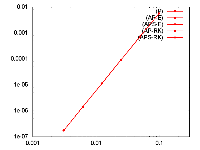
(a) $\varepsilon=1$

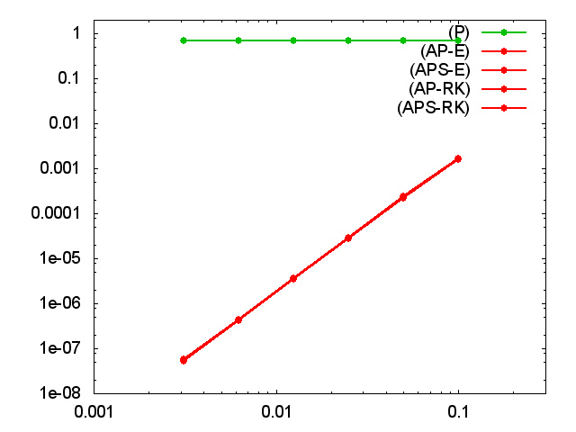
(b) $\varepsilon=10^{-20}$

Figure 1: Relative $L^{2}$-errors between the exact solution $u^{\varepsilon}$ and the computed solution for the standard scheme (P), the Euler-AP method ($E_{AP}$) the stabilized Euler-APS method ($E_{APS}$), the DIRK-AP scheme ($RK_{AP}$) and the stabilized DIRK-APS scheme ($RK_{APS}$) as a function of $h$, for $\varepsilon=1$ resp. $\varepsilon=10^{-20}$ and the time step $\tau=10^{-6}$. Observe that for $\varepsilon=1$ all schemes give the same precision, for $\varepsilon=10^{-20}$ the standard scheme does not work while all AP schemes give comparable accuracy.

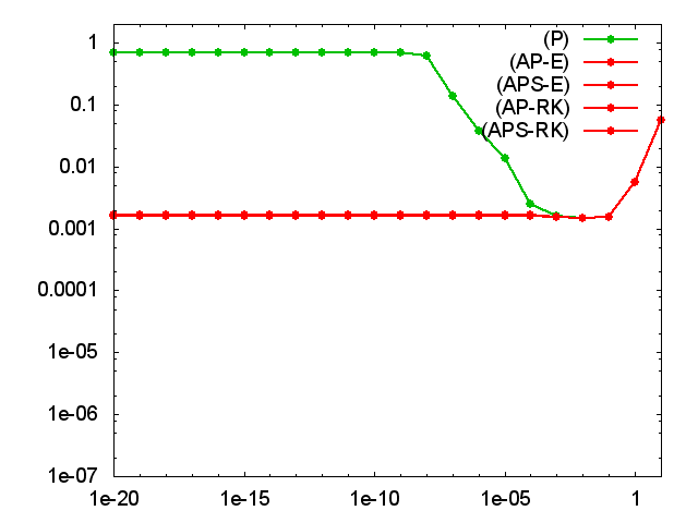
(a) $h=0.1$

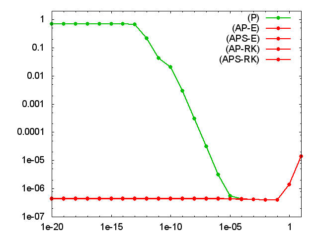
(b) $h=0.00625$

Figure 2: Relative $L^{2}$-errors between the exact solution $u^{\varepsilon}$ and the computed solution for the standard scheme (P), the Euler-AP method ($E_{AP}$) the stabilized Euler-APS method ($E_{APS}$), the DIRK-AP scheme ($RK_{AP}$) and the stabilized DIRK-APS scheme ($RK_{APS}$) as a function of $\varepsilon$, for $h=0.1$ resp. $h=0.00625$ and the time step $\tau=10^{-6}$. Observe that the standard scheme is accurate only for small values of anisotropy (large $\varepsilon$) while all AP schemes give comparable accuracy in the whole range of $\varepsilon$.

Next, the time convergence of the methods is tested. In this case the mesh size is chosen in such a way that the space discretization does not influence the numerical precision (at least for large time steps). We perform simulations for different time steps and for a fixed final time ($t=0.1$). The results are presented in Table 2 and Figure 3. The time discretization convergence order is confirmed. The $(RK_{AP})$ and $(RK_{APS})$ schemes are, as expected, of second order in time as long as the error due to the space discretization is smaller than the error induced by the time discretization. The $(E_{AP})$ and $(E_{APS})$ schemes are of first order for all values of the anisotropy parameter and the standard (P)-scheme works well and is of first order where the anistropy is weak ($\varepsilon$ close to one). Note that the stabilization procedure does not influence the accuracy of the solution if the time discretization error is bigger than the space discretization error. One can also observe that reasonably accurate results are obtained even with relatively large time steps, especially for the Runge-Kutta schemes. This property would allow orders of magnitude gains in integration time for a given physics application with respect to non-AP schemes.

$\tau$	$L^{2}$-error  $\varepsilon=1$
	P	$E_{AP}$	$E_{APS}$	$RK_{AP}$	$RK_{APS}$
0.1	$1.32\times 10^{-3}$	$1.32\times 10^{-3}$	$1.32\times 10^{-3}$	$8.4\times 10^{-5}$	$8.4\times 10^{-5}$
0.05	$7.2\times 10^{-4}$	$7.2\times 10^{-4}$	$7.2\times 10^{-4}$	$2.43\times 10^{-5}$	$2.43\times 10^{-5}$
0.025	$3.55\times 10^{-4}$	$3.55\times 10^{-4}$	$3.55\times 10^{-4}$	$6.2\times 10^{-6}$	$6.2\times 10^{-6}$
0.0125	$1.75\times 10^{-4}$	$1.75\times 10^{-4}$	$1.75\times 10^{-4}$	$1.59\times 10^{-6}$	$1.59\times 10^{-6}$
0.00625	$8.8\times 10^{-5}$	$8.8\times 10^{-5}$	$8.8\times 10^{-5}$	$4.8\times 10^{-7}$	$4.8\times 10^{-7}$
0.003125	$4.4\times 10^{-3}$	$4.4\times 10^{-3}$	$4.4\times 10^{-3}$	$2.82\times 10^{-5}$	$2.82\times 10^{-5}$
0.0015625	$2.20\times 10^{-5}$	$2.20\times 10^{-5}$	$2.20\times 10^{-5}$	$2.64\times 10^{-7}$	$2.64\times 10^{-7}$

$\tau$	$L^{2}$-error  $\varepsilon=10^{-20}$
	P	$E_{AP}$	$E_{APS}$	$RK_{AP}$	$RK_{APS}$
0.1	$2.28\times 10^{-1}$	$1.14\times 10^{-3}$	$1.14\times 10^{-3}$	$7.4\times 10^{-5}$	$7.4\times 10^{-5}$
0.05	$2.53\times 10^{-1}$	$6.2\times 10^{-4}$	$6.2\times 10^{-4}$	$2.10\times 10^{-5}$	$2.10\times 10^{-5}$
0.025	$2.53\times 10^{-1}$	$3.07\times 10^{-4}$	$3.07\times 10^{-4}$	$5.3\times 10^{-6}$	$5.3\times 10^{-6}$
0.0125	$2.50\times 10^{-1}$	$1.51\times 10^{-4}$	$1.51\times 10^{-4}$	$1.33\times 10^{-6}$	$1.33\times 10^{-6}$
0.00625	$2.51\times 10^{-1}$	$7.6\times 10^{-5}$	$7.6\times 10^{-5}$	$3.44\times 10^{-7}$	$3.44\times 10^{-7}$
0.003125	$2.53\times 10^{-1}$	$3.81\times 10^{-5}$	$3.81\times 10^{-5}$	$1.18\times 10^{-7}$	$1.18\times 10^{-7}$
0.0015625	$2.53\times 10^{-1}$	$1.90\times 10^{-5}$	$1.90\times 10^{-5}$	$8.3\times 10^{-8}$	$8.3\times 10^{-8}$

Table 2: The absolute error of $u$ in the $L^{2}$-norm for different time step using the singular perturbation scheme (P) and two proposed AP-schemes for mesh size $200\times 200$ at time $t=0.1$.

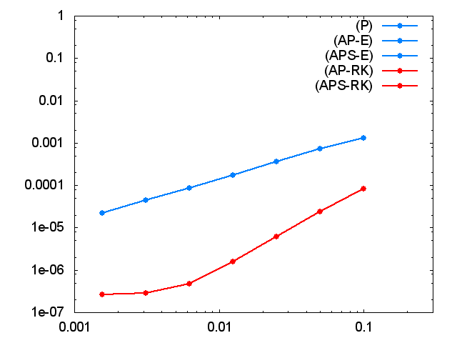
(a) $\varepsilon=1$

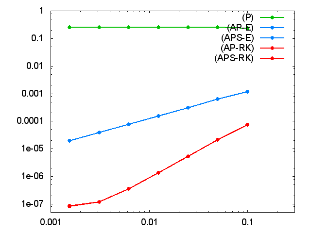
(b) $\varepsilon=10^{-20}$

Figure 3: Relative $L^{2}$-errors between the exact solution $u^{\varepsilon}$ and the computed solution with the standard scheme (P), the Euler-AP method ($E_{AP}$) the stabilized Euler-APS method ($E_{APS}$), the DIRK-AP scheme ($RK_{AP}$) and the stabilized DIRK-APS scheme ($RK_{APS}$) as a function of $\tau$, and for $\varepsilon=1$ resp. $\varepsilon=10^{-20}$ and a mesh with $200\times 200$ points.

Numerical test have confirmed that all asymptotic preserving schemes are accurate independently of $\varepsilon$. The penalty stabilization procedure can introduce a very small amount of additional error in some configurations, but the order of convergence is conserved. In the following experiments, the stabilized schemes are tested on the case of $b$ containing closed field lines.

4.3 Temperature balance in the presence of magnetic islands

In this section we perform a numerical experiment related to the tokamak plasma. This numerical test case fully demonstrates the novelty of the proposed stabilized AP scheme as it can applied in more general settings as the previous ones [5, 11]. The results of this section show that it is capable of simulating the heat transfer in the presence of the closed field lines in the computational domain.

We consider a square computational domain $\Omega=[-0.5,0.5]\times[-0.5,0.5]$ and a field $b$ with a perturbation consisting of a region with closed lines. This so called magnetic island is initially localized in the center of the domain and moving with the velocity $\omega$. The field is given by

$$b=\frac{B}{|B|}\,,\quad B=\left(\begin{array}[]{c}-A2\pi\sin(2\pi(y-\omega t))\\ \pi\sin(\pi x)\end{array}\right),$$ (34)

where $A$ is a perturbation parameter related to the island’s width $w=4A^{1/2}/\pi$. This is the largest distance between the two branches of the separatrix, the line that divides the domain into regions of open and closed field lines. The two branches meet at the X-point, the saddle point of the vector potential. The island center, an extremum of the vector potential, is referred to as the O-point. If $A=0$ the obtained field is aligned with the $Y$ axis and points upwards (downwards) for $x>0$ ($x<0$). For $A>0$ the magnetic island consisting of closed field lines appears in the region around $x=0$.

Referring to the theory of magnetic islands, this magnetic field geometry approximates a saturated tearing mode in the so called constant-$\psi$ regime (whence the parameter $A$ is a constant). The frequency describes the rotation of an island as observed in experiments and numerical simulations.

This frequency is typically of the order of the diamagnetic frequency, which is smaller than the Alfven frequency (the propagation rate of an Alfven wave), but larger than the transport rate across a typical island. It is thus interesting to study heat transport in an island that rotates sufficiently fast.

For a static island or one rotating sufficiently slowly, we expect the fast transport along the field lines to flatten the temperature profile in the island region.

We choose to impose periodic boundary conditions on $\{(x,y)\in\partial\Omega\ |y=-0.5\}\cup\{(x,y)\in\partial\Omega\ |y=0.5\}$ so the domain is topologically equivalent to the surface of a torus. We supply the computational domain with two sets of conditions on remaining boundaries:

1. Dirichlet boundary conditions $\Gamma_{D}=\{(x,y)\in\partial\Omega\ |x=-0.5\}\cup\{(x,y)\in\partial\Omega\ |x=0.5\}$ with

   $$g_{D}(t,\cdot)=\left\{\begin{array}[]{ll}1&\text{ for }x=-0.5\\ 0&\text{ for }x=0.5\end{array}\right.,$$ (36)

   where temperature is exchanged with the exterior only by a $\Gamma_{D}$ boundary.

2. Neumann and Dirichlet boundary conditions: $\Gamma_{N}=\{(x,y)\in\partial\Omega\ |x=-0.5\}$ and $\Gamma_{D}=\{(x,y)\in\partial\Omega\ |x=0.5\}$ with

   $${\quad\quad}g_{N}(t,\cdot)=1,{\quad\quad}{\quad\quad}g_{D}(t,\cdot)=0,$$ (37)

   which corresponds to the constant heating of the left side of the computational domain.

In the case of the boundary conditions of the first type we expect that the presence of the island should increase the gradient of the temperature outside the island region and keep the temperature constant inside the island in such way that the total energy of the system remains unchanged. If the boundary conditions are of the second type, i.e. in the heating case, the gradient of the temperature in the non-island region should remain constant leading thus to a loss of the total energy of the system.

We perform simulations with fixed $\varepsilon=10^{-10}$ and $A=0.01$, giving an island of a width $w=0.4/\pi\approx 13\%$. The magnetic field lines are shown on Figure 4. The initial conditions for both boundary types are the same and correspond to the stationary solution with no island present. That is to say, $u^{0}(x,y)=-x+\frac{1}{2}$. We perform our simulations on a fixed grid of $200\times 200$ points for 100 time steps $\tau=2.5\times 10^{-3}$ until the final time $0.25$ is reached. We compare results for a stationary island ($\omega=0$) and a moving island ($\omega=10$) with no island case. We are interested in the temperature profile along the $X$ axis as well as in the total energy of the system, i.e. integral of the temperature in the computational domain.

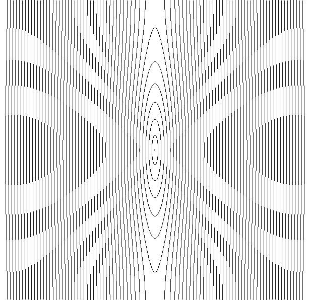
Figure 4: Magnetic island for $A=0.01$

4.3.1 Dirichlet boundary condition on the left edge (36)

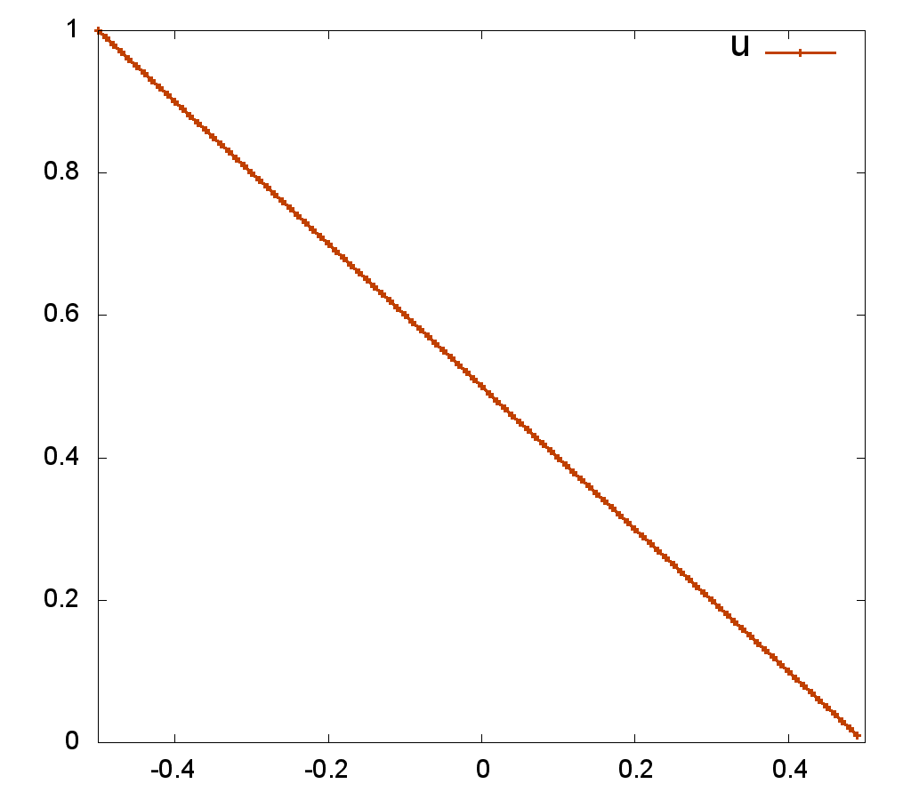
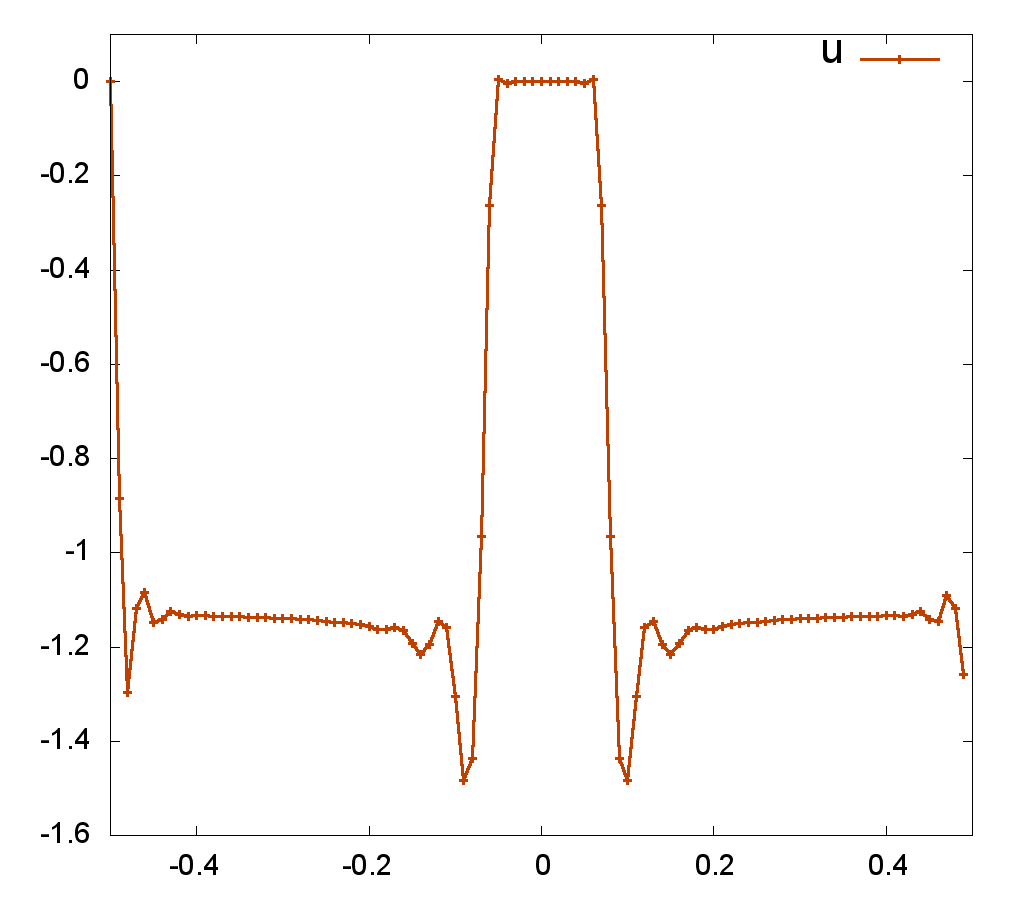
Figure 5: Temperature profiles (top row) and temperature gradients (bottom row) along the $X$ axis for non perturbed field ($A=0$) on the left and a stationary island ($A=0.01$) present in the center of the domain on the right for the Dirichlet BC.

Numerical results confirm our expectations. The total energy remains constant in the system. Integral of the temperature in the computational domain equals to $1/2$ in all three cases: for a stationary island, moving island and non perturbed system. The temperature is constant in the island region leading to a stronger gradient outside the perturbation. Temperature profiles along the $X$ axis are shown on Figures 5 and 6. In the case of a moving island the width of a constant temperature region in the temperature profile along the $X$ axis is oscillating in time as the island moves in the domain. It is interesting to note that even at the time when there are no closed field lines across the $X$ axis the flat region can be observed. In fact, the $x$ component of temperature gradient is negative but close to zero in this region. Remark also that the temperature gradient increases, approaching zero, near the island at its largest width, i.e. across the O-point. One refers to this effect as ”profile flattening”.

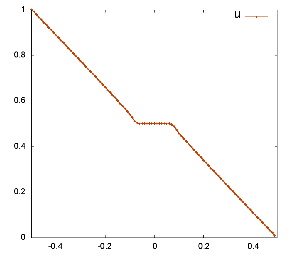
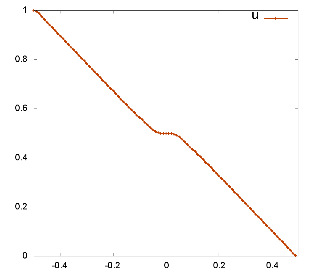
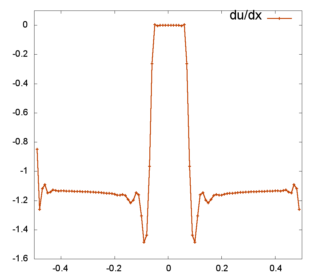
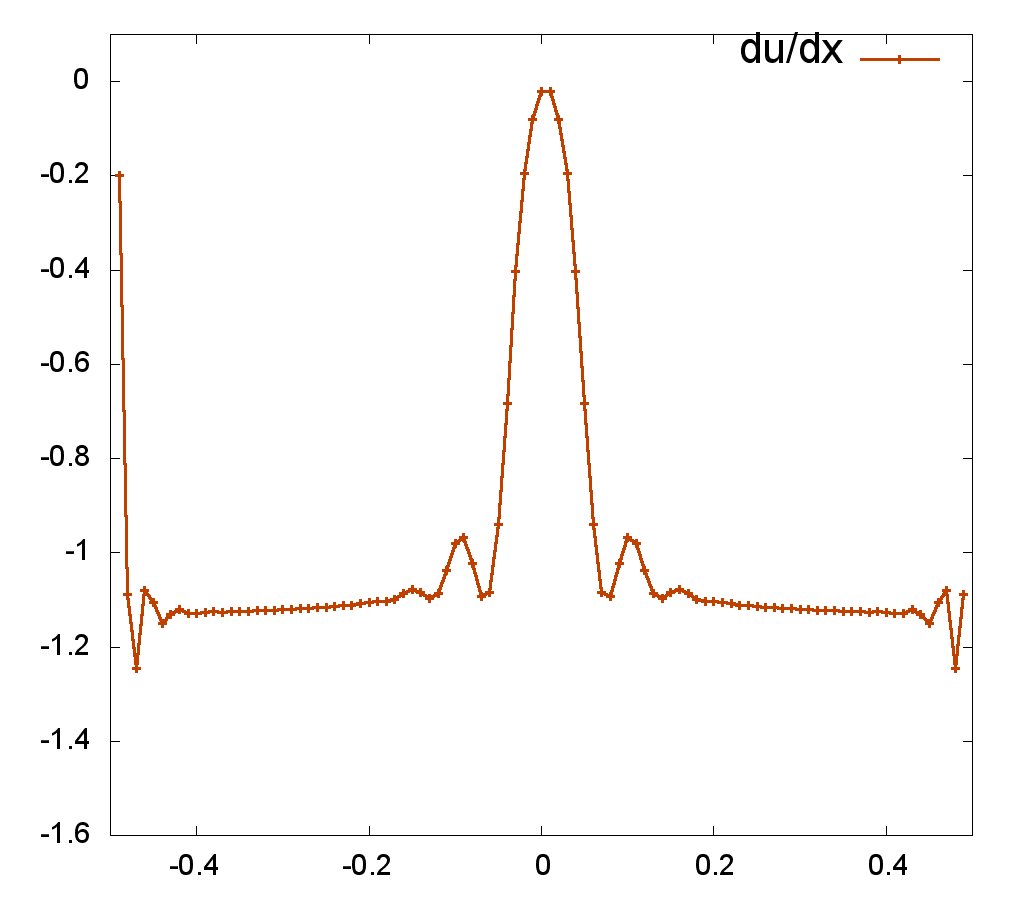
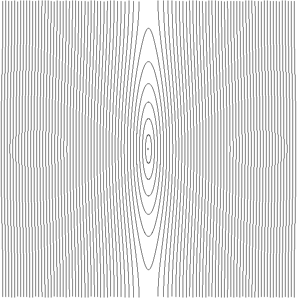
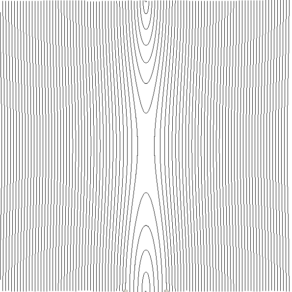
$t=0.1$	$t=0.15$

Figure 6: Temperature profiles along the $X$ axis for a moving island ($A=0.01$, $\omega=10$) in the first row, $x$ component of temperature gradient in the second row and a corresponding anisotropy field in the last row for different time steps for the Dirichlet BC.

4.3.2 Neumann boundary condition on the left edge (37)

In the case of Neumann boundary condition imposed on the left boundary of the domain the results again are consistent with our expectation. The presence of the island reduces the total energy. Integral of the temperature drops from $0.5$ to $0.44$ and the maximal temperature from $1$ to $0.89$ for both stationary and moving island. Temperature profiles along the $X$ axis are shown on Figures 7 and 8. The results are very similar to those in the previous test case. The difference is in the maximal temperature and in the temperature gradient in the $X$ direction, which is now close to one in the regions far from the island. This is of course what is expected and consistent with the heating imposed on the left boundary by the means of Neumann boundary condition.

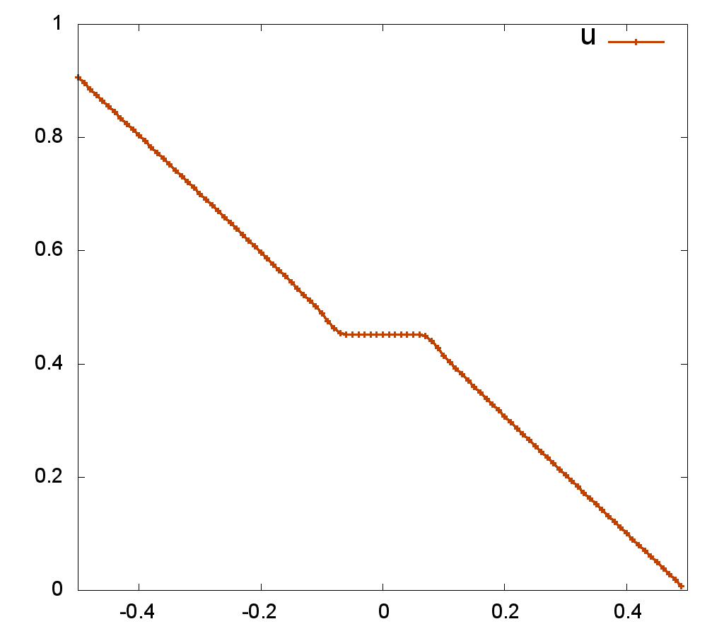
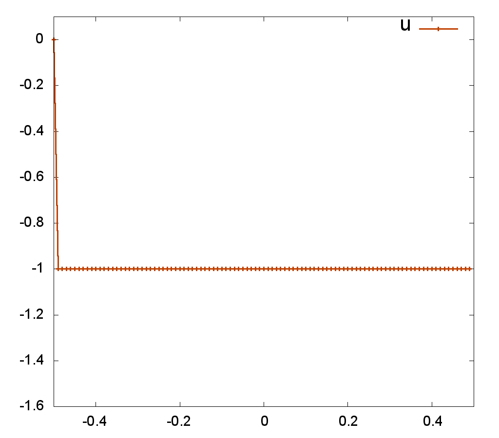
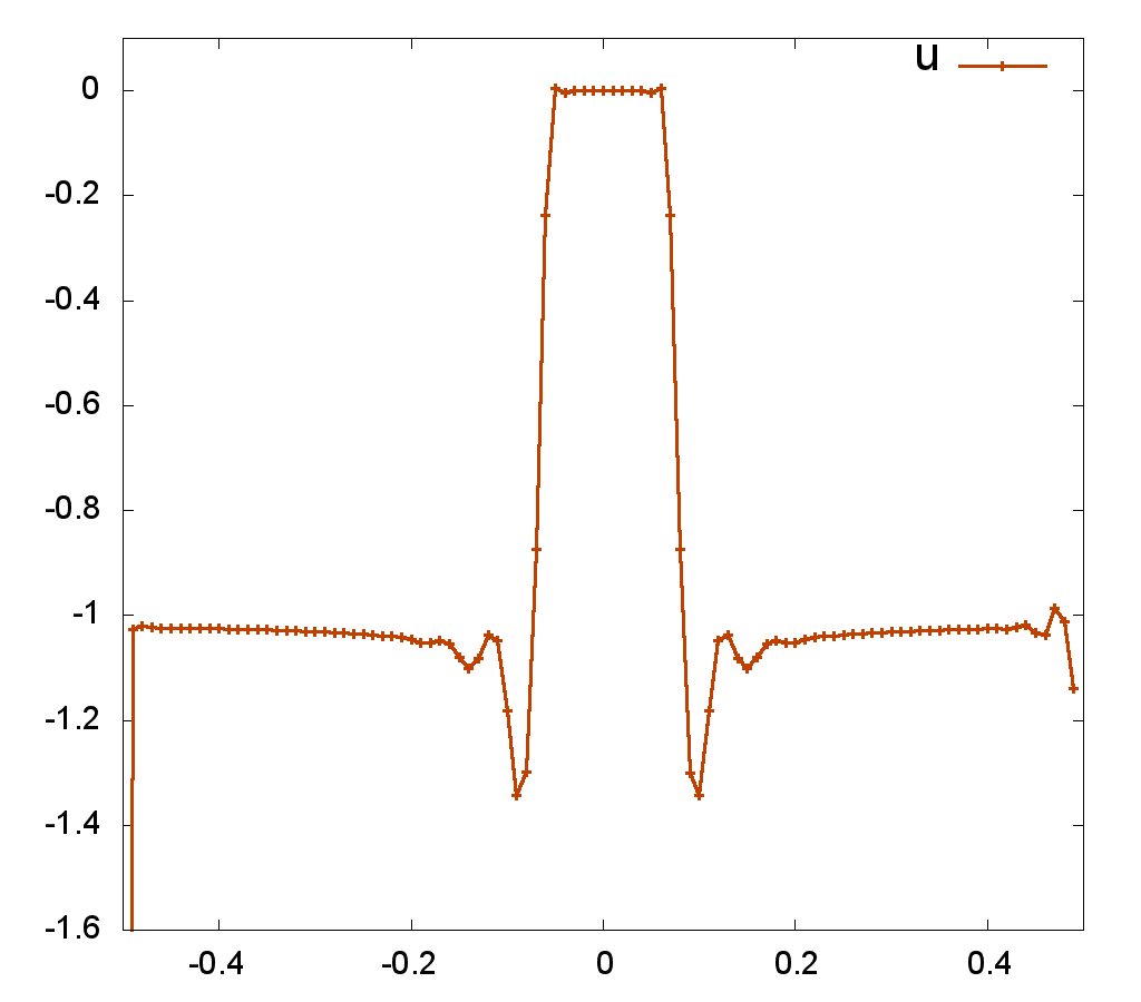
Figure 7: Temperature profiles (top row) and temperature gradients (bottom row) along the $X$ axis for non perturbed field ($A=0$) on the left and a stationary island ($A=0.01$) present in the center of the domain on the right for the Neumann BC.

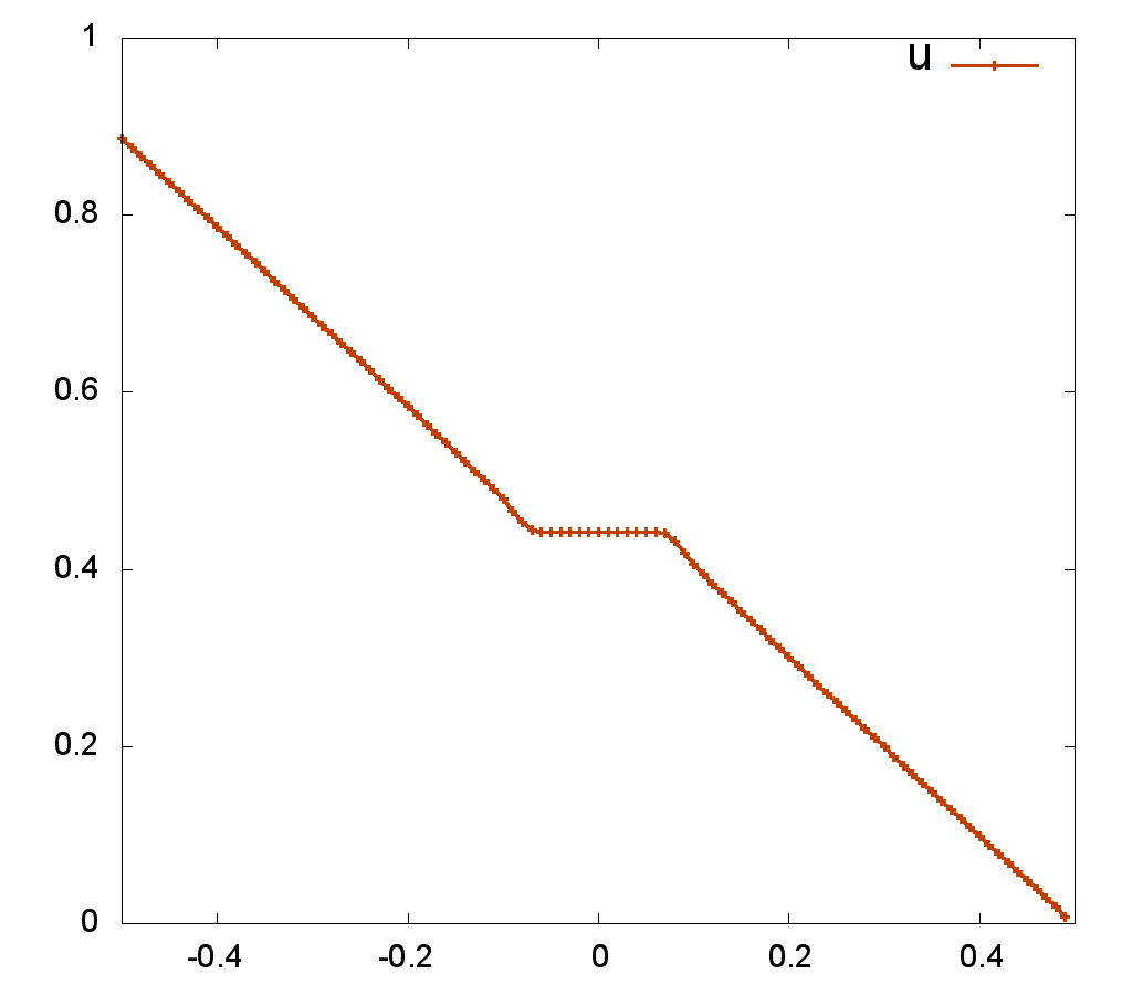
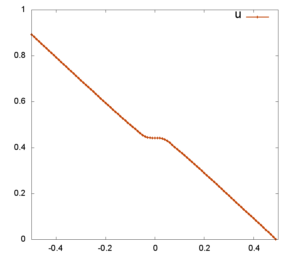
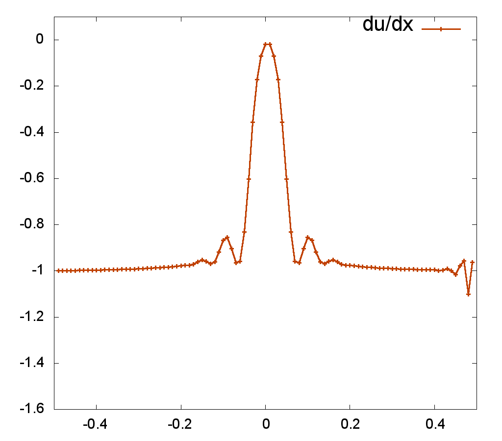
$t=0.1$	$t=0.15$

Figure 8: Temperature profiles along the $X$ axis for a moving island ($A=0.01$, $\omega=10$) in the first row and the $x$ component of temperature gradient in the second row for different time steps for the Neumann BC.

4.3.3 Fast rotating magnetic island with Dirichlet boundary condition on the left edge (36)

In the last experiment we study the effect of the islands rotation speed on the temperature profile. We expect to see a different temperature profile when the rotation is faster than the transport rate in the parallel direction. To achieve this numerically we decrease the island width such that $A=0.000625$, augment the mesh size to $500\times 500$, decrease the size of the computational domain $\Omega=[-0.125,0.125]\times[-0.5,0.5]$ and put $\varepsilon=10^{-3}$. We also increase the time resolution and put $\tau=0.25\times 10^{-6}$ and vary the rotation speed from $10^{3}$ to $10^{6}$. Then we compare temperature profiles after 10000 time steps.

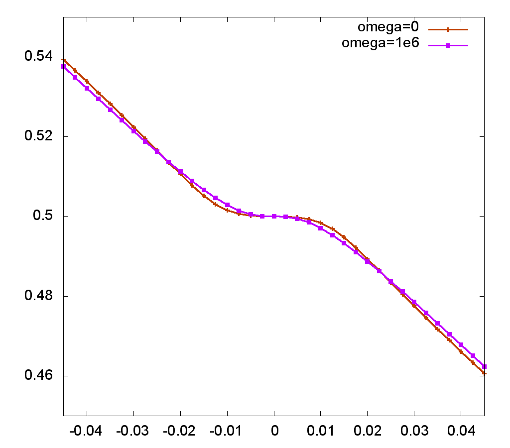
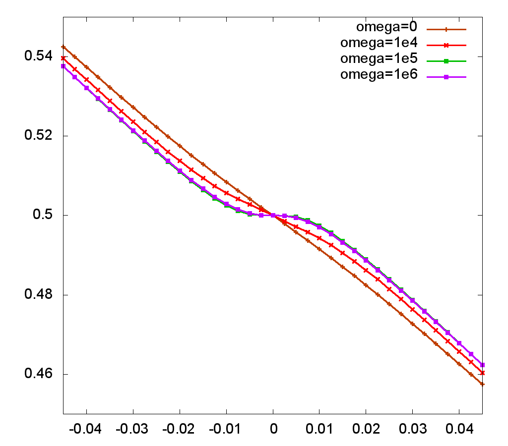
Figure 9: Comparison between temperature profiles along the $X$ axis for the stationary and rotating islands. The profile across the island center ($Y=Y_{C}$) on the left and away from the center ($Y=Y_{C}\pm 0.5$) on the right.

For the smallest rotation velocity ($\omega=10^{3}$) no deviation from the stationary case is observed. For other velocities the temperature profile across the islands center is only slightly affected by the rotation velocity. The most interesting effect of the velocity is visible on the profile taken away from the island. In the stationary case the profile is a straight line with a constant gradient. If the rotation velocity is big enough, the profile begins to slightly flatten near the center ($X=0$) for $\omega=10^{4}$ and finally looks exactly the same as for the islands center ($\omega=10^{5}$ and $\omega=10^{6}$). In fact, for a sufficiently big rotation speed the temperature profile becomes homogeneous, i.e. independent of $Y$. A zoom of temperature profiles at the islands center ($Y=Y_{C}$) and at the most distant from the islands center $Y$ ($Y=Y_{C}+0.5$ if $Y_{C}<0$ and $Y=Y_{C}-0.5$ otherwise) is presented on Figure 9.

5 Conclusion

The here presented Asymptotic-Preserving scheme proves to be an efficient, general and easy to implement numerical method for solving strongly anisotropic parabolic problems. As numerical experiments show, the second order two stage Runge-Kutta scheme is of particular interest as it produces accurate results for relatively large time steps allowing to substantially reduce the computational time. The herein introduced stabilization term is an important improvement to the previously proposed Asymptotic Preserving schemes. The not so rare in real applications anisotropy topologies can be successfully addressed with this new method. Finally, the case of magnetic islands studied in the last section brings new and interesting results showing the homogenization of the temperature profile for fast rotating islands.

References

- [1] M. Beer, S. Cowley, and G. Hammett. Field-aligned coordinates for nonlinear simulations of tokamak turbulence. Physics of Plasmas, 2(7):2687, 1995.
- [2] B. Berkowitz. Characterizing flow and transport in fractured geological media: A review. Advances in Water Resources, 25(8-12):861–884, 2002.
- [3] A. H. Boozer. Establishment of magnetic coordinates for a given magnetic field. Physics of Fluids, 25(3):520–521, 1982.
- [4] P. Degond, F. Deluzet, A. Lozinski, J. Narski, and C. Negulescu. Duality-based asymptotic-preserving method for highly anisotropic diffusion equations. Commun. Math. Sci., 10(1):1–31, 2012.
- [5] P. Degond, A. Lozinski, J. Narski, and C. Negulescu. An asymptotic-preserving method for highly anisotropic elliptic equations based on a micro-macro decomposition. Journal of Computational Physics, 231(7):2724–2740, 2012.
- [6] M. W. Gee, J. J. Hu, and R. S. Tuminaro. A new smoothed aggregation multigrid method for anisotropic problems. Numer. Linear Algebra Appl., 16(1):19–37, 2009.
- [7] S. Günter, K. Lackner, and C. Tichmann. Finite element and higher order difference formulations for modelling heat transport in magnetised plasmas. Journal of Computational Physics, 226(2):2306–2316, 2007.
- [8] S. G nter, Q. Yu, J. Kr ger, and K. Lackner. Modelling of heat transport in magnetised plasmas using non-aligned coordinates. Journal of Computational Physics, 209(1):354 – 370, 2005.
- [9] S. Hamada. Hydromagnetic equilibria and their proper coordinates. Nucl. Fusion, 2:23–37, 1962.
- [10] S. Jin. Efficient asymptotic-preserving (AP) schemes for some multiscale kinetic equations. SIAM J. Sci. Comput., 21(2):441–454, 1999.
- [11] A. Lozinski, J. Narski, and C. Negulescu. Highly anisotropic temperature balance equation and its asymptotic-preserving resolution. arXiv:1203.6739, 2012.
- [12] T. Manku and A. Nathan. Electrical properties of silicon under nonuniform stress. Journal of Applied Physics, 74(3):1832–1837, 1993.
- [13] A. Mentrelli and C. Negulescu. Asymptotic preserving scheme for highly anisotropic, nonlinear diffusion equations. application: Sol plasmas. submitted to JCP, 2012.
- [14] J. Narski. Anisotropic finite elements with high aspect ratio for an asymptotic preserving method for highly anisotropic elliptic equations. submitted, arXiv preprint arXiv:1302.4269, 2013.
- [15] M. Ottaviani. An alternative approach to field-aligned coordinates for plasma turbulence simulations, 2011.
- [16] P. Perona and J. Malik. Scale-space and edge detection using anisotropic diffusion. Pattern Analysis and Machine Intelligence, IEEE Transactions on, 12(7):629–639, 1990.
- [17] P. Sharma and G. W. Hammett. Preserving monotonicity in anisotropic diffusion. J. Comput. Phys., 227:123–142, November 2007.
- [18] P. Sharma and G. W. Hammett. A fast semi-implicit method for anisotropic diffusion. Journal of Computational Physics, 230(12):4899–4909, 2011.
- [19] J. Weickert. Anisotropic diffusion in image processing. European Consortium for Mathematics in Industry. B. G. Teubner, Stuttgart, 1998.