A generalized Beraha conjecture for non-planar graphs

Abstract

We study the partition function $Z_{G(nk,k)}(Q,v)$ of the $Q$–state Potts model on the family of (non-planar) generalized Petersen graphs $G(nk,k)$. We study its zeros in the plane $(Q,v)$ for $1\leq k\leq 7$. We also consider two specializations of $Z_{G(nk,k)}$, namely the chromatic polynomial $P_{G(nk,k)}(Q)$ (corresponding to $v=-1$), and the flow polynomial $\Phi_{G(nk,k)}(Q)$ (corresponding to $v=-Q$). In these two cases, we study their zeros in the complex $Q$–plane for $1\leq k\leq 7$. We pay special attention to the accumulation loci of the corresponding zeros when $n\to\infty$. We observe that the Berker–Kadanoff phase that is present in two–dimensional Potts models, also exists for non-planar recursive graphs. Their qualitative features are the same; but the main difference is that the role played by the Beraha numbers for planar graphs is now played by the non-negative integers for non-planar graphs. At these integer values of $Q$, there are massive eigenvalue cancellations, in the same way as the eigenvalue cancellations that happen at the Beraha numbers for planar graphs.

Key Words: Potts model; non-planar graphs; Beraha conjecture; generalized Petersen graphs; transfer matrix; Berker-Kadanoff phase.

1 Introduction

The two–dimensional (2D) $Q$–state Potts model [41, 58] is one of the most studied models in Statistical Mechanics. Despite many efforts over more than 60 years, its exact free energy and phase diagram are still unknown. The ferromagnetic regime of the Potts model is the best understood case: exact (albeit not always rigorous) results have been obtained for the ferromagnetic-paramagnetic phase transition temperature $T_{\rm c}(Q)$ for several regular lattices, the order of the transition (continuous for $0\leq Q\leq 4$, and first order for $Q>4$), the phase diagram, and the characterization in terms of conformal field theory (CFT) of the corresponding universality classes. (See e.g., Ref. [3].)

The antiferromagnetic (AF) regime is less understood. This is partly because, in contrast with the ferromagnetic regime, universality cannot be expected to hold in general. Investigations must therefore proceed on a case-by-case basis. For instance, the free energy is known exactly along some curves of the phase diagram $(Q,T)$ (where $T$ is the temperature), for certain regular 2D lattices [4, 3]. One of these curves belongs to the ferromagnetic regime, and it can be identified with the ferromagnetic-paramagnetic phase-transition curve. It might be tempting to infer the very existence of a phase transition from this (partial) solubility of the model along that curve. One well-known example of the invalidity of such an inference is provided by the zero-temperature limit of the triangular-lattice $Q$–state Potts antiferromagnet [5, 6]. Although its free energy is exactly known for all values of $Q\in{\mathbb{R}}$, the system is known to be critical only in the interval $Q\in[0,4]$, and disordered for $Q\in(-\infty,0)\cup(4,\infty)$.

In three dimensions (3D) there are no known exact results for the $Q$–state Potts model. Most numerical results come from series expansions and Monte Carlo simulations: see e.g., Refs. [23, 37, and references therein]. In the ferromagnetic regime, we expect a critical curve, which is second order for $Q=2$, and first-order for $Q=3$. There was an important controversy in the late 80s and early 90s about the precise nature of the $Q=3$ transition because of its relation with QCD: the four-dimensional SU(3) lattice gauge theory should be in the same universality class as the 3D ferromagnetic 3–state Potts model [37].

The $Q$–state Potts model at temperature $T$ can be defined on any (undirected) finite graph $G=(V,E)$ with vertex set $V$ and edge set $E$. On each vertex $i\in V$, we place a spin that can take $Q$ distinct values: $\sigma_{i}\in\{1,2,\ldots,Q\}$. These spins interact through the Hamiltonian [41]

$$\mathcal{H}(\{\sigma\})\;=\;-J\sum_{\langle ij\rangle\in E}\delta_{\sigma_{i}\sigma_{j}}\;,$$ (1.1)

where $\delta_{ij}$ is the usual Kronecker delta, and $J$ is a real coupling constant that is proportional to $1/T$. The partition function is defined as usual as:

$$Z_{G}(Q,v)\;=\;\sum\limits_{\{\sigma\}}e^{-{\mathcal{H}}}\,.$$ (1.2)

Notice that initially, $Q$ is a positive integer $Q\geq 2$, and $J$ is a real number. The ferromagnetic (resp. antiferromagnetic) regime corresponds to $J\geq 0$ (resp. $J\leq 0$).

Fortuin and Kasteleyn [22] have shown that the partition function (1.2) can be rewritten as

$$Z_{G}(Q,v)\;=\;\sum\limits_{E^{\prime}\subseteq E}v^{|E^{\prime}|}Q^{k(E^{\prime})}\,,$$ (1.3)

where the sum runs over the $2^{|E|}$ subsets $E^{\prime}\subseteq E$, with $k(E^{\prime})$ being the number of connected components (including isolated vertices) in the spanning subgraph $(V,E^{\prime})$, and $v$ is the temperature-like parameter

$$v\;=\;e^{J}-1\,.$$ (1.4)

We now can promote (1.3) to the definition of the model, which permits us to consider the parameters $Q$ and $v$ as arbitrary complex numbers, because (1.3) is a polynomial in both. The Fortuin–Kasteleyn (FK) representation of the $Q$–state Potts model (1.3) is equivalent to the Tutte polynomial studied by graph theorists [55] after a change of variables. In terms of $v$, the ferromagnetic (resp. antiferromagnetic) regime corresponds to $v\geq 0$ (resp. $-1\leq v\leq 0$). The unphysical regime corresponds to $v<-1$ (i.e., complex $J$), and the behavior of the Potts model in this regime is less well understood than that of the AF regime.

There are several interesting particular cases of $Z_{G}(Q,v)$. One first example is the chromatic polynomial

$$P_{G}(Q)\;=\;Z_{G}(Q,-1)\,,$$ (1.5)

which corresponds to the zero-temperature limit in the AF regime $J\to-\infty$. The restriction of this polynomial to $Q$ a positive integer has indeed an interpretation as a coloring problem [16]: $P_{G}(Q)$ gives the number of proper $Q$-colorings of the graph $G$. A proper $Q$-coloring of a graph $G=(V,E)$ is a coloring of the vertices in $V$ such that for each edge $e=\langle i,j\rangle\in E$ its endpoints $i,j$ are not colored alike.

The second example is the flow polynomial

$$\Phi_{G}(Q)\;=\;(-1)^{|E|}Q^{-|V|}Z_{G}(Q,-Q)\,.$$ (1.6)

Again, the restriction of this polynomial to integer $Q$ has a combinatorial interpretation: it gives the number of nowhere ${\mathbb{Z}}_{Q}$-flows on $G$. If $\Gamma$ is an additive Abelian group of order $Q$, a $\Gamma$-flow on $G$ is a function $\phi\colon E\mapsto\Gamma$, so that each edge $e\in E$ is associated to a variable $\phi(e)$, subject to the constraint that these variables are conserved at each vertex $i\in V$, given an arbitrary orientation of the edges in $E$. A no-where zero $\Gamma$-flow is a $\Gamma$-flow $\phi$ such that $\phi(e)\neq 0$ for all edges $e\in E$ [56, 36, 60]. If $\Gamma$ is a finite Abelian group of order $Q$, then the number of nowhere zero $\Gamma$-flows depends only on $Q$ (not on the specific structure of the group $\Gamma$), and it is in fact the restriction to $Q\in{\mathbb{N}}$ of a polynomial in $Q$ called the flow polynomial $\Phi_{G}(Q)$ [54]. We choose $\Gamma={\mathbb{Z}}_{Q}$ as our group of order $Q$.

These two polynomials are related for planar graphs. This relation is based on the duality transformation for the $Q$-state Potts model on a planar graph $G$ [59]:

$$Z_{G}(Q,v)\;=\;Q^{|V|-|E|-1}\,v^{|E|}\,Z_{G^{*}}(Q,v^{*})\,,$$ (1.7)

where $G^{*}$ is the dual graph of $G$, and $v^{*}$ is the dual of $v$

$$v\,v^{*}\;=\;Q\,.$$ (1.8)

Then for $v=-1$, $v^{*}=-Q$, so that (1.7) reduces to

$$P_{G^{*}}(Q)\;=\;Q\,\Phi_{G}(Q)\,,$$ (1.9)

The duality relation (1.9) can also be understood combinatorially: the flow along an edge $e\in E$ of $G$ determines the color difference between the two faces (vertices of $G^{*}$) that are adjacent to $e$. The conservation of the ${\mathbb{Z}}_{Q}$-flow at each vertex $i\in V$ ensures that the color differences thus defined add up to zero upon encircling $i$. A definite $Q$-coloring of $G^{*}$ is obtained from these color differences upon fixing the color of one reference vertex; this is responsible for the factor of $Q$ appearing in (1.9).

For non-planar graphs there is no known relation whatsoever between $\Phi_{G}(Q)$ and $P_{G^{*}}(Q)$.

The evaluation of $Z_{G}(Q,v)$ for a general graph is a hard problem, viz., at least as demanding as the determination of the chromatic or the flow polynomials. In particular, the determination of the coefficients of the chromatic or flow polynomials of a general graph (including bipartite planar graphs) is #P-hard [38, Proposition 2.1], and the same thus holds in general for the computation of the coefficients of the full partition function $Z_{G}(Q,v)$. For recursive families of graphs, the partition function $Z_{G_{n}}(Q,v)$ of any member of the family $G_{n}$ (composed by $n$ identical layers of size $m$ each) can be computed from a transfer matrix $\mathsf{T}$ and certain boundary condition vectors $\bm{u}$ and $\bm{v}$:

$$Z_{G_{n}}(Q,v)\;=\;\bm{u}(m)^{t}\cdot\mathsf{T}(m)^{n}\cdot\bm{v}(m)\,,$$ (1.10)

where $t$ denotes the transpose. The computation time thus grows as a polynomial in $n$; but it does however still grow exponentially in $m$. Indeed, there are similar formulas for computing $P_{G}$ and $\Phi_{G}$ directly from the corresponding transfer matrices. The partition function (1.10) can be written as a sum over the eigenvalues $\lambda_{j}$ of the transfer matrix $\mathsf{T}$ with appropriate amplitudes $\alpha_{j}$:

$$Z_{G_{n}}(Q,v)\;=\;\sum\limits_{j=1}^{\mathop{\rm dim}\nolimits\mathsf{T}}\alpha_{j}\,\lambda_{j}^{n}\,,$$ (1.11)

where both the amplitudes and eigenvalues are algebraic functions of both $Q$ and $v$.

From (1.10) one can compute the partition function $Z_{G_{n}}$ of the $Q$-state Potts model (or any of its specializations $P_{G_{n}}$ or $\Phi_{G_{n}}$) on any member $G_{n}$ of a recursive family of graphs. In practice, this family of graphs will be a 2D strip graph of some regular lattice of width $m$ and length $n$ with some boundary conditions. In this case, we will simplify the notation by writing $Z_{m_{\alpha}\times n_{\beta}}$, where the subscripts $\alpha,\beta=\text{F,P}$ denote free and periodic boundary conditions in the respective lattice directions. For 3D “slab” graphs, we use $Z_{m_{\alpha}\times p_{\beta}\times n_{\gamma}}$ for the partition function of a slab of section $m\times p$ and thickness $n$. As the partition function is a polynomial in $Q$ and $v$, we can study its roots, e.g., by fixing $Q$ (resp. $v$) to a physical value and then obtaining the roots of the resulting one-variable polynomial in the complex $v$-plane (resp. $Q$-plane). This programme has been done for 2D strip graphs of the square and triangular lattices with free and cylindrical boundary conditions [18, 17]. Indeed, there are several ways to study the zeros of $Z_{G_{n}}$: for instance, considering the plane $(Q,v)$ where both variables take real values. This approach will produce the “phase diagram” of the model for finite transverse size.

The above study is hard to carry out in practice. In fact, most studies are concerned with the zeros in the complex $Q$-plane of the chromatic polynomial $P_{G}$ (or chromatic zeros of $G$). In a series of papers [46, 27, 31, 28, 29, 47, and references therein], we have studied 2D strip graphs of the square and triangular lattices with free, cylindrical, cyclic, and toroidal boundary conditions. For 3D lattices, the authors of Ref. [45] computed the chromatic roots of “slabs” with some small transverse sections (with free and periodic boundary conditions) and several values of the longitudinal size $n$ (with free boundary conditions). Finally, the roots of the flow polynomial (or flow roots) have been studied for some 2D strip graphs and boundary conditions in Ref. [20].

From these zeros it is very hard to obtain infinite-volume quantities ($m,n\to\infty$), as they have strong finite–size–scaling (FSS) corrections. Moreover, one must face the well-known difficulty that the limits $\lim_{m=n\to\infty}$ (Fisher limit) and $\lim_{m\to\infty}\lim_{n\to\infty}$ (van Hove limit) may give different results in some parts of the parameter space. In this paper we consider the latter limit, which has two major advantages: 1) the first limit, $\lim_{n\to\infty}$, is convenient (and accessible in polynomial time) within the transfer matrix approach, and 2) the resulting FSS dependence in the second limit, $\lim_{m\to\infty}$, is much weaker than when considering the $m$ and $n$ limits simultaneously. In other words, we first compute, for fixed (and small) values of $m$, accumulation sets of partition function zeros in the infinite-length limit $n\to\infty$, and study the infinite-width limit $m\to\infty$ subsequently.

According to the Beraha–Kahane–Weiss (BKW) theorem [11, 12, 10, 13, 53], these zeros accumulate along certain limiting curves $\mathcal{B}_{m}$ (when the two eigenvalues that are largest in modulus become equimodular), and around isolated limiting points (when there is a unique dominant eigenvalue and its amplitude vanishes). By computing the eigenvalues $\lambda_{j}$ and amplitudes $\alpha_{j}$ of the transfer matrix $\mathsf{T}$ (1.11), we are able to obtain the exact values of the relevant physical quantities in the limit $n\to\infty$. Their FSS corrections are found to be smaller than when both $m$ and $n$ are finite. The extrapolation to the true infinite-volume limit $m\to\infty$, using standard FSS techniques, therefore becomes more precise by employing this order of limits.

When looking at the real chromatic zeros for 2D strip graphs of the square and triangular lattices with free, cylindrical and cyclic boundary conditions [46, 27, 31, 28, 47, and references therein], we observe (as many authors in the literature did in the past!) that there exist real accumulation points of these real chromatic roots. This observation dates back to Beraha [9] who made a conjecture about the possible values of $Q$ that can be accumulation points for real chromatic roots. As explained by Saleur [49] there are two statements of the Beraha conjecture that do not seem to be fully equivalent: The first one is contained in Beraha’s PhD Thesis [9] (the statement is taken from Ref. [11]):

Conjecture 1.1 (Beraha v1)

Among the limits of all (not necessarily recursive) families of chromatic polynomials are found the numbers of the form:

$$B_{n}\;=\;2+2\cos\frac{2\pi}{n}\;=\;4\cos^{2}\frac{\pi}{n}\,,$$ (1.12)

for any positive integer $n$. Notice that $B_{1}=\lim_{n\to\infty}B_{n}=4$.

This conjecture has a slightly different form in Baxter’s book [3] (the statement is taken from Ref. [6]):

Conjecture 1.2 (Beraha v2)

Some of the real zeros of chromatic polynomials of planar graphs should, in the limit of the graph becoming large, occur at points in the sequence $B_{n}$ (1.12) with integer $n\geq 2$.

Finally, Jackson [25] states the Beraha conjecture in another slightly different way:

Conjecture 1.3 (Beraha v3)

There exists a plane triangulation with a real chromatic root in $(B_{n}-\epsilon,B_{n}+\epsilon)$ for all $n\geq 2$ and all $\epsilon>0$.

Remark. In the context outlined above, our understanding is that the Beraha conjecture is a statement about the accumulation points of chromatic roots in the infinite-size limit of planar regular graphs. Conjecture 1.2 claims that generically the Beraha numbers are limiting points for the chromatic zeros of families of planar graphs. It is clear that integer Beraha numbers $B_{2},B_{3},B_{4},B_{6}$ can actually be chromatic zeros of planar graphs (e.g., $K_{4}$ has all these numbers as chromatic roots: $P_{K_{4}}(Q)=Q(Q-1)(Q-2)(Q-3)$). However, non-integer Beraha numbers (except perhaps $B_{10}$) cannot be chromatic zeros of any planar graph [46, Corollary 2.4]. Furthermore, $B_{10}$ is not a chromatic zero of any plane near-triangulation [46, Proposition 2.3(c)], nor of any plane triangulation.

Let us now consider a strip graph of a (not necessarily planar) regular lattice with periodic boundary conditions along the longitudinal direction. To treat this case within the transfer matrix formalism, we have to keep track of the bottom- and top-row connectivities. As explained in detail in Refs. [28, 29, 30], the transfer matrix only acts on the top-row connectivity, so the full transfer matrix has a block-diagonal form, each block corresponding to a different bottom-row connectivity. Indeed, there are blocks of the top-row state connected to blocks of the bottom-row state; each of these structures will be called a link (or bridge). As the transfer matrix cannot increase the number of links of a given connectivity state, if we order the state appropriately, the transfer matrix takes an upper-triangular form. Therefore, the eigenvalues can be obtained from those diagonal blocks corresponding to a given number $\ell$ of links. The corresponding amplitudes $\alpha_{\ell}$ are non-trivial and can be inferred either from a combinatorial reasoning applied to the upper-triangular decomposition of the transfer matrix [19, 43, 44], from quantum field theory [50, 42], or from representation theoretical considerations [24]. We now have three cases:

1. The strip is planar with free boundary conditions along the transverse direction. This is the geometry of an annulus. In this case, the links cannot interchange their positions, so the group acting on them is the trivial group $E$ consisting only of the identity. The transfer matrix commutes with the generators of the quantum algebra $U_{q}sl(2)$, with $\sqrt{Q}=q+q^{-1}$. In this case the amplitudes $\alpha_{\ell}$ are given by Chebyshev polynomials of the second kind [40, 50, 19]. The numerical evidence [28] shows that there are accumulation points at the Beraha numbers (1.12). This is compatible with the CFT predictions of the pattern of eigenvalue dominance [50].

2. The strip is planar, but periodic boundary conditions are imposed along the transverse direction. The resulting geometry is that of the torus, which is obviously non-planar. In this case, the links can be cyclically interchanged across the strip. Therefore, the group acting in this situation is the cyclic group $C_{\ell}$. The representation theory of this group leads to very different expressions for the amplitudes [44, Equations (1.2)/(1.3)] (see also [42]) involving number theoretical functions. The fact that the $\ell$ links can now wind around the periodic transverse direction with some momentum $p$ implies that the amplitudes $\alpha_{\ell,p}$ depend on both parameters. In this case the numerical evidence [29], and CFT arguments for the pattern of eigenvalue dominance, shows that there are accumulation points of real zeros at $Q=0,1,2,3,4$.

3. The strip graph itself is non-planar. In this case the links can be interchanged in any way, so the group describing this situation is the full symmetric group $S_{\ell}$. The amplitudes $\alpha_{\ell,\lambda}$ obtained from the representation theory of this group are certain polynomials that depend on $\ell$ and on the irreducible representation $\lambda$ of $S_{\ell}$ [24]. The best numerical evidence comes from the study of the flow polynomial of the generalized Petersen graphs [30]. In this case there are accumulation points of real roots at non-negative integer values of $Q=0,1,2,\ldots$. The present paper extends this evidence to higher values of $Q$, and to the Potts model partition function in general.

Remark. Obvious a planar strip graph is a special case on a non-planar one; yet the results (3) do not apply to the cases (1) or (2). This is because the transfer matrix enjoys more symmetries (i.e., has a larger commutant) in the planar case, and this must be taken into account in the corresponding representation theory. In the same vein, it might be that some special classes of non-planar strip graphs lead to higher symmetries than generic non-planar strips (see e.g. [21]) and hence to modifications of the results (3). In this paper we shall give compelling evidence that the generalized Petersen graphs provide an example of generic non-planar strip graphs.

In practice, one does not see all the real accumulation points expected from the above scenario. In fact, only those within the Berker–Kadanoff (BK) phase [49, 50] can be observed. This is a massless phase with algebraic decay of correlations throughout which the temperature parameter $v$ is irrelevant in the renormalization group (RG) sense. In the generic case, one expects the following picture [33] of the phase diagram of the 2D Potts model on a given regular lattice in the $(Q,v)$ plane. We start with the ferromagnetic critical curve $v_{\text{FM}}(Q)>0$; the transition is second order for $0\leq Q\leq 4$, and first-order for $Q>4$ [2]. Along this curve, the thermal operator is relevant, and becomes marginal in the limit $Q\to 0$ of spanning trees. The analytic continuation of $v_{\text{FM}}$ into the AF regime is a critical curve denoted $v_{\text{BK}}(Q)<0$ with $0\leq Q\leq 4$. Along $v_{\text{BK}}$ the thermal operator is irrelevant. We can think of this curve as a renormalization-group attractor, whose basin of attraction is the BK phase. This phase is bounded by two curves $v_{\pm}(Q)$. The upper one $v_{+}$ is usually identified with the AF critical curve. 

This picture has been verified [28, 29] for the square and triangular lattice. For the square lattice we know the exact form of these curves $v_{\text{FM}}(Q)=+\sqrt{Q}$, $v_{\text{BK}}(Q)=-\sqrt{Q}$, and $v_{\pm}(Q)=-2\pm\sqrt{4-Q}$ [2, 3, 4]. Exactly at $v=v_{\pm}(Q)$ we find a different type of critical behavior [32]. For the triangular lattice we know that $v_{\text{FM}}$, $v_{\text{BK}}$, and $v_{-}$ are the tree branches of the equation [7, 3]:

$$v^{3}+3v^{2}\;=\;Q\,.$$ (1.13)

If we denote as $Q_{2}(-1)$ the first point where $v_{+}$ crosses the line $v=-1$, then one can only see the accumulation points of chromatic zeros in the interval $[0,Q_{2}(-1)]$. For the square lattice, we know that $Q_{2}(-1)=3$, while for the triangular lattice, $Q_{2}(-1)\approx 3.81967$ [5, 6]. It is important to stress that for 2D Potts models the BK phase does not exist when $Q$ is one of the Beraha numbers $B_{n}$ (1.12). This is due to the fact that at these values of $Q$, some of the amplitudes vanish, and there are eigenvalue cancellations, which give rise to a different physics. These phenomena were already found in the study of the chromatic polynomial of strip graphs of the square and triangular lattices with cyclic [28, Section 6.4] boundary conditions.

If we move to lower values of $v<-1$ (i.e., in the unphysical phase), the BK phase extends to a $v$-dependent value $Q_{2}(v)$. For any given lattice, we denote by $Q_{\text{max}}$ the maximum value of $Q_{2}(v)$ that one can attain within the BK phase; obviously then $Q_{\text{max}}\geq Q_{2}(-1)$. One has $Q_{\text{max}}=4$ for both the square and the triangular lattices [2, 7, 4, 28, 29]. Moreover, the representation theory of $U_{q}sl(2)$ implies [40] that one has $Q_{\text{max}}\leq 4$ for any 2D Potts model.

Remark. The main features of the BK phase in 2D, including the special role of the Beraha numbers, have recently been confirmed by the independent technique of graph polynomials [34, 35].

To attain larger values of $Q_{\text{max}}$, one must thus study families of non-planar graphs [like in point (3) above]. In this paper, and motivated by our findings in Ref. [30], we will consider the generalized Petersen graphs $G(m,k)$ (see Section 2). These are generically non-planar graphs that can be built in a recursive way. We expect the generalized Petersen graphs to be representative for generic non-planar strip graphs. The main idea behind this claim is the following: as we will see in Section 3, the eigenvalues of the transfer matrix for the generalized Petersen graphs are “almost non-degenerate”. As we shall see in that section, the transfer matrix for $G(nk,k)$ can be decomposed into sectors labeled by the number of links $\ell\in\{0,1,\ldots,k,k+1\}$, and almost all eigenvalues are distinct functions of $Q$ and $v$. This means that each eigenvalue appears once in one (and only one) sector, with two exceptions: 1) the sector $\ell=k+1$ contains a single eigenvalue (the trivial one) that also appears in every sector $\ell\geq 1$, and 2) the eigenvalues coming from the sector $\ell=k$ group into only $2k+1$ non-trivial distinct eigenvalues, each of them with a multiplicity greater than one. Therefore, all the amplitudes associated to the transfer-matrix eigenvalues, except for the last two sectors, are the generic ones for a non-planar graph [24]. So in this sense, the Petersen graphs can be considered as good representatives of the class of generic non-planar strip graphs. Moreover, they are devised to have large values of $Q_{\text{max}}$, so that we gain access to a vast swath of the BK phase.

We find for this family of graphs that:

• The qualitative picture of the phase diagram in the $(Q,v)$ plane for the (non-planar) generalized Petersen graphs agrees well with that of 2D Potts models. In particular we find a BK phase.

• The value of $Q_{\text{max}}$ is numerically found to be large, $Q_{\text{max}}\mathrel{\hbox to0.0pt{\lower 3.0pt\hbox{$\mathchar 536\relax$}\hss}\raise 2.0pt\hbox{$\mathchar 318\relax$}}12.4(1)$.

• The set of non-negative integers $\{0,1,2,\ldots\}$ plays the same role as the Beraha numbers did for 2D Potts models.

• At these integer values of $Q$, we find amplitude vanishing and eigenvalue cancellations. This leads to a scenario that resembles that of $U_{q}sl(2)$ symmetric 2D Potts models. We give details of the inclusion/exclusion compensation of eigenvalues for $Q=0,1,2,3,4$. This phenomena should be related to the representation theory of the general partition algebra [24], which for the case of planar graphs reduces to the Temperley–Lieb algebra. To our knowledge, there is no systematic study of this question in the literature; so this work is a first step towards understanding the cancellation mechanism that takes place in this general partition algebra.

• In the phase diagram in the $(Q,v)$ plane we find regions where there is not a single dominant eigenvalue, but a pair of complex-conjugate eigenvalues. According to the BKW theorem, we expect that these regions will contain a dense set of partition-function zeros. In previous studies all zeros were found to accumulate on points or curves, so this is a genuinely new feature.

The plan of this paper is as follows. In Section 2 we describe the most important properties of the generalized Petersen graphs $G(m,k)$. In Section 3 we summarize the basic properties of the transfer-matrix formalism applied to the family of graphs $G(nk,k)$, and in Section 4 we will show our results for the partition-function zeros and limiting curves in the $(Q,v)$ plane. In Section 5, we will analyze in detail what happens to the eigenvalues and amplitudes when $Q$ is a non-negative integer. In Sections 6 and 7 we will consider the zeros and limiting curves in the complex $Q$-plane of two specializations of $Z_{G}(Q,v)$, namely the flow and chromatic polynomials, respectively. Finally in Section 8 we discuss our results and make some general conjectures about the role of Beraha (resp. non-negative integers) for planar (resp. non-planar) graphs. In Appendix A we will show another example of non-planar graphs (the 3D simple-cubic graph of section $2\times 2$) with similar properties to those of the graphs $G(m,k)$.

2 The generalized Petersen graphs

We shall consider the family of graphs $G(m,k)$ called generalized Petersen graphs and defined as follows: Let $m,k$ be positive integers such that $m>k$. Then $G(m,k)$ is a cubic graph (i.e., all vertices have degree 3) with $2m$ vertices denoted $i_{p}$ and $j_{p}$ for $p=1,2,\ldots,m$: i.e.,

$$V(G(m,k))\;=\;\{i_{1},\ldots,i_{m},j_{1},\ldots,j_{m}\}\,.$$ (2.1)

The edge set consists of $3m$ edges $(i_{p}j_{p})$, $(i_{p}i_{p+1})$, $(j_{p}j_{p+k})$, for $p=1,2,\ldots,m$, and with all indices considered modulo $m$: i.e.,

$$E(G(m,k))\;=\;\{(i_{p},j_{p}),(i_{p}i_{p+1}),(j_{p}j_{p+k})\mid 1\leq p\leq m\}\,.$$ (2.2)

Note that $G(m,k)$ is simple for $m\neq 2k$; but it has double edges when $m=2k$. These graphs were introduced by Watkins [57]. As an example, $G(12,4)$ can be drawn as follows:

The graphs $G(m,k)$ are non-planar for all pairs $(m,k)$, except for the case $(3,2)$, and the two sub-families $(p,1)$ and $(2p,2)$ with $p\geq 1$. More properties of these graphs can be found in Ref. [30, and references therein]. In this paper, we will focus on the sub-family of generalized Petersen graphs $G(nk,k)$ with $n\geq 2$. Transfer-matrix methods can be efficiently applied for this family (see next section).

3 Potts model transfer matrix

We wish to evaluate $Z_{G}(Q,v)$ (1.2)/(1.3) for $G=G(nk,k)$ by a transfer matrix construction. Contrary to an often repeated but false statement, evaluating $Z_{G}(Q,v)$ by a transfer matrix construction is possible for any graph $G$, and does not require $G$ to consist of a number of identical layers [8]. However, when $G$ does have a layered structure—as is the case here—$Z_{G}(Q,v)$ can be computed by the repeated application of the same transfer matrix.

The construction of the transfer matrix for the partition function of the generalized Petersen graphs $G(nk,k)$ was done in detail in Ref. [30]. So here we will just summarize the main results. The first step is to redraw the graph $G(nk,k)$ in such a way that it is composed by $n$ identical layers, each one containing $2k$ vertices, and with periodic boundary conditions in the longitudinal direction. Each layer has width $L=k+1$. (See [30, Figure 1].) All edges now link vertices within the same layer, or in two adjacent layers.

We will work on a space of partitions of the set $\{0,1,2,\ldots,k,0^{\prime},1^{\prime},2^{\prime},\ldots,k^{\prime}\}$, where $\{0,1,2,\ldots,k\}$ (resp. $\{0^{\prime},1^{\prime},2^{\prime},\ldots,k^{\prime}\}$) belong to the top (resp. bottom) row of the strip. Given a partition, a link is a block that contains vertices belonging to both the top and bottom rows. The number of links in a given partition will be denoted by $\ell$.

The transfer matrix $\mathsf{T}_{L}$ adds one layer on top of the strip. It can be written in terms of vertical $\mathsf{V}_{i}$ and horizontal $\mathsf{H}_{ij}$ operators:

$$\mathsf{H}_{ij}\;=\;I+v\,\mathsf{J}_{ij}{}\\ \mathsf{V}_{i}\;=\;v\,I+\mathsf{D}_{i}{}$$ (3.1)

where $\mathsf{J}_{ij}$ is a “join” operator that amalgamates the blocks containing the points $i,j$, and $\mathsf{D}_{i}$ is a “detach” operator that removes point $i$ from its block and turn it into a singleton (if $i$ was already a singleton it provides a factor $Q$ to that term). Then the full transfer matrix can be written as

$$\mathsf{T}_{L}\;=\;\mathsf{H}_{01}\,\left(\prod\limits_{i=k}^{2}\mathsf{V}_{0}\mathsf{H}_{0,i}\right)\,\left(\prod\limits_{i=0}^{k}\mathsf{V}_{i}\right)\;=\;\mathsf{H}_{01}\mathsf{V}_{0}\mathsf{H}_{02}\mathsf{V}_{0}\mathsf{H}_{03}\ldots\mathsf{V}_{0}\mathsf{H}_{0k}\mathsf{V}_{k}\mathsf{V}_{k-1}\ldots\mathsf{V}_{0}\,,$$ (3.2)

where the rightmost operators act first.

As the transfer matrix only acts on the top-row connectivity state, it is independent of the bottom-row state. So it can decomposed into a diagonal block form, each block corresponding to a different bottom-row state. All these blocks give the same eigenvalues, so we can choose a simple one. As the transfer matrix cannot increase the number of links $\ell$, then if we order the states in an appropriate way, the transfer matrix can be written in an upper-triangular block form. Indeed, the eigenvalues can be obtained from its diagonal blocks $\mathsf{T}_{L,\ell}$, each of them corresponding to a given value of the number of links $0\leq\ell\leq L=k+1$. Finally, given a block with $\ell$ links, these links can be interchanged in any possible way, so the relevant group is the symmetric group $S_{\ell}$. Then it turns out [24] that the relevant eigenvalues come from the irreducible representations $\lambda$ of $S_{\ell}$ of dimension $\mathop{\rm dim}\nolimits\lambda$. If we choose as our basis the appropriate linear combination of states, then the transfer matrix $\mathsf{T}_{L,\ell}$ takes a diagonal block form, where each block $\mathsf{T}_{L,\ell,\lambda}$ corresponds to a distinct irreducible representation $\lambda\in S_{\ell}$. Then, the partition function for $G(nk,k)$ can then be written as a sum of ordinary traces:

$$Z_{G(nk,k)}(Q,v)\;=\;\sum\limits_{\ell=0}^{k+1}\sum\limits_{\lambda\in S_{\ell}}\alpha_{\ell,\lambda}\mathop{\rm tr}\nolimits(\mathsf{T}_{L,\ell,\lambda})^{n}\,.$$ (3.3)

The amplitudes $\alpha_{\ell,\lambda}$ are polynomials in $Q$ given in Ref [24, Proposition 3.24]:

$$\alpha_{\ell,\lambda}\;=\;\frac{\mathop{\rm dim}\nolimits\lambda}{\ell!}\prod\limits_{i=0}^{\ell-1}(Q-i-\lambda_{\ell-i})\,,$$ (3.4)

where the representation $\lambda\in S_{\ell}$ is considered through its corresponding Young diagram, $Y(\lambda)=(\lambda_{1},\lambda_{2},\ldots,\lambda_{\ell})$, where $\lambda_{i}$ is the number of boxes in the $i$’th row. If there is less than $\ell$ rows in $Y(\lambda)$ the expression is of course padded with zeros.

We have symbolically computed all relevant blocks $\mathsf{T}_{L,\ell,\lambda}$ for $1\leq k\leq 6$, $0\leq\ell\leq k+1$, and $\lambda\in S_{\ell}$. Therefore, we could in principle compute the partition function for all generalized Petersen graphs $G(nk,k)$ with $1\leq k\leq 6$ and arbitrary $n\geq 2$. It is worth stressing that Eq. (3.3) holds true irrespective of whether some eigenvalues happen to be identical or not. However, it will turn out useful in practice to have a “complete” decomposition of the partition function, in the sense that there are no equalities among eigenvalues (except for what is accounted for in the multiplicities $\alpha_{\ell,\lambda}$).

As for the particular case of the flow polynomial $\Phi_{G(nk,k)}$ [30], we have found that for $1\leq k\leq 6$, the blocks $\mathsf{T}_{L,\ell,\lambda}$ with $L=k+1$ have an upper-triangular block form:

$$\mathsf{T}_{k+1,\ell,\lambda}\;=\;\left(\begin{array}[]{cl}\mathsf{D}_{k+1,\ell,\lambda}&\mathsf{F}_{k+1,\ell,\lambda}\\[5.69054pt] 0&\displaystyle\mathsf{T}^{(nt)}_{k+1,\ell,\lambda}\end{array}\right)\,,$$ (3.5)

where $\mathsf{D}_{k+1,\ell,\lambda}$ is a diagonal matrix with all its diagonal terms are equal to the “trivial” eigenvalue $\mu_{k,k+1}=v^{2k}$, and $\mathsf{T}_{k+1,\ell,\lambda}^{(nt)}$ is the diagonal block containing the non-trivial eigenvalues (hence the superscript “(nt)”). Notice that for $\ell=0$, there are no trivial eigenvalues: i.e., $\mathop{\rm dim}\nolimits\mathsf{D}_{k+1,0}=0$; while for $\ell=k+1$, all eigenvalues are trivial: i.e., $\mathop{\rm dim}\nolimits\mathsf{T}_{k+1,k+1,\lambda}^{(nt)}=0$. The dimension of the diagonal matrix $\mathsf{D}_{k+1,\ell,\lambda}$ is the same as for the flow-polynomial case [30].

Finally, we have also observed that for $1\leq k\leq 6$, the block $\mathsf{T}_{k+1,k,\lambda}^{(nt)}$ contains only $2k+1$ non-trivial eigenvalues $\mu_{k,k,s}$ of multiplicity $\mathop{\rm dim}\nolimits\lambda$ for all irreducible representations $\lambda\in S_{k}$. These eigenvalues come from a reduced transfer matrix $\mathsf{T}_{k+1,k}^{(nt)}$.

Therefore, for $1\leq k\leq 6$ the partition function for the generalized Petersen graphs $G(nk,k)$ (3.3) can be rewritten as

$$Z_{G(nk,k)}(Q,v)\;=\;\sum\limits_{\ell=0}^{k-1}\sum\limits_{\lambda\in S_{\ell}}\alpha_{\ell,\lambda}\mathop{\rm tr}\nolimits(\mathsf{T}_{k+1,\ell,\lambda}^{(nt)})^{n}+\beta_{k}\mathop{\rm tr}\nolimits(\mathsf{T}_{k+1,k}^{(nt)})^{n}+\gamma_{k+1}v^{2nk}\,,$$ (3.6)

where the coefficient $\beta_{\ell}$ is given by the sum

$$\beta_{\ell}\;=\;\sum\limits_{\lambda\in S_{\ell}}\alpha_{\ell,\lambda}\mathop{\rm dim}\nolimits\lambda\,,$$ (3.7)

and the coefficients $\gamma_{k+1}$ are given by

$$\gamma_{k+1}\;=\;\beta_{k+1}+\sum\limits_{\ell=1}^{k}\sum\limits_{\lambda\in S_{\ell}}\alpha_{\ell,k}\mathop{\rm dim}\nolimits\mathsf{D}_{k+1,\ell,\lambda}\,.$$ (3.8)

The expressions for the needed $\beta_{\ell}$ and $\gamma_{k+1}$ can be read from [30, Eqs. (3.28)/(B.11)].

We have proven (3.6) by explicit computation for $1\leq k\leq 6$. We conjecture that (3.6) is also true for each $k\geq 7$. This conjecture indeed holds true in the particular case of the flow polynomial [30].

If we denote by $\mu_{k,\ell,\lambda,s}$ (resp. $\mu_{k,k,s}$) the eigenvalues of $\mathsf{T}_{k+1,\ell,\lambda}^{(nt)}$ (resp. $\mathsf{T}_{k+1,k}^{(nt)}$), then (3.6) can be written as

$$Z_{G(nk,k)}(Q,v)\;=\;\sum\limits_{\ell=0}^{k-1}\sum\limits_{\lambda\in S_{\ell}}\alpha_{\ell,\lambda}\sum\limits_{s=1}^{N_{k}(\ell,\lambda)}{\mu_{k,\ell,\lambda,s}^{n}}+\beta_{k}\sum\limits_{s=1}^{2k+1}{\mu_{k,k,s}^{n}}+\gamma_{k+1}v^{2nk}\,,$$ (3.9)

where $N_{k}(\ell,\lambda)$ is the number of non-trivial eigenvalues corresponding to $\ell$ links ($0\leq\ell\leq k+1$) and the irreducible representation $\lambda\in S_{\ell}$. The expression (3.9) can be regarded as a “complete” decomposition of the partition function in the sense that for a fixed value of $k$, all the eigenvalues appearing in (3.9) (namely, $\mu_{k,\ell,\lambda,s}$, $\mu_{k,k,s}$, and $v^{2k}$) are all distinct. This fact was proven for $1\leq k\leq 6$ by explicit computation of the eigenvalues. Furthermore, we conjecture that (3.9) holds true with all eigenvalues being distinct also for $k\geq 7$. The total number of distinct eigenvalues is $6,20,113,755,5568,43975$ for $k=1,\ldots,6$.

As each eigenvalue in (3.9) is characterized by the number of links $\ell$, we can use this number as a sector label. Therefore we will use the expression “sector $\ell$” (or sector of $\ell$ links) as a shorthand for the set of non-trivial eigenvalues with number of links equal to $\ell$ ($0\leq\ell\leq k$). The sector $\ell=k+1$ will correspond to the trivial eigenvalue $\mu_{k,k+1}=v^{2k}$.

4 Numerical results

In this section we provide information about the practical procedure we have followed to compute the relevant blocks of the transfer matrix. We then show our results concerning the phase diagram for each value of $k$. Finally, by comparing these finite-$k$ results, we attempt to gain some insight about the thermodynamic limit $k\to\infty$.

4.1 Practical procedure

We have written a Mathematica script to compute the symbolic transfer matrix $\mathsf{T}_{L}$ (with $L=k+1$ and for $1\leq k\leq 6$) using ideas similar to those already explained in [28, 29, 30].

The first goal is to obtain the relevant diagonal blocks $\mathsf{T}_{k+1,\ell,\lambda}$ of the transfer matrix $\mathsf{T}_{L}$. We first fix the number of links $\ell$ ($0\leq\ell\leq k+1$) and a bottom-row state compatible with the chosen value of $\ell$. We then determine the basis of connectivity states. The result indeed does not depend on the chosen bottom-row state. We now choose an irreducible representation $\lambda\in S_{\ell}$ of dimension $\mathop{\rm dim}\nolimits\lambda$. The relevant diagonal block $\mathsf{T}_{k+1,\ell,\lambda}$ is obtained by taking as our basis vectors those linear combinations of the “standard basis” with the appropriate symmetries under $S_{\ell}$. To decrease the CPU time needed for the computation, we extract the trivial eigenvalues $\mu_{k,k+1}=v$ by looking for a upper-block diagonal form like in (3.5).

Once the basic blocks $\mathsf{T}_{k+1,\ell,\lambda}^{(nt)}$ are obtained, we compute the traces $\mathop{\rm tr}\nolimits(\mathsf{T}_{k+1,\ell,\lambda}^{(nt)})^{n}$ using again Mathematica. We then reconstruct the partition function using (3.6)–(3.8).

We have checked the partition functions for small values of $n$ by computing the partition function using Maple. Indeed, from the full partition function $Z_{G(nk,k)}(Q,v)$ we can obtain its flow-polynomial specialization $\Phi_{G(nk,k)}(Q)$. These polynomials were also compared to those obtained by other methods in Ref. [30]. We find a perfect agreement in all cases.

We have symbolically computed all relevant blocks $\mathsf{T}_{k+1,\ell,\lambda}$ for $1\leq k\leq 6$, $0\leq\ell\leq k+1$, and $\lambda\in S_{\ell}$. We have also found the “complete” decomposition of the partition function for these values of $k$. However, the actual computation of the traces is quite demanding: for $k\leq 5$ we were able to compute the partition function for values $n\leq 10$. For $k=6$, we could only compute $n=1,2$. The partition functions for $n=3,4$ were obtained using Maple. For $k=7$ we could not obtain the transfer-matrix blocks; but we managed to get the partition functions up to $n=4$ using again Maple.

4.2 Results for the generalized Petersen graphs

Our goal is to study the “phase diagram” of the $Q$-state Potts model on the generalized Petersen graphs $G(nk,k)$ in the $(Q,v)$ plane. From a physical point of view, this is the most natural approach to the problem. We will focus on the antiferromagnetic/unphysical region $v<0$, as we are interested in studying a possible BK phase in this model.

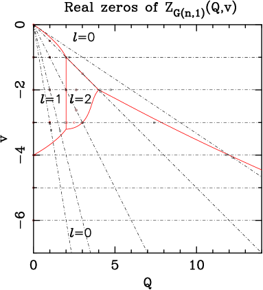
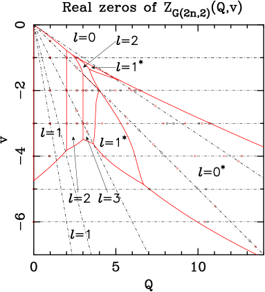
(a)	(b)
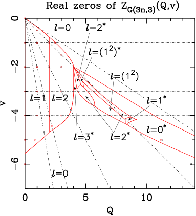
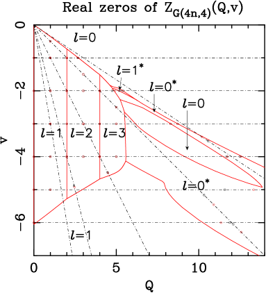
(c)	(d)

Figure 1: Real zeros of the Potts-model partition function and limiting curves $\mathcal{B}_{k}$ in the plane $(Q,v)$ for the generalized Petersen graphs $G(nk,k)$ with $k=1$ (a), $k=2$ (b), $k=3$ (c), and $k=4$ (d). For each panel, we show the real zeros along several lines (depicted as doted-dashed lines) of the type $Q=-pv$ ($p=1,2,3$), $v=-pQ$ ($p=1,2,3$), and $v=-1,-2,-3,-4,-5,-6$. For each value of $k$, the zeros correspond to the generalized Petersen graphs $G(9k,k)$ (black $\square$) and $G(10k,k)$ (red $\circ$). Each region is labeled with the sector the dominant eigenvalue belongs to (e.g., $\ell=1$). The asterisk in the sector label (e.g., $\ell=1^{*}$) means that there is a pair of complex-conjugate dominant eigenvalues in that region. The label $\ell=(1^{2})$ in panel (c) means that the dominant eigenvalue comes from the completely anti-symmetric irreducible representation $(1,1)=(1^{2})$ of $S_{2}$.

To study the partition-function zeros in this plane, we took several lines: $Q=-pv$, $v=-pQ$ (with $p=1,2,3$), and $v=-1,-2,\ldots,-6$. The line $v=-Q$ (resp. $v=-1$) corresponds to the flow-polynomial (resp. chromatic-polynomial) subspace. Along these lines, the two-variable partition function $Z_{G(nk,k)}(Q,v)$ reduces to a single-variable polynomial with integer coefficients. We then find its zeros by using the program MPSolve by Bini and Fiorentino [14, 15]. These lines are depicted as dot-dashed lines in Figures 1 and 2, and the zeros are also represented as circles and squares in the same figures. Although they exhibit some systematic features, these zeros are generally too scattered for any firm conclusions to be drawn.

A much better approach is to compute the limiting curves $\mathcal{B}_{k}$ when $n\to\infty$ in the $(Q,v)$ plane. We have used the direct–search method [46] to compute $\mathcal{B}_{k}$. But in some areas of the plane, this method did not work properly. The reason was that there are regions where the dominant eigenvalue is actually a pair of complex-conjugate eigenvalues belonging to the same sector. These regions are labeled by an asterisk in Figures 1 and 2.

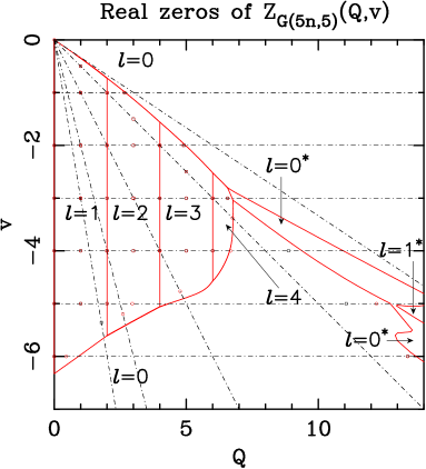
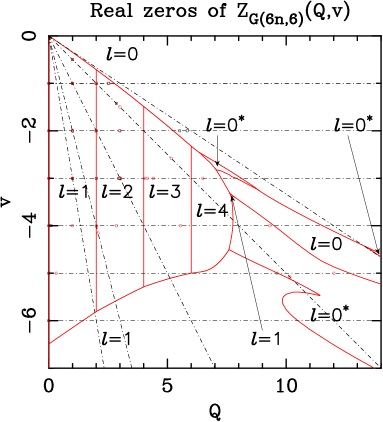
(a)	(b)
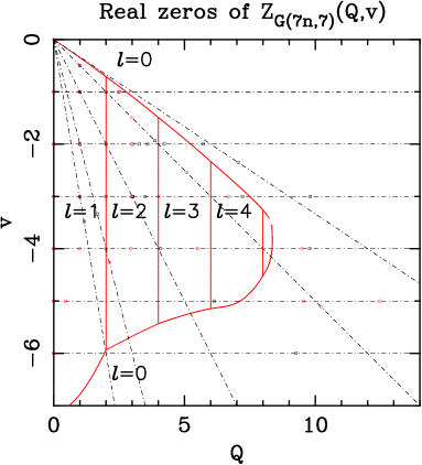
(c)

Figure 2: Real zeros of the Potts-model partition function and limiting curves $\mathcal{B}_{k}$ in the plane $(Q,v)$ for the generalized Petersen graphs $G(nk,k)$ with $k=5$ (a), $k=6$ (b), and $k=7$ (c). In (a) the zeros correspond to the generalized Petersen graphs $G(45,k)$ (black $\square$) and $G(50,k)$ (red $\circ$). For each value of $k$ in (b) and (c), the zeros correspond to the generalized Petersen graphs $G(3k,k)$ (black $\square$) and $G(4k,k)$ (red $\circ$). The rest of the notation is as in Figure 1. For $k=7$ we could not obtain the more involved structure for large $Q\mathrel{\hbox to0.0pt{\lower 3.0pt\hbox{$\mathchar 536\relax$}\hss}\raise 2.0pt\hbox{$\mathchar 318\relax$}}8.2$.

For $k=7,8,9,11$, even though we could not obtain the relevant transfer-matrix blocks, we were able to numerically compute (parts of) the corresponding limiting curves by using a code written in C. For $2\leq k\leq 6$ the result of this program coincides with the previous symbolic computation.

By looking at Figures 1 and 2, we see that for each fixed value of $k$ (with $1\leq k\leq 7$) there are two distinct regions in the corresponding phase diagram:

• This region is the closest to $Q=0$ and ends approximately at $Q\approx k+1$. It contains vertical lines at even integer values of $Q$, and has isolated limiting points at odd integer values of $Q$. It is bounded above and below by simple curves, and the dominant eigenvalues are simple ones, hence real valued. Close to $Q\mathrel{\hbox to0.0pt{\lower 3.0pt\hbox{$\mathchar 536\relax$}\hss}\raise 2.0pt\hbox{$\mathchar 318\relax$}}0$, the dominant eigenvalue belongs to the sector $\ell=1$, and every time we cross one of these vertical lines the value of $\ell$ increases by one unit.

• This region starts approximately at $Q\mathrel{\hbox to0.0pt{\lower 3.0pt\hbox{$\mathchar 536\relax$}\hss}\raise 2.0pt\hbox{$\mathchar 318\relax$}}k+1$, and it has a more involved structure. For $k=1$ there is a single outward branch starting at $(Q,v)=(4,-2)$ and extending to infinity. For $2\leq k\leq 6$, we find two boundary curves that extend outwards to infinity. Inside this region there are sub-regions where the dominant eigenvalue is actually a pair of complex-conjugate eigenvalues (in most cases they belong to the sector $\ell=0$). For $k=3$, we even find some regions where the dominant eigenvalue comes from the completely anti-symmetric representation $(1,1)\equiv(1^{2})$ of the $\ell=2$ sector (see Figure 1(c)).

Above [resp. below] both regions the dominant eigenvalue comes from the $\ell=0$ [resp. $\ell=(k+1)\bmod 2$] sector.

Region (a) looks qualitatively similar to the BK phase we have found for the 2D Potts models on the square and triangular lattices. Inside the region enclosed by the limiting curve $\mathcal{B}_{k}$, we find that for each integer $p\geq 0$ up to some maximum value $p_{\text{max}}$, there is a “phase” corresponding to an eigenvalue belonging to the fully symmetric representation $\lambda=(\ell)$ of $S_{\ell}$ with $\ell=p+1$ links. This phase contains all values of $Q$ in the interval $Q\in(2p,2p+2)$. Therefore, there are phase transitions at $Q=2p$ for $p\geq 0$ in an interval $(v_{-}(p),v_{+}(p))$, in which eigenvalues from the $\ell=p$ and $\ell=p+1$ become equimodular. As $k$ increases, the maximum value $p_{\text{max}}$ increases, so we find more phases in the BK phase. Even though $Q_{2}(-1)<3$ is rather small (see Section 7), as in the 2D case, we now find vertical lines at $Q$-values as large as $Q=8$ for $k=7$ ($p=4$), which is the maximum value of $k$ for which we have been able to produce the full “regular part”—region (a)—of the phase diagram.

We emphasize that the presence of vertical lines of limiting points extending from $v_{-}(Q)$ to $v_{+}(Q)$ provides clear evidence for the extent of the BK phase. In particular, the perfect verticality means that the temperature parameter $v$ is RG irrelevant for $v_{-}(Q)<v<v_{+}(Q)$, and the physics is thus controlled by an RG fixed point in the interior of the BK phase. Ideally one would like to corroborate the identification—and characterization—of the BK phase by verifying the algebraic decay of correlation functions inside the BK phase. In the 2D case this is a rather simple matter, since standard CFT results relate the strip free energies to critical exponents. In Section 4.3 we pursue a more modest goal, namely to give numerical evidence that the correlation length $\xi$ is proportional to $k$ inside the BK phase and tends to a constant outside it. Since $k$ roles as the effective width in the strip geometry underlying the transfer matrix formalism, this implies that the BK phase is characterized by $\xi\to\infty$ in the thermodynamic limit $k\to\infty$, and so is critical indeed.

In the phase characterized by $\ell$ links, corresponding to the interval $Q\in(2(\ell-1),2\ell)$, the amplitude corresponding to the fully symmetric representation $\lambda=(\ell)$ is [cf., (3.4)] [24, 30]

$$\alpha_{\ell,(\ell)}\;=\;\frac{1}{\ell!}\,(Q-2\ell+1)\,\prod\limits_{i=0}^{\ell-2}(Q-i)\,.$$ (4.1)

Therefore, it vanishes at the mid-point $Q=2\ell-1$ of the above interval; hence, this is an isolated limiting point.

Remark. Notice that the families $G(n,1)$ and $G(2n,2)$ are planar. Indeed, in Figures 1(a)–(b), we see that there are isolated limiting points at the non-integer value $Q=B_{5}$ in agreement with the Beraha conjecture. This can be explained by the fact that the amplitude for the $\ell=2$ sector is not the generic one, but $\gamma_{2}$ for $k=1$, and $\beta_{2}$ for $k=2$. (cf., [30, Eq. (3.28)]). Indeed, both amplitudes are equal to $\beta_{2}=\gamma_{2}=Q^{2}-3Q+1$, and $\beta_{2}(B_{5})=0$, as expected.

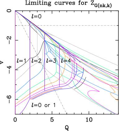
Figure 3: Limiting curves $\mathcal{B}_{k}$ in the plane $(Q,v)$ for the generalized Petersen graphs $G(nk,k)$ with $k=1$ (black), $k=2$ (gray), $k=3$ (light blue), $k=4$ (green), $k=5$ (orange), $k=6$ (pink), $k=7$ (violet), $k=8$ (red), $k=9$ (navy blue), and $k=11$ (black). We label some regions with the sector to which the dominant eigenvalue (for large enough $k$) belongs (e.g., $\ell=3$). The horizontal $v=-1$ (resp. inclined $v=-Q$) dot-dashed line corresponds to the chromatic (resp. flow) polynomial subspace.

Figure 3 shows all the limiting curves put together. If we look at the bottom part of these curves ($Q=0,v\mathrel{\hbox to0.0pt{\lower 3.0pt\hbox{$\mathchar 536\relax$}\hss}\raise 2.0pt\hbox{$\mathchar 316\relax$}}-4$), the value of $k$ increases as we move outwards. We notice the following empirical observations:

• As $k$ increases, the BK phase enlarges and more $\ell$ sectors are visible in the unphysical region.

• The upper boundary curve converges quickly to a limit. In particular, its slope at $Q=0$ seems to be equal to $-1/3$. Its crossing with the horizontal line $v=-1$ (depicted as dot-dashed line in Figure 3) defines the value of $Q_{2}(-1)$. (See Section 7.) We can identify this curve with the AF critical curve $v_{+}(Q)$ for this model.

• The lower boundary curve $v_{-}(Q)$ converges slowly to some limit. The inclined dot-dashed line in Figure 3 corresponds to the flow polynomial. The convergence is not as fast as for $Q_{2}(-1)$. (See Section 6).

• Using the rough estimates for the limiting curves for $k=9,11$, we see that $Q_{\text{max}}\mathrel{\hbox to0.0pt{\lower 3.0pt\hbox{$\mathchar 536\relax$}\hss}\raise 2.0pt\hbox{$\mathchar 318\relax$}}9.4$, which is far larger than the maximum value $Q_{\text{max}}=4$ obtainable for 2D Potts models with either cyclic and toroidal boundary conditions. We can obtain a more accurate estimate of $Q_{\text{max}}$ by looking at the line $v=-4$ (see Figures 1–2). This line seems to cross the “regular” part of the BK phase at its more distant point from the origin, and has the nice property that the eigenvalue that is dominant on the high-$Q$ side of the crossing comes always from the $\ell=0$ sector for all values of $k$ we can access numerically: i.e., $3\leq k\leq 10$. These results are displayed in Table 1. As a prevention against parity effects, we have fitted the odd– and even–$k$ data subsets separately. We have used several Ansätze: i.e., power law and polynomials of different degrees in $1/k$. From the dispersion of the estimates for $Q_{\text{max}}$, we conclude that our preferred estimate is $Q_{\text{max}}\mathrel{\hbox to0.0pt{\lower 3.0pt\hbox{$\mathchar 536\relax$}\hss}\raise 2.0pt\hbox{$\mathchar 318\relax$}}12.4(1)$, as the limiting value of the crossings along the line $v=-4$ only provides a lower bound for the true $Q_{\text{max}}$.

  $k$	$Q_{c}(k)$
  3	3.5918146982
  4	5.5837328676
  5	6.6418204973
  6	7.7533996189
  7	8.3495427730
  8	8.8740090544
  9	9.2660844176
  10	9.5702423022

  Table 1: Values of $Q_{c}(k)$ along the line $v=-4$ for the generalized Petersen graphs $G(nk,k)$ for $3\leq k\leq 10$.

4.3 Criticality of the Berker–Kadanoff phase

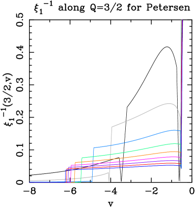
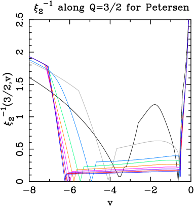
(a)	(b)
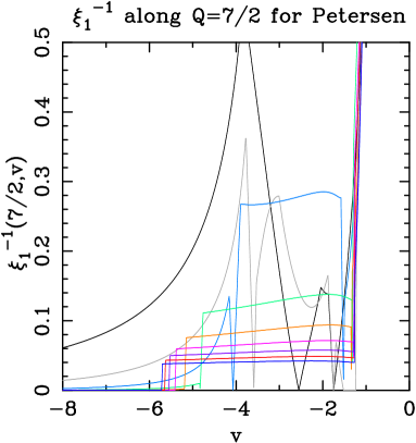
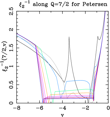
(c)	(d)

Figure 4: Inverse correlation lengths $\xi_{i}^{-1}(Q,v)$ for $Q=3/2$ (a,b), and $Q=7/2$ (c,d). The index $i=1$ (resp. $i=2$) corresponds to the the ratio of the first (resp. second) sub-dominant eigenvalue and the dominant one [cf., (4.2)]. We show the inverse correlation lengths $\xi_{i}^{-1}$ ($i=1,2$) for the Petersen graphs $G(nk,k)$ with $k=1$ (black), $k=2$ (gray), $k=3$ (light blue), $k=4$ (green), $k=5$ (orange), $k=6$ (pink), $k=7$ (violet), $k=8$ (red), and $k=9$ (navy blue).

The BK phase in 2D Potts models is a critical phase: it corresponds to a massless phase with algebraic decaying of correlations. In this section we want to study whether the BK phase for the non-planar Petersen graphs $G(nk,k)$ is critical or not. One way to achieve this goal is to consider the inverse correlation length (or mass gap) given by the ratios

$$\xi_{i}^{-1}(Q,v)\;=\;\log\left|\frac{\mu_{i}(Q,v)}{\mu_{*}(Q,v)}\right|\,,$$ (4.2)

where $\mu_{*}$ is the dominant eigenvalue, and $\mu_{i}$ with $i=1,2,\ldots$ is the $i$-th subdominant eigenvalue (i.e., $|\mu_{*}|\geq|\mu_{1}|\geq|\mu_{2}|\geq\ldots$). In Figure 4 we have shown the values of $\xi_{i}^{-1}$ for $i=1,2$ versus the parameter $v$ at fixed values of $Q=3/2,7/2$. Note that for $Q=3/2$ we cross the region of the BK phase dominated by the $\ell=1$ sector, while for $Q=7/2$, we cross the nearby region dominated by the $\ell=2$ sector. We expect to find a disordered phase for $v\in(v_{+}(Q),0]$, the BK phase for $v\in(v_{-}(Q),v_{+}(Q))$, and another phase for $v<v_{-}(Q)$. The critical/non-critical nature of the last two phases needs to be determined.

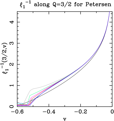
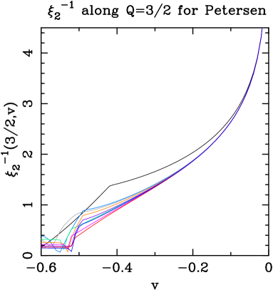
(a)	(b)

Figure 5: Zoom-out of Figures 4(a,b) showing the inverse correlation lengths $\xi_{i}^{-1}(Q,v)$ for $Q=3/2$ and $i=1$ (a) and $i=2$ (b) for the Petersen graphs $G(nk,k)$. The color code is as in Figure 4. We show in both panels the curves for $1\leq k\leq 9$.

Let us now start with the first region $v\in(v_{+}(Q),0]$. Figure 4 does not give much information about this regime; so we provide a zoom of this region in Figure 5 for $Q=3/2$. Now the behavior of the different curves as $k$ increases is clear: they tend to some finite limit $\xi^{-1}_{1,\infty}(v)>0$. This limit curve is essentially attained for $k\geq 3$ and $v\mathrel{\hbox to0.0pt{\lower 3.0pt\hbox{$\mathchar 536\relax$}\hss}\raise 2.0pt\hbox{$\mathchar 318\relax$}}-0.3$. We conclude that in this region there is a finite gap in the thermodynamic limit, and therefore, this is a non-critical phase. For $Q=5/2$ the plots are very similar. To summarize, the region $v\in(v_{+}(Q),0]$ is a non-critical (disordered) phase.

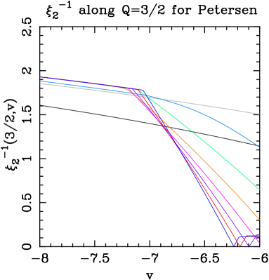
(a)	(b)

Figure 6: Zoom-out of Figures 4(a,b) showing the inverse correlation lengths $\xi_{i}^{-1}(Q,v)$ for $Q=3/2$ and $i=1$ (a) and $i=2$ (b) for the Petersen graphs $G(nk,k)$. The color code is as in Figure 4. We show in both panels the curves for $1\leq k\leq 9$.

Let us now consider the last region $v\in(-\infty,v_{-}(Q))$. The most relevant part of this regime is displayed in Figure 6 for $Q=3/2$. The plot of $\xi_{1}^{-1}$ displayed in Figure 6(a) show clearly that this inverse correlation length tends to zero as $k$ increases. Therefore, one could naively conclude that this also a massless phase. There are two almost identical eigenvalues, one coming from the $\ell=0$ sector, and the other from the $\ell=1$ sector. But the plot of $\xi_{2}^{-1}$ in Figure 6(b) show that the second correlation length is finite. For $k\geq 4$ and $v\mathrel{\hbox to0.0pt{\lower 3.0pt\hbox{$\mathchar 536\relax$}\hss}\raise 2.0pt\hbox{$\mathchar 318\relax$}}7.2$ all curves collapse almost perfectly. Therefore, we expect that as $k$ tends to infinity, these curves will tend to some finite limit $\xi_{2,\infty}^{-1}(v)>0$. The plots for $Q=5/2$ are very similar. Therefore we conclude that the region $v\in(-\infty,v_{-}(Q))$ is also a non-critical phase. The two most dominant eigenvalues for finite values of $k$ will tend to a common function, so the mass gap in this phase is given in the thermodynamic limit by $\xi_{2,\infty}^{-1}$.

Finally, we focus on the BK phase $v\in(v_{-}(Q),v_{+}(Q))$. Figure 4 shows that in this region the curves $\xi_{i}^{-1}$ are rather flat around some non-zero value for $k\geq 3$, and as $k$ increases, this value becomes smaller. This is an indicator that as $k$ increases the mass gap tends to zero in this phase. Therefore, we expect that this is a critical (massless) phase (as for the 2D Potts model). In 2D models, CFT predicts that the mass gap for a critical theory defined on a strip graph of width $L$ and cylindrical boundary conditions behaves like $\xi_{i}^{-1}=A_{i}/L+o(L^{-1})$, where $A_{i}$ is a universal constant, proportional to the critical exponent that governs the algebraic decay of an appropriate correlation function. For the non-planar recursive strip graphs studied here, there is no such strong link to CFT, but it is nevertheless true that $k$ roles as the effective width of the strip in the transfer matrix formalism [30]. Critical behavior will therefore result if the mass gap for the non-planar Petersen graphs $G(nk,k)$ behaves asymptotically like $1/k$. To determine whether this is the case, we have plotted in Figure 7 the quantity $k\,\xi_{i}^{-1}$ versus $v$ for fixed values of $Q=3/2,7/2$.

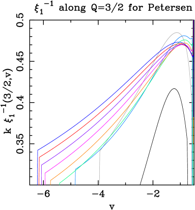
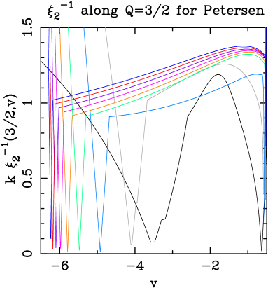
(a)	(b)
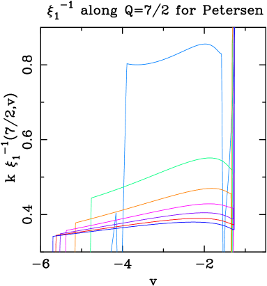
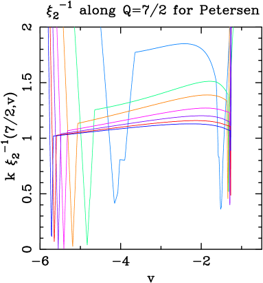
(c)	(d)

Figure 7: Zoom-out of Figure 4 showing $k$ times the inverse correlation length, $k\xi_{i}^{-1}(Q,v)$, with $Q=3/2$ (a,b) and $Q=7/2$ (c,d) for the Petersen graphs $G(nk,k)$ in the region $v\in(v_{-}(Q),v_{+}(Q))$ for $i=1$ (a,c) and $i=2$ (b,d). For $Q=3/2$, we show in panels (a,b) the curves for $1\leq k\leq 9$. For $Q=7/2$, we only show in panels (c,d) those curves with $3\leq k\leq 9$, as for smaller values of $k$ the line $Q=7/2$ crosses the limiting curves $\mathcal{B}_{k}$ at their non-regular part. The color code is as in Figure 4.

Even though there are obvious finite-size effects, for $Q=3/2$ it looks like the curves tend to some limiting curve from below. However, for $Q=7/2$, this convergence is from above. This means that there is a change of sign in the dominant finite-size-scaling correction term. The best convergence is clearly attained for $Q=7/2$ and $i=1$. We have tried to fit the data for $Q=3/2$ and $7/2$ and $i=1,2$ to an Ansatz

$$k\xi_{i}^{-1}(Q,v)\;=\;g_{i}(Q,v)+\frac{h_{i}(Q,v)}{k}\,,$$ (4.3)

where the second term intends to mimic the finite-size-scaling corrections. For the four cases we have considered here, we find reasonable fits leading to smooth functions $g_{i}(Q,v)$ as functions of $v$. Therefore, we conjecture that in the BK phase

$$\xi_{i}^{-1}(Q,v)\;=\;\frac{g_{i}(Q,v)}{k}+o(k^{-1})\,.$$ (4.4)

This implies that the BK phase is critical in the sense that it is massless. This coincides with the properties of the BK phase found for 2D Potts models.

In Section 4.2, we have shown that the limiting curves $\mathcal{B}_{k}$ contained vertical lines for even integer values of $Q=0,2,\ldots$ and $v$ in the interval $v\in(v_{-}(Q),v_{+}(Q))$. The perfect verticality of these lines implies that the temperature is an irrelevant operator in the RG sense. Moreover, in Section 4.3, we have shown that inside the region $v\in(v_{-}(Q),v_{+}(Q))$ for fixed values of $Q$, the mass gap vanishes in the infinite-$k$ limit. This implies that this region is critical. Therefore, both conditions that define the BK phase (as we know from 2D Potts models) are met also for the $Q$-state Potts model on the Petersen graphs $G(nk,k)$.

We conclude that the BK phase exists also at least for recursive families of non-planar graphs, and a role analogous to the one played by the Beraha numbers for planar graphs is now played by the non-negative integers for non-planar graphs. The natural question is to know, in the non-planar case, whether there are also cancellations among eigenvalues and vanishing of amplitudes when $Q$ is a non-negative integer. This question will be answered in the next section.

5 What happens for integer values of $\bm{Q}$?

In this section we will consider the partition function for the generalized Petersen graphs $Z_{G(nk,k)}(Q,v)$ when $Q$ takes a non-negative integer value.

Let us fix $k\geq 3$. For each $0\leq\ell\leq k$, let us denote by $\mathcal{E}_{\ell}$ the set of non-trivial eigenvalues $\mu_{k,\ell,\lambda,s}$ associated to the sector of $\ell$ links. Moreover, let $\mathcal{E}_{k+1}$ be the one-element set containing only the trivial eigenvalue $\mu_{k,k+1}=v^{2k}$. In the same way, let $\mathcal{E}_{\ell,\lambda}$ denote the set of non-trivial eigenvalues $\mu_{k,\ell,\lambda,s}$ corresponding to the irreducible representation $\lambda$ of the group $S_{\ell}$.

When $Q$ is a non-negative integer, some of the non-trivial eigenvalues of ${\sf T}_{k+1,\ell,\lambda}^{(nt)}$ (for $0\leq\ell\leq k-1$) or ${\sf T}_{k+1,k}^{(nt)}$ (for $\ell=k$) may reduce to the trivial eigenvalue $\mu_{k,k+1}=v^{2k}$. These eigenvalues are excluded by definition from the sets $\mathcal{E}_{\ell}$ and $\mathcal{E}_{\ell,\lambda}$ defined above for $0\leq\ell\leq k$.

Finally, let us denote by $\chi_{k,\ell,\lambda}$ the net non-trivial contribution to the partition function $Z_{G(nk,k)}$ [cf., (3.9)] of the sector with $\ell$ links and the irreducible representation $\lambda$ of $S_{\ell}$:

$$\chi_{k,\ell,\lambda}\;=\;\left.\sum_{s}\right.^{\prime}\mu_{k,\ell,\lambda,s}^{n}\,.$$ (5.1)

The prime on the sum in the r.h.s. of (5.1) means that we exclude, for a particular non-negative integer value of $Q$, both 1) those non-trivial eigenvalues of ${\sf T}_{k+1,\ell,\lambda}^{(nt)}$ that become identical to the trivial one $v^{2k}$, and 2) those eigenvalues in $\mathcal{E}_{\ell,\lambda}$ that are exactly canceled by the contribution of other sectors. For $\ell=k$, we use the eigenvalues $\mu_{k,k}$ of the reduced matrix ${\sf T}_{k+1,k}^{(nt)}$ instead, and $\lambda$ plays no role. For $\ell=0,1$, the sub-index $\lambda$ is also superfluous and can be dropped.

We can obtain the eigenvalues of each transfer matrix ${\sf T}_{k+1,\ell,\lambda}$ by computing its characteristic polynomial symbolically using Mathematica. This procedure can be carried out for $k=2,3,4$; but for $k=5$, this is not feasible due to the large dimension of some of the transfer matrices. We have observed that the characteristic polynomials obtained in this way cannot be factorized over the integers. (This is not true in general when $Q$ takes integer values, as shown below.) Indeed, if we find that two transfer matrices have characteristic polynomials with a common factor, then we can deduce that the eigenvalues coming from the common factor appear in both matrices. On the contrary, if the characteristic polynomials of two transfer matrices have no common factor, then they do not contain any common eigenvalue. For $k=5$ we have numerically computed the eigenvalues to high precision (i.e., 100 digits) using Mathematica. For these cases, we could check the conjectures obtained from the smaller values for $k$.

We summarize our findings for the smallest integer values by using the exact results for $k=3,4,5$ (which correspond to non-planar generalized Petersen graphs).

5.1 $\bm{Q=0}$

This case is trivial, as $Z_{G}(0,v)=0$ for any graph with at least one vertex. Therefore, there should be a massive cancellation of eigenvalues and amplitudes, so that the net sum is always zero.

First of all, it is clear from (3.4), that only the fully anti-symmetric representations of $S_{\ell}$ give a non-zero contribution. In fact, if we represent by $(1^{\ell})$, the fully anti-symmetric representation of $S_{\ell}$, then

$$\alpha_{\ell,(1^{\ell})}(0)\;=\;(-1)^{\ell}\,.$$ (5.2)

The two non-generic amplitudes are also [30]:

$$\beta_{k}(0)\;=\;\gamma_{k}(0)\;=\;(-1)^{k}\,.$$ (5.3)

We find that $\mathcal{E}_{0}\subset\mathcal{E}_{1}$: i.e., the set of $\ell=0$ eigenvalues is a proper subset of those of the next sector. For the higher sectors (except the last one), we find that $\mathcal{E}_{\ell}\setminus\mathcal{E}_{\ell-1}\subset\mathcal{E}_{\ell+1}$. In words, the non-trivial eigenvalues of the sector with $\ell$ links that do not belong to the sector with $\ell-1$ links, are a proper subset of the set of non-trivial eigenvalues of the sector with $\ell+1$ links. The last step corresponds to $\ell=k$, and it reads $\mathcal{E}_{k}\setminus\mathcal{E}_{k-1}=\varnothing$. (Recall that $\mathcal{E}_{\ell}$ for $0\leq\ell\leq k$ contains non-trivial eigenvalues, while $\mathcal{E}_{k+1}$ contains the trivial eigenvalue $v^{2k}$.)

When $Q=0$, some of the eigenvalues $\mu_{k,\ell,\lambda}$ in (3.9) reduce to the trivial one $\mu_{k,k+1}=v^{2k}$. These new trivial eigenvalues appear with some multiplicity $n_{k,\ell}>0$ in sectors $1\leq\ell\leq k$ (resp. $2\leq\ell\leq k$) for odd (resp. even) values of $k$ (e.g., when $k=4$, $n_{4,2}=n_{4,3}=3$, and $n_{4,4}=1$). But their net contribution always cancels the last term on the r.h.s. of Eq. (3.9):

$$\sum\limits_{\ell=1}^{k}n_{k,\ell}\,(-1)^{\ell}+\gamma_{k+1}(0)\;=\;0\,.$$ (5.4)

The above inclusion-exclusion patterns, in addition to the values taken by the amplitudes, imply that all eigenvalues cancel out exactly, giving the expected result $Z_{G(nk,k)}(0,v)=0$.

5.2 $\bm{Q=1}$

This case is also trivial, as for any graph $G=(V,E)$, $Z_{G}(1,v)=(1+v)^{|E|}$. This comes from the FK representation (1.3) of the $Q$-state Potts model. Recall that for the generalized Petersen graph $G(nk,k)$, $|E|=3nk$.

The generic amplitudes $\alpha_{\ell,\lambda}(1)$ are non-zero only for the following cases:

• $\ell=0$ with $\alpha_{0}=1$.

• $\ell=2$ and the representation $(2)$ with $\alpha_{2,(2)}=-1$.

• For each $\ell\geq 3$, the representation $(2,1^{\ell-2})$, with $\alpha_{\ell,(2,1^{\ell-2})}=(-1)^{\ell-1}$.

The non-generic amplitudes [30] take the values

$$\beta_{k}\;=\;(k-1)(-1)^{k-1}\,,\qquad\gamma_{k+1}\;=\;(-1)^{k}\,.$$ (5.5)

The pattern for the non-trivial eigenvalues is as follows: For $\ell=0$, we have the decomposition $\mathcal{E}_{0}=\{\mu_{0}\}\cup\mathcal{E}^{\prime\prime}_{0}$, with $\mu_{0}=(1+v)^{3k}$. Then an inclusion-exclusion pattern similar to the $Q=0$ case occurs: $\mathcal{E}^{\prime\prime}_{0}\subset\mathcal{E}_{2}$, $\mathcal{E}_{\ell}\setminus\mathcal{E}_{\ell-1}\subset\mathcal{E}_{\ell+1}$ for $3\leq\ell\leq k-1$, and $\mathcal{E}_{k}\setminus\mathcal{E}_{k-1}=\varnothing$.

There is a slight difference with the $Q=0$ case: the non-zero amplitude for $\ell=k$ is $(k-1)(-1)^{k-1}$, so that the corresponding (non-trivial) eigenvalues in $\mathcal{E}_{k}$ contribute to the partition function with this amplitude. But these eigenvalues also appear in the preceding sector $\ell=k-1$ with a degeneracy exactly equal to $k-1$; therefore, these two contributions cancel out in the partition function.

The trivial eigenvalue $v^{2k}$ cancels out in all cases $3\leq k\leq 5$. Unfortunately, we have been unable to find a simple pattern for the multiplicities and the amplitudes in this case.

Therefore, all eigenvalues cancel out exactly, except the simple eigenvalue $\mu_{0}=(1+v)^{3k}$ coming from the $\ell=0$ sector. This eigenvalue gives the right value of the partition function when $Q=1$. Using (5.1), we can write the partition function as

$$Z_{G(nk,k)}(1,v)\;=\;\chi_{k,0}\;=\;(1+v)^{3nk}\,.$$ (5.6)

5.3 $\bm{Q=2}$

This case corresponds to the Ising model on the family of graphs $G(nk,k)$. The generic amplitudes $\alpha_{\ell,\lambda}(2)$ (3.4) are non-zero only for the following cases:

• $\ell=0$ with $\alpha_{0}=1$.

• $\ell=1$ with $\alpha_{1}=1$.

• $\ell=2$ and the representation $(2)$ with $\alpha_{2,(2)}=-1$.

• $\ell=3$ and the representation $(3)$ with $\alpha_{3,(3)}=-1$.

• For each $\ell\geq 4$ and the representations $(3,1^{\ell-3})$ and $(2^{2},1^{\ell-4})$, with $\alpha_{\ell,(3,1^{\ell-3})}=\alpha_{\ell,(2^{2},1^{\ell-4})}=(-1)^{\ell}$.

The non-generic amplitudes take the values [30]:

$$\beta_{k}\;=\;(k^{2}-3k+1)(-1)^{k}\,,\qquad\gamma_{k+1}\;=\;-1\,.$$ (5.7)

The pattern for the non-trivial eigenvalues is more involved than for the previous cases. In the sector $\ell=0$, we find two types of non-trivial eigenvalues: $\mathcal{E}_{0}=\mathcal{E}^{\prime}_{0}\cup\mathcal{E}^{\prime\prime}_{0}$. The first sub-set contains $|\mathcal{E}^{\prime}_{0}|=2^{k}$ eigenvalues, and these eigenvalues do contribute to the partition function $Z_{G(nk,k)}(2,v)$. The second subset is contained in $\mathcal{E}_{3}$ ($\mathcal{E}^{\prime\prime}_{0}\subset\mathcal{E}_{3}$); but the amplitudes of these two sectors are equal in absolute value with distinct signs, so they give a zero net contribution to $Z_{G(nk,k)}(2,v)$. In the sector $\ell=1$, a similar phenomenon occurs: $\mathcal{E}_{1}=\mathcal{E}^{\prime}_{1}\cup\mathcal{E}^{\prime\prime}_{1}$, with $|\mathcal{E}^{\prime}_{1}|=2^{k}$ contributing eigenvalues, and the rest cancel out with part of the $\ell=2$ sector: $\mathcal{E}^{\prime\prime}_{1}\subset\mathcal{E}_{2}$. The non-trivial eigenvalues in $\mathcal{E}_{2}\setminus\mathcal{E}^{\prime\prime}_{1}$ and $\mathcal{E}_{3}\setminus\mathcal{E}^{\prime\prime}_{0}$ also appear in the higher sectors $\ell\geq 4$, and their net contribution is always zero. We also find for $k=4,5$ and sector $\ell=k$, $2k+1$ distinct eigenvalues with amplitude $\beta_{k}$. The same $2k+1$ non-trivial eigenvalues also appear at lower sectors with multiplicities that make the their net contribution equal to zero.

The trivial eigenvalue $v^{2k}$ cancels out in all cases $3\leq k\leq 5$. But its pattern does not look simple, and probably has parity effects.

Therefore, all eigenvalues cancel out exactly, except the $2^{k+1}$ eigenvalues in the set $\mathcal{E}^{\prime}_{0}\cup\mathcal{E}^{\prime}_{1}$. This is expected, as on each layer of $G(nk,k)$ there are exactly $k+1$ vertices, and hence the corresponding transfer matrix in the spin representation has dimension $2^{k+1}$. Therefore, the partition function reads:

$$Z_{G(nk,k)}(2,v)\;=\;\chi_{k,0}+\chi_{k,1}\,,$$ (5.8)

where each $\chi_{k,\ell}$ contains $2^{k}$ non-zero eigenvalues. This formula looks like the expression found for the RSOS representation of the 2D Ising model [26].

5.4 $\bm{Q=3}$

The situation is now more involved, but the result is rather simple:

$$Z_{G(nk,k)}(3,v)\;=\;\chi_{k,0}+2\chi_{k,1}+\chi_{k,2,(1^{2})}\,,$$ (5.9)

where there are $\lfloor 3^{k}/2\rfloor$+1, $3^{k}$, and $\lfloor 3^{k}/2\rfloor$ non-zero eigenvalues in the above “characters”, respectively. In total, there are $2\times 3^{k}$ contributing eigenvalues in the set $\mathcal{E}^{\prime}_{0}\cup\mathcal{E}^{\prime}_{1}\cup\mathcal{E}^{\prime}_{2}$, where we have split each eigenvalue set $\mathcal{E}_{k}=\mathcal{E}^{\prime}_{k}\cup\mathcal{E}^{\prime\prime}_{k}$, as in the case $Q=2$. The final formula resembles the formula found for the RSOS representation of the 3–state Potts model in 2D [26].

We also find for $k=4,5$ the following patterns for the other eigenvalues (whose net contribution to $Z_{G(nk,k)}(3,v)$ cancels out): in the sector $\ell=1$, $\mathcal{E}_{1}\setminus\mathcal{E}^{\prime}_{1}\subset\mathcal{E}_{3,(3)}$. In the sector $\ell=2$, the only non-vanishing amplitude is $\alpha_{2,(1^{2})}=1$, while for sector $\ell=3$, there are two non-zero amplitudes $\alpha_{3,(3)}=-2$ and $\alpha_{3,(2,1)}=-1$. We then find that $\mathcal{E}_{2}\setminus\mathcal{E}^{\prime}_{2}\subset\mathcal{E}_{3,(2,1)}$. Let us note that $Q=3$ is inside the phase characterized by $\ell=2$ links; but from this sector most eigenvalues cancel out.

The trivial eigenvalue $v^{2k}$ cancels out in all cases $3\leq k\leq 5$. But its pattern does not look simple, and probably has again parity effects.

5.5 $\bm{Q=4}$

The analysis of the eigenvalues for $Q=4$ is more complicated (in fact, for $k=3$ we do not find any cancellation at all!). For $k=4,5$ we do find cancellations; in particular, all eigenvalues associated to negative generic amplitudes $\alpha_{\ell,\lambda}$ cancel out, so that we conjecture the following formula:

$$Z_{G(nk,k)}(4,v) = \chi_{k,0}+3\chi_{k,1}+2\chi_{k,2,(2)}+3\chi_{k,2,(1^{2})}+\chi_{k,3,(1^{3})}$$ (5.10)

$$\qquad+Av^{2kn}I[\text{$k$ even}]\,,$$

where $I[A]$ is the indicator function for the event $A$ ($I[A]=1$ if $A$ is true, and zero, otherwise). We cannot determine the value of the constant $A$ (or even if it is really a constant), as we only have one data point ($k=5$).

The non-trivial eigenvalues associated to $\ell=3$ and $\lambda=(3)$ (with $\alpha_{3,(3)}=-2$) cancel out with those appearing in $\mathcal{E}_{2,(2)}$: i.e., $\mathcal{E}_{3,(3)}\subset\mathcal{E}_{2,(2)}$. For $k=5$, we find $11$ distinct eigenvalues for $\ell=k$. These eigenvalues appear also for $(\ell,\lambda)=(1,(1)),(4,(3,1)),(4,(2,1^{2}))$; and their net contribution is zero. The other 305 eigenvalues that appear in $\mathcal{E}_{4,(3,1)}$ (resp. $\mathcal{E}_{4,(2,1^{2})}$) cancel with those appearing in $\mathcal{E}_{2,(1^{2})}$ (resp. $\mathcal{E}_{3,(1^{3})}$). In summary, all eigenvalues associated to negative amplitudes cancel out (except the trivial one for even values of $k$), and there are only five non-trivial contributions to the partition function. (Indeed, this is in sharp contrast with the infinite sum obtained using the RSOS representation for the 4-state Potts model on a planar graph [26]).

5.6 Conjectured behavior for integer $\bm{Q}$

The above results for $Q=0,1,2,3,4$ suggest the following conjecture for the partition function of the generalized Petersen graphs $Z_{G(nk,k)}(Q,v)$ (3.6) when $Q$ takes a non-negative integer value.

Conjecture 5.1

Let us fix $Q$ to a non-negative integer value $N$. Then the partition function of the generalized Petersen graphs (3.6) reduces for any $k\geq N$ to:

$$Z_{G(nk,k)}(N,v)\;=\;\sum\limits_{\ell=0}^{N-2}\left[\sum\limits_{00112233\begin{array}[]{c}\lambda\in S_{\ell}\\ \alpha_{\ell,\lambda}(N)>0\end{array}}\alpha_{\ell,\lambda}\,\chi_{k,\ell,\lambda}\right]\;+\;\chi_{k,N-1,(1)^{N-1}}+\rho_{k}(N)v^{2nk}\,,$$ (5.11)

where we have defined the “characters” $\chi_{k,\ell,\lambda}$ in (5.1), $\rho_{k}$ is the number of the trivial eigenvalue contributes to the partition function, and the second sum is over all irreducible representations $\lambda\in S_{\ell}$ with a positive value of the amplitude $\alpha_{\ell,\lambda}$ at $Q=N$.

Remarks. 1. Notice that $\alpha_{N-1,(1)^{N-1}}=1$.

2. The function $\rho_{k}(N)$ is simple for small values of $0\leq N\leq 4$:

$$\rho_{k}(N)\;=\;\begin{cases}0&\quad\text{if $0\leq N\leq 3$}\\ 6\,I[\text{$k$ even}]&\quad\text{if $N=4$}\end{cases}$$ (5.12)

3. For any $k\geq N$, we find the following sum rule:

$$\sum\limits_{\ell=0}^{N-1}\alpha_{\ell,\lambda}\widetilde{N}_{k}(\ell,\lambda)+\rho_{k}(N)\;=\;N^{k+1}\,,$$ (5.13)

where $\widetilde{N}_{k}(\ell,\lambda)$ is the number of contributing non-trivial eigenvalues to the partition function $Z_{G(nk,k)}(N,v)$ and coming from the sector with $\ell$ links and the representation $\lambda\in S_{\ell}$. Note that (5.13) is compatible with the fact that, for $Q$ integer, the transfer matrix can alternatively be represented in terms of Potts spins. In this representation the partition function with periodic longitudinal boundary conditions is an ordinary matrix trace, and no eigenvalue cancellations can take place. Therefore, the number of eigenvalues (counted with multiplicities) is $Q^{k+1}$ indeed.

6 Flow polynomial for the generalized Petersen graphs

In Ref. [30] we focused on the particular case of the flow polynomial of the generalized Petersen graphs $G(nk,k)$ for $1\leq k\leq 7$. Using the eigenvalues found there, our present goal is to compute the accumulation sets of flow zeros in the limit $n\to\infty$. In particular we consider the limiting curves $\mathcal{B}_{k}$ for $1\leq k\leq 7$. We have computed these curves for $k=1,2,\ldots,7$ using the direct-search method, as described in [46]. The results are shown in Figures 8 and 9 in the complex $Q$-plane.

We have noticed several empirical patterns in Figures 8 and 9. The first one is related to the number of outward branches of the limiting curve $\mathcal{B}_{k}$, and the dominant eigenvalue in each asymptotic sector:

Conjecture 6.1

Fix $k\geq 1$. Then, the limiting curve $\mathcal{B}_{k}$ has exactly $2k$ outward branches extending to $Q=\infty$, with asymptotic angles $\arg Q=\theta_{k,j}$ where

$$\theta_{k,j}\;=\;\left(j-\frac{1}{2}\right)\frac{\pi}{k}\,,\qquad\text{for $j=1,\ldots,2k$.}$$ (6.1)

Moreover, the dominant eigenvalue is $\mu_{k+1,0,\star}$ in the asymptotic regions

$$\theta_{k,j}\;\leq\;\arg Q\;\leq\;\theta_{k,j+1}\quad\text{for}\quad\begin{cases}\;j=1,3,\ldots,2k-1&\text{if $k$ is even}\\ \;j=2,4,\ldots,2k&\text{if $k$ is odd}\end{cases}$$ (6.2)

while in the other asymptotic sectors the dominant eigenvalue is $\mu_{k+1,1,(1),\star}$.

We may also conjecture that, as $k\to\infty$, the limiting curves $\mathcal{B}_{k}$ (without the outward branches) converge to some curve $\mathcal{B}_{\infty}$. This is what Figure 10 suggests. Indeed, outside this curve, the outward branches seem to get denser as $k$ increases. Therefore, we conjecture that the set of accumulation points of the flow–polynomial zeros for the generalized Petersen graphs $G(nk,k)$ is dense in the whole complex $Q$-plane, except in the interior of the curve $\mathcal{B}_{\infty}$. If this conjecture is true, it implies in particular that flow roots of non-planar cubic graphs are dense in the complex plane, except possibly in some bounded region near the origin. Note that a similar result holds (by duality) for the flow roots of planar graphs [53], but without the restriction to cubic graphs.

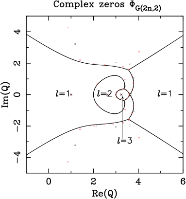
(a)	(b)
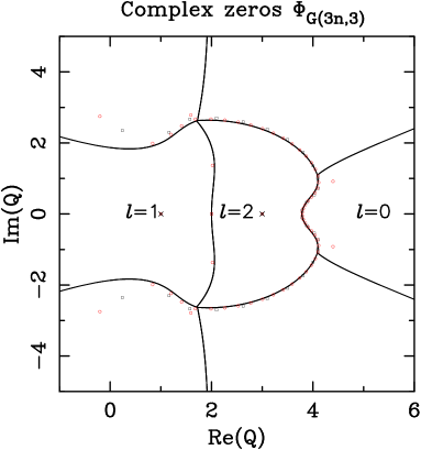
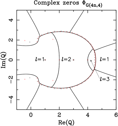
(c)	(d)

Figure 8: Complex zeros of the flow polynomial and limiting curves $\mathcal{B}_{k}$ in the complex $Q$–plane for the generalized Petersen graphs $G(nk,k)$ with $k=1$ (a), $k=2$ (b), $k=3$ (c), and $k=4$ (d). For each value of $k$, the zeros correspond to the generalized Petersen graphs $G(10k,k)$ (black $\square$) and $G(20k,k)$ (red $\circ$). The labels (e.g., $\ell=1$) show the sector the dominant eigenvalue belongs to. We only label the regions that have a non-empty intersection with the real axis.

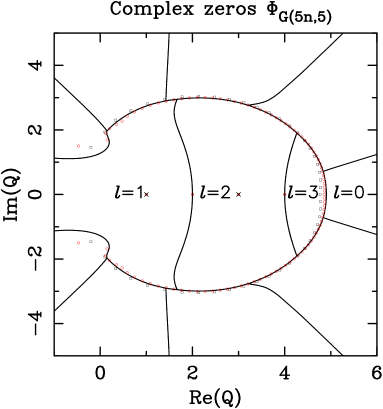
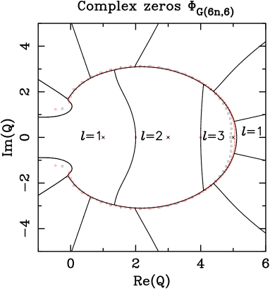
(a)	(b)
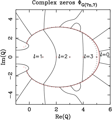
(c)

Figure 9: Complex zeros of the flow polynomial and limiting curves $\mathcal{B}_{k}$ in the complex $Q$–plane for the generalized Petersen graphs $G(nk,k)$ with $k=5$ (a), $k=6$ (b), and $k=7$ (c). The black squares ($\square$) correspond to the zeros of $G(50,5)$ (a), $G(60,6)$ (b), and $G(63,7)$ (c). The red circles ($\circ$) correspond to the zeros of $G(100,5)$ (a), $G(120,6)$ (b), and $G(119,7)$ (c). Labels are as in Figure 8.

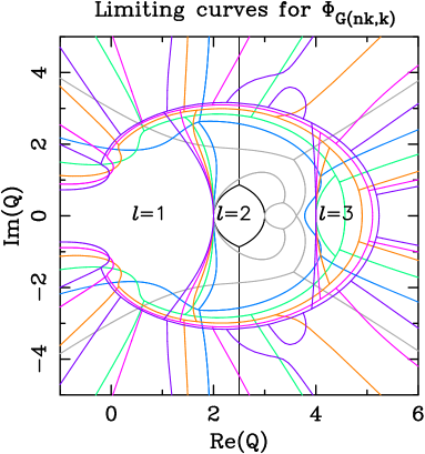
Figure 10: Limiting curves $\mathcal{B}_{k}$ for the flow polynomial in the complex $Q$-plane for the generalized Petersen graphs $G(nk,k)$ with $k=1$ (black), $k=2$ (gray), $k=3$ (light blue), $k=4$ (green), $k=5$ (orange), $k=6$ (pink), and $k=7$ (violet). Labels are as in Figure 8.

If we restrict to the cases with $k\geq 4$ (see Figures 8(d) and 9), we notice some regularities about the isolated limiting points and the dominant eigenvalues in the non-asymptotic region of the complex $Q$-plane. If we denote by $Q_{c}^{(\Phi)}$ the largest real value of $Q$ where $\mathcal{B}_{k}$ crosses the real $Q$-axis, then we conjecture that:

Conjecture 6.2

Fix $k\geq 4$. Then, the dominant eigenvalue in the regions that intersect the real $Q$-axis is

$$\mu_{\star}\;=\;\begin{cases}\;\mu_{k+1,1,(1),\star}&\;\text{for $\mathop{\rm Re}\nolimits Q\in(-\infty,2]$}\\ \;\mu_{k+1,2,(2),\star}&\;\text{for $\mathop{\rm Re}\nolimits Q\in[2,4]$}\\ \;\mu_{k+1,3,(3),\star}&\;\text{for $\mathop{\rm Re}\nolimits Q\in[4,Q_{c}^{(\Phi)}(k)]$}\\ \;\mu_{k+1,1,(1),\star}&\;\text{for $\mathop{\rm Re}\nolimits Q\in[Q_{c}^{(\Phi)}(k),\infty)$ and even $k$}\\ \;\mu_{k+1,0,\star}&\;\text{for $\mathop{\rm Re}\nolimits Q\in[Q_{c}^{(\Phi)}(k),\infty)$ and odd $k$}\end{cases}$$ (6.3)

Therefore, $Q=1$, $Q=3$ and $Q=5$ (only when $Q^{(\Phi)}_{c}(k)>5$) are isolated limiting points; and $Q=2$, $Q=4$, and $Q=Q^{(\Phi)}_{c}(k)$ are non-isolated limiting points.

Notice that the above conjecture is also valid for $k=3$, except that in this case, there is no region where the eigenvalue $\mu_{k+1,3,(3),\star}$ becomes dominant, since $Q_{c}^{(\Phi)}(3)<4$. It is worth noting that the dominant eigenvalue comes from the completely symmetric irreducible representation of $S_{\ell}$ for $\ell=1,2,3$.

Assuming that the dominant eigenvalue on the real $Q$-axis invariably comes from the completely symmetric representation, it is possible to extend the numerical determination of $Q_{c}^{(\Phi)}(k)$ to higher values of $k$. The relevant transfer matrices can be numerically diagonalized by a standard iterative scheme that uses their decomposition as a product of sparse matrices, as in (3.2). The resulting values of $Q_{c}^{(\Phi)}(k)$ are shown in Table 2.

$k$	$Q_{c}^{(\Phi)}(k)$
1	3
2	3.6180339887
3	3.7818423129
4	4.5697435537
5	4.9029018077
6	5.1079785012
7	5.2352605291
8	5.3246966903
9	5.3886186958
10	5.4364766073
11	5.4729804532

Table 2: Values of $Q_{c}^{(\Phi)}(k)$ for the generalized Petersen graphs $G(nk,k)$ for $1\leq k\leq 11$.

The values of $Q_{c}^{(\Phi)}(k)$ are seen to be well fitted by a power-law Ansatz: $Q_{c}^{(\Phi)}(k)=Q_{c}^{(\Phi)}+Ak^{-\Delta}$. To prevent possible parity effects, we performed the fits for odd and even values of $k$ separately. Both fits were consistent with each other and give a common limit $Q_{c}^{(\Phi)}=5.69(1)$. In fact, we tried a fit of the full data with an Ansatz of the form

$$Q_{c}^{(\Phi)}(k)\;=\;Q_{c}^{(\Phi)}+\begin{cases}A\,k^{-B}&\quad\text{if $k$ is even}\\ A^{\prime}\,k^{-B^{\prime}}&\quad\text{if $k$ is odd}\end{cases}$$ (6.4)

We found that 1) $Q_{c}^{(\Phi)}=5.69(1)$, 2) that the differences between $(A,B)$ and $(A^{\prime},B^{\prime})$ were very small, so the parity effects are almost eliminated by fixing a common limit for the odd and even data sub-sets, and 3) the fits were rather stable (the fits for data $5\leq k\leq 9$, $6\leq k\leq 10$, and $7\leq k\leq 11$, gave almost the same results). Finally, we also tried to extrapolate our numerical data using the Bulirsch-Stoer algorithm for the odd– and even–$k$ subsets, and for the full data set. The convergence is rather slow, and our best estimate for the limit is $Q_{c}^{(\Phi)}=5.685(10)$, which agrees with the previous estimates. We conclude that:

$$Q_{c}^{(\Phi)}\;\equiv\;\lim_{k\to\infty}Q_{c}^{(\Phi)}(k)\;=\;5.69\pm 0.01\,.$$ (6.5)

Formalizing slightly these experimental results, we conjecture that the exists a real number $Q_{c}^{(\Phi)}\approx 5.69$ that is an accumulation point of real flow zeros for the graph family $G(nk,k)$, in the limit $\lim_{n\to\infty}\lim_{k\to\infty}$, and that no generalized Petersen graph has a real flow zero above $Q_{c}^{(\Phi)}$. The hope that no graph family fares better than the generalized Petersen graph is our main motivation—and evidence—for stating Conjecture 1.9 of Ref. [30]:

Conjecture 6.3

For any bridgeless graph $G$, $\Phi_{G}(Q)>0$ for $Q\in[6,\infty)$.

This conjecture has a great interest in Combinatorics, especially in connection to Tutte’s five–flow conjecture [55, 56, 36]:

Conjecture 6.4

For any bridgeless graph $G$, $\Phi_{G}(5)>0$.

This conjecture seems at least as difficult to prove or disprove as the famous four-color conjecture (which eventually turned out to be a theorem [1]).

7 Chromatic polynomial for the generalized Petersen graphs

We have also symbolically computed the chromatic polynomial $P_{G(nk,k)}(Q)$ for the generalized Petersen graphs $G(nk,k)$ with $1\leq k\leq 6$ by specializing the full partition functions $Z_{G(nk,k)}(Q,v)$ of Sections 3 and 4 to the case $v=-1$. Again, we have checked our symbolic results against exact computations made by using Maple for the smallest values of $n\geq 1$.

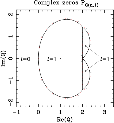
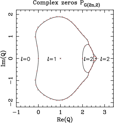
(a)	(b)
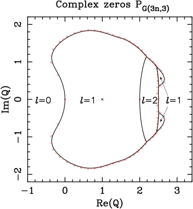
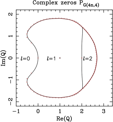
(c)	(d)

Figure 11: Complex zeros of the chromatic polynomial and limiting curves $\mathcal{B}_{k}$ in the complex $Q$–plane for the generalized Petersen graphs $G(nk,k)$ with $k=1$ (a), $k=2$ (b), $k=3$ (c), and $k=4$ (d). For each value of $k$, the zeros correspond to the generalized Petersen graphs $G(10k,k)$ (black $\square$) and $G(20k,k)$ (red $\circ$). Each region is labeled with the sector the dominant eigenvalue belongs to (e.g., $\ell=1$).

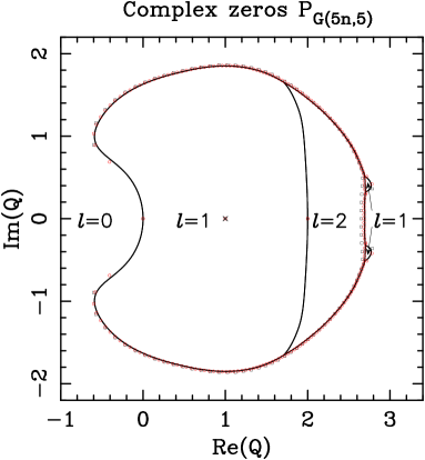
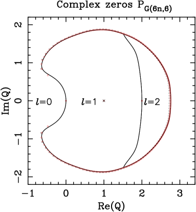
(a)	(b)
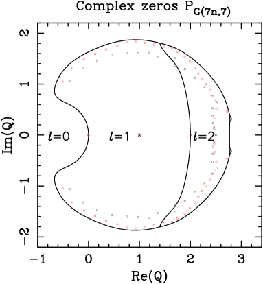
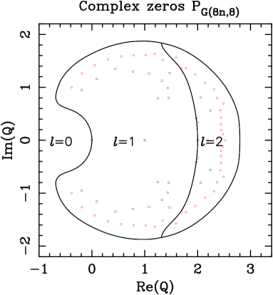
(c)	(d)

Figure 12: Complex zeros of the chromatic polynomial and limiting curves $\mathcal{B}_{k}$ in the complex $Q$–plane for the generalized Petersen graphs $G(nk,k)$ with $k=5$ (a), $k=6$ (b), $k=7$ (c), and $k=8$ (d). The black squares ($\square$) correspond to the zeros of $G(50,5)$ (a), $G(60,6)$ (b), $G(21,7)$ (c), and $G(18,8)$ (d). The red circles ($\circ$) correspond to the zeros of $G(100,5)$ (a), $G(120,6)$ (b), $G(28,7)$ (c), and $G(24,8)$ (d). The labels are as in Figure 11.

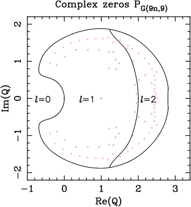
Figure 13: Complex zeros of the chromatic polynomial and limiting curves $\mathcal{B}_{k}$ in the complex $Q$–plane for the generalized Petersen graphs $G(9n,9)$. The black squares ($\square$) correspond to the zeros of $G(18,9)$, and the red circles ($\circ$) correspond to the zeros of $G(27,9)$. The labels are as in Figure 11. There are two tiny complex-conjugate oval-like regions (as for the other odd values of $k$) around $(Q,v)\approx(2.80,0.36)$; see Figure 14(b).

Again, in addition to finding the chromatic roots for finite Petersen graphs $G(nk,k)$, we are interested in their accumulation sets as $n\to\infty$. We have obtained in this way, for each value of $k$, the corresponding limiting curve $\mathcal{B}_{k}$ of non-isolated limiting points. We have used the direct search method [46] to obtain this curves with high precision arithmetic. These curves are shown in Figures 11–13. In the cases $k=7,8,9$, the chromatic zeros were obtained by using Maple. The corresponding limiting curves $\mathcal{B}_{k}$ were computed by numerically diagonalizing the relevant transfer matrices by the Arnoldi algorithm and the use of their decomposition as a product of sparse matrices, as in (3.2). This latter procedure was implemented in C.

Contrary to what happens for the flow–polynomial case, the limiting curves are bounded in the complex $Q$-plane (i.e., there are no outward branches going to infinity). This is expected because a theorem by Sokal [52, Corollary 5.3 and Proposition 5.4] states that if $G$ is a loopless finite undirected graph of maximum degree $\Delta$, then all the chromatic zeros lie in the disk $|Q|<K\Delta$, with $\Delta\approx 7.963906$. For the generalized Petersen graphs $\Delta=3$, and the bound given by this theorem is far from sharp for this family of graphs. If we restrict to the cases with $k\geq 3$ (see Figures 11(c)–(d), 12, and 13), we notice some regularities about the isolated limiting points and the dominant eigenvalues in the complex $Q$-plane. If we denote by $Q_{c}^{(P)}$ the largest real value of $Q$ where $\mathcal{B}_{k}$ crosses the real $Q$-axis, then we conjecture that:

Conjecture 7.1

Fix $k\geq 3$. Then, the dominant eigenvalue in the regions that intersect the real $Q$-axis is

$$\mu_{\star}\;=\;\begin{cases}\;\mu_{k+1,0,\star}&\;\text{for $\mathop{\rm Re}\nolimits Q\in(-\infty,0]$}\\ \;\mu_{k+1,1,(1),\star}&\;\text{for $\mathop{\rm Re}\nolimits Q\in[0,2]$}\\ \;\mu_{k+1,2,(2),\star}&\;\text{for $\mathop{\rm Re}\nolimits Q\in[2,Q_{c}^{(P)}(k)]$}\\ \;\mu_{k+1,0,\star}&\;\text{for $\mathop{\rm Re}\nolimits Q\in[Q_{c}^{(P)}(k),\infty)$}\end{cases}$$ (7.1)

Therefore, $Q=1$ is the only isolated limiting point; and $Q=0$, $Q=2$ and $Q=Q^{(P)}_{c}(k)$ are non-isolated limiting points.

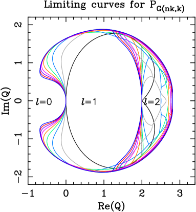
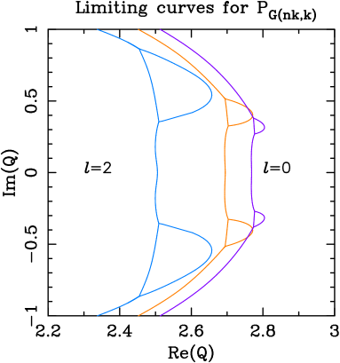
(a)	(b)

Figure 14: (a) Limiting curves $\mathcal{B}_{k}$ for the chromatic polynomial in the complex $Q$-plane for the generalized Petersen graphs $G(nk,k)$ with $k=1$ (black), $k=2$ (gray), $k=3$ (light blue), $k=4$ (green), $k=5$ (orange), $k=6$ (pink), $k=7$ (violet), $k=8$ (red), and $k=9$ (navy blue). (b) Zoom for odd values of $k=3,5,7$, where we find two small complex-conjugate closed regions. Inside them, the dominant eigenvalue comes from the $\ell=1$ sector. Notice the change of scale with respect to panel (a). We do not show the curve for $k=1$, as then the small regions for $k=7$ would be difficult to see. The labels are as in Figure 11.

$k$	$Q_{c}^{(P)}(k)$
1	2
2	2.6383423072
3	2.5054257523
4	2.6971127211
5	2.6947536196
6	2.7631358388
7	2.7682556521
8	2.7983688222
9	2.8023368562
10	2.8176338815
11	2.8203525818

Table 3: Values of $Q_{c}^{(P)}(k)$ for the generalized Petersen graphs $G(nk,k)$ for $1\leq k\leq 11$.

Note that, contrary to the flow–polynomial case, the integer $Q=0$ is a (non-isolated) limiting point. The similarities of the limiting curves can be appreciated from Figure 14(a), where we show together the limiting curves $\mathcal{B}_{k}$ for $1\leq k\leq 9$. The limiting curves seem to converge to some infinite-width curve $\mathcal{B}_{\infty}$, and the picture is qualitatively very similar to those for the square–lattice chromatic polynomial with both cyclic [28] and toroidal [29] boundary conditions. For odd values of $k$, the limiting curve $\mathcal{B}_{k}$ displays two complex-conjugate regions on its right-most part. Inside these regions, the dominant eigenvalue comes from the $\ell=1$ sector. These regions are shown for $k=3,5,7$ in Figure 14(b). It is clear that, as $k$ increases, they become smaller and closer to the real $Q$-axis. Therefore, we conjecture that they completely disappear in the limit $k\to\infty$.

Assuming that the dominant eigenvalue on the real $Q$-axis invariably comes from the completely symmetric representation, it is possible to extend the numerical determination of $Q_{c}^{(P)}(k)$ to higher values of $k$. The resulting values of $Q_{c}^{(P)}(k)$ are shown in Table 3.

The values of $Q_{c}^{(P)}(k)$ show parity effects, so we fitted the data for $k$ even and the data for $k$ odd separately. Using the same techniques as for $Q_{c}^{(\Phi)}$, we obtain in this case

$$Q_{c}^{(P)}\;\equiv\;\lim_{k\to\infty}Q_{c}^{(P)}(k)\;=\;2.861\pm 0.003\,.$$ (7.2)

The power-law fit to the odd-$k$ data gave a constant term $\approx 2.86(1)$, while for the even-$k$ data the result was $\approx 2.86(8)$. If we used the full data set with the Ansatz (6.4), we obtained $\approx 2.861$ for $7\leq k\leq 11$, and $\approx 2.864$ for $6\leq k\leq 10$. The error bar was taken as the difference between the last two estimates.

8 Discussion

In this concluding section we would like to make an unified picture of the results presented in this paper, and to propose a number of conjectures that should stimulate further research. We have seen that the $Q$-state Potts model with temperature parameter $v$ comprises both the flow polynomial ($v=-Q$), and the chromatic polynomial ($v=-1$) as special cases. It is therefore useful to compare our results on the partition function and its flow– and chromatic–polynomial specializations for the particular class of non-planar graphs $G(nk,k)$ with what is known for the same objects evaluated on certain classes of planar graphs. Our graphs are taken to consist of $n$ identical layers of width $L$ vertices and we impose periodic boundary conditions in the $n$-direction.

Before starting with the main discussion it is worth recalling the BKW theorem [11, 12, 10, 13, 53] in a simple way: Let $D$ be a domain (connected open set) $D$ in the complex plane, and let $\alpha_{1},\ldots,\alpha_{M},\mu_{1},\ldots,\mu_{M}$ ($M\geq 2$) be analytic functions on $D$, none of which is identically zero. Then, for each integer $n\geq 0$, define the functions

$$f_{n}(z)\;=\;\sum\limits_{k=1}^{M}\alpha_{k}(z)\,\mu_{k}(z)^{n}\;.$$ (8.1)

Each function $f_{n}$ has a set of complex zeros, and we are interested in the accumulation set of these zeros in the limit $n\to\infty$. Then, under a mild “no-degenerate-dominance” condition, these limiting zeros can be characterized as follows: a point $z$ lies in this limiting set if and only if either

• There is a unique dominant eigenvalue $\mu_{k}$ at $z$ (i.e., $|\mu_{k}|>|\mu_{i}|$ for all $i\neq k$), and $\alpha_{k}(z)=0$;

• There are two or more dominant eigenvalues $\mu_{k}$ at $z$.

Let us now consider first the planar chromatic case. The general situation is expected to be the following:

Conjecture 8.1

Consider a family $G_{n,L}$ of planar connected graphs, consisting of $n$ identical layers of width $L$ vertices, with periodic boundary conditions in the $n$-direction. Let $\mathcal{A}_{L}$ (resp. $\mathcal{B}_{L}$) denote the set of limiting points of chromatic zeros for $G_{n,L}$, in the limit $n\to\infty$, that satisfies condition (a) (resp. condition (b)) of the BKW Theorem. Further let $B_{p}$ be the $p$-th Beraha number (1.12), and let

$$B^{\rm even}\;=\;\left\{Q=B_{p}\,\colon\,p\in 2{\mathbb{N}}\right\}\,,\qquad B^{\rm odd}=\left\{Q=B_{p}\,\colon\,p\in 2{\mathbb{N}}+1\right\}$$

denote, respectively, the set of even and odd Beraha numbers $B_{p}$. Then:

1. There exists, for each $L$, a number $Q_{c}^{(P)}(L)\in(0,4)$ so that

   1. $\mathcal{A}_{L}\cap{\mathbb{R}}=B^{\rm odd}\cap[0,Q_{c}^{(P)}(L))$

   2. $\mathcal{B}_{L}\cap{\mathbb{R}}=B^{\rm even}\cap[0,Q_{c}^{(P)}(L))\cup\{Q_{c}^{(P)}(L)\}$

2. For any $p\in N$, the dominant eigenvalue of the transfer matrix for

   $$Q\;\in\;(B_{2p},B_{2(p+1)})\cap[0,Q_{c}^{(P)}(L))$$

   comes from the sector with $p$ marked clusters.

Compelling evidence for Conjecture 8.1 comes from the results of Ref. [28], where it was shown that Conjecture 8.1 is correct for cyclic strips of the square and triangular lattices with $L\leq 8$. The corresponding values of $Q_{c}^{(P)}(L)$ can be found in [28].

The natural step suggested by these finite-$L$ results is to go to the infinite–volume limit, $\lim_{L\to\infty}$. We expect that for each family of planar graphs $G_{n,L}$, defined as above, the limit $Q_{c}^{(P)}=\lim_{L\to\infty}Q_{c}^{(P)}(L)$ exists and satisfies $0<Q_{c}^{(P)}<4$ [49, 50, 28]. In particular for cyclic strip graphs of the square lattice, we have that $Q_{c}^{(P)}=3$ [4, 32]. For cyclic strips of the triangular lattice, we expect that either $Q_{c}^{(P)}\approx 3.8196$ [5, 6], or $Q_{c}^{(P)}=B_{12}=2+\sqrt{3}$ [31].

The deep meaning of these results is that the special role of the Beraha numbers in the production of real chromatic zeros is brought out whenever the chromatic line ($v=-1$) intersects the BK phase in the $(Q,v)$ plane of the Potts model [49, 50]. For each graph family, and for each $Q\in[0,4)$, it can be argued [33] that the extent of the BK phase is a finite non-empty interval $v_{-}(Q)<v<v_{+}(Q)$ with the properties $v_{+}(0)=0$ and $\lim_{Q\to 4}v_{+}(Q)=\lim_{Q\to 4}v_{-}(Q)$. In particular, other choices of the temperature curve $v(Q)$ are possible and might in some cases lead to higher values of $Q_{c}$ than those quoted above.

The bound on $Q_{c}$ given above is even sharp: i.e., there exists a family of planar graphs $G_{n,L}$, defined as above, and a curve $v=f(Q)$ in the $(Q,v)$ plane, so that the limiting set of zeros for the Potts-model partition function $Z_{G}(Q,v)$ satisfies Conjecture 8.1 and $Q_{c}=4$. Indeed, this is the case [49, 50, 33] for cyclic strips of the square lattice with the choice [2] $v^{2}=Q$ for $0\leq Q\leq 4$ and $-2\leq v\leq 0$. Another example is provided by cyclic strips of the triangular lattice with the choice [7] $v^{3}+3v^{2}=Q$ for $0\leq Q\leq 4$ and $-2\leq v\leq 0$.

As the amplitudes do not depend on $v$, we can extend Conjecture 8.1 to the zeros of the full partition function $Z_{G(n,L)}(Q,v)$ in the $(Q,v)$ plane:

Conjecture 8.2

Consider a family $G_{n,L}$ of planar connected graphs, consisting of $n$ identical layers of width $L$ vertices, with periodic boundary conditions in the $n$-direction. Let the sub-sets of Beraha numbers $B^{\rm even}$ and $B^{\rm odd}$ be as in Conjecture 8.1. Then:

1. There are two curves $v_{\pm}(Q)$ such that $v_{-}(Q)\leq v_{+}(Q)$, $v_{+}(0)=0$, and a number $Q_{0}\leq 4$, such that $\lim_{Q\to Q_{0}}v_{+}(Q)=\lim_{Q\to Q_{0}}v_{-}(Q)$.

Furthermore, consider any smooth curve $v(Q)$ in between these two curves: $v_{-}(Q)\leq v(Q)\leq v_{+}(Q)$ with $Q\in[0,Q_{0}]$. Let us denote its graph in the $(Q,v)$ plane as $\mathcal{C}$. Let $\mathcal{A}_{L}$ (resp. $\mathcal{B}_{L}$) denote the set of limiting points of partition-function zeros for $G_{n,L}$, in the limit $n\to\infty$, that satisfies condition (a) (resp. condition (b)) of the BKW Theorem. Then:

1. For each curve $v(Q)$ with the above properties, there exists, for each $L$, a number $Q_{c}(L)\in(0,Q_{0})$ so that

   1. $\mathop{\rm Re}\nolimits(\mathcal{A}_{L}\cap\mathcal{C})=B^{\rm odd}\cap[0,Q_{c}(L))$

   2. $\mathop{\rm Re}\nolimits(\mathcal{B}_{L}\cap\mathcal{C})=B^{\rm even}\cap[0,Q_{c}(L))\cup\{Q_{c}(L)\}$

2. For any $p\in N$, the dominant eigenvalue of the transfer matrix for

   $$\mathop{\rm Re}\nolimits Q\;\in\;(B_{2p},B_{2(p+1)})\cap[0,Q_{c}(L))\,$$

   and $\mathop{\rm Im}\nolimits Q$ in between the curves $v_{\pm}(Q)$, comes from the sector with $p$ marked clusters.

Let us finally mention that Conjectures 8.1 and 8.2 enjoys strong support from the special representation theory of the quantum group at roots of unity [49, 50].

Remark. A natural question is to determine the value of the number $Q_{0}$ defined in the previous conjecture for planar strip graphs. From the exact results for the free energy of the $Q$-state Potts antiferromagnet on the square, triangular, and hexagonal lattices [2, 7, 4, 3, 5, 6], one would be tempted to claim that $Q_{0}=4$. This value is also supported by the numerical results for the $(4,8^{2})$ and $(3,12^{2})$ lattices, obtained using the Jacobsen–Scullard method [35]. However, the same method [34, 35] suggest that $Q_{0}<4$ for the kagome lattice. Therefore, we prefer to be conservative and not make any firm conjecture about the value of $Q_{0}$ for general planar lattices.

Turning now to the partition-function zeros of non-planar graphs, Figures 3, 10, and 14, Conjectures 6.2 and 7.1, and the observations made in Section 4, makes us confident that the statements of Conjecture 8.1 hold true also in the partition-function case for non-planar graphs, provided that one replaces even/odd Beraha numbers by even/odd integers. On a fundamental level, the replacement of Beraha numbers by integers stands out most clearly by comparing the eigenvalue amplitudes in the two cases [see, e.g., [28, Eqs. (2.28)–(2.29)] and Eq. (3.4)]. To be precise:

Conjecture 8.3

Consider a family $G_{n,L}$ of non-planar connected graphs, consisting of $n$ identical layers of width $L$ vertices, with periodic boundary conditions in the $n$-direction. Then:

1. There are two curves $v_{\pm}(Q)$ such that $v_{-}(Q)\leq v_{+}(Q)$, $v_{+}(0)=0$, and there is a value $Q_{0}$ (possibly $Q_{0}=\infty$), such that $\lim_{Q\to Q_{0}}v_{+}(Q)=\lim_{Q\to Q_{0}}v_{-}(Q)$.

Furthermore, consider any smooth curve $v(Q)$ in between these two curves: $v_{-}(Q)\leq v(Q)\leq v_{+}(Q)$ with $Q\in[0,Q_{0}]$. Let us denote its graph in the $(Q,v)$ plane as $\mathcal{C}$. Let $\mathcal{A}_{L}$ (resp. $\mathcal{B}_{L}$) denote the set of limiting points of partition-function zeros for $G_{n,L}$, in the limit $n\to\infty$, that satisfies condition (a) (resp. condition (b)) of the BKW Theorem. Then:

1. For each curve $v(Q)$ with the above properties, there exists, for each $L$, a number $Q_{c}(L)\in(0,Q_{0})$ so that

   1. $\mathop{\rm Re}\nolimits(\mathcal{A}_{L}\cap\mathcal{C})=(2{\mathbb{N}}-1)\cap[0,Q_{c}(L))$

   2. $\mathop{\rm Re}\nolimits(\mathcal{B}_{L}\cap\mathcal{C})=2{\mathbb{N}}\cap[0,Q_{c}(L))\cup\{Q_{c}(L)\}$. For some curves $v(Q)$ the value $0$ might not be present in this set.

2. For any $p\in N$, the dominant eigenvalue of the transfer matrix for

   $$\mathop{\rm Re}\nolimits Q\;\in\;(2(p-1),2p)\cap[0,Q_{c}(L))\,$$

   and $\mathop{\rm Im}\nolimits Q$ in between the curves $v_{\pm}(Q)$, comes from the fully symmetric irreducible representation $(p)$ of the sector with $p$ marked clusters.

This conjecture has been validated in this paper for $G_{n,L}=G(nk,k)$, the generalized Petersen graphs, with $L=k+1$, and $k\leq 7$ for the flow polynomial $v(Q)=-Q$, and the chromatic polynomial $v(Q)=-1$. We have also presented numerical evidence that the limits $Q_{c}$ exist along these two curves $v(Q)$. In addition, we have directly checked the consistency of this picture (at least for $k\leq 7$) by considering directly the partition-function zeros along several lines $v(Q)=-pQ$, $v(Q)=-Q/p$, and $v(Q)=-p$ with $p$ a positive integer (see Section 4).

Remark. The set $\mathop{\rm Re}\nolimits(\mathcal{B}_{L}\cap\mathcal{C})$ does not contain the value $0$ for the flow polynomial; but it contains this value for the chromatic-polynomial case. The difference might be due to the fact that when $Q<0$ we enter in the ferromagnetic regime in the former case, while we stay in the antiferromagnetic or unphysical regime in the latter case.

To conclude, we recall that for the Potts model on planar graphs $G_{n,L}$, when $Q=\big{(}2\cos(\pi/p)\big{)}^{2}$ is a Beraha number the representation theory of the underlying quantum algebra [39] leads to massive degeneracies in the spectrum of the transfer matrix. In particular, depending on $p$, complete sectors of eigenvalues are contained in other sectors in an inclusion-exclusion fashion, completely independent of the value of $v$. We have seen in Section 5 that a similar phenomenon occurs for the Potts model on non-planar graphs when $Q$ is a non-negative integer. There are striking parallels between the detailed inclusion-exclusion scenarios in the two cases, once again provided that one “translates” between the two cases by replacing the Beraha numbers by non-negative integers.

Appendix A Potts–model partition function for the simple-cubic graphs

A natural question is that our conclusions are based on a rather particular family of non-planar graphs. In this appendix we want to examine a more “physical” family of graphs: the graphs $\text{Sc}(L,n)$ formed by a simple cubic graph of section of size $L\times L\times n$ with cyclic boundary conditions (i.e., free boundary conditions in the transverse “space-like” two–dimensional layers, and periodic boundary conditions in the longitudinal “time-like” direction). The chromatic polynomial for this family was previously considered in Ref. [45].

The graph $\text{Sc}(L,n)$ contains $L^{2}n$ vertices, $2(L-1)Ln$ horizontal edges, and $L^{2}n$ vertical edges. If we denote the vertices in $\text{Sc}(L,n)$ as points in ${\mathbb{Z}}_{+}^{3}$, the vertex set is

$$V(\text{Sc}(L,n))\;=\;\{(x,y,z)\mid 0\leq x,y\leq L-1\,,\;0\leq z\leq n-1\}\,,$$ (A.1)

and the edge set is the union of the sets $E(\text{Sc}(L,n))=E_{x}\cup E_{y}\cup E_{z}$, where

$$E_{x}&=\{((x,y,z),(x+1,y,z))\mid 0\leq x\leq L-2\,,\,0\leq y\leq L-1\,,\;0\leq z\leq n-1\}\quad\\ E_{y}=\{((x,y,z),(x,y+1,z))\mid 0\leq x\leq L-1\,,\,0\leq y\leq L-2\,,\;0\leq z\leq n-1\}\quad\\ E_{z}=\{((x,y,z),(x,y,z+1))\mid 0\leq x,y\leq L-1\,,\;0\leq z\leq n-1\}$$ (A.2)

where we have identified $z=n$ and $z=0$.

We can apply the transfer-matrix formalism of Section 3 to the family $\text{Sc}(L,n)$. If we label the vertices on a horizontal layer as $(x,y)$ with $0\leq x,y\leq L-1$, then the transfer matrix takes the form ${\sf T}_{L}={\sf V}\cdot{\sf H}$ with

$${\sf H}&=\prod\limits_{y=0}^{L-1}\prod_{x=0}^{L-2}{\sf H}_{(x,y),(x+1,y)}\cdot\prod\limits_{x=0}^{L-1}\prod_{y=0}^{L-2}{\sf H}_{(x,y),(x,y+1)}\\ {\sf V}=\prod\limits_{y=0}^{L-1}\prod_{x=0}^{L-1}{\sf V}_{(x,y)}$$ (A.3)

The order of the operators ${\sf H}_{(x,y),(x+1,y)}$ and ${\sf H}_{(x,y),(x,y+1)}$ in (A.3a) is of no importance, as all the horizontal operators commute. The same also holds for the vertical operators ${\sf V}_{(x,y)}$ in (A.3b). However, the operators ${\sf H}$ and ${\sf V}$ do not commute.

The computation of the partition function for the graph $\text{Sc}(L,n)$ is quite demanding: the number of partitions we have to deal with is given by the Bell number $B_{2L^{2}}$ [30, and references therein]. This number grows very fast as a function of $L$. The formula for the partition function for $G=\text{Sc}(L,n)$ is given in terms of traces of the relevant diagonal blocks of the full transfer matrix ${\sf T}_{L}$:

$$Z_{\text{Sc}(L,n)}(Q,v)\;=\;\sum\limits_{\ell=0}^{L^{2}}\sum\limits_{\lambda\in S_{\ell}}\alpha_{\ell,\lambda}\,\mathop{\rm tr}\nolimits\left({\sf T}_{L,\ell,\lambda}\right)^{n}\,.$$ (A.4)

Some of the eigenvalues of the transfer matrices ${\sf T}_{L,\ell,\lambda}$ may coincide.

In practice, we have been able to compute only the exact partition function for $L=2$. The structural properties of the transfer matrix ${\sf T}_{2}$ can be summarized as follows:

• The trivial eigenvalue $\mu_{2,4}=v^{4}$ appears for all values of the number of links $0\leq\ell\leq L^{2}=4$ with multiplicities $2,6,12,24$. This implies that the corresponding amplitude is $\gamma_{4}=Q^{2}-8Q^{3}+20Q^{2}-15Q+1$.

• For $\ell=0$ there are two eigenvalues that appear twice; therefore in the “complete” representation of $Z_{\text{Sc}(2,n)}$, they should have the amplitude $2\alpha_{0}=2$.

• For $\ell=1$, there are eight eigenvalues that appear twice; therefore their amplitude is $2\alpha_{1}=2(Q-1)$.

• For $\ell=2$, there are four eigenvalues that appear twice in both representations $(2)$, and $(1,1)$. Its amplitude is $\alpha_{2,(2)}+\alpha_{2,(1,1)}=2(Q^{2}-3Q+1)$. In addition, there are six eigenvalues in the representation $(2)$ that appear twice; and another six eigenvalues in $(1,1)$ that appear twice, too. Their corresponding amplitude should be twice the value $\alpha_{1,\lambda}$.

• For $\ell=3$, the representations $(3)$ and $(1,1,1)$ have exactly the same eigenvalues. Their amplitude is $(Q-1)(Q^{2}-5Q+3)/3$. Two of these eigenvalues appear twice in each representation, therefore their amplitude is twice the latter value. The representation $(2,1)$ has all its eigenvalues doubled; hence their amplitude is $2Q(Q-2)(Q-4)/3$.

The number of non-trivial distinct eigenvalues in each $\ell$ sector are $12,27,39,14$ for $\ell=0,1,2,3$, respectively. We then obtain a “complete” decomposition of $Z_{\text{Sc}(2,n)}$ in terms of distinct eigenvalues $\mu_{L,\ell,\lambda,s}$. The full expression is rather cumbersome, so we refrain from writing it explicitly here.

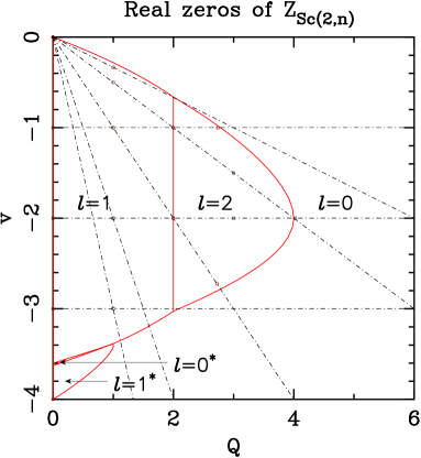
Figure 15: Real zeros of the Potts-model partition function and limiting curves $\mathcal{B}_{2}$ in the plane $(Q,v)$ for the simple-cubic graphs $\text{Sc}(2,n)$ for $n=9$ (black $\square$), and $n=10$ (red $\circ$). The rest of the notation is as in Figure 1.

We have computed the zeros of the partition function $Z_{\text{Sc}(2,n)}(Q,v)$ along the same lines in the real $(Q,v)$ plane as for the generalized Petersen graphs. Figure 15 shows these zeros for the simple–cubic graphs $\text{Sc}(2,9)$ and $\text{Sc}(2,10)$.

We have also computed the limiting curve $\mathcal{B}_{2}$ in the real $(Q,v)$ plane; this is depicted in Figure 15. The phase structure for this family of graphs is similar to that described for the generalized Petersen graphs. In particular, we can observe two phases enclosed by the limiting curve $\mathcal{B}_{2}$ and characterized by $\ell=1$ and $\ell=2$ respectively. The former contains the interval $Q\in(0,2)$, and the latter, the interval $Q\in(2,4)$. In each phase, the dominant eigenvalue comes from the fully symmetric representation of the corresponding group $S_{\ell}$. Therefore, as the expressions for these eigenvalues are the same as for the generalized Petersen graphs, the values $Q=1$ and $Q=3$ are isolated limiting curves. Notice that there is no isolated limiting point at $Q=B_{5}$.

Finally, we observe close to the lower boundary of the BK phase, two regions with dominant pairs of complex-conjugate eigenvalues. This feature was absent in the Petersen graphs.

In conclusion, we find a phase diagram for this family of non-planar graphs which is qualitatively similar to that of the Petersen graphs. This supports our belief that the results we have found for the Petersen graphs are general for at least all families of recursive non-planar graphs.

References

- [1] K.I. Appel and W. Haken, Illinois J. Math. 21, 429–567 (1977).
- [2] R.J. Baxter, J. Phys. C: Solid State Phys. 6, L445–L448 (1973).
- [3] R.J. Baxter, Exactly Solved Models in Statistical Mechanics (Academic Press, London–New York, 1982).
- [4] R.J. Baxter, Proc. Roy. Soc. London A 383, 43–54 (1982).
- [5] R.J. Baxter, J. Phys. A: Math. Gen. 19, 2821–2839 (1986).
- [6] R.J. Baxter, J. Phys. A: Math. Gen. 20, 5241-5261 (1987).
- [7] R.J. Baxter, H.N.V. Temperley and S.E. Ashley, Proc. Roy. Soc. London A 358, 535–559 (1978).
- [8] A. Bedini and J.L. Jacobsen, J. Phys. A: Math. Theor. 43, 385001 (2010), arXiv:1003.4847.
- [9] S. Beraha, Infinite non-trivial families of maps and chromials. PhD Thesis, John Hopkins University, 1975.
- [10] S. Beraha and J. Kahane, J. Combin. Theory Ser. B 27, 1–12 (1979).
- [11] S. Beraha, J. Kahane and N.J. Weiss, Proc. Nat. Acad. Sci. USA 72, 4209 (1975).
- [12] S. Beraha, J. Kahane and N.J. Weiss, Limits of zeroes of recursively defined families of polynomials, in Studies in Foundations and Combinatorics (Advances in Mathematics Supplementary Studies, Vol. 1), ed. G.-C. Rota, pp. 213–232 (Academic Press, New York, 1978).
- [13] S. Beraha, J. Kahane and N.J. Weiss, J. Combin. Theory Ser. B 28, 52–65 (1980).
- [14] D.A. Bini and G. Fiorentino, Numerical computation of polynomial roots using MPSolve version 2.2 (January 2000). Software package and documentation available for download at ftp://ftp.dm.unipi.it/pub/mpsolve/MPSolve-2.2.tgz
- [15] D.A. Bini and G. Fiorentino, Num. Algorithms 23, 127–173 (2000).
- [16] G.D. Birkhoff and D.C. Lewis, Trans. Amer. Math. Soc. 60, 355–451 (1946).
- [17] S.-C. Chang, J.L. Jacobsen, J. Salas and R. Shrock, J. Stat. Phys. 114, 763–823 (2004), arXiv:cond-mat/0211623.
- [18] S.-C. Chang, J. Salas and R. Shrock, J. Stat. Phys. 107, 1207–1253 (2002), arXiv:cond-mat/0108144.
- [19] S.-C. Chang and R. Shrock, Physica A296, 131–182 (2001), arXiv:cond-mat/0005232.
- [20] S.-C. Chang and R. Shrock, J. Stat. Phys. 112 815–879 (2003), arXiv:cond-mat/0205424.
- [21] S. Dasmahapatra and P. Martin, J. Phys. A: Math. Gen. 29, 263 (1996).
- [22] C.M. Fortuin and P.W. Kasteleyn, Physica 57, 536–564 (1972).
- [23] A. Guttmann and I.G. Enting, J. Phys. A 27, 5801-5812 (1994), arXiv:hep-lat/9312083.
- [24] T. Halverson and A. Ram, Eur. J. Comb. 26, 869–921 (2005), arXiv:math/0401314.
- [25] B. Jackson, J. Geom. 76, 95–109 (2003), arXiv:math/0205047.
- [26] J.L. Jacobsen, J.–F. Richard, and J. Salas, Nucl. Phys. B 743, 153–206 (2006), arXiv:cond-mat/0511059.
- [27] J.L. Jacobsen and J. Salas, J. Stat. Phys. 104, 701–723 (2001), arXiv:cond-mat/0011456.
- [28] J.L. Jacobsen and J. Salas, J. Stat. Phys. 122, 705–760 (2006), arXiv:cond-mat/0407444.
- [29] J.L. Jacobsen and J. Salas, Nucl. Phys. B 783, 238–296 (2007), arXiv:cond-mat/0703228.
- [30] J.L. Jacobsen and J. Salas, J. Combin. Theory B 103, 532–565 (2013), arXiv:1009.4062.
- [31] J.L. Jacobsen, J. Salas and A.D. Sokal, J. Stat. Phys. 112, 921–1017 (2003), arXiv:cond-mat/0204587.
- [32] J.L. Jacobsen and H. Saleur, Nucl. Phys. B 743, 207–248 (2006), arXiv:cond-mat/0512058.
- [33] J.L. Jacobsen and H. Saleur, J. Stat. Phys. 132, 707–719 (2008), arXiv:0803.2665.
- [34] J.L. Jacobsen and C.R. Scullard, J. Phys. A: Math. Theor. 45, 494003 (2012); arXiv:1205.0622.
- [35] J.L. Jacobsen and C.R. Scullard, J. Phys. A: Math. Theor. 46, 075001 (2013); arXiv:1211.4335.
- [36] F. Jaeger, Nowhere-zero flow problems, in L.W. Beineke and R.J. Wilson (eds.), Selected topics in graph theory 3 (Academic Press, 1988).
- [37] W. Janke and R. Villanova, Nucl. Phys. B 489, 679–696 (1997), arXiv:hep-lat/9612008.
- [38] J. Oxley and D. Welsh, Combin. Probab. Comput. 11, 403 (2002).
- [39] V. Pasquier and H. Saleur, Nucl. Phys. B 330, 523–556 (1990).
- [40] V. Pasquier and H. Saleur, Nucl. Phys. B 330, 523–556 (1990).
- [41] R.B. Potts, Proc. Camb. Phil. Soc. 48, 106–109 (1952).
- [42] N. Read and H. Saleur, Nucl. Phys. B 613, 409 (2001), arXiv:hep-th/0106124.
- [43] J.-F. Richard and J.L. Jacobsen, Nucl. Phys. B 750, 250–264 (2006), arXiv:math-ph/0605016.
- [44] J.-F. Richard and J.L. Jacobsen, Nucl. Phys. B 769, 256–274 (2007), arXiv:math-ph/0608055.
- [45] J. Salas and R. Shrock, Phys. Rev. E 64, 0111111 (2001), arXiv:cond-mat/0102190.
- [46] J. Salas and A.D. Sokal, J. Stat. Phys. 104, 609-699 (2001), arXiv:cond-mat/0004330.
- [47] J. Salas and A.D. Sokal, J. Stat. Phys. 135, 279-373 (2009), arXiv:0711.1738.
- [48] J. Salas and A.D. Sokal, J. Stat. Phys. 144, 1028-1122 (2011), arXiv:1002.3761.
- [49] H. Saleur, Comm. Math. Phys. 132, 657–679 (1990).
- [50] H. Saleur, Nucl. Phys. B 360, 219–263 (1991).
- [51] R. Shrock, Discrete Math. 231, 421–446 (2001), arXiv:cond-mat/9908387.
- [52] A.D. Sokal, Comb. Prob. Comp. 10, 41–77 (2001), arXiv:cond-mat/9904146.
- [53] A.D. Sokal, Comb. Prob. Comp. 13, 221–261 (2004), arXiv:cond-mat/0012369.
- [54] W.T. Tutte, Proc. London Math. Soc. 51, 474–483 (1950).
- [55] W.T. Tutte, Can. J. Math. 6, 81–90 (1954).
- [56] W.T. Tutte, Graph theory (Addison-Wesley, New York, 1984).
- [57] M.E. Watkins, J. Combin. Theory 6, 152–164 (1969).
- [58] F.Y. Wu, Rev. Mod. Phys. 54, 235–268 (1982) 235; errata Rev. Mod. Phys. 55, 315 (1983).
- [59] F.Y. Wu and Y.K. Wang, J. Math. Phys. 17, 439 (1976).
- [60] C.-Q. Zhang, Integer flows and cycle covers of graphs (Marcel Dekker, New York, 1997).