Density of one-particle states for 2D electron gas in magnetic field

Abstract

The density of states of a particle in a 2D area is independent both of the energy and form of the area only at the region of large values of energy. If energy is small, the density of states in the rectangular potential well essentially depends on the form of the area. If the bottom of the potential well has a potential relief, it can define the small eigenvalues as the discrete levels. In this case, dimensions and form of the area would not have any importance. If the conservation of zero value of the angular momentum is taken into account, the effective one-particle Hamiltonian for the 2D electron gas in the magnetic field in the circle is the Hamiltonian with the parabolic potential and the reflecting bounds. It is supposed that in the square, the Hamiltonian has the same view. The 2D density of states in the square can be computed as the convolution of 1D densities. The density of one-particle states for 2D electron gas in the magnetic field is obtained. It consists of three regions. There is a discrete spectrum at the smallest energy. In the intervening region the density of states is the sum of the piecewise continuous function and the density of the discrete spectrum. At great energies, the density of states is a continuous function. The Fermi energy dependence on the magnetic field is obtained when the field is small and the Fermi energy is located in the region of continuous spectrum. The Fermi energy has the oscillating correction and in the average it increases proportionally to the square of the magnetic induction. Total energy of electron gas in magnetic field also oscillates and increases when the magnetic field increases monotonously.

Key words: density of states, electron gas, magnetic field, energy spectrum, Fermi energy, total energy

PACS: 05.30.Ch, 75.20.-g

Abstract

Густина станiв частинки у 2D областi не залежить вiд енергiї i форми областi тiльки при великих значеннях енергiї. При малiй енергiї густина станiв у прямокутнiй потенцiальнiй ямi суттєво залежить вiд форми областi. Якщо дно потенцiальної ями має потенцiальний рельєф, то вiн може визначати малi власнi значення енергiї як дискретнi рiвнi. У цьому випадку розмiри i форма областi не мають значення. Якщо приймати до уваги збереження нульового значення кутового моменту, ефективний одночастинковий Гамiльтонiан для 2D електронного газу у магнiтному полi у колi є Гамiльтонiаном з параболiчним потенцiалом i вiдбиваючими границями. Припускається, що у квадратi Гамiльтонiан має такий самий вигляд. 2D густина станiв у квадратi може бути обчислена як згортка 1D густин. Обчислено густину станiв 2D електронного газу у магнiтному полi. Вона складається з трьох областей. Коли енергiї малi, спектр є дискретним. У промiжнiй областi густина станiв є сумою промiжково-неперервної функцiї i густини дискретного спектру. При великих значеннях енергiї густина станiв є неперервною функцiєю енергiї. Одержано залежнiсть енергiї Фермi вiд магнiтного поля, коли поле є слабким i енергiя Фермi знаходиться в областi неперервного спектру. Енергiя Фермi має доданок, який осцилює i, в серед+ньому, зростає пропорцiйно квадрату магнiтної iндукцiї. Повна енергiя електронного газу у магнiтному полi також осцилює i зростає, коли магнiтне поле монотонно збiльшується.

Ключовi слова: густина станiв, електронний газ, магнiтне поле, енергетичний спектр, енергiя Фермi, повна енергiя

1 Introduction

The spectrum of one-particle Hamiltonian in a bounded area is discrete. When values of energy are more than maximum of potential energy (in the fourth section this criterion will be improved), the distances between levels are of the order $\hbar^{2}/2mW^{2/D}$. Here, $m$ is the mass of the particle, $W$ is the volume of the area, and $D$ is the dimensionality of space. When the volume of the area is macroscopic, the spectrum may be considered as quasicontinuous.Then, the density of states $\mathfrak{N}_{D}(E)$ may be introduced:

$$\mathfrak{N}_{D}(E)=\frac{N_{D}(E+\delta E)-N_{D}(E)}{\delta E}\,.$$ (1)

Here, $N_{D}(E)$ is the number of states, energy eigenvalues of which are less than $E$, $\delta E$ is a small interval of energy which is larger than the distances between discrete levels. Function $N_{D}(E)$ was considered mathematically rigorously in the monograph [1]. The Schrödinger equation was multiplied by $2m/\hbar^{2}$, and the eigenvalue $\varepsilon=2mE/\hbar^{2}$ has the dimension of physical quantity $[L^{-2}]$ (for brevity let us also refer to it as ‘‘energy’’). It was shown that the asymptotical formulae at $\varepsilon\to\infty$ for functions $N_{D}(\varepsilon)$ are:

$$N_{2}(\varepsilon)<\frac{S}{4\pi}\varepsilon+\theta c\sqrt{\varepsilon},\qquad N_{3}(\varepsilon)<\frac{V}{6\pi^{2}}\varepsilon^{3/2}+\theta c\varepsilon,$$ (2)

when the wave functions are equal to zero at the boundaries of the area. Here, $|\theta|<1$ and $c$ is independent of $\varepsilon$. It is important that the first terms of these formulae are independent of the form of the area. The functions $N_{D}(\varepsilon)$ take only integer values. If this is neglected when energy is great, the formula (1) can be considered as $\mathfrak{N}_{D}=\partial N_{D}/\partial\varepsilon$. Then, we can obtain from the formulae (2):

$$\mathfrak{N}_{2}=\frac{S}{4\pi}\,,\qquad\mathfrak{N}_{3}=\frac{V}{4\pi^{2}}\sqrt{\varepsilon},$$ (3)

if only the first terms of the asymptotical expansions are taken into account. Evidently, extrapolation of the formulae (3) to small values of energy is incorrect even when there is no potential energy.

In the second section of this work, the density of states at small energy is considered in the absence of a potential energy.

In the third section of this work the 2D density of states is considered in the potential well that is created by the harmonic potential and the reflecting boundaries. As is shown in the work [2], this potential takes place in the effective one-particle Hamiltonian of the electron gas in the magnetic field. The dependencies on the magnetic field are investigated for the Fermi energy and for the total energy of the gas.

The fourth section is a mathematical supplement. The problem on the linear harmonic oscillator with condition zeroes of wave function at the segment ends is considered.

2 The density of states in a square

The derivation of the formula (2) for $N_{2}(\varepsilon)$ starts from consideration of the square with $S=L^{2}$ (see monograph [1]). The states are determined by two integer numbers. The energy of state $|kl\rangle$ is $\varepsilon_{kl}=\pi^{2}(k^{2}+l^{2})/L^{2}$. Then, $N_{2}(\varepsilon)$ will be equal to the number of junctions of the net of squares that are parallel to the coordinate axes and have the sides equal to unit, which fit into the interior of the positive quadrant of the circle with radius $(L/\pi)\sqrt{\varepsilon}$. This quantity differs from the area of the quadrant $S\varepsilon/4\pi$ by the sum of areas of partial squares that are crossed by the circle. The second term in the formula (2) is the approximate estimate of this amendment. The relative magnitude of this amendment will be smaller, when the quadrant radius is larger.

Let us consider the other method of calculating the state density in the quadratic area that can be used for small energy values too. The 2D Schrödinger equation for a free particle, provided that the wave function is equal zero at the boundaries of the square, can be changed by two identical 1D equations. An eigenvalue of the 2D equation is the sum of eigenvalues of 1D equations. Therefore, let us consider the state density for the 1D equation.

The number of states, whose eigenvalues are less than $\varepsilon$ for 1D equation, is as follows: $N_{1}(\varepsilon)=\lceil L\sqrt{\varepsilon}/\pi\rceil$. Here, $\lceil\alpha\rceil$ denotes the integer part of the number $\alpha$. The density of states that is determined by formula (1) is an interval function rather than a point function. The magnitude of the interval cannot be taken arbitrarily small. In 1D, this magnitude is limited by the demand that one eigenvalue should be in the interval at the greatest energy $\varepsilon_{\mathrm{m}}$. Then,

$$\frac{L}{\pi}\left(\sqrt{\varepsilon_{\mathrm{m}}+\delta}-\sqrt{\varepsilon_{\mathrm{m}}}\right)\geqslant 1,\qquad\delta\geqslant\left(\frac{\pi}{L}\right)^{2}+\frac{2\pi}{L}\sqrt{\varepsilon_{\mathrm{m}}}\approx\frac{2\pi}{L}\sqrt{\varepsilon_{\mathrm{m}}}\,.$$ (4)

In most cases, the density of states is used in integral formulae. Then, an interval function can be changed by a piecewise continuous stepped function or a continuous differentiable function that is determined by any method of interpolation. It is apparent that the consideration of peculiarities of the state density is meaningless.

Let us determine the state density for the square at the values of energy that are smaller than $\varepsilon_{\mathrm{m}}$. The interval $\delta$ is determined by the formula (4), and it is accepted as the unity of energy. Non-dimensional ($\varepsilon/\delta$) eigenvalues of energy for 1D equation are denoted as $\lambda_{1}$ and $\lambda_{2}$, and non-dimensional eigenvalue of energy for 2D equation is denoted as $\mu,\;\mu=\lambda_{1}+\lambda_{2}$. Let us consider the intervals $[\lambda_{1},\lambda_{1}+1]$ and $[\lambda_{2}-1,\lambda_{2}]$ where $\lambda_{2}=\mu-\lambda_{1}$. The eigenfunctions of the 2D equation that are products  of  the  eigenfunctions 1D equations, which are related to these intervals, have the eigenvalues that are located at interval $[\mu-1,\mu+1]$. The number of these states is denoted as $M_{2}(\mu-1,\mu+1)$. In a similar way, the eigenvalues of the 2D equation that are located at the interval $[\mu,\mu+2]$ are obtained when $\lambda_{2}=\mu-\lambda_{1}+1$. Then, the number of the eigenvalues of the 2D equation at the interval $[\mu,\mu+1]$ (when $\mu\geqslant 2$) is:

$$M_{2}(\mu,\mu+1) = \frac{1}{2}\sum_{\lambda=0}^{\mu-1}M_{1}(\lambda,\lambda+1)M_{1}(\mu-\lambda-1,\mu-\lambda)$$ (5)

$${}+\frac{1}{2}\sum_{\lambda=0}^{\mu}M_{1}(\lambda,\lambda+1)M_{1}(\mu-\lambda,\mu-\lambda+1).$$

It follows from the formula (4) that:

$$M_{1}(\lambda,\lambda+1)=\frac{L\sqrt{\delta}}{\pi}\left(\sqrt{\lambda+1}-\sqrt{\lambda}\right).$$ (6)

Then, $M_{2}(\mu,\mu+1)=(L^{2}\delta/2\pi^{2})\varSigma(\mu)$, where

$$\varSigma(\mu) = -\sum_{i=1}^{\mu-1}\left(\sqrt{i}\right)\left(\sqrt{\mu-i+1}-\sqrt{\mu-i-1}\right)$$ (7)

$${}+\sum_{i=0}^{\mu-1}\left(\sqrt{i+1}\right)\left(\sqrt{\mu-i+1}-\sqrt{\mu-i-1}\right)+\sqrt{\mu+1}-\sqrt{\mu}.$$

This function of integer argument can be written as:

$$\varSigma(\mu)=S(\mu+1)-S(\mu)-S(\mu-1)+S(\mu-2),$$ (8)

where

$$S(x)=\sum_{n=0}^{x-1}\sqrt{(n+1)(x-n)},\qquad x\geqslant 1;\qquad S(0)=0.$$ (9)

The function $S(x)$ can be computed using Euler-Maclaurin method:

$$S(x)=\left(\frac{x+1}{2}\right)^{2}\arcsin{\frac{x-1}{x+1}}+x\sqrt{x}-\frac{x-1}{12\sqrt{x}}\,.$$ (10)

Based on the approximate formula

$$\arcsin{\frac{x-1}{x+1}}=\frac{\pi}{2}-\frac{2}{\sqrt{x+1}}-\frac{1}{3(x+1)^{3/2}}+\frac{9}{4(x+1)^{5/2}}\,,$$ (11)

the asymptotical formula

$$\varSigma(\mu)\approx\frac{\pi}{2}+\frac{3}{4\sqrt{\mu}}$$ (12)

can be obtained. The function $\varSigma(\mu)$ can be calculated numerically. The results are obtained from the formula (7) and from the asymptotical formula (12) tabulated in table 1. The values of the function $\varSigma(\mu)$ approach $\pi/2=1.57096$ from above.

Table 1: The function $\Sigma(\mu)$ that is numerically calculated [formula (7)], and calculated using an asymptotical formula (12).

$\mu$	1	10	100	1000	10,000	100,000	1,000,000
formula (7)	1.81	1.577	1.571	1.5708	1.570797	1.570796
formula (12)			1.65	1.59	1.578	1.573	1.5715

For sufficiently large value $\mu$ the density of states in a square is described by formula:

$$\mathfrak{N}_{2}(\varepsilon=\mu\delta)=\frac{M_{2}(\mu,\mu+1)}{\delta}=\frac{L^{2}}{2\pi^{2}}\varSigma(\mu)\approx\frac{L^{2}}{4\pi}+\frac{3L^{2}\sqrt{\delta}}{8\pi^{2}\sqrt{\varepsilon}}\,.$$ (13)

The first term in this formula coincides with the common expression for 2D system. It can be obtained by differentiation $N_{2}(\varepsilon)$ [formula (2)], where $S=L^{2}$. This formula can be used for derivation of the density of states for a flat geometrical figure of arbitrary shape (see monograph [1]). In this process, $L^{2}$ is changed by the figure area $S$ and amendments are proportional to $\varepsilon^{-1/2}$, i.e., they alter the second term in the formula (13). Therefore, the second term depends on the figure shape and on the interval magnitude $\delta$.

The sign of the second term also depends on the figure shape. In the square this term is positive, i.e., when the energy increases, the density of states decreases tending to the constant value from above. This is explained by the fact that in 1D, the state density increases when the energy decreases. The eigenfunctions in a circle are the Bessel functions of the first kind $J_{n}(r\sqrt{\varepsilon})$. The eigenvalues in this case are $\varepsilon_{nk}=j_{nk}^{2}/R^{2}$ where $R$ is the circle radius, and $j_{nk}$ is the null of the function $J_{n}$ that has the number $k$ in the order of increasing. There is no formula that describes these nulls when their numbers $k$ are small, but it is known that the distances between nulls increase when their numbers decrease. Therefore, the density of states should decrease when the energy decreases, and the amendment should be negative.

In fact the spectrum at small energy values is formed by the potential relief of the bottom of the potential well. The distances between energy levels are determined by parameters of this relief. Therefore, this spectrum cannot be considered as quasicontinuous. The density of states in this case can be described by the set of $\delta$-functions. By virtue of the fact that the determining factor is the potential relief, it is believed that the figure shape is of no significance. Then, it may be helpful to obtain the state density for the square in the whole region of energy values.

If the 2D Schrödinger equation with the potential energy can be solved by separating the variables in the Cartesian coordinates, then the 2D density of states can be obtained. Every interval $[\varepsilon_{1},\varepsilon_{1}+\mathrm{d}\varepsilon]$ on the axis of energy of 1D states contains $\mathfrak{N}_{1}(\varepsilon_{1})\mathrm{d}\varepsilon$ states, whose wave functions are $\psi(x_{1})$. Products of these functions with the wave functions $\psi(x_{2})$ that have the energy values in the interval $[\varepsilon_{2},\varepsilon_{2}+\mathrm{d}\varepsilon]$, where $\varepsilon_{2}=\varepsilon-\varepsilon_{1}$, are the wave functions of the 2D states, the energies of which are in the interval $[\varepsilon,\varepsilon+\mathrm{d}\varepsilon]$. The number of these states connected with the energy value $\varepsilon_{1}$ is:

$$\mathrm{d}M_{2}(\varepsilon,\varepsilon_{1})=\mathfrak{N}_{1}(\varepsilon_{1})\mathfrak{N}_{1}(\varepsilon-\varepsilon_{1})\mathrm{d}\varepsilon\mathrm{d}\varepsilon.$$ (14)

Then, the density of states in the square is:

$$\mathfrak{N}_{2}(\varepsilon)=\frac{\mathrm{d}M_{2}(\varepsilon)}{\mathrm{d}\varepsilon}=\int_{0}^{\varepsilon}\mathfrak{N}_{1}(\alpha)\mathfrak{N}_{1}(\varepsilon-\alpha)\mathrm{d}\alpha,$$ (15)

i.e., it is a convolution of 1D densities of states.

The form of the spectrum in the region of small energy values can play a significant role depending on the form of the potential relief of quantities that are determined by integral formulae.

3 The density of states and energy of 2D electron gas in the magnetic field

It is shown in the work [2] that the statistical operator of the electron gas in the magnetic field is defined by effective Hamiltonian that is the sum of the same one-particle Hamiltonians. Each one-particle Hamiltonian describes the particle in the potential well with a harmonic potential and reflecting boundaries. Electrons interact with each other and with the neutralizing background. The electron density in the magnetic field should be distributed in such a way as to shield the harmonic potential. It is shown in the work [2] that this shielding in the circle with  radius  $R$  leads  to  renormalization  of the electron charge $e_{\mathrm{r}}\backsim e\sqrt{a_{0}/R}$, where $(-e)$ is the electron charge, $a_{0}$ is the Bohr radius. The residual harmonic potential is proportional to $\omega^{2}$ where $\omega=e_{\mathrm{r}}H/m$ is the cyclotron frequency, $H$ is the magnetic induction, $m$ is the electron mass.

Let us suppose that in the square with the side $2L$ and zero of coordinate system in the center, the effective one-particle Hamiltonian with the symmetrical gauge also has the view:

$$\hat{h}=-\frac{\hbar^{2}}{2m}\left(\frac{\partial^{2}}{\partial x^{2}}+\frac{\partial^{2}}{\partial y^{2}}\right)+\frac{m\omega^{2}}{8}\left(x^{2}+y^{2}\right).$$ (16)

Here, $e_{\mathrm{r}}=e\sqrt{a_{0}/L}$. Separating the variables and multiplying by $2m/\hbar^{2}$, we obtain two identical 1D equations:

$$\psi^{\prime\prime}+\frac{2mE_{\nu}}{\hbar^{2}}\psi-\frac{m^{2}\omega^{2}x_{\nu}^{2}}{4\hbar^{2}}\psi=0,\qquad\nu=1,2.$$ (17)

The boundary conditions are:

$$\psi(\pm L)=0.$$ (18)

The problem on a linear oscillator with the boundary condition (18) is considered in the fourth section. In this case, the 1D density of states is as follows:

$$\mathfrak{N}_{1}(\varepsilon) = \sum_{n=0}^{n_{0}}\delta(\varepsilon-\varepsilon_{n})+\Theta(\varepsilon-\varepsilon_{\mathrm{b}})\frac{L}{\pi\sqrt{\varepsilon}}\,,$$

$$\varepsilon_{n} = \Delta\left(n+\frac{1}{2}\right),\qquad\varepsilon_{\mathrm{b}}=\Delta\left(n_{0}+\frac{1}{2}\right),\qquad n_{0}\approx\left\lceil\frac{4m\omega L^{2}}{\pi^{2}\hbar}\right\rceil,\qquad\Delta=\frac{m\omega}{\hbar}\,.$$ (19)

Here, the first term is the spectrum of the linear oscillator without reflecting boundaries. (We change $n+\gamma(n)$ to $n$ because $\gamma(n)$ are practically everywhere small). For $\varepsilon>\varepsilon_{\mathrm{b}}$, the density of states is the density of quasicontinuous spectrum. Boundary magnitude $n=n_{0}$ is determined approximately, but it is significant that $n_{0}$ is proportional to the magnetic induction and it is an integer.

The density of states of Hamiltonian (16) can be obtained by the formula (15). It consists of three regions. At the smallest energy, the spectrum is discrete:

$$\mathfrak{N}_{2\mathrm{d}}(\varepsilon)=\Theta\left(\varepsilon_{\mathrm{b}}+\frac{\Delta}{2}-\varepsilon\right)\sum_{n=1}^{n_{0}+1}n\delta(\varepsilon-\Delta n).$$ (20a)

In the intervening region, the density of states is the sum of a piecewise continuous function and the density of a discrete spectrum:

$$\mathfrak{N}_{2\mathrm{pc}}(\varepsilon) = \Theta\left(\varepsilon-\frac{\Delta}{2}-\varepsilon_{\mathrm{b}}\right)\Theta(2\varepsilon_{\mathrm{b}}-\varepsilon)$$

$${}\times\left\{\sum_{n=n_{0}+2}^{2n_{0}+1}(2n_{0}+2-n)\delta(\varepsilon-\Delta n)+\frac{2L}{\pi}\sum_{i=0}^{n_{\varepsilon}}\left[\varepsilon-\Delta\left(i+\frac{1}{2}\right)\right]^{-1/2}\right\},$$

$$n_{\varepsilon} = \left\lceil\frac{\varepsilon}{\Delta}\right\rceil-(n_{0}+1).$$ (20b)

In the region of great energy values, the density of states is a continuous function:

$$\mathfrak{N}_{2c}(\varepsilon)=\Theta(\varepsilon-2\varepsilon_{\mathrm{b}})\left\{\frac{2L}{\pi}\sum_{i=0}^{n_{0}}\left[\varepsilon-\Delta\left(i+\frac{1}{2}\right)\right]^{-1/2}+\frac{2L^{2}}{\pi^{2}}\arcsin\left(1-\frac{2\varepsilon_{\mathrm{b}}}{\varepsilon}\right)\right\}.$$ (20c)

These formulae are illustrated in figure 1. Let us represent the states by the points at the first quadrant. The Cartesian coordinates of the point are the eigenvalues of 1D Hamiltonians that are the components of the 2D Hamiltonian. The density of states in the point is the product of 1D densities in the projections of the point multiplied by $\mathrm{d}\varepsilon$ [see the derivation of formula (15)]. All the states with the same energy $\varepsilon=\alpha$ are located at the line segment that cuts off the intercepts equal to $\alpha$ on the axes. The 2D density of states that have the energy $\alpha$ is the sum of the densities over all points of this line segment. The coordinates of the states that are located in the square $O\varepsilon_{1b}D\varepsilon_{2b}$ or on its sides are as follows: $\varepsilon_{i}=\Delta(n_{i}+1/2)$. Therefore, the states that have energy eigenvalue $\varepsilon\leqslant\varepsilon_{\mathrm{b}}+\Delta/2$ (for example the point $A$) form the discrete spectrum [formula  (20a)]. The degeneracy multiplicity of the discrete state with energy $\varepsilon_{n}=n\Delta,\quad(n=1,\>2,\ldots n_{0}+1)$ is equal to $n$. These degenerate levels are transformed in zonule, if the quantities $\gamma(n)$ are taken into account, but this broadening is small everywhere except the immediate neighborhood of $\varepsilon_{\mathrm{b}}$. Among the states with energy $\varepsilon_{\mathrm{b}}+\Delta/2<\varepsilon<2\varepsilon_{\mathrm{b}}$ [the section $b_{1}b_{2}$, formula (20b)] there should be such ones that are located outside the square $O\varepsilon_{1b}D\varepsilon_{2b}$. One of the projections of such a state is located in the region of the continuous 1D spectrum (the point $B$). Therefore, the formula (20b) consists of a discrete part and a piecewise continuous part. The degeneracy multiplicity of the discrete state with energy $\varepsilon_{n}=n\Delta,\quad(n=n_{0}+2,\ldots 2n_{0}+1)$ is equal to $2n_{0}+2-n$. When the state energy $\varepsilon>2\varepsilon_{\mathrm{b}}$ [the section $c_{1}c_{2}$, formula (20c)] the point $C^{\prime}$ is similar to the point $B$, and for the point $C$, the both projections are located in the regions of a continuous 1D spectrum.

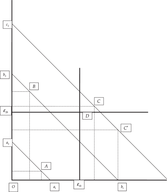
Figure 1: The illustration of calculation of the density of states for 2D electron in the magnetic field in a square.

Let us consider the weak field case, when the Fermi energy $\varepsilon_{\mathrm{F}}>2\varepsilon_{\mathrm{b}}$. If the density of states is determined by averaging over the interval $\Delta$, and the amendments that take the form of the area into account are neglected, the density of states $\widetilde{\mathfrak{N}_{2}(\varepsilon)}$ should be like the one obtained in the work [2]:

$$\widetilde{\mathfrak{N}_{2}(\varepsilon)}=\Theta\left(\frac{m^{2}\omega^{2}S}{4\pi\hbar^{2}}-\varepsilon\right)\left[\frac{\varepsilon}{\Delta^{2}}\right]+\Theta\left(\varepsilon-\frac{m^{2}\omega^{2}S}{4\pi\hbar^{2}}\right)\left[\frac{S}{4\pi}\right].$$ (21)

The integral of the density of states that determines the number of states whose energies are smaller than $\varepsilon$, can be represented as follows:

$$N(\varepsilon>2\varepsilon_{\mathrm{b}})=\int_{0}^{\varepsilon}\widetilde{\mathfrak{N}_{2}(\alpha)}\mathrm{d}\alpha+\int_{0}^{\varepsilon}\left[\mathfrak{N}_{2}(\alpha)-\widetilde{\mathfrak{N}_{2}(\alpha)}\right]\mathrm{d}\alpha,$$ (22)

where $\mathfrak{N}_{2}(\alpha)$ is taken from the formulae (20a, 20b, 20c). The equation for calculation of the Fermi energy $\varepsilon_{\mathrm{F}}$ is obtained by equating $N(\varepsilon_{\mathrm{F}})$ to the total number of electrons $N_{0}$. (For the sake of simplicity, the spin and the Pauli paramagnetism is not considered). This equation can be considered as the implicit definition of the function $\varepsilon_{\mathrm{F}}(H)$. If the second term in the formula (22) is neglected, then:

$$\varepsilon_{\mathrm{F}}(H)=\varepsilon_{\mathrm{F}0}+\varepsilon_{\mathrm{F}1}(H)=\varepsilon_{\mathrm{F}0}+\frac{1}{2\pi}\left(\frac{m\omega L}{\hbar}\right)^{2}=\varepsilon_{\mathrm{F}0}+\frac{1}{2\pi}\left(L\Delta\right)^{2},$$ (23)

where $\varepsilon_{\mathrm{F}0}=4\pi N_{0}/S$ is the Fermi energy in the commonly used theory when there is no magnetic field.

The Fermi energy depends on the magnetic field due to the dependence on the magnetic induction of two parameters: $\varepsilon_{\mathrm{F}}(H)=\varepsilon_{\mathrm{F}}\left[\Delta(H),n_{0}(H)\right]$. These dependencies are qualitatively different: $\Delta(\omega)=m\omega/\hbar$ is the linear function of $H$ that can take on any values, and $n_{0}(\omega)=\left\lceil 4m\omega L^{2}/\pi^{2}\hbar\right\rceil$ can be only integer. Therefore, when the magnetic induction varies in an interval, in which the parameter $n_{0}$ does not vary, the singular points of the function $\mathfrak{N}_{2}(\varepsilon)$ [formulae (20a)–(20c)] move continuously and $\varepsilon_{\mathrm{F}}(H)=\varepsilon_{\mathrm{F}}\left[\Delta(H)\right]$ varies continuously. When the variation of the magnetic induction changes the parameter $n_{0}$, the number of the singular points changes, the spectrum reconstructs, and $\varepsilon_{\mathrm{F}}$ varies non-continuously. Formula (23) that describes the function $\varepsilon_{\mathrm{F}}(H)$ when the density of states is smoothed, should be supplemented by the oscillatory term $\varepsilon_{\mathrm{F}2}(\Delta,n_{0})$. By integration $\mathfrak{N}_{2}(\alpha)$ between the limits $0$ and $\varepsilon_{\mathrm{F}}>2\varepsilon_{\mathrm{b}}$ we obtain:

$$N(\varepsilon_{\mathrm{F}}>2\varepsilon_{\mathrm{b}})={} n_{0}^{2}-\frac{4L\sqrt{\Delta}}{\pi}\left[n_{0}^{3/2}-\sum_{i=0}^{n_{0}}\left(\frac{\varepsilon_{\mathrm{F}}}{\Delta}-i\right)^{1/2}\right]$$

$$+\frac{2L^{2}}{\pi^{2}}\left[\varepsilon_{\mathrm{F}}\arcsin\left(1-\frac{2\Delta n_{0}}{\varepsilon_{\mathrm{F}}}\right)-2\sqrt{\Delta n_{0}(\varepsilon_{\mathrm{F}}-\Delta n_{0})}+2\Delta n_{0}\right].$$ (24)

If $n_{0}(H)-n_{0}(H\pm h)=\pm 1$ then $\Delta(H)-\Delta(H\pm h)=\pm(\pi^{2}/4L^{2})$. Then, the continuous change of $\varepsilon_{\mathrm{F}}$ on this interval is:

$$\delta_{c}\varepsilon_{\mathrm{F}} {}=\frac{\partial\varepsilon_{\mathrm{F}}}{\partial\Delta}\left(\pm\frac{\pi^{2}}{4L^{2}}\right)=-\frac{\partial N}{\partial\Delta}\left(\frac{\partial N}{\partial\varepsilon}\right)^{-1}\left(\pm\frac{\pi^{2}}{4L^{2}}\right)=-\frac{1}{\mathfrak{N}_{2}(\varepsilon_{\mathrm{F}0})}\frac{\partial N}{\partial\Delta}\left(\pm\frac{\pi^{2}}{4L^{2}}\right)$$

$${}\approx-\frac{\pi}{L^{2}}\left(-\frac{n_{0}^{2}}{\Delta}\sqrt{\frac{\varepsilon_{\mathrm{F}0}}{\Delta n_{0}}}\right)\left(\pm\frac{\pi^{2}}{4L^{2}}\right)\approx\pm\frac{2}{L}\sqrt{\varepsilon_{\mathrm{F}0}}=\pm\frac{2}{L^{2}}\sqrt{\pi N_{0}}\,.$$ (25)

This change is much larger than the change that is described by the formula (23). It describes the oscillations of $\varepsilon_{\mathrm{F}2}(\Delta,n_{0})$. At the end of the interval of the continuous change of $\varepsilon_{\mathrm{F}2}(\Delta,n_{0})$, when $n_{0}$ changes by $\pm 1$, the jump of the function $\varepsilon_{\mathrm{F}}$ is:

$$\delta_{j}\varepsilon_{\mathrm{F}}=\pm\frac{\partial\varepsilon_{\mathrm{F}}}{\partial n_{0}}=\mp\frac{\partial N}{\partial n_{0}}\left(\frac{\partial N}{\partial\varepsilon_{\mathrm{F}}}\right)^{-1}=\mp\frac{\pi}{L^{2}}\frac{\partial N}{\partial n_{0}}\approx\mp\frac{\pi}{L^{2}}\left(\frac{n_{0}\varepsilon_{\mathrm{F}0}}{\Delta}\right)=\mp\frac{2}{L}\sqrt{\varepsilon_{\mathrm{F}0}}\,.$$ (26)

When the magnetic field varies, the Fermi energy oscillates with the amplitude  $(\hbar/L)\sqrt{2E_{\mathrm{F}0}/m}$  and  the  period  $\delta H=\pi^{2}\hbar/4L^{2}e_{\mathrm{r}}$.  If $L^{2}\backsim 10^{-4}$ m²  and  $e_{\mathrm{r}}\backsim 10^{-4}e$, this period is of the order of $10^{-6}$ T. The monotonous change of the Fermi energy with the magnetic field is described by the formula (23).

It can be similarly proved that the energy of the electron gas in the magnetic field is described by formula:

$$E=E_{0}+\frac{S^{2}\rho_{0}e_{\mathrm{r}}^{2}H^{2}}{16\pi m}-\frac{S^{3}e_{\mathrm{r}}^{4}H^{4}}{1536\pi^{3}\hbar^{2}m}+E_{\mathrm{osc}}\,.$$ (27)

Here, $E_{0}$ is the energy of the electron gas in the absence of the magnetic field, $\rho_{0}=N_{0}/S$ is the density of gas. This formula differs from the energy of gas that was calculated in the work [2] by an ultimate term $E_{\mathrm{osc}}$ that describes the oscillation of the energy with the amplitude $(4/3\pi)\sqrt{(2mL^{2}/\hbar^{2})E_{\mathrm{F}0}^{3}}\,$.

We take into account that the number of discrete levels $n_{0}$ is an integer and obtain the characteristics of the gas that have the oscillating dependence on the magnetic field. In the commonly used theory, the degenerate multiplicity of equidistant levels $d(H)$ is an integer and is the same for all levels. This quantity differs from $n_{0}$ only by the numerical coefficient that is of the order of unity. When the magnetic field, for example, increases, the gas energy should increase linearly until $d$ is constant. When $d$ increases by 1, the $\lceil N_{0}/d\rceil$ electrons should drop from the top level and the energy decreases by jumps. If the number of electrons on the top level is less than $\lceil N_{0}/d\rceil$, the jump amplitude should be smaller. These decreased jumps should recur, and only this oscillation is considered in the common theory. The 2D electron gas in the magnetic field has been considered in the monographs [3, 4]. The fact that $d(H)$ is an integer is not taken into account in these works. In the work [2] it was shown that the system of equidistant degenerated levels cannot be a correct description of the one-particle spectrum of the electron gas in the magnetic field because in this theory, the angular momentum conservation and the Coulomb interaction are not taken into account.

4 The linear oscillator with zero boundary condition

Let us change the variable in the equation (17) $z=x\sqrt{\Delta}$ and designate $u=-2E/\hbar\omega$. Then, the equation obtains the form of a standard equation for the function of parabolic cylinder (see handbook [5]):

$$\frac{\mathrm{d}^{2}\psi}{\mathrm{d}z^{2}}-\left(\frac{z^{2}}{4}+u\right)\psi=0.$$ (28)

The even and odd solutions of this equation are:

$$\psi_{\mathrm{e}}=A_{\mathrm{e}}\exp\left(-\frac{z^{2}}{4}\right)\Phi\left(\frac{u}{2}+\frac{1}{4},\frac{1}{2};\frac{z^{2}}{2}\right);$$

$$\psi_{\mathrm{o}}=A_{\mathrm{o}}z\exp\left(-\frac{z^{2}}{4}\right)\Phi\left(\frac{u}{2}+\frac{3}{4},\frac{3}{2};\frac{z^{2}}{2}\right).$$ (29)

Here, $\Phi(a,c;t)$ is the degenerate hypergeometric function (DHF), $A_{\mathrm{e(o)}}$ are the normalization constants. The middle of the line segment is zero of the coordinate. The length of the segment is $2L$. To satisfy the boundary condition (18), the eigenvalue $u$ should be such that

$$\Phi\left(\frac{u}{2}+\frac{1}{4},\frac{1}{2};z_{L}^{2}\right)=0,\quad\mbox{or}\quad\Phi\left(\frac{u}{2}+\frac{3}{4},\frac{3}{2};z_{L}^{2}\right)=0;\qquad z_{L}^{2}=\frac{m\omega L^{2}}{2\hbar}\,.$$ (30)

This problem could not be consequently considered because in the description of nulls of DHF in all mathematical handbooks (see for example [5],[6]) an inaccuracy takes place. It is proved that, if $a<0$ and $c>0$, the number of nulls of the function $\Phi(a,c;t)$ is equal to $(-a)$, if it is integer, and is equal to $\lceil-a\rceil+1$, if $(-a)$ is non-integer. It is also proved that nulls are described approximately by the formula:

$$\xi_{i}(a,c)=\frac{1}{2c-4a}j_{c-1,i}^{2}\,,$$ (31)

if $|a|\gg 1$. Here, $\xi_{i}(a,c)$ is the null of DHF that has the number $i\leqslant\lceil-a\rceil+1$ in the order of increasing, $j_{c-1,i}^{2}$ is the square of the respective null of the Bessel function of the first kind $J_{c-1}(x)$. If this were so, the greatest nulls of the functions that are the solutions of the considered problem should be linear functions of the eigenvalue $u$. Then, the smallest eigenvalues should be $\sim m\omega L^{2}/2\hbar$, i.e., the spectrum should begin from very large values of energy. In the work [7] (see also [2]) it was shown that the formula (31) describes each null of the DHF only when $(-a)$ is integer. Then, the Kummer power series that describes DHF terminates at the term with number $1-a$, and the DHF in the formulae (30) are proportional to the Laguerre polynomials $L_{(-a)}^{\pm 1/2}(z_{L}^{2})$. The number of nulls of these polynomials is $k=-a$. All these nulls are real, positive, simple and are described by the formula (31). Let us consider the DHF $\Phi(a,1/2;t)$ when $a=-k-\gamma$, where $k$ is an integer and $0<\gamma<1$. Then, this DHF has $k+1$ nulls of which $k$ nulls come out of the nulls of Laguerre polynomial that are diminished by quantities which are proportional to $\gamma$. These nulls are described by the formula (31). The null that has the number $k+1$ is the largest, and its dependence on $\gamma$ should possess the following properties:

$$\lim_{\gamma\to 0}\left[\xi_{k+1}(-k-\gamma,1/2)\right]\to\infty,\qquad\lim_{\gamma\to 1}\left[\xi_{k+1}(-k-\gamma,1/2)\right]=\xi_{k+1}(-k-1,1/2).$$ (32)

To calculate $\xi_{k+1}(-k-\gamma,1/2)$ when $\gamma$ is small, the DHF $\Phi(-k-\gamma,1/2;t)$ should be changed by the asymptotic expression. The Kummer power series would be represented as follows:

$$\Phi(-k-\gamma,1/2;t)=P_{k}^{1/2}(\gamma,t)-\gamma Q_{k}^{1/2}(\gamma,t)-\gamma(1-\gamma)T_{k}^{1/2}(\gamma,t).$$ (33)

Here, $P_{k}^{1/2}(\gamma,t)$ is a polynomial that can be obtained from the Laguerre polynomial $L_{k}^{-1/2}(t)$ by changing $k\to k+\gamma$ in its coefficients, $\gamma Q_{k}^{1/2}(\gamma,t)$ is the next term of the Kummer series that is proportional to $\gamma$, $\gamma(1-\gamma)T^{1/2}_{k}(\gamma,t)$ is the remaining infinite series that also is proportional to $\gamma$. It can be shown that when $t$ is large and $\gamma$ is small

$$\gamma(1-\gamma)T_{k}^{1/2}(\gamma,t)\approx\gamma(-1)^{k}(1+\gamma)_{k}\sqrt{\pi}(t)^{-n-1/2}\exp(t).$$ (34)

Here, $(b)_{i}=b(b+1)\cdots(b+i-1)$ is the Pochhammer symbol. The second term in the formula (33) can be neglected. The polynomial $P_{k}^{1/2}(\gamma,t)$ can be changed by the last term, when $t$ is large:

$$P_{k}^{1/2}(\gamma,t)\approx\frac{(-k-\gamma)_{k}t^{k}}{(1/2)_{k}k!}=(-1)^{k}\frac{(1+\gamma)_{k}t^{k}}{(1/2)_{k}k!}\,.$$ (35)

We set the obtained approximate expression for DHF equal to zero. This equation defines the quantity $\gamma$ as the function of $\xi_{k+1}(-k-\gamma,1/2)=t_{0}$:

$$\gamma_{1/2}(k,t_{0})=\left[k!\Gamma\left(k+\frac{1}{2}\right)\right]^{-1}t_{0}^{2k+1/2}\exp(-t_{0}).$$ (36)

For the boundary condition to be satisfied by the largest null of DHF $\Phi(-k-\gamma,1/2;t)$, this null should be larger than $\xi_{k+1}(-k-1,1/2)$, i.e.,

$$t_{0}=\frac{m\omega L^{2}}{2\hbar}>\frac{1}{1+4(k+1)}j_{-1/2,k+1}^{2}\,,$$ (37)

$j_{-1/2,l}=\pi(l-1/2)$, where $l$ is integer. Therefore, the boundary condition can be satisfied by the largest null of DHF, if the value of $k$ is not greater than $k_{0}$:

$$k_{0}\approx\left\lceil\frac{2m\omega L^{2}}{\pi^{2}\hbar}\right\rceil.$$ (38)

This is the approximate formula, but the operation of taking an integer part emphasizes that $k_{0}$ is an integer, and when the frequency changes, this quantity does not change continuously and takes only integer values. The eigenvalues for the even solutions:

$$E_{\mathrm{e}}=\hbar\omega\left(k_{\mathrm{e}}+\frac{1}{4}+\gamma_{1/2}(k_{\mathrm{e}})\right).$$ (39)

If $k>k_{0}$, the boundary condition can be satisfied by one of the nulls of DHF that is described by the formula (31) when $(-a)>k_{0}$. To calculate these values $a$, i.e., the eigenvalues of energy, we use the first term of the expansion DHF over the Bessel functions (see monograph [6]). This expansion is rapidly convergent, when $|a|$ is large. We obtain the following even solution of the equation (28):

$$\psi_{\mathrm{e}}\approx A_{\mathrm{e}}\Gamma\left(\frac{1}{2}\right)\left(-\frac{uz^{2}}{4}\right)^{1/4}\!\!J_{-1/2}\left(2\sqrt{-uz^{2}/4}\right)=A_{\mathrm{e}}\cos\left(z\sqrt{2E_{\mathrm{e}}/\hbar\omega}\right)=A_{\mathrm{e}}\cos\left(\frac{x}{\hbar}\sqrt{2mE_{\mathrm{e}}}\right).$$ (40)

The eigenvalues of the energy for which these wave functions are equal to zero at the ends of a segment are obtained:

$$E_{\mathrm{e}}=\frac{\pi^{2}\hbar^{2}}{2mL^{2}}\left(k_{\mathrm{e}}+\frac{1}{2}\right)^{2}=\frac{\pi^{2}\hbar^{2}}{8mL^{2}}(2k_{\mathrm{e}}+1)^{2},\qquad k_{\mathrm{e}}>k_{0}\,.$$ (41)

A similar computation for the odd wave function leads to the results:

$$\gamma_{3/2}(k,t_{0})=\left[k!\Gamma\left(k+\frac{3}{2}\right)\right]^{-1}t_{0}^{2k+3/2}\exp(-t_{0}),\qquad E_{\mathrm{o}}=\hbar\omega\left(k_{\mathrm{o}}+\frac{3}{4}+\gamma_{3/2}(k_{\mathrm{o}})\right);$$ (42)

$$\psi_{\mathrm{o}}\approx A_{\mathrm{o}}\sin\left(\frac{x}{\hbar}\sqrt{2mE_{\mathrm{o}}}\right),\qquad E_{\mathrm{o}}=\frac{\pi^{2}\hbar^{2}}{2mL^{2}}k_{\mathrm{o}}^{2}=\frac{\pi^{2}\hbar^{2}}{8mL^{2}}(2k_{\mathrm{o}})^{2},\quad k_{\mathrm{o}}>k_{0}\,.$$

The formulae for the spectrum can be unified, if it is taken into account that the amendments $\gamma$ can be neglected everywhere except the immediate neighborhood of $k_{0}$:

$$E_{n}=\frac{\hbar\omega}{2}\left(n+\frac{1}{2}\right),\qquad n<n_{0}=2k_{0};\qquad E_{n}=\frac{\pi^{2}\hbar^{2}}{8mL^{2}}n^{2},\qquad n>n_{0}\,.$$ (43)

If in the equation (17) we change $\omega=2\omega_{0}$, this equation will gain the form of a standard equation for the linear oscillator with frequency $\omega_{0}$. If $L\to\infty$, the boundary condition (18) should be changed by the requirement of normability of the wave functions. Then, the obtained solution of the problem turns into the common solution for the linear oscillator. When $n>n_{0}$, the approximate solutions (40) and (42) are the common solutions for the particle in the rectangular potential well. However, the energy $E_{\mathrm{b}}=\hbar\omega n_{0}/2=2m\omega^{2}L^{2}/\pi^{2}$ that is the boundary between the two kinds of solutions does not coincide with the value of the potential energy at the boundary of the area as might be expected from the quasiclassical consideration.

Ukrainian 0

Густина одночастинкових станiв для 2D електронного газу у магнiтному полi I.М. Дубровський

             
Iнститут металофiзики, бульв. Вернадського 36, Київ 03680, Україна

References

- [1] Courant R., Hilbert D., Methods of Mathematical Physics, Vol. 1, Interscience, New York, 1953.
- [2] Dubrovskyi I., In: Thermodynamics. Interaction Studies — Solids, Liquids and Gases, Moreno-Pirajan J.C. (Ed.), InTech, 2011, Chap. 17; doi:10.5772/823.
- [3] Abrikosov A.A., Introduction to the Theory of Metals, Amsterdam, North-Holland, 1986.
- [4] Shoenberg D., Magnetic Oscillations in Metals, Cambridge University Press, Cambridge, 1984.
- [5] Handbook of Mathematical Functions with Formulas, Graphs, and Mathematical Tables. National Bureau of Standards Applied Mathematics Series Vol. 55, Abramovitz M., Stegun I.A. (Eds.), U.S. Government Printing Office, Washington, D.C., 1964.
- [6] Bateman H., Erdèlyi A., Higher Transcendental Functions, Vol. 1, Robert E. Krieger, 1981.
- [7] Dubrovskii I.M., Condens. Matter Phys., 2006, 9, 645.
Ukrainian \adddialect\l@ukrainian0 \l@ukrainian