Herschel far-infrared observations of the Carina Nebula Complex

Abstract

Context. The star formation process in large clusters/associations can be strongly influenced by the feedback from high mass stars. Whether the resulting net effect of the feedback is predominantly negative (cloud dispersal) or positive (triggering of star formation due to cloud compression) is still an open question.

Aims. The Carina Nebula complex (CNC) represents one of the most massive star-forming regions in our Galaxy. We use our Herschel far-infrared observations to study the properties of the clouds over the entire area of the CNC (with a diameter of $\approx 3.2\degr$, which corresponds to $\approx 125$ pc at the distance of 2.3 kpc). The good angular resolution ($10^{\prime\prime}-36^{\prime\prime}$) of the Herschel maps corresponds to physical scales of 0.1 – 0.4 pc, and allows us to analyze the small-scale (i.e. clump-size) structures of the clouds.

Methods. The full extent of the CNC was mapped with PACS and SPIRE in the 70, 160, 250, 350, and $500\,\mu$m bands. We determine temperatures and column densities at each point in this maps by modeling the observed far-infrared spectral energy distributions. We also derive a map showing the strength of the UV radiation field. We investigate the relation between the cloud properties and the spatial distribution of the high-mass stars, and compute total cloud masses for different density thresholds.

Results. Our Herschel maps resolve, for the first time, the small-scale structure of the dense clouds over the entire spatial extent of the CNC. Several particularly interesting regions, including the prominent pillars south of $\eta$ Car, are analyzed in detail. We compare the cloud masses derived from the Herschel data to previous mass estimates based on sub-mm and molecular line data. Our maps also reveal a peculiar “wave”-like pattern in the northern part of the Carina Nebula. Finally, we characterize two prominent cloud complexes at the periphery of our Herschel maps, which are probably molecular clouds in the Galactic background.

Conclusions. We find that the density and temperature structure of the clouds in most parts of the CNC is dominated by the strong feedback from the numerous massive stars, rather than random turbulence. Comparing the cloud mass and the star formation rate derived for the CNC to other Galactic star forming regions suggests that the CNC is forming stars in an particularly efficient way. We suggest this to be a consequence of triggered star formation by radiative cloud compression.

1 Introduction

The Carina Nebula complex (CNC hereafter) (e.g. Smith & Brooks 2008, for an overview of the region) is one of the richest and largest high-mass star forming regions in our Galaxy. At a moderate distance of 2.3 kpc, it contains at least 65 O-type stars (Smith 2006) and four Wolf-Rayet stars (see e.g. Smith & Conti 2008).
The CNC extends over at least $\sim 80$ pc, which corresponds to more than 2 degrees on the sky, demonstrating that wide-field surveys are necessary in order to obtain a comprehensive information on the full star forming complex. Several wide-field surveys of the CNC have recently been carried out at different wavelengths. The combination of a large Chandra X-ray survey (see Townsley et al. 2011b) with a deep near-infrared survey Preibisch et al. (2011c, b) and Spitzer mid-infrared observations (Smith et al. 2010; Povich et al. 2011) provided comprehensive information about the young stellar populations. Our sub-millimeter survey of the CNC with LABOCA at the APEX telescope revealed the structure of the cold and dense clouds in the complex in detail (Preibisch et al. 2011a).

The CNC is an interesting region in which to study the feedback effects of the numerous very massive and luminous stars on the surrounding clouds. The strong ionizing radiation and the powerful winds of the high-mass stars affect the clouds in very different ways: on the one hand, the process of photoevaporation at strongly irradiated cloud surfaces can disperse even rather massive clouds on relatively short timescales; transforming dense molecular clouds into warm/hot low-density atomic gas will strongly limit the potential for further star formation. On the other hand, the compression of clouds by irradiation and by expanding bubbles driven by evolving HII regions (e.g. Deharveng et al. 2005) or stellar winds can produce gravitationally unstable density peaks and lead to triggered star formation (e.g. Smith et al. 2010). The detailed balance of these two opposing processes determines the evolution of the complex and decides, how much of the original cloud mass is actually transformed into stars and what fraction is dispersed by the feedback. In order to study this interaction between the stars and the surrounding clouds, a comprehensive characterization of the cloud structure and temperature is a fundamental requirement.

The ESA Herschel Space Observatory (Pilbratt et al. 2010) is ideally suited to map the far-infrared emission of the warm and cool/cold molecular clouds and is currently observing many galactic (and extragalactic) star forming regions. We have used the Herschel Observatory to perform a wide-field ($\ga 5$ square-degrees) survey of the CNC (P.I.: Th. Preibisch) that covers the entire spatial extent of the clouds. Far-infrared photometric maps were obtained with PACS (Poglitsch et al. 2010) at 70 and 160 $\mu$m, and with SPIRE (Griffin et al. 2010) at 250, 350, and $500\leavevmode\nobreak\ \mu$m. A first analysis of these Herschel observations, focusing on the large scale structures and global properties, has been presented in Preibisch et al. (2012) (Paper I in the following text). A detailed study of the young stellar and protostellar population detected as point-sources in the Herschel maps is described in Gaczkowski et al. (2013). The properties of the clouds around the prominent HII region Gum 31, located just north-west of the central Carina Nebula, as derived from these Herschel and other observations are studied in Ohlendorf et al. (2013). In this paper, we present a detailed analysis of the temperature and column density of the small-scale structures of the entire CNC.

This paper is organized as follows: in Section 2 we briefly summarize the Herschel PACS and SPIRE observations, data reduction and the final temperature and column density maps of the CNC. In Section 3 we compute the temperature, column density and UV-flux maps of the clouds. In Section 4 we present a detailed analysis of the cloud structures resolved by Herschel in the CNC., e.g. the southern pillars. We discuss, in Section 6, the comparison between dense and diffuse gas, the relation between dust and gas mass estimates, the strength of the radiative feedback and the CNC as a link between local and extragalactic star formation. A summary of our results and conclusions is given in Section 7.

2 The Herschel PACS and SPIRE maps of the Carina Nebula Complex

2.1 Observations and Data Reduction

The CNC has been observed on December 26, 2010 using the parallel fast scan mode at $60^{\prime\prime}$/s, obtaining simultaneously $70\,\mu$m and $160\,\mu$m images with PACS, and 250, 350, and 500 $\mu$m maps with SPIRE.

The scan maps cover an area of 2.8${}^{\circ}\times 2.8^{\circ}$, which corresponds to about 110 pc $\times$ 110 pc at the distance of the CNC. The data reduction has been carried out combining the HIPE (v. 7.0; Ott 2010) with the SCANAMORPHOS package (v. 13.0; Roussel 2012). All the details of the reduction can be found in Paper I. We here only emphasize that we used the option galactic in SCANAMORPHOS which preserves the brightness gradient over the field. The final angular resolution of the PACS/Herschel  maps was $\approx 12^{\prime\prime}-16^{\prime\prime}$, while for the SPIRE/Herschel  maps $\approx 20^{\prime\prime}-36^{\prime\prime}$.

2.2 Calibration

The observations and mosaics of the CNC have been previously presented in Paper I. In this work an additional effort to calibrate the final mosaic has been done by discussing the effect of the large scale flux loss and taking into account the color correction, which might influence our further analysis. In the first case, it is important to recall that Herschel is a warm instrument, not designed to obtain absolute fluxes. The warm emission from the telescope’s mirror is removed using a high-pass filtering during the data reduction. However, this step might remove some large scale emission in the final mosaics. The flux loss can only be estimated by extrapolating the Herschel fluxes to the wavelengths observed by a cold telescope, such as e.g. Planck.

Another possibility is to obtain the contributions from background and foreground material estimating the dust in foreground/background gas that is traced by H I, for the atomic emission, and CO, for the molecular emission. This approach has been presented by Rivera-Ingraham et al. (2013).

Since the Planck data are not yet publicly available and we do not have H I and CO spectral data of the CNC, we compared our Herschel 70 $\mu$m map to the IRAS 60 $\mu$m map. This approach was already used in Paper I and the details can be found there.

We also use another approach, which consists in removing the local background at each wavelength, by assuming an average value over the field (see e.g. Stutz et al. 2010). In this way we only take into account the Herschel emission above this local background. This was computed in a region of the PACS and SPIRE maps outside the CNC where there was no cloud emission. We find that the local background is 0.0005 Jy/arcsec².

We checked whether the subtraction of the local background estimated was affecting our result on the temperature structure.

Both approaches show that the large scale flux loss can introduce an error negligible compared to a conservative calibration error of 20% of the flux adopted in our work.

The second calibration step taken into account is the color correction. This correction can affect the Herschel photometry at the shortest wavelengths in the case of low temperaturesTo correct the PACS fluxes we used the first temperature map obtained by fitting the SED on the uncorrected Herschel fluxes ($F_{unc}$). For a given temperature, we applied the color corrections $cc_{pacs70}$ and $cc_{pacs160}$ listed in the PACS manual¹; the corrected flux $F_{corr}$ is computed as $F_{corr}=F_{unc}/cc_{pacs}$.

In a second step the fit of the SED has been repeated using the color-corrected fluxes.

Between the two iterations the temperature map differs of about 0.1 K in the coldest part of the CNC (T$\sim$16 K). For warmer parts the correction was less than 0.1 K.

We checked the effect of the color-correction on the SPIRE photometry. The SPIRE color corrections are obtained checking the slope $\alpha$ of the spectral energy distribution (SED hereafter) between 250 and 500 $\mu$m. From an average spectral index value of about 2.4 over the entire Herschel mosaic, the color correction would have ranged between 1.02 and 0.97 . This correction is hence negligible.

3 Analysis

3.1 Temperature and column density of the clouds

In this section we describe in detail the procedure to obtain a precise temperature and column density map of the CNC. The most reliable and powerful approach to derive the dust temperature and density maps is fitting, pixel by pixel, the SED to the fluxes in the 5 Herschel bands. The final Herschel mosaics at 70, 160, 250, 350, and 500 $\mu$m (derived as previously described) have been convolved to the angular resolution of the 500 $\mu$m image, using the procedure presented in Stutz et al. (2010) and the kernels from Aniano et al. (2011).

Since the nebula is optically thin at all the Herschel wavelengths (Preibisch et al. 2011b), the emission of the nebula is $B_{\nu}(T)\cdot\tau$, where $B_{\nu}$ is the Planck function at a temperature $T$ and $\tau$ is the optical depth, which is proportional to the dust mass absorption coefficient, $k_{\nu}$. From the models presented in Ossenkopf & Henning (1994), we choose a dust model with a highest $\beta$ value (i.e. 1.9) which is representative to describe a dense molecular cloud. This model has a standard MRN-distribution for diffuse interstellar medium (Draine & Lee 1984) composed of grains without ice mantels. We used the tabulated values of $k_{\nu}$ [cm²/g] for such a model and interpolated at the Herschel wavelengths. In Table 1 we show the values of $k_{\nu}$ that we obtained.

Table 1: Values of the dust mass absorption coefficient, $k_{\nu}$ interpolated at the Heschel bands from the model of Ossenkopf & Henning (1994) with a $\beta$ value of 1.9.

$\lambda$	$70\,\mu$m	$160\,\mu$m	$250\,\mu$m	$350\,\mu$m	$500\,\mu$m
$k_{\nu}$ [cm2/g]	118.0	24.8	11.6	5.9	2.9

The fit of the SED is obtained by using a black-body leaving as free parameters the temperature $T$ and the surface density $\Sigma\,[{\rm g/cm^{2}}]$. A similar approach to obtain temperature and column density has been applied for the analysis of the HOBYS key project by e.g. Hennemann et al. (2012) and the Gould Belt key program by e.g. Palmeirim et al. (2013).

The final temperature and density maps are obtained from the Herschel/PACS and SPIRE color corrected mosaics.

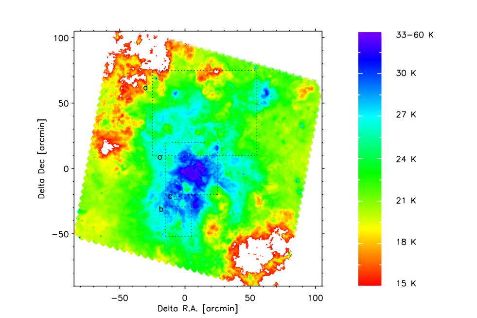
Figure 1: Temperature map of the Carina nebula. The dashed boxes represent: the central region around $\eta$ Car (box ‘a’), the Southern Pillars region (box ‘b’), the Treasure Chest Cluster (box ‘c’), and the ‘wave’ pattern (box ‘d’). These regions are analyzed in detail in Figures 4, 5, 7, and 8. The center of the figure corresponds to the position $(\alpha_{\rm J2000},\,\delta_{\rm J2000})\,=\,(10^{\rm h}\,45^{\rm m}\,21^{\rm s},\,-59\degr\,34^{\prime}\,20^{\prime\prime})$.

The final temperature map of the CNC is shown in Figure 1. We find that the average temperature of most of the nebula is about 30 K, ranging between 35-40 K in the central clouds and 26 K in the clouds at the edge of the nebula.

In Paper I we presented a first color-temperature map of the CNC, derived from the ratio of the $70\,\mu$m and $160\,\mu$m images. The warmer cloud surface temperature is traced with the best resolution, since the convolution of the two original mosaics has been done on the PACS 160 $\mu$m.

However, a color temperature may be less well suited for dense clouds where much of the 70 $\mu$m - 160 $\mu$m emission comes from the warmer cloud surfaces. In this case, the temperature computed by the SED fitting computes the beam averaged temperature among the line of sight and it is more sensitive to the densest (and thus coolest) central parts of clouds.

We find that the temperature computed in Paper I show values up to $\sim 5\%$ higher than the values with the SED fitting. This result was already expected because the color temperature is biased to the warmer cloud surface.

The second free parameter of the SED fitting is the dust surface density, $\Sigma$. The column density N_H is obtained as following

$$N_{\rm H}=2N_{\rm H_{2}}=\frac{2\cdot\Sigma\cdot R}{m_{\rm H}\cdot\mu_{\rm H_{2}}}$$ (1)

where m_H is the hydrogen mass and $\mu_{\rm H_{2}}$ is the mean molecular weight (i.e. 2.8). Multiplying by the gas-to-dust mass ratio $R$ (assumed to be 100), we obtain the total column density.

In Figure 2 we show the resulting total column density map. The median value over the entire CNC (2.3${}^{\circ}\times$2.3^∘) is $1.8\times 10^{21}\,{\rm cm}^{-2}$, while the mean value is $2.3\times 10^{21}\,{\rm cm}^{-2}$.

We find column densities up to $5\times 10^{22}\,{\rm cm^{-2}}$. From the Southern Pillars, in the South-East direction from Carina, there is an almost continuos structure with density of about $3.0-5.5\times 10^{21}\,{\rm cm^{-2}}$. In the opposite direction, north-east to south-west from the Carina Nebula, the density is lower, down to $9\times 10^{20}\,{\rm cm^{-2}}$.

In particular the large elongated bubble south-west of $\eta$ Car is a quite prominent empty region already described in Paper I.

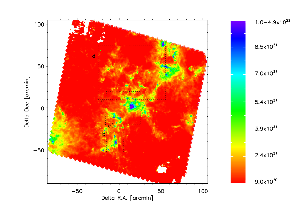
Figure 2: Column density map of the Carina nebula. The color scale is expressed in ${\rm cm^{-2}}$. The dashed boxes represent: the central region around $\eta$ Car (box ‘a’), the Southern Pillars region (box ‘b’), the Treasure Chest Cluster (box ‘c’), and the ‘wave’ pattern (box ‘d’). These regions are analyzed in detail in Figures 4, 5, 7, and 8. The center of the figure corresponds to the position $(\alpha_{\rm J2000},\,\delta_{\rm J2000})\,=\,(10^{\rm h}\,45^{\rm m}\,21^{\rm s},\,-59\degr\,34^{\prime}\,20^{\prime\prime})$.

We note that a conservative calibration error of 20% in the intensity causes just 5-10% uncertainty in the derived temperatures, and at T$\sim$20 K, a 5% error in temperature will cause a $\leq$10% error in the derived column density.

3.2 Determination of the UV-flux

The surfaces of the clouds we see in the FIR maps are mainly heated by the far-UV (FUV) radiation from the hot stars in the complex; the FUV photons are very efficiently absorbed by the dust grains and thus heat the dust to temperatures well above the “general ISM” cloud temperatures of $\sim 18$ K (see, e.g. Hollenbach & Tielens 1999). Since the heated dust grains cool by emitting the FIR radiation we can observe with Herschel, one can estimate the strength of the FUV radiation field from the observed intensity of the FIR radiation. This yields important quantitative information about the local strength of the radiative feedback from the massive stars.

For a few selected clouds in the CNC, the strength of the FUV irradiation has been already determined in previous studies. Brooks et al. (2003) investigated the photo-dissociation region (PDR) at the eastern front of the dense cloud west of Tr 14 and found that the FUV field is 600 to 10 000 times stronger than the so-called Habing field, i.e. the average intensity of the local Galactic FUV ($912\,\AA-2400\,\AA$) flux of $1.6\times 10^{-3}\,{\rm erg\,cm^{-2}\,s^{-1}}$ (Habing 1968). Kramer et al. (2008) derived an independent estimate of the FUV irradiation at the same cloud front, finding values of 3400 to 8500 times the Habing field. For for another cloud south of $\eta$ Car, these authors found irradiation values of 680 to 1360 times the Habing field.

Using the approach described in more detail by Kramer et al. (2008), we computed the FUV radiation field for all clouds in the CNC from the observed intensity of the FIR radiation in our Herschel maps. For this, we used our PACS 70 $\mu$m and 160 $\mu$m band maps to determine the total intensity integrated over the 60 $\mu$m to 200 $\mu$m FIR range. Since these two bands cover the peak of the FIR emission spectrum of the irradiated clouds, they constitute a good tracer of the radiation from the heated cloud surfaces, and also provide very good angular resolution. We did not include the longer wavelength SPIRE bands, firstly because the angular resolution in these bands is considerably worse, and secondly because the emission at $\ga 250\,\mu$m is probably dominated by the thermal emission from cold dense clumps, that are well shielded from the ambient FUV field; the emission from these very dense and cold cloud structures does thus not directly trace the FUV irradiation. In any case, the contribution of the SPIRE bands to the integrated intensity would be quite small.

To determine the total $60-200$ $\mu$m FIR intensity, $I_{\rm FIR}$, we first smoothed the PACS 70 $\mu$m map to the angular resolution of the PACS 160 $\mu$m map and created maps with a pixel size of $4.5^{\prime\prime}$ (corresponding to 0.049 pc). For each pixel in this map, we then multiplied the specific intensity in the two bands by the bandwidth ($60-80\,\mu$m and $125-200\,\mu$m; see PACS MANUAL). In order to fill the gap from $80\,\mu$m to $125\,\mu$m, we took the average of the 70 $\mu$m and 160 $\mu$m intensities and multiplied it by the corresponding band width. The resulting sum is a measure of the total $60-200$ $\mu$m FIR intensity ($I_{\rm FIR}$).

Following the arguments of Kramer et al. (2008), the FUV field strength can then be computed via the relation

$$G_{0}=\frac{4\pi\,I_{\rm FIR}}{1.6\times 10^{-3}\,{\rm erg\,cm^{-2}\,s^{-1}}}$$ (2)

where the denominator contains the Habing field.

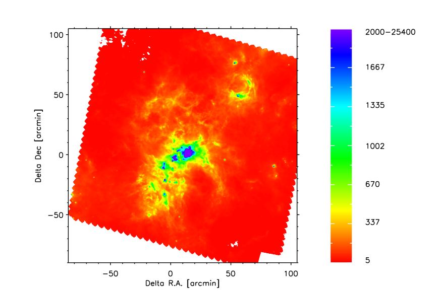
Figure 3: Far-ultraviolet (FUV) flux $G_{0}$ (in units of the Habing field) of the Carina Nebula Complex . The center of the figure corresponds to the position $(\alpha_{\rm J2000},\,\delta_{\rm J2000})\,=\,(10^{\rm h}\,45^{\rm m}\,21^{\rm s},\,-59\degr\,34^{\prime}\,20^{\prime\prime})$.

The resulting map of the derived FUV field in units of the Habing field is shown in Figure 3. In the enlargements of the FUV map, shown in Figures 4, 5, and 7, we also overplotted the positions of the known high-mass stars in the CNC. For the individual clouds already studied by Kramer et al. (2008) and Brooks et al. (2003), our values agree well with the previous, independent determinations by these authors.

Our map shows that nearly all cloud surfaces in the CNC are irradiated with $G_{0}$ values above $\sim 300$, which seems reasonable for a region containing such a large number of OB stars (Hollenbach et al. 1991). Particularly high G₀ values, between $\approx 3000$ and $\approx 10\,000$, are found for the massive cloud to the west of Tr 14, Values above 3000 are found in the Keyhole Nebula, several clouds to the north and west of Tr 14, and a pillar south-east of $\eta$ Car.

It is interesting to compare our map to the results of Smith (2006), who computed an estimate of the radial dependence of the average FUV radiation field from the spectral type of each high mass star in the central clusters (i.e. Tr 14, Tr 15 and Tr 16). At distances larger than 10 pc from the center of the Nebula, the ionizing source can be treated as a point-like source, and the ionizing flux drops as $r^{-2}$. The local radiation within few parsec from each high mass cluster is found to be more important than the cumulative effect from all the clusters. The FUV radiation computed by Smith (2006) is consistent with the values we found: between 100 and 1000 at distances larger than 10 pc from the center, and values up to 10⁴-10⁵ near the individual clusters.

In the Southern Pillars area, which is further away from the hot stars in the central clusters, we find G₀ values around 1000 and up to 2000 along the pillar surfaces.

In most parts of our map area, the spatial distribution of the derived FUV intensities correlates well with the cloud temperatures. However, in some locations, clear differences can be seen. One prominent case is the Gum 31 region, in the north-western part of our maps (see Ohlendorf et al. 2013, for a comprehensive study of this region). While the peak of the cloud temperature is found in the diffuse gas around the OB stars in the central cluster NGC 3324, the highest FUV intensities are found at the western and southern rim of the bubble surrounding NGC 3324.

4 Detailed structure of the clouds in the Carina Nebula Complex

In this section we characterize particularly interesting small-scale structures in the CNC which are resolved in the Herschel maps. In particular we will analyze the central part of the CNC, the Southern Pillars region and the Treasure Chest Cluster .

4.1 Central part

An enlargement of a $23$ pc $\times\,26$ pc region around $\eta$ Car is shown in Figure 4. Our Herschel maps provide sufficient angular resolution to investigate the temperature and column density structure of the clouds around $\eta$ Car in detail.

In the southern direction from $\eta$ Car a dense molecular cloud ridge is resolved in the IRAC image and column density map. The temperature is not homogeneous around $\eta$ Car: in the North-West direction from $\eta$ Car the temperature is higher, ranging between 35 and 45 K; in the South-East direction the temperature is lower, between 25 and 35 K.

In this region, there are the young clusters, Trumpler 14, 15 and 16, which host about 80% of the high mass stars of the entire complex. This is also the hottest region of the nebula with temperatures ranging between 30 and 50 K (excluding the position of $\eta$ Car itself which reaches values of 60 K).

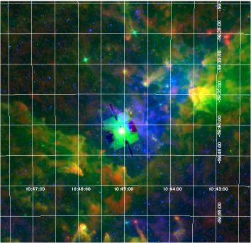
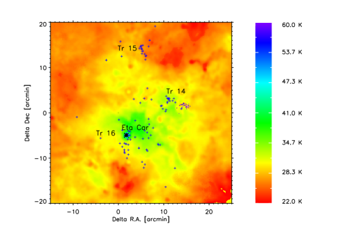
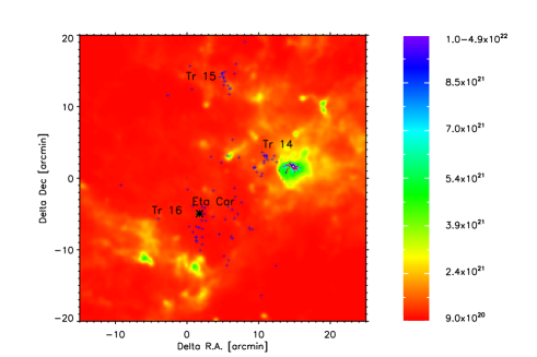
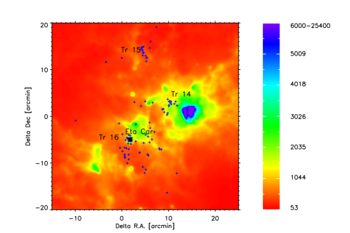
Figure 4: Upper left: Composite optical DSS (in blue), Spitzer IRAC4 (in green), and LABOCA (in red) image of the central part of the Carina Nebula Complex around $\eta$ Car (box ‘a’ in Fig. 1 and 2). Upper right: Temperature map of the central part of the Carina Nebula Complex. Lower: Column density map, expressed in ${\rm cm^{-2}}$ (left) and Far-ultraviolet (FUV) flux $G_{0}$ (in units of the Habing field) (right) of the enlargement around $\eta$ Car. The blue crosses represent the positions of the high mass stars in this region and the black star the position of $\eta$ Car.

In particular, the clouds in and around the stellar cluster Tr 16, which hosts most of the high mass stars in the nebula including $\eta$ Car, have temperatures between 29 and 48 K. Tr 14, which hosts 20 O-type stars, shows cloud temperatures of 30–33 K, and Tr 15, with 6 O-type stars, displays a lower temperature of 26–28 K. The local temperature of the cloud is hence related to the number of high mass stars.

The column density map of the molecular cloud around the clusters shows low values of about $9.0\times 10^{20}\,{\rm cm^{\rm-2}}$. The molecular cloud structures at the edges of the clusters are colder ($\sim 23$ K) and denser $\sim 3.9\times 10^{21}\,{\rm cm^{\rm-2}}$ compared to the central part. The most prominent cloud West of Tr 14 has a temperature of about 30 K and a decrease in density from the inner to the edge part.

4.2 The Southern Pillars

In the Southern Pillars region of the CNC, the temperature ranges between 21 K and 30 K. For a few of the most prominent pillars, we analyze the temperature and density profiles in detail. In Figure 5 an image of the Southern Pillars is compared with the temperature and column density maps. All the structures in the composite image in Figure 5 are reproduced in the density map. The two most prominent pillars (Pillar A and Pillar B in Fig. 5) have a projected angular separation of about 4^′′. In the East direction from Pillar A and Pillar B another pillar is evident in the composite image of Figure 5. This is only barely visible in the density map, while in the temperature map only a slightly colder temperature compared to the local environment is seen at the head of the pillar. The projected size of both, Pillar A and Pillar B, is about 5 pc. The head of the pillars points in the direction of the central stellar cluster Tr 16. Their column densities range from $\sim 3.0\times 10^{21}\,{\rm cm^{\rm-2}}$ at the edge of the pillar structure, up to $\sim 10\times 10^{21}\,{\rm cm^{\rm-2}}$ at the peak of density in the central part of Pillar B. In order to analyze the temperature and density profiles along the pillars, we show the run of temperature and column density along cuts perpendicularly to their main axis, spaced by $\sim$1$\arcmin$ from the bottom to their head. While the temperature profile always decreases from the edge to the center of the pillar, the density profile increases and the maximum of the density in the pillar’s center corresponds to the minimum temperature. The temperature varies by 2 K according to their position on the pillars: cooler at the bottom of the pillar and hotter at their head. The Pillar A is found to be about 2 K cooler than Pillar B. A possible explanation is that Pillar B is closer to the stellar cluster Bochum 11 which harbours 5 high-mass stars. The temperature and density profile of Pillar A suggests that it consists of two partly resolved pillars: the first and third sections show a double peak in both temperature and density profiles, while the second and fourth sections show only one peak which traces one of the two here unresolved pillars.

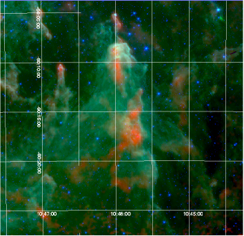
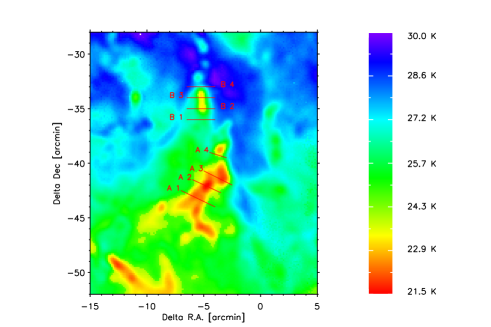
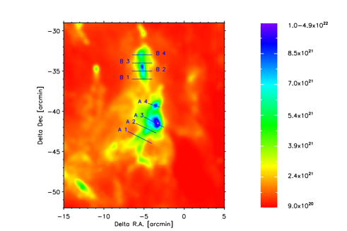
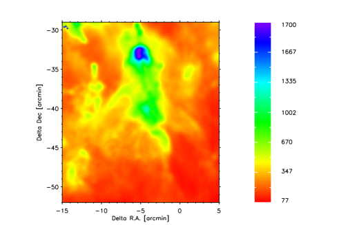
Figure 5: Upper left: Composite image (LABOCA 870 $\mu$m, Spitzer 3.6 and 8.0 $\mu$m) of the giant pillar in the Southern Pillars region (box ‘b’ in Fig. 1 and 2). Temperature map (upper right), Column density map, expressed in ${\rm cm^{-2}}$ (lower left) and Far-ultraviolet (FUV) flux $G_{0}$ (in units of the Habing field) (lower right) of the enlargement of the region. The solid lines highlight the cut lines of the prominent pillars for which temperature and column density are shown in Figure 6.

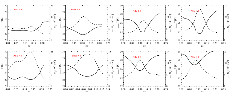
Figure 6: The plots show the temperature and column density profiles among the cuts (from left to the right, i.e. in East to West direction) of the prominent pillars highlighted in Figure 5. The solid lines represent the temperature profiles and dashed lines the column density.

Integrating our column density map over the spatial extent of the entire “giant pillar” (i.e. including both, Pillar A and Pillar B), we derive a total mass of $\approx 9350\,M_{\odot}$ for the pillar structure.

The density structure of the pillars has been also predicted by theoretical studies, e.g. by Gritschneder et al. (2010); Tremblin et al. (2012). In the simulations of Gritschneder et al. (2010) Mach 5, after 500 kyr the ionisation leads the creation of few big pillars. The most prominent pillar created by Gritschneder et al. (2010) has a size of 0.4 pc $\times$ 0.8 pc, with column density up to $1.3\times 10^{22}\leavevmode\nobreak\ {\rm cm^{-2}}$. In Tremblin et al. (2012) the formation of a slightly bigger 1 parsec long pillar takes place in the Mach 1 simulation between 200 kyr and 700 kyr. In particular their non-turbulent simulation was based on the high curvature curvature of the dense shell which leads to pillars.

The sizes of the pillars predicted by both, Gritschneder et al. (2010) and Tremblin et al. (2012), are between four and two times smaller compared to the extensions of Pillar A and Pillar B. In the simulation of Tremblin et al. (2012) it is interesting to notice that the pillar has two dense heads separated by 0.2 pc. This might explain the double peak in the temperature and density profile found in Pillar A. The column density predicted by Gritschneder et al. (2010) is in good agreement with the profile of Pillar B.

4.3 The cloud around the Treasure Chest Cluster

In the Southern Pillars region, the Treasure Chest Cluster is the largest and most prominent embedded star cluster. It is partly embedded in a dense cloud structure and is thought to be very young, with an estimated aged of less than 1 Myr (e.g. Smith et al. 2005; Preibisch et al. 2011d). The brightest and most massive cluster member is the star CPD $-59\degr\,2661$ (= MJ 632), for which a spectral type of B1Ve is listed in the SIMBAD database. In the near-infrared image (Figure 7), the cluster is surrounded by an arc of diffuse nebulosity, which seems to represent the edge of a small cavity that opens to the south-west. About $30^{\prime\prime}$ north-east of the Treasure Chest Cluster, and clearly outside this cavity, another bright star, Hen 3-485 (= MJ 640, spectral type Bep) is seen.

Our temperature, column density, and FUV intensity maps of the cloud around the cluster show a very interesting morphology, even if the structures are not well resolved. The comparison of the near-infrared image with our Herschel maps shows that the Treasure Chest Cluster is situated near the head of a pillar-like cloud. Our column density map shows that the cluster is clearly offset from the density peak ($2.3\times 10^{22}\,{\rm cm^{\rm-2}}$) of the pillar. The map also reveals a “kidney”-shaped column density depression near the location of the cluster. Our temperature map shows colder gas ($T\approx 25$ K) near the column density peak, and considerably warmer gas ($T\approx 32$ K) at the position and to the south-west of the cluster, as expected due to the local heating of the dust and gas in the cavity by the cluster stars. These results support our interpretation that the cluster is located in a small cavity at the western edge of the pillar, which is open in the south-western direction.

The star Hen 3-485 is seen (in projection) almost exactly at the column density peak of the cloud. However, its optical brightness and the moderate redenning (the observed color of $B-V=0.7$ suggest a visual extinction of $A_{V}\la 3$ mag) show that it is most likely located in front of the pillar.

Our map of the FUV intensity shows a clear peak just between the two B-stars, coinciding well with the arc of reflection nebulosity in the near-infrared image.

From our column density map we derive a total mass of $\approx 780\,M_{\odot}$ for the pillar-like cloud associated to the Treasure Chest Cluster.

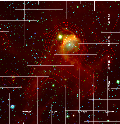
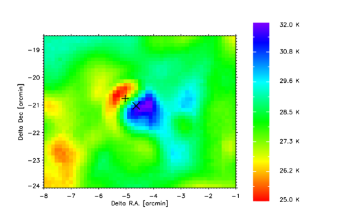
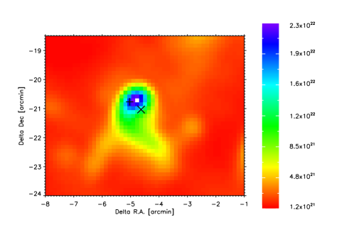
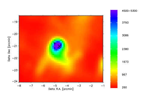
Figure 7: Upper panel: Composite image of the Treasure Chest Cluster (box ‘c’ in Fig. 1 and 2): HAWK-I $J$-band image in blue, HAWK-I $K_{s}$-band image in green, IRAC3 image in red, and the (red) contours of the LABOCA map. In the following panels are shown the temperature (upper right), column density maps (lower left) and Far-ultraviolet (FUV) flux $G_{0}$ (lower right). The column density map is expressed in ${\rm cm^{-2}}$, while the FUV in units of the Habing field. The black ‘X’ represents the position of the Treasure Chest Cluster, while the black cross the position of the star Hen 3-485.

5 Detection of a “wave”-like pattern

In the region between the central parts of the Carina Nebula and the Gum 31 region, in the northern part of our Herschel maps, our column density map reveals an interesting pattern of quite regularly spaced “waves” (see also Figure 2 and 3 of Paper I). It consists of a pattern of parallel lines (see Figure 8) running towards the north-eastern direction. The wavelength of this pattern is $\approx 14$.$7^{\prime}$, corresponding to 9.8 pc. The column density varies from $\sim 1.8\times 10^{22}\,{\rm cm^{\rm-2}}$ at the maxima to $<\,9.0\,\times 10^{20}\,{\rm cm^{\rm-2}}$ at the minima.

We first checked whether such a “wave”-like pattern can be an effect of the observation mode of Herschel. The observations are performed with two scanning directions which are later combined into the final map. The first scan direction is at 8^∘ and the second one is at 100^∘, both from West to North direction. The “wave”-like pattern is found instead at 40^∘ from the West to North direction, which does not correspond to the scan direction. We also created a final image from each scan direction and the “wave”-like pattern is present in both of them. For this reason we exclude that this is an observational effect.

One possible explanation for this pattern is that we see waves at the surface of the molecular cloud, similar to the pattern discovered in the Orion Nebula by Berné et al. (2010).

In the case of the Orion Nebula, the waves have been explained by a Kelvin-Helmholtz instability that arises during the expansion of the nebula as the gas heated and ionized by massive stars is blown over pre-existing molecular clouds that are located a few parsecs away from the center of the cluster, where the young massive stars are concentrated.

The situation in the Carina Nebula is similar: The feedback from the numerous massive stars in the central regions of the Carina Nebula drives a bipolar bubble (Smith et al. 2000).

The location of the observed wave pattern agrees roughly with the northern part of this bubble system. The waves are seen at a projected distance of $\sim 6-15$ pc from the massive stars in Tr 16 and Tr 14. For a comparison to the Orion Nebula case, this larger distance may be easily compensated by the much larger number of massive stars in the Carina Nebula and the correspondingly higher level of stellar feedback. Therefore, the density and velocity of the hot plasma that is thought to cause the wave pattern in the Orion Nebula may well be of a similar order of magnitude as in the pattern we see in the Carina Nebula.

Some information about the outflowing material can be obtained from the Chandra X-ray survey in the context of the Chandra Carina Complex Project (CCCP) (see Townsley et al. 2011b). A detailed analysis of the diffuse X-ray emission, which traces the hot plasma, is given in Townsley et al. (2011a).

The largest part of the wave pattern revealed by Herschel lies just outside the area covered by the Chandra X-ray map. At the north-eastern edge of the Chandra X-ray map, which touches the south-western edge of the wave pattern revealed by Herschel, the dominant plasma components have temperatures ranging from 0.14–0.17 keV to 0.25–0.27 keV.

The ROSAT image, that covers a larger field-of-view than the Chandra map, shows that the amplitude of the diffuse X-ray emission in the area of the wave pattern is rather weak. This suggests that the hot plasma in this region is not confined, but streaming outwards.

The most remarkable difference to the waves in the Orion Nebula is the substantially longer wavelength of the wave pattern in the Carina Nebula, $\sim 10$ pc rather than $\sim 0.1$ pc. According to the models of Berné et al. (2010), this longer wavelength suggests that a plasma of density $\sim 1\,{\rm cm}^{-3}$ with a flow velocity of $\sim 100$ km/s could be causing the instability. Such values appear quite possible in the case of the Carina Nebula superbubble.

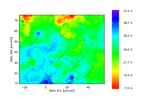
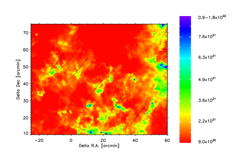
Figure 8: Temperature (left) and column density, expressed in ${\rm cm^{-2}}$, (right) map of the north-eastern part of the Carina Nebula Complex (box ‘d’ in Fig. 1 and 2). The dashed lines represent a “wave pattern” which seems to connect the two main regions of the complex.

6 Discussion

6.1 Comparison of dense and diffuse gas

In Fig. 9 we compare the Herschel  $160\,\mu$m map to the LABOCA $870\,\mu$m map presented in Preibisch et al. (2011d). This combination has the advantage that the angular resolution of the Herschel  $160\,\mu$m map ($\approx 12^{\prime\prime}-16^{\prime\prime}$) matches the angular resolution of the LABOCA map ($18^{\prime\prime}$) quite well. The differences in these maps are thus not due to the difference in angular resolution (as would be the case for the other Herschel maps) but rather trace the differences in the spatial distributions of the very cold gas and the somewhat warmer gas.

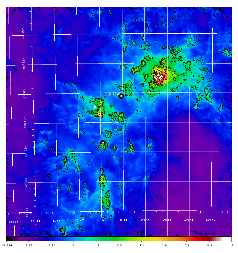
Figure 9: Herschel  $160\,\mu$m map (in Jy/px) with the LABOCA $870\,\mu$m contours overlaid at 0.08, 0.16, 0.32, 0.64, 1.28, 2.56 Jy/beam. Highlighted is the position of $\eta$ Car.

In most clouds, the cold gas (traced by the sub-mm emission) is considerably more spatially concentrated than the warmer gas (traced in the Herschel  $160\,\mu$m map). The most prominent example is the dense cloud west of Tr 14, in which the cold dense cloud center is surrounded by a much more extended halo of widespread warmer gas.

However, in many of the pillars we find a very different situation. Most pillars that are seen $\sim 15^{\prime}-20^{\prime}$ to the south-east of $\eta$ Car, are not surrounded by significant amounts of extended warm gas. The spatial extent of the warmer gas matches that of the cold gas quite well.

The pillars at the southern periphery (more than $\sim 20^{\prime}$ south of $\eta$ Car) show filaments of warmer gas at their base that seems to stream away from the densest parts of these clouds in the direction opposite to the pillar head, just as expected in the scenario of cloud dispersal by ionizing irradiation.

A particularly interesting difference in the spatial configuration of the cold gas versus the warmer gas is displayed by the cloud structure $\sim 5^{\prime}$ - $10^{\prime}$ to the south and south-east of $\eta$ Car (that constitutes the “left wing” of the V-shaped dark cloud). Here, the cold gas is highly concentrated in two distinct compact clouds (labeled as ’A’ and ’B’ in Fig. 9), which have a gap (with a width of about $3^{\prime}$) between them, just at the position that is closest (in projection) to $\eta$ Car. In a remarkable contrast, the configuration of the warmer gas resembles just a continuous elongated distribution, with no indication of any gap at this position. This implies that there is a considerable amount of warmer gas in the region between these two clumps of cold gas.

6.2 Dust vs. molecular gas mass estimates for individual clumps

The area covered by our Herschel maps includes 14 of the C¹⁸O clumps detected and characterized in the study of Yonekura et al. (2005). Compact clouds are seen in our Herschel maps at the locations of all of these clumps with exception of C¹⁸O clump number 10.

In order to derive clump mass estimates from their FIR emission, we integrated over boxes centered at the cloud positions as seen in our Herschel maps that correspond to the reported positions of the C¹⁸O clumps of Yonekura et al. (2005). Our box sizes were chosen to be as similar as possible to the sizes given by Yonekura et al. (2005) (details in Table 2). Eight of the C¹⁸O clumps are also located in the field of view of our previous LABOCA observations (Preibisch et al. 2011c), from which we already estimated clump masses based on their sub-mm fluxes. In Table 2 we summarize the total, gas + dust, clump masses and temperatures computed using the different methods.

This comparison shows that the masses computed from the our Herschel maps agree generally quite well to the previous estimates based on the sub-mm fluxes. However, the masses based on FIR and sub-mm data are always about $2-4$ times lower than the masses estimated by Yonekura et al. (2005) from their C¹⁸O data.

There are several possible explanations for this discrepancy. One major issue are the extrapolation factors used relating the measured dust or CO molecule emission to the total gas + dust mass. It is well known that the gas-to-dust ratio, for which we assumed the canonical value of 100, is uncertain by (at least) about a factor of 2. Concerning the masses derived from CO, it is known that the fractional abundance of carbon-monoxide may not be constant but depend on the cloud density; thus, the factor used to extrapolate the CO mass to the total mass can easily vary by factors of 2–3 (see, e.g., discussion in Goldsmith et al. 2008).

We also find small, but systematic differences in the derived cloud temperatures. In most clumps, the dust temperature we derive from our Herschel maps is a few Kelvin higher than the CO gas temperatures derived by 2. This is probably related to the fact to both temperatures represent averages over (i) the corresponding beam area and (ii) along the entire line-of-sight though the clumps. Since real clumps are not spatially isothermal but have some kind of (unresolved) density and temperature structure, the different biases of the different observations result in these different temperature values.

We finally note that the Herschel maps show many more dense cold dusty clouds, which remained undetected in the C¹⁸O maps.

Table 2: Mass and temperature derived for the C¹⁸O clumps from Yonekura et al. (2005).

Clump	Coordinates		Size	MFIR	MSub-mm	M${}_{\rm C^{18}O}$	T	T
number	$\alpha_{\rm J2000}$	$\delta_{\rm J2000}$	[′]	[M⊙]	[M⊙]	[M⊙]	[K]	[K]
1	$10^{\rm h}\,34^{\rm m}\,23^{\rm s}$	$-58\degr\,47^{\prime}\,00^{\prime\prime}$	6$\times$6	420	–	1785	18-21	16
2	$10^{\rm h}\,36^{\rm m}\,43^{\rm s}$	$-58\degr\,32^{\prime}\,39^{\prime\prime}$	7$\times$12	1232	–	3910	20-26	15
4	$10^{\rm h}\,37^{\rm m}\,41^{\rm s}$	$-58\degr\,26^{\prime}\,33^{\prime\prime}$	4$\times$7	464	–	850	21-26	20
5	$10^{\rm h}\,38^{\rm m}\,33^{\rm s}$	$-58\degr\,19^{\prime}\,15^{\prime\prime}$	7$\times$7	269	–	5185	25-29	28
6	$10^{\rm h}\,38^{\rm m}\,09^{\rm s}$	$-58\degr\,45^{\prime}\,58^{\prime\prime}$	12$\times$7	1212	–	3145	23-28	26
7	$10^{\rm h}\,37^{\rm m}\,53^{\rm s}$	$-58\degr\,55^{\prime}\,37^{\prime\prime}$	7$\times$8	885	–	1360	20-21	17
8	$10^{\rm h}\,41^{\rm m}\,14^{\rm s}$	$-59\degr\,40^{\prime}\,50^{\prime\prime}$	8$\times$7	2391	829	3145	22-26	24
9	$10^{\rm h}\,42^{\rm m}\,38^{\rm s}$	$-59\degr\,26^{\prime}\,49^{\prime\prime}$	5$\times$5	476	593	1190	23-28	21
11	$10^{\rm h}\,43^{\rm m}\,56^{\rm s}$	$-59\degr\,24^{\prime}\,21^{\prime\prime}$	5$\times$5	610	312	1190	23-25	22
12	$10^{\rm h}\,45^{\rm m}\,15^{\rm s}$	$-59\degr\,48^{\prime}\,22^{\prime\prime}$	6$\times$5	882	1095	2210	23-26	20
13	$10^{\rm h}\,45^{\rm m}\,48^{\rm s}$	$-60\degr\,18^{\prime}\,09^{\prime\prime}$	7$\times$9	1748	1212	3570	22-27	20
14	$10^{\rm h}\,48^{\rm m}\,14^{\rm s}$	$-59\degr\,58^{\prime}\,48^{\prime\prime}$	3$\times$3	161	85	382	23-26	9
15	$10^{\rm h}\,47^{\rm m}\,50^{\rm s}$	$-60\degr\,26^{\prime}\,15^{\prime\prime}$	4$\times$5	353	453	1700	20-23	19

6.3 Cloud mass budgets based on different tracers

In Table 3 we summarize the integrated cloud masses for different parts of the CNC derived from different tracers. The masses derived in this paper via fitting of the FIR spectral energy distribution, and in Preibisch et al. (2011c) from sub-mm fluxes, are based on dust as a mass tracer. The study of Yonekura et al. (2005) gives mass estimates derived from different CO isotopologues, and is thus based on gas tracers.

Considering the total cloud complex, we find rather good agreement between the different mass estimates for specific column density thresholds. Our Herschel based cloud mass estimate for an column density threshold corresponding to $A_{V}>1$ is well consistent with the mass estimate based on ¹²CO. This is in good agreement with the standard idea that molecules exist inside the shielded regions of dark clouds (Goldsmith et al. 2008). The thresholds in $A_{V}$ of 0.9 and 7.3 have been chosen as in Lada et al. (2012).

Our previous cloud mass estimate based on the LABOCA sub-mm flux (Preibisch et al. 2011c) agrees well with the mass estimate based on ¹³CO. This fits with the assumption that the LABOCA sub-mm map traces only dense clouds and that ¹³CO is a tracer of relatively dense gas.

The total mass of all individual clumps detected in our LABOCA sub-mm map (as determined by Pekruhl et al. 2013) is between the cloud mass estimates based on ¹³CO and C¹⁸O, in good agreement with the idea that C¹⁸O traces denser gas than ¹³CO.

6.4 The strength of the radiative feedback

As mentioned above, the cloud surfaces in the CNC are strongly irradiated: we find $G_{0}$ values generally between $\sim 1000$ and up to $\approx 10\,000$. These numbers provide important quantitative information on the level of the radiative feedback from the massive stars on the clouds.

To put these numbers in context, we refer to the compilations in Brooks et al. (2003) (Tab. 3) and Schneider & Brooks (2004) (Tab. 2), where values of the FUV field strengths in photo-dissociation regions (PDRs) in different star forming regions are listed. This comparison shows that the FUV field strength at the cloud surfaces in the CNC is very similar to that measured for PDRs in the 30 Dor cluster, which is generally considered as the most nearby extragalactic starburst system. This result supports the idea that the level of massive star feedback in the CNC is similar to that found in starburst systems.

The comparison also shows that, sometimes, even higher values of the FUV field strength are found at specific locations in much less massive star forming regions. For example, in the PDR in the Orion KL region, $G_{0}$ values up to $10^{4}-10^{5}$ have been determined (see references in Schneider & Brooks 2004). Such high local values are, however, only found in clouds located very close (less than 1 parsec) to individual high-mass stars, i.e. restricted to very small cloud surface areas. No such extremely high irradiation values are seen in the CNC, because the clouds are generally at least a few parsecs away from the massive stars. This is probably a consequence of the fact that many of the massive stars in the CNC are several Myr old and have thus already dispersed the clouds in their immediate surroundings (by their high level of feedback).

Despite the fact that some lower-mass star forming regions show peaks of FUV irradiation that can locally exceed the levels we see in the CNC, the total amount of hard radiation (and thus the total power available for feedback) is much higher in the CNC.

The high level of the FUV irradiation may also affect the circumstellar matter around the young stellar objects in the CNC. The irradiation causes increased external heating and photoevaporation of the circumstellar disks and can disperse the disks within a few Myr. This process has been directly observed in the so-called “proplyds” near the most massive stars in the Orion Nebula Cluster (O’dell et al. 1993; Bally et al. 2000; Ricci et al. 2008) and has been theoretically investigated by numerical simulations (e.g., Richling & Yorke 2000; Adams et al. 2004; Clarke 2007)

Using near-infrared excesses as an indicator of circumstellar disks, our previous studies of X-ray selected young stars in the different populations in the CNC actually showed that the infrared excess fractions for the clusters in the CNC are lower than those typical for stellar clusters of similar age with lower levels of irradiation (Preibisch et al. 2011c). This is consistent with the idea that the high level of massive star feedback in the CNC causes faster disk dispersal. Similar indications have been found in other high-mass star forming regions, where the disk fractions were also found to be lower close to high mass stars (e.g. Fang et al. 2012; Roccatagliata et al. 2011).

6.5 On the relative importance of massive star feedback and primordial turbulence

A fundamental question of star formation theory is whether the structure of the clouds in a star forming region is dominated by primordial turbulence or by massive star feedback.

The recent study of Schneider et al. (2010) analyzed Herschel observations of the Rosette molecular clouds and suggested that “there is no fundamental difference in the density structure of low- and high-mass star-forming regions”. They argue that the primordial turbulent structure built up during the formation of the cloud, rather than the feedback from massive stars, is determining the course of the star formation process in this region. The current star formation process is concentrated in the most massive filaments that were created by turbulent gas motions. The star-formation can be triggered in the direct interaction zone between the HII-region and the molecular cloud but probably not deep into the cloud on a size scale of tens of parsecs.

It is interesting to compare the Rosette molecular cloud to the CNC. The Rosette cloud has a similar, only slightly lower total cloud mass than the CNC, and also harbors a rather large population of OB stars. However (as already pointed out by Schneider & Brooks 2004; Schneider et al. 1998), the Rosette Molecular Cloud is exposed to a much (about 10 times) weaker UV field than what we find in the Carina Nebula. This order-of-magnitude difference in the level of the radiative feedback may explain the differences in the cloud structure of these two complexes. In strong contrast to the predominantly filamentary cloud structure of the Rosette region, most clouds in the CNC show pillar-like shapes. Our Herschel maps reveal (as previously suggested on the basis of the Spitzer data; Smith et al. 2010) the systematic and ordered shape and orientation of these numerous pillars, that point towards clusters of high-mass stars. As discussed in Gaczkowski et al. (2013), the current star formation activity in the CNC is largely concentrated to these pillars. These results clearly suggest that the cloud structure and the star formation activity in the CNC is dominated by stellar feedback, rather than random turbulence.

A strong feedback similar to the situation in the CNC has been found in Herschel study of the RCW36 bipolar nebula in Vela C by Minier et al. (2013).

6.6 Total FIR luminosity

From our map of the FIR intensity we also computed the total FIR luminosity in the $60-200$ $\mu$m wavelength range, $L_{\rm FIR,tot}$ by integrating over a $2.3\degr\times 2.3\degr$ region covering the entire CNC. We find a value of $L_{\rm FIR,tot}=(1.7\pm 0.3)\times 10^{7}\,L_{\odot}$.

This value is somewhat larger than the total infrared luminosity of $1.2\times 10^{7}\,L_{\odot}$ measured by Smith & Brooks (2007) from IRAS and MSX data, but this difference can be explained by the slightly smaller area used in the study of Smith & Brooks (2007), that excluded the Gum 31 region (see their Fig. 1c).

It is interesting to compare this total FIR luminosity to the total luminosity of the known massive stellar population in the CNC, as derived by Smith (2006): Our total FIR luminosity is smaller than the total stellar bolometric luminosity of $2.5\times 10^{7}\,L_{\odot}$, but 70% larger than the total stellar FUV luminosity of $1.0\times 10^{7}\,L_{\odot}$. The most likely explanation for this apparent discrepancy of the total FIR and total FUV luminosity is that the current census of massive stars in the CNC is still incomplete. Direct support for this assumption comes from the study of Povich et al. (2011), who could identify 94 new candidate OB stars (with $L_{\rm bol}\geq 10^{4}\,L_{\odot}$) among X-ray selected infrared sources in the Carina Nebula. They found that the true number of OB stars in the CNC is probably about 50%, and perhaps up to 100%, larger than the currently identified OB population. This incompleteness results from the lack of sufficiently deep wide-field spectroscopic surveys, that left a significant number of OB stars yet unidentified.

Taking this incompleteness into account, the extrapolated total stellar FUV luminosity would match the total FIR luminosity we derived quite well.

6.7 The Carina Nebula as a link between local and extragalactic star formation

Lada et al. (2012) collected observational data for numerous Galactic star forming regions and external galaxies and found a well-defined scaling relation between the star formation rates and molecular cloud masses above certain column density thresholds. They expressed the star formation scaling law for these clouds as

$${\rm SFR}=4.6\times 10^{-8}\,f_{\rm DG}\,M_{G}(M_{\sun})\,M_{\sun}\,{\rm yr}^{-1}$$ (3)

where $M_{G}$ is molecular mass measured at a particular extinction threshold and corrected for the presence of helium and $f_{\rm DG}$ is the fraction of dense gas.

They suggest that this fundamental relation holds over a span of mass covering nearly nine orders of magnitude. Although the exact physical meaning of certain density threshold values is not clear (see discussion in Burkert & Hartmann 2012), this empirical relation provides an interesting opportunity to compare different star formation regions. In the compilation of observational data of Lada et al. (2012), there is a gap of about four orders of magnitude (in cloud mass) between the local Galactic clouds and the external galaxies. The CNC is ideally suited to bridge this gap and to connect Galactic and extragalactic regions in this investigation.

The cloud masses for the CNC determined with different tracers have been summarized above. For the extinction thresholds of $A_{K}>0.1$ mag and $A_{K}>0.8$ mag, as used in the study of Lada et al. (2012), we find total cloud masses of $\sim 610\,000\,M_{\odot}$ and $\sim 23\,000\,M_{\odot}$ from our Herschel data of the entire CNC.

Taking into account the systematic calibration uncertainties of the Herschel fluxes as well as uncertainty of the exact boundaries of the CNC, we estimate an uncertainty of 30% for the total cloud mass.

For the star formation rate in the CNC, several recent determinations are available. Povich et al. (2011) analyzed a Spitzer-selected sample of YSOs in the central 1.4 square-degrees of the Carina Nebula. From this they derived a lower limit of $\dot{M}>0.008\,M_{\odot}\,{\rm yr}^{-1}$ for the star formation rate averaged over the past $\sim 2$ Myr. From an analysis of the optically visible populations of stars in the Carina Nebula, they derived an average star formation rate over the past 5 Myr of $\dot{M}\approx 0.010-0.017\,M_{\odot}\,{\rm yr}^{-1}$. In our analysis of the YSO detected as point-like sources in our Herschel data of the entire CNC (i.e., including the Gum 31 region) we estimated a star formation rate $0.017\,M_{\odot}\,{\rm yr}^{-1}$ (Gaczkowski et al. 2013), which is an average over the last few $10^{5}$ years. The error associated to the star formation rate is about 50% (details in Gaczkowski et al. 2013). Taking the smaller area covered by the Spitzer studies into account, it can be shown (see Gaczkowski et al. 2013, for details) that our Herschel-based star formation rate estimate is in good agreement with the rates derived by Povich et al. (2011).

In Figure 10 we add our data for the CNC to the star formation rate versus cloud mass diagram from Lada et al. (2012). Since the cloud mass as well as star formation rate of the CNC are larger than in all other Galactic regions shown in the original plot, the CNC adds an important new data point in the gap between the other Galactic regions and the external galaxies.

Considering the total cloud mass above the $A_{K}>0.1$ mag threshold, the data point for the CNC appears to follow the general relation. The cloud mass above the $A_{K}>0.8$ mag threshold, however, appears to be considerably lower than the expectation according to the general relation. This implies that the star formation rate per unit mass in dense clouds is higher in the CNC compared to the other regions. In other words, the star formation process seems to be exceptionally efficient in the CNC.

Dividing the total mass in dense clouds of $23\,000\,M_{\odot}$ by the star formation rate of $0.017\,M_{\odot}\,{\rm yr}^{-1}$ yields a characteristic timescale of 1.3 Myr. If one would simply assume that the total mass of the currently present dense clouds will be turned into stars at a temporally constant rate, this process would last 1.3 Myr. Considering the clearly established fact that star formation in the CNC is going on since (at least) about 5 Myr (as witnessed by the large populations of young stars in the optically visible populations), this would imply that the star formation process in the CNC will soon come to its close and the observed dense clouds are the last remaining parts of the original clouds.

However, we believe that it is probably not correct to think in terms of a fixed amount of dense clouds that just turns into stars over time. Rather, a large fraction of the dense clouds that are present today, may have just recently been actively created by the feedback of the massive stars.

Several studies of the youngest stellar populations in the CNC came to the conclusion that the currently ongoing star formation process is, to a large degree, spatially restricted to the edges and surfaces of irradiated clouds, e.g. the tips of the numerous pillars (Smith et al. 2010; Ohlendorf et al. 2012; Gaczkowski et al. 2013). This suggests a causal connection between the star formation process and local cloud compression. The ongoing feedback continues to compress (moderately dense) clouds and thus can create new dense cloud structures that, once they get gravitationally unstable, will collapse and form stars.

In this dynamic picture, where dense cloud structures are constantly created, the ratio of dense cloud mass versus the star formation rate is naturally lower than in the case of clouds that do not experience significant levels of compression from massive star feedback. This may explain the position of the CNC in this plot. The CNC shows the largest deviation from the SFR versus cloud mass relation than all other plotted Galactic star forming regions because the level of massive star feedback is particularly high.

It is interesting to note some of the “(ultra-) luminous infrared galaxies” show deviations in the same sense, i.e. SFRs that are higher than expected form the dense cloud mass. This is consistent with the idea that a high level of feedback is increasing the efficiency of star formation.

Since numerous galactic star forming regions have now been observed by Herschel, the analysis of these data will soon show whether similarly large star forming complexes with comparable levels of feedback do also show a similar behavior between cloud mass and star formation rate.

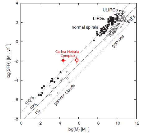
Figure 10: Plot adopted from Fig.2 in Lada et al. (2012). The red points represent the position of the star formation rate and the total mass of the entire Carina Nebula Complex. The error in the $\log\,(M)$ is 0.1 (i.e. $\sim$30% of the total mass), and the error in $\log\,(SFR)$ is 0.2 (i.e. $\sim$50% of the star formation rate). The empty points represent the cloud mass computed over an extinction threshold of A${}_{K}>0.1$ and the filled point over A${}_{K}>0.8$ (as in Lada et al. 2012). three parallel lines correspond to $f_{\rm DG}=$ 1.0, 0.1, and 0.01 (defined in Equation 3) from left to right, respectively.

Table 3: Cloud mass budget (in M_⊙) using different methods.

Trace		Area		Ref.
		2.3${}^{\circ}\times$2.3∘	1.2${}^{\circ}\times$1.2∘
Total NIR-Radio SED		900 000		2
FIR
	SED - A${}_{\rm V}>0.9$	609 765	147 259	1
	SED - A${}_{\rm V}>1.0$	421 704	128 220	1
	SED - A${}_{\rm V}>7.3$	22 903	8 115	1
Sub-mm/mm
	LABOCA		60 000	3
	LABOCA (Clumps)		42 000	4
	12CO	346 000	141 000	5
	13CO	132 000	63 000	5
	C18O	57 800	22 000	5

(1) This work; (2) Preibisch et al. (2011d); (3) Preibisch et al. (2012) (Paper I); (4) Pekruhl et al. (2013); (5) Yonekura et al. (2005).

7 Conclusions and Summary

Our wide-field Herschel SPIRE and PACS maps allowed us to determine the temperatures, surface densities, and the local strength of the FUV irradiation for all cloud structures over the entire spatial extent ($\approx 125$ pc in diameter) of the Carina Nebula complex at a spatial resolution of $\la 0.4$ pc for the first time. The main results and conclusions of our study can be summarized as follows:

1. The global temperature structure of the clouds in the CNC is clearly dominated by the radiative feedback from the numerous massive stars.

2. We present detailed temperature, column density, and FUV intensity maps of particularly interesting small-scale cloud structures in the CNC.

3. The comparison of the Herschel FIR maps to a sub-mm map of the CNC shows that the cold gas, traced by the sub-mm emission, is more spatially concentrated than the warmer gas, traced by Herschel.

4. Considering the masses of individual clumps determined from their FIR dust emission, we find that previous mass estimates that were obtained from CO molecular line observations yielded systematically (by factors of $\sim 2-4$) larger values. This difference probably results from uncertainties in the absolute calibration of the different mass tracers and from the different biases (and beam sizes) of the observations.

5. We investigate the total cloud mass budget in the CNC at different column density thresholds and find that the different tracers (dust and CO) yield consistent total masses for the moderately dense gas (as traced by ¹²CO) and the dense gas (as traced by ¹³CO and C¹⁸O).

6. The intensity of the FUV irradiation at most cloud surfaces in the CNC is at least about 1000 times stronger than the galactic average value (the so-called Habing field). At some locations, e.g. at the surface of the massive cloud to the west of the stellar cluster Tr 14, the FUV irradiation is more than 10 000 times the Habing field.

7. In a region north of the Carina Nebula, we discover a “wave”-like pattern in the column-density map. This pattern may be related to a flow of hot gas streaming out of the northern part of the bipolar superbubble.

8. We compare the ratio between the total cloud mass and the star formation rate in the CNC to the sample of Galactic and extragalactic star forming regions originally presented by Lada et al. (2012). This shows that the CNC seems to form stars with a higher efficiency than other, typically lower-mass, Galactic star forming regions. We suggest that this is a consequence of the particularly strong radiative feedback in the CNC. The compression of the clouds actively and continuously creates dense clouds out of lower density diffuse clouds. In this way, the total amount of dense clouds is continuously replenished.

9. We present the first detailed FIR mapping and mass estimates for two cloud complexes seen at the edges of our Herschel maps, which are molecular clouds in the Galactic background at distances between 7 and 9 kpc.

Appendix A Cloud complexes at the edges of the Herschel maps

Besides the clouds associated to the Carina Nebula and the Gum 31 region, our Herschel maps also show several cloud structures at the periphery of the field of view. The two most prominent peripheral cloud complexes are seen near the south-eastern edge and the western edge of our map. Since no detailed FIR observations of these clouds seem to be available so far in the literature, we briefly describe the FIR morphology of these cloud complexes as revealed by our Herschel maps and discuss identifications with observations at other wavelengths.

A.1 The G$289.0-0.3$ cloud complex

A cloud complex extending over about $35^{\prime}\times 35^{\prime}$ is seen around the position $(\alpha_{\rm J2000},\,\delta_{\rm J2000})\,=\,(10^{\rm h}\,56^{\rm m}\,30^{\rm s},\,-60\degr\,06^{\prime}\,00^{\prime\prime})$ , near the south-eastern edge of our SPIRE maps. Optical images of this region show numerous field stars, but no prominent cloud features. The cloud complex we see in the Herschel maps is related to the radio-detected molecular cloud G289.0-0.3 described by Russeil & Castets (2004). With a radial velocity of $v_{\rm rad}=+27.5$ km/s, this cloud complex seems to be clearly unrelated to the Carina Nebula cloud complex (which has $v_{\rm rad}\approx-26$ km/s).

Besides the diffuse cloud emission, our Herschel maps revealed 52 individual point-like sources, the positions and fluxes of which are given in Gaczkowski et al. (2013). Several of these can be identified with IRAS or MSX point-sources, some of which are marked in Fig. 11. The brightest compact Herschel source in this area can be identified with the giant H II region PMN J1056-6005, which was detected in the Parkes-MIT-NRAO 4850 MHz survey (Griffith & Wright 1993), and seems to be identical to the H II region GAL 289.06-00.36 listed in Caswell & Haynes (1987). Cersosimo et al. (2009) detected emission in the H166$\alpha$ radio recombination line from this region and determined a distance of $D=7.1\pm 0.3$ kpc. We note that this distance value is consistent with the prediction of the velocimetric model of the Galaxy by Vallée (2008) for the galactic longitude and the measured radial velocity of this molecular cloud complex.

At the southern tip of the cloud complex, the Be star CPD–59 2854 (= IRAS 10538-5958) is seen as a bright compact far-infrared source. In the northern part of this complex, one of the bright Herschel point-like sources is the extended 2MASS source 2MASX J10543287-5939178, which is listed as a Galaxy in the SIMBAD catalog, but may in fact be an ultra-compact H II region (Bronfman et al. 1996).

Since this cloud complex is located near the edge of our Herschel maps, and a considerable fraction is only covered by the SPIRE maps, but not by PACS, we cannot provide a complete characterization of this cloud complex. In our temperature map, the dust temperatures in these clouds ranges from about 18 K to about 25 K. Integrating our column density map (see Section3) over a $16^{\prime}\times 19^{\prime}$ area, covering that part of the cloud complex that is observed by PACS and SPIRE, we obtain a total mass of $65\,000\,M_{\sun}$. Due to the incomplete spatial coverage, this is clearly a lower limit to the total cloud mass of this complex.

This rather high cloud mass and the remarkably high number of detected point-like Herschel sources clearly show that this cloud complex is a region of active massive star formation that is worth to be studied in more detail.

A.2 The G$286.4-1.3$ cloud complex

Near the western edge of our PACS maps, a cloud complex extending over about $16^{\prime}\times 19^{\prime}$ is seen around the position $(\alpha_{\rm J2000},\,\delta_{\rm J2000})\,=\,(10^{\rm h}\,34^{\rm m}\,00^{\rm s},\,-59\degr\,47^{\prime}\,00^{\prime\prime})$. Optical images of this region show several dark clouds.

The cloud complex seems to be related to the radio-detected molecular cloud G286.4-1.3 discussed by Russeil & Castets (2004). The radial velocity of $v_{\rm rad}=+39.9$ km/s is clearly distinct from that of the Carina Nebula cloud complex ($v_{\rm rad}\approx-26$ km/s). We note that no CO emission from these clouds was detected in the survey of Yonekura et al. (2005).

Besides the diffuse cloud emission, our Herschel maps revealed 15 individual point-like sources in these clouds, the positions and fluxes of which are given in Gaczkowski et al. (2013). The brightest emission peak in this complex can be identified with the ultra-compact H II region IRAS 10320-5928 (Bronfman et al. 1996).

The southern part of the cloud complex contains the FIR source IRAS 10317-5936, which is identified with the H II region GAL 286.42-01.48 and listed as part of the star-forming complex 286.4-01.4 in Russeil (2003). It contains the two candidate massive young stellar objects 286.3938-01.3514 1 and 2 (Mottram et al. 2007). Fontani et al. (2005) determined a distance of $D=8.88$ kpc to this cloud. We note that this distance value is consistent with the prediction of the velocimetric model of the Galaxy by Vallée (2008) for the galactic longitude and the measured radial velocity of this molecular cloud complex.

In the north-western part of this complex, another accumulation of compact clouds is found, two of which can be identified with IRAS sources.

The main part, but not the full extent of this cloud complex is covered by our PACS and SPIRE maps. The dust temperatures range from about 20 K to $\ga 35$ K. Integrating our column density map yields a total mass of $\sim 93\,000\,M_{\odot}$ within a $16^{\prime}\times 19^{\prime}$ area, if we assume the above mentioned distance of 8.88 kpc. This is a strict lower limit, since our data cover only some part of the cloud complex.

This rather high cloud mass and the presence of numerous bright point-like Herschel sources (with fluxes up to $\approx 530$ Jy, corresponding to FIR luminosities of up to $\sim 25\,000\,L_{\odot}$) shows that this complex is a site of active massive star formation and certainly worth to be studied in more detail.

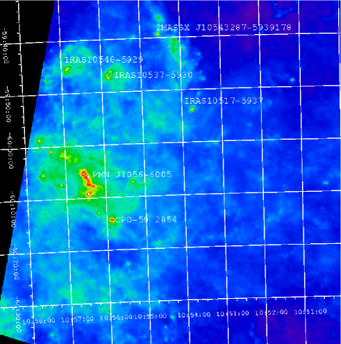
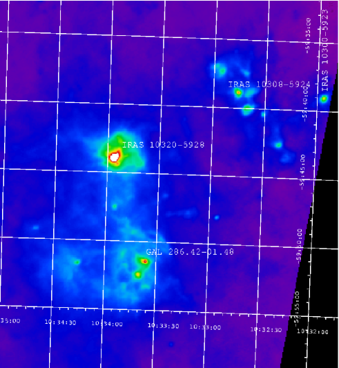
Figure 11: Right: Herschel / PACS $70\,\mu$m map of the G$286.4-1.3$ cloud complex; Left: Herschel / SPIRE $250\,\mu$m map of the G$289.0-0.3$ cloud complex.