Full-Duplex Cooperative Cognitive Radio with Transmit Imperfections

Abstract

This paper studies the cooperation between a primary system and a cognitive system in a cellular network where the cognitive base station (CBS) relays the primary signal using amplify-and-forward or decode-and-forward protocols, and in return it can transmit its own cognitive signal. While the commonly used half-duplex (HD) assumption may render the cooperation less efficient due to the two orthogonal channel phases employed, we propose that the CBS can work in a full-duplex (FD) mode to improve the system rate region. The problem of interest is to find the achievable primary-cognitive rate region by studying the cognitive rate maximization problem. For both modes, we explicitly consider the CBS transmit imperfections, which lead to the residual self-interference associated with the FD operation mode. We propose closed-form solutions or efficient algorithms to solve the problem when the related residual interference power is non-scalable or scalable with the transmit power. Furthermore, we propose a simple hybrid scheme to select the HD or FD mode based on zero-forcing criterion, and provide insights on the impact of system parameters. Numerical results illustrate significant performance improvement by using the FD mode and the hybrid scheme.

I Introduction

Recently there has been a new paradigm to improve the spectrum efficiency of a cognitive radio network by introducing active cooperation between the primary and cognitive systems [1]-[7]. As illustrated in Fig. 1, the cognitive system helps relay the traffic from the primary base station (PBS), and in return can utilize the primary spectrum for secondary use. This is of particular importance to the primary system when the primary user (PU)’s data rate or outage probability requirement cannot be satisfied by itself. Therefore both systems have strong incentive to cooperate as long as such an opportunity exists. A three-phase cooperation protocol between primary and cognitive systems termed “spectrum leasing” is proposed to exploit primary resources in time and frequency domain [3], [4]. During Phase I and II, the cognitive base station (CBS) listens and forwards the primary traffic; in the remaining Phase III, the CBS can transmit its own signal to the cognitive user (CU). Note that to avoid additional interference, in Phase II, the PBS remains idle and only the CBS transmits signals. The use of multiple-input-multiple-output (MIMO) antennas and beamforming at the CBS provides additional degree of freedom for primary-cognitive cooperation in the spatial domain [5][6][7]. In comparison to the conventional spectrum leasing, MIMO CBS requires only two phases: Phase I is the same as that in spectrum leasing while in Phase II, the relay can both forward primary signal and transmit its own signal.

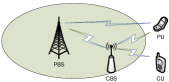
Figure 1: Cooperation between a primary system and a cognitive system

However, most existing works assume half-duplex (HD) mode for the CBS so at least two orthogonal communication phases are needed, which brings losses to throughput. As a result, the primary-cognitive cooperation is not always useful, meaning that the achievable primary rate can be even lower than that of the direct transmission. To remedy the situation, this paper investigates the potential use of full-duplex (FD) mode for the CBS, i.e., it simultaneously receives primary message, and transmits processed primary signal and its own cognitive signal on the same channel. Since overall only one channel phase is used, the FD mode is an efficient technique to enlarge the achievable rate region.

I-A Related Work

FD has attracted lots of research interests especially for relay assisted cooperative communication. Traditionally, FD is considered to be infeasible due to the practical difficulty to recover the desired signal which suffers from the self-interference from the relay output, which could be as high as 100 dB [8]. It is shown in [9] that the FD relaying in the presence of loop interference is indeed feasible and can offer higher capacity than the HD mode. Experimental results are reported in [10] that the self-interference can be sufficiently cancelled to make FD wireless communication feasible in many cases; hardware implementations in [11] show over 70% throughput gains from using the FD over the HD in realistically used cases. Since then, there have been substantial efforts on dealing with self-interference. Utilizing multiantenna techniques, [12] proposes to direct the self-interference of a DF relay in the FD mode to the least harmful spatial dimensions. The authors of [13] analyze a wide range of self-interference mitigation when the relay has multiple antenna, including natural isolation, time-domain cancellation and spatial domain suppression. The techniques apply to general protocols including amplify-and-forward (AF) and decode-and-forward (DF). The transmitter/receiver dynamic-range limitations and channel estimation error at the MIMO DF relay is considered explicitly in [14], and an FD transmission scheme is proposed to maximize a lower bound of the end-to-end achievable rate by designing transmit covariance matrix. Considering the tradeoff between residual interference in the FD mode and rate loss in the HD mode, in [15], a hybrid FD/HD relaying is proposed together with transmit power adaption to best select the most appropriate mode. Relay selection is examined in [16] in AF cooperative communication with the FD operation, and shows that the FD relaying results in a zero diversity order despite the relay selection process.

In the area of cooperative cognitive radio, there have been very few works on the use of the FD mode. It is worth mentioning that a theoretical upper-bound for the rate region was found in [17] [18][19], where the CBS employs dirty paper coding (DPC) to remove interference from the CU due to the primary signal. However, DPC requires non-causal information about the primary message at the CBS, in addition to its implementation complexity; therefore in practice, it is unknown how to achieve this region. FD for CR is first proposed in [20] where the CBS uses AF protocol and superposition at the CU to improve the rate region. However, [20] assumed that at the CBS, the separation between the transmit and receive antennas is perfect and there is no self-interference, therefore it only provides a performance upper bound for the FD.

I-B Summary of Contributions

The aim of this paper is to study the achievable region using the FD CBS for a cooperative cognitive network taking into account of the self-interference. We assume the primary system is passive, and always tries to operate in its full power. The CBS is equipped with multiple antennas, and is smart enough for forwarding the primary signal, transmitting the cognitive signal and suppressing self-interference. Both AF and DF protocols are studied. We have made the following contributions:

• For CBS operating in the HD mode, we formulate the cognitive rate maximization problem with constraints on the CBS power and the PU rate. Closed-form solutions are derived.

• For CBS operating in the FD mode, we model the self-interference after cancellation due to CBS transmit noise and solve the same problem as the HD case for both fixed and scalable transmit noise power. Closed-form solutions are given for the former case and an efficient algorithm is developed for the latter by establishing a link between these two cases.

• We then propose a hybrid HD/FD scheme based on mode selection and the simplified closed-form zero-forcing (ZF) solutions [21] which nulls out interference between the primary and secondary systems. Insights are given on the impact of system parameters.

• Our simulation results demonstrate the enlarged rate region, and substantial performance gain of the proposed FD and hybrid schemes compared to the HD mode. It is also verified that the proposed hybrid scheme performs nearly as well as the best mode selection.

Note that the proposed scheme is not restricted to cellular networks. It can be applied to general cognitive radio scenarios where secondary transmitters have multiple antennas with FD capabilities, such as ad hoc cognitive networks [22][23].

I-C Notations

Throughout this paper, the following notations will be adopted. Vectors and matrices are represented by boldface lowercase and uppercase letters, respectively. $\|\cdot\|$ denotes the Frobenius norm. $(\cdot)^{\dagger}$ denotes the Hermitian operation of a vector or matrix. ${\bf A}\succeq{\bf 0}$ means that ${\bf A}$ is positive semi-definite. ${\bf I}$ denotes an identity matrix of appropriate dimension. Finally, ${\bf x}\sim\mathcal{CN}({\bf m},{\bf\Theta})$ denotes a vector ${\bf x}$ of complex Gaussian elements with a mean vector of ${\bf m}$ and a covariance matrix of ${\bf\Theta}$.

II Baseline HD-CBS System Model and Optimization

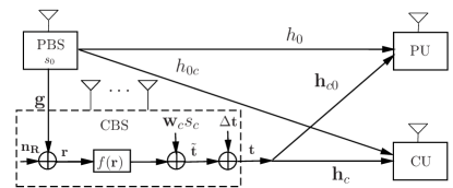
Figure 2: Cooperating Cognitive System Model in the HD mode

II-A System Model

Consider a cooperative cognitive system shown in Fig. 2. The primary system consists of a single-antenna PBS and a single-antenna PU. The cognitive system includes an $N$-antenna ($N>1$) CBS operating in the HD mode and a single-antenna CU . It is assumed that cognitive system is time synchronized with the primary network (this assumption holds for all the investigated schemes). We assume that the quality of the primary link is not good enough to meet its transmission rate target and the cooperation between the CBS and the PBS becomes necessary [1]. To define the system model, we list the following system parameters:

$$h_{0}$$ the scalar channel between the PBS and the PU;

$${h_{0c}}$$ the scalar channel between the PBS and the CU;

$${{\bf h}_{c0}} N\times 1$$ the channel between the CBS and the PU;

$${{\bf h}_{c}} N\times 1$$ the channel between the CBS and the CU;

$${\bf g} N\times 1$$ the channel between the PBS and the CBS;

$$n_{1}$$ the noise received at PU during Phase I

with $$n_{1}\sim\mathcal{CN}(0,1)$$;

$$n_{2}$$ the noise received at PU during Phase II

with $$n_{2}\sim\mathcal{CN}(0,1)$$;

$${\bf n}_{R} N\times 1$$ the noise vector received at the CBS during

Phase I with $${\bf n}_{R}\sim\mathcal{CN}({\bf 0},{\bf I})$$;

$$n_{c}$$ the noise received at the CU during Phase II

with $$n_{c}\sim\mathcal{CN}(0,1)$$;

$$P_{0} \mbox{the available transmit power of the PBS};$$

$$P_{C} \mbox{the available transmit power of the CBS};$$

$$s_{0} s_{0}\sim\mathcal{CN}(0,P_{0})$$ the transmit signal for the PU with ;

$$s_{c} \mbox{the transmit signal for the CU with $s_{c}\sim\mathcal{CN}(0,1)$}.$$

All transmit signal, channel and noise elements are assumed to be independent of each other. We assume global perfect channel state information (CSI) is available at the CBS. In the HD mode, the communication takes place in two phases. In Phase I, the PBS broadcasts its data $s_{0}$, then the received signals at the PU and the CBS are, respectively,

$$y_{1}=h_{0}s_{0}+n_{1},~{}~{}\mbox{and}~{}~{}{\bf r}={\bf g}s_{0}+{\bf n}_{R}.$$ (1)

The CBS processes the received signal and produces $f({\bf r})$ which is defined as

$$f({\bf r})=\left\{\begin{array}[]{ll}{\bf A}{\bf r},&\mbox{for AF where ${\bf A}$ is an $N\times N$ complex}\\ &\mbox{relay matrix;}\\ {\bf w}_{0}\tilde{s}_{0},&\mbox{for DF where ${\bf w}_{0}$ is a beamforming vector}\\ &\mbox{to forward primary signal and $\tilde{s}_{0}=\frac{s_{0}}{\sqrt{P_{0}}}$. }\end{array}\right.$$ (2)

In Phase II, the CBS superimposes the relaying signal $f({\bf r})$ with its own data $s_{c}$ using the cognitive beamforming vector ${\bf w}_{c}$, then transmits to both the PU and the CU. In this phase, the PBS remains idle. The CBS’s transmit signal is

$$\tilde{\bf t}=\left\{\begin{array}[]{ll}{\bf w}_{c}s_{c}+{\bf A}{\bf g}s_{0}+{\bf A}{\bf n}_{R},&\mbox{for AF;}\\ {\bf w}_{c}s_{c}+{\bf w}_{0}\tilde{s}_{0},&\mbox{for DF. }\end{array}\right.$$ (3)

with average power

$$p_{R}={\tt E}\|\tilde{\bf t}\|^{2}=\left\{\begin{array}[]{ll}\|{\bf w}_{c}\|^{2}+P_{0}\|{\bf A}{\bf g}\|^{2}+\|{\bf A}\|^{2},&\mbox{for AF;}\\ \|{\bf w}_{c}\|^{2}+\|{\bf w}_{0}\|^{2},&\mbox{for DF. }\end{array}\right.$$ (4)

To make a fair comparison with the FD mode, we introduce the transmit noise $\Delta{\bf t}$, which combines the effects of phase noise, nonlinear power amplifier, I/Q imbalance, nonlinear low-noise amplifier and ADC impairments [13][26], etc. Then the actually transmitted signal from the CBS is

$${\bf t}=\tilde{\bf t}+\Delta{\bf t},~{}\Delta{\bf t}\sim\mathcal{CN}({\bf 0},P_{t}{\bf I}),\vspace{-2mm}$$ (5)

where $P_{t}$ denotes the transmit noise power and can either be fixed or scale with $p_{R}$, depending on how well these impairments are compensated. It will be seen that in the HD mode, we can use the same approach to solve the problem no matter whether $P_{t}$ is fixed or not. While in the FD mode using the AF protocol, it makes a difference and we will deal with these two cases separately. The received signal at the CU is

$$y_{c}={\bf h}_{c}^{\dagger}{\bf t}+n_{c}$$ (6)

$$=\left\{\begin{array}[]{ll}{\bf h}_{c}^{\dagger}{\bf w}_{c}s_{c}+{\bf h}_{c}^{\dagger}{\bf A}{\bf g}s_{0}+{\bf h}_{c}^{\dagger}{\bf A}{\bf n}_{R}+{\bf h}_{c}^{\dagger}\Delta{\bf t}+n_{c},&\mbox{for AF;}\\ {\bf h}_{c}^{\dagger}{\bf w}_{c}s_{c}+{\bf h}_{c}^{\dagger}{\bf w}_{0}\tilde{s}_{0}+{\bf h}_{c}^{\dagger}\Delta{\bf t}+n_{c},&\mbox{for DF.}\end{array}\right.$$ (9)

The received signal-to-interference plus noise ratio (SINR) at CU is then expressed as

$$\Gamma_{c}=\left\{\begin{array}[]{ll}\frac{|{\bf h}_{c}^{\dagger}{\bf w}_{c}|^{2}}{P_{0}|{\bf h}_{c}^{\dagger}{\bf A}{\bf g}|^{2}+\|{\bf h}_{c}^{\dagger}{\bf A}\|^{2}+P_{t}\|{\bf h}_{c}\|^{2}+1},&\mbox{for AF;}\\ \frac{|{\bf h}_{c}^{\dagger}{\bf w}_{c}|^{2}}{|{\bf h}_{c}^{\dagger}{\bf w}_{0}|^{2}+P_{t}\|{\bf h}_{c}\|^{2}+1},&\mbox{for DF,}\end{array}\right.$$ (10)

and the achievable rate is $R_{c}=\frac{1}{2}\log_{2}(1+\Gamma_{c})$ where the factor $\frac{1}{2}$ arises due to the two orthogonal channel uses. The received signal at the PU is

$$y_{2}={\bf h}_{c0}^{\dagger}{\bf t}+n_{2}$$ (11)

$$=\left\{\begin{array}[]{ll}{\bf h}_{c0}^{\dagger}{\bf w}_{c}s_{c}+{\bf h}_{c0}^{\dagger}{\bf A}{\bf g}s_{0}+{\bf h}_{c0}^{\dagger}{\bf A}{\bf n}_{s}+{\bf h}_{c0}^{\dagger}\Delta{\bf t}+n_{2},&\mbox{for AF;}\\ {\bf h}_{c0}^{\dagger}{\bf w}_{c}s_{c}+{\bf h}_{c0}^{\dagger}{\bf w}_{0}s_{0}+{\bf h}_{c0}^{\dagger}\Delta{\bf t}+n_{2},&\mbox{for DF.}\end{array}\right.$$ (14)

Applying maximum ratio combining (MRC) to $y_{1}$ and $y_{2}$, the received SINR of the PU is the sum of two channel uses, and consequently, the achievable rate is given in (9) at the top of next page.

$$R_{0}=\left\{\begin{array}[]{ll}\frac{1}{2}\log_{2}\left(1+P_{0}|{h}_{0}|^{2}+\frac{P_{0}|{\bf h}_{c0}^{\dagger}{\bf A}{\bf g}|^{2}}{|{\bf h}_{c0}^{\dagger}{\bf w}_{c}|^{2}+\|{\bf h}_{c0}^{\dagger}{\bf A}\|^{2}+P_{t}\|{\bf h}_{c0}\|^{2}+1}\right),\mbox{for AF;}&\\ \frac{1}{2}\log_{2}\left(1+P_{0}|h_{0}|^{2}+\min\left(P_{0}\|{\bf g}\|^{2},\frac{|{\bf h}_{c0}^{\dagger}{\bf w}_{0}|^{2}}{|{\bf h}_{c0}^{\dagger}{\bf w}_{c}|^{2}+P_{t}\|{\bf h}_{c0}\|^{2}+1}\right)\right),\mbox{for DF.}&\end{array}\right.$$ (15)

 

II-B Achievable Rate Region and Problem Formulation

The problem of interest is to find the rate region given the primary and cognitive power constraints. To achieve this, we propose to maximize the CU rate $R_{c}$ subject to the PU’s rate constraint $r_{0}$ and the CBS’s transmit power constraint $P_{C}$, by jointly optimizing the cognitive beamforming vector ${\bf w}_{c}$, the relaying processing matrix ${\bf A}$ and the forwarding beamforming vector ${\bf w}_{0}$ for both AF and DF. Mathematically, the optimization problem can be written as

$$\max~{}R_{c}~{}~{}~{}~{}\mbox{s.t.}~{}~{}~{}R_{0}\geq r_{0},~{}~{}p_{R}\leq P_{C},$$ (16)

where the optimization variables are $({\bf w}_{c},{\bf A})$, $({\bf w}_{c},{\bf w}_{0})$ for AF and DF, respectively. Using the monotonicity between the received SINR and the achievable rate, we can derive simplified equivalent problem formulations for AF and DF. More specifically, we have (11) at the top of next page

$$\mbox{P-AF-HD:}~{}~{}\max_{{\bf w}_{c},{\bf A}} \frac{|{\bf h}_{c}^{\dagger}{\bf w}_{c}|^{2}}{P_{0}|{\bf h}_{c}^{\dagger}{\bf A}{\bf g}|^{2}+\|{\bf h}_{c}^{\dagger}{\bf A}\|^{2}+P_{t}\|{\bf h}_{c}\|^{2}+1}$$ (17)

s.t. $$\frac{|{\bf h}_{c0}^{\dagger}{\bf A}{\bf g}|^{2}}{|{\bf h}_{c0}^{\dagger}{\bf w}_{c}|^{2}+\|{\bf h}_{c0}^{\dagger}{\bf A}\|^{2}+P_{t}\|{\bf h}_{c0}\|^{2}+1}\geq\gamma_{0_{AF}}^{{}^{\prime}},$$

$$\|{\bf w}_{c}\|^{2}+P_{0}\|{\bf A}{\bf g}\|^{2}+\|{\bf A}\|^{2}\leq P_{C},$$

 

and

$$\mbox{P-DF-HD:}~{}~{}\max_{{\bf w}_{0},{\bf w}_{c}} \frac{|{\bf h}_{c}^{\dagger}{\bf w}_{c}|^{2}}{|{\bf h}_{c}^{\dagger}{\bf w}_{0}|^{2}+P_{t}\|{\bf h}_{c}\|^{2}+1}$$ (18)

s.t. $$P_{0}\|{\bf g}\|^{2}\geq\gamma_{0_{DF}}^{{}^{\prime}},$$

$$\frac{|{\bf h}_{c0}^{\dagger}{\bf w}_{0}|^{2}}{|{\bf h}_{c0}^{\dagger}{\bf w}_{c}|^{2}+P_{t}\|{\bf h}_{c0}\|^{2}+1}\geq\gamma_{0_{DF}}^{{}^{\prime}},$$

$$\|{\bf w}_{c}\|^{2}+\|{\bf w}_{0}\|^{2}\leq P_{C},$$

where $\gamma_{0_{AF}}^{{}^{\prime}}\triangleq\frac{2^{2r_{0}}-1}{P_{0}}-|h_{0}|^{2}$ and $\gamma_{0_{DF}}^{{}^{\prime}}\triangleq 2^{2r_{0}}-1-P_{0}|{h}_{0}|^{2}$. Obviously, P-AF-HD appears more complicated than P-DF-HD, so we first focus on P-AF-HD and we later show that actually both problems can be solved using the same mechanism.

II-C The Optimal Structure of ${\bf A}$ in P-AF-HD and Physical Interpretation

Problem P-AF-HD involves the optimization of an $N\times N$ matrix ${\bf A}$. In the following theorem we will characterize the optimal structure of ${\bf A}$.

Theorem 1

The optimal AF relay matrix ${\bf A}$ has the structure of

$${\bf A}={\bf w}_{a}{\bf g}^{\dagger},$$ (19)

where $\bar{\bf H}\triangleq[{\bf h}_{c0}~{}{\bf h}_{c}]$, ${\bf w}_{a}=\bar{\bf H}{\bf b}$ and ${\bf b}\in\mathbb{C}^{2\times 1}$ are parameter vectors.

The proof is given in Appendix A. The structure of ${\bf A}={\bf w}_{a}{\bf g}^{\dagger}$ reveals its two functions. First it coherently amplifies the received primary signals at different receive antennas using MRC receiver ${\bf g}^{\dagger}$ to produce a noisy version of the primary signal; then fowards the noisy primary signal using the transmit beamforming vector ${\bf w}_{a}$. Theorem 1 not only provides physical interpretation about the above mentioned relay processing but also greatly simplifies problem P-AF-HD, which will be seen in the next subsection.

II-D Simplified AF Problem

It is noted that ${\bf A}$ originally is a general $N\times N$ matrix while (19) indicates that it is actually a rank-1 matrix and can be represented by a new vector ${\bf w}_{a}$. Employing this structure, the problem P-AF-HD in (17) is simplified to

$$\min_{{\bf w}_{c},{\bf w}_{a}} \frac{|{\bf h}_{c}^{\dagger}{\bf w}_{c}|^{2}}{(P_{0}\|{\bf g}\|^{4}+\|{\bf g}\|^{2})|{\bf h}_{c}^{\dagger}{\bf w}_{a}|^{2}+P_{t}\|{\bf h}_{c}\|^{2}+1}$$ (20)

s.t. $$\frac{|{\bf h}_{c0}^{\dagger}{\bf w}_{a}|^{2}}{|{\bf h}_{c0}^{\dagger}{\bf w}_{c}|^{2}+P_{t}\|{\bf h}_{c0}\|^{2}+1}\geq\frac{\gamma_{0_{AF}}^{{}^{\prime}}}{(\|{\bf g}\|^{4}-\gamma_{0_{AF}}^{{}^{\prime}}\|{\bf g}\|^{2})},$$

$$\|{\bf w}_{c}\|^{2}+(P_{0}\|{\bf g}\|^{4}+\|{\bf g}\|^{2})\|{\bf w}_{a}\|^{2}\leq P_{C}.$$

For the sake of presentation, the closed-form solution to the above problem in a general form is given in Appendix B. From the right hand side of the first constraint, it is observed that the problem is feasible or the required PU rate can be satisfied only when $\|{\bf g}\|^{2}>\gamma_{0_{AF}}^{{}^{\prime}}$, which complies with the common sense that the end-to-end performance of an AF relay system is upper bounded by the channel quality of the PBS-CBS link ${\bf g}$; if this link is too weak, the CBS can not assist the primary transmission.

For solving problem P-DF-HD in (18), we can first check whether the first constraint is satisfied; if yes, we can remove this constraint and the remaining of the problem has the same structure as (20), then its solution is given in Appendix B; otherwise, the problem is deemed infeasible meaning that the required primary rate cannot be supported even with the assistance from the CBS.

III FD-CBS System Model and Optimization

III-A System Model

In this section, we consider that the CBS operates in the FD mode, i.e., the CBS can receive and transmit data at the same time and frequency. We assume the CBS has $N_{r}$ receive antennas/RF chains and $N_{t}$ transmit antennas/RF chains. Due to the FD mode, the receive antennas of the CBS will receive a self-interference from its transmit antennas. The system parameters that are different from the HD based system model are defined as follows:

$${{\bf h}_{c0_{FD}}} N_{t}\times 1$$ the channel between the CBS and the PU;

$${{\bf h}_{c_{FD}}} N_{t}\times 1$$ the channel between the CBS and the CU;

$${\bf g}_{FD} N_{r}\times 1$$ the channel between the PBS and the CBS;

$${\bf n}_{R_{FD}} N_{r}\times 1$$ the noise vector received at the CBS

with $${\bf n}_{R_{FD}}\sim\mathcal{CN}({\bf 0},{\bf I})$$;

$$n_{0} n_{0}\sim\mathcal{CN}(0,1)$$ the noise received at the PU with ;

$${\bf H} N_{r}\times N_{t}$$ the equivalent loop interference channel

matrix at the CBS;

$$P_{C_{FD}}$$ the transmit power constraint of the CBS;

$$P_{0_{FD}} \mbox{the transmit power of the PBS}.$$

We may reuse some variables from the HD mode when no confusion occurs. It is worth noting that ${\bf H}$ is the equivalent loop interference channel after the self-interference mitigation [10][11], and its strength depends on the quality of the mitigation process that can be performed with techniques such as antenna separation and analog-domain self-interference cancellation, etc.

Although FD and HD are characterized by fundamental operational and complexity differences, the purpose of our study is to provide a fair comparison between the two relaying modes. This fair comparison is supported by the following assumptions:

• We ensure the same energy consumptions for both modes that is expressed as $P_{C_{FD}}=\frac{P_{C}}{2}$ and $P_{0_{FD}}=\frac{P_{0}}{2}$ [15].

• We assume the same number of total antennas i.e., an FD system has $N_{t}$ transmit and $N_{r}$ receive antennas and an HD system with a total of $N=N_{r}+N_{t}$ antennas. More specificaly:

  • In the HD mode, the CBS has $N_{r}$ receive RF chains and $N_{t}$ transmit RF chains and it uses equal number of antennas: $N_{r}$ receive antennas in Phase I and $N_{t}$ transmit antennas in Phase II. In this setting, both the FD and HD systems have the same antenna configuration.

  • In addition, we also consider a case that the HD mode has higher cost: in the HD mode, the CBS has $N$ transmit RF chains and $N$ receive RF chains, so it can use all $N$ receive antennas in Phase I and all $N$ transmit antennas in Phase II.

Obviously the performance of 2) is superior to that of 1) but with the cost of extra complexity. We will evaluate the performance of both cases in Section V.

The details of FD relay processing are illustrated in Fig. 3.

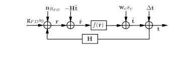
Figure 3: Relay processing at the FD CBS

We use the index $i$ to denote time instant. The received signal at the PBS and the CBS are, respectively,

$$y[i] = h_{0}s_{0}[i]+{\bf h}_{c0_{FD}}^{\dagger}(\tilde{\bf t}[i]+\Delta{\bf t}[i])+n_{0}[i],$$ (21)

$${\bf r}[i] = {\bf g}s_{0}[i]+{\bf H}(\tilde{\bf t}[i]+\Delta{\bf t}[i])+{\bf n}_{R_{FD}}[i],$$ (22)

where $\tilde{\bf t}[i]+\Delta{\bf t}[i]$ is the actual transmitted signal from the CBS. The transmit Gaussian noise vector is denoted as $\Delta{\bf t}$ as the HD mode, $P_{t}$ denotes the noise power and $\tilde{\bf t}[i]$ is the known transmit signal from the CBS including both relaying primary signal and cognitive signal:

$$\tilde{\bf t}[i]=f(\hat{\bf r}(i-D))+{\bf w}_{c}s_{c}[i],$$ (23)

where $\hat{\bf r}$ is the pre-processed received signal at the CBS and $D>0$ is the processing delay. This delay $D>0$ is a general assumption and refers to the required processing time in order to implement the FD operation [15]. In practical systems the processing delay for the AF scheme is much smaller than the one in the DF case; however our analysis is general and holds for any $D>0$.

The relay processing at the CBS is defined as:

$$f(\hat{\bf r})=\left\{\begin{array}[]{cl}{\bf A}\hat{\bf r},&\mbox{for AF where ${\bf A}$ is an $N_{t}\times N_{r}$ relay matrix;}\\ {\bf w}_{0}\tilde{s}_{0},&\mbox{for DF where ${\bf w}_{0}$ is a beamforming vector,}\\ &\mbox{$\tilde{s}_{0}=\frac{s_{0}}{\sqrt{P_{0_{F}D}}}$. }\end{array}\right.$$ (24)

Although the channel ${\bf H}$ is perfectly estimated at the CBS and the CBS can perfectly remove the noise component ${\bf H}\tilde{\bf t}[i]$, but the term ${\bf H}\tilde{\Delta}{\bf t}[i]$ remains and forms the residual interference that affects the CBS’s input. As a result the CBS gets pre-processed signal

$$\hat{\bf r}[i]={\bf r}[i]-{\bf H}\tilde{\bf t}[i]={\bf g}s_{0}[i]+{\bf H}\Delta{\bf t}[i]+{\bf n}_{R_{FD}}[i].$$ (25)

Suppose the CBS further processes $\hat{\bf r}[i]$, then

$$\tilde{\bf t}[i]=\left\{\begin{array}[]{ll}{\bf A}\hat{\bf r}[i-D]+{\bf w}_{c}s_{c}[i]={\bf A}{\bf g}s_{0}[i-D]+\\ {\bf A}{\bf H}\Delta{\bf t}[i-D]+{\bf A}{\bf n}_{r}[i-D]+{\bf w}_{c}s_{c}[i],&\\ \mbox{for AF where ${\bf A}$ is an $N\times N_{r}$ matrix};&\\ {\bf w}_{0}\tilde{s}_{0}[i-D]+{\bf w}_{c}s_{c}[i],&\\ \mbox{for DF where~{}}\tilde{s}_{0}[i-D]=\frac{s_{0}[i-D]}{|s_{0}[i-D]|}&\end{array}\right.$$ (26)

with average power

$$p_{R_{FD}}={\tt E}(\|\tilde{\bf t}\|^{2})=\left\{\begin{array}[]{ll}P_{0_{FD}}\|{\bf A}{\bf g}_{FD}\|^{2}+P_{t}\|{\bf A}{\bf H}\|^{2}+\|{\bf A}\|^{2}\\ +\|{\bf w}_{c}\|^{2},\mbox{for AF;}&\\ \|{\bf w}_{0}\|^{2}+\|{\bf w}_{c}\|^{2},\mbox{for DF.}&\end{array}\right.$$ (27)

The received signal at the CU is

$$y_{c}[i]={\bf h}_{c_{FD}}^{\dagger}(\tilde{\bf t}[i]+\Delta{\bf t}[i])+{h}_{0c}s_{0}[i]+n_{c}[i]$$

$$=\left\{\begin{array}[]{ll}{\bf h}_{c_{FD}}^{\dagger}{\bf w}_{c}s_{c}[i]+{\bf h}_{c_{FD}}^{\dagger}{\bf A}{\bf g}s_{0}[i-D]+{\bf h}_{c_{FD}}^{\dagger}{\bf A}{\bf H}\Delta{\bf t}\\ +{\bf h}_{c_{FD}}^{\dagger}{\bf A}{\bf n}_{R_{FD}}[i-D]+{\bf h}_{c_{FD}}^{\dagger}\Delta{\bf t}[i]+h_{0c}s_{0}[i]+n_{c}[i],&\\ \mbox{for AF;}&\\ {\bf h}_{c_{FD}}^{\dagger}{\bf w}_{c}s_{c}[i]+{\bf h}_{c_{FD}}^{\dagger}{\bf w}_{0}s_{0}[i-D]+{\bf h}_{c_{FD}}^{\dagger}\Delta{\bf t}[i]\\ +h_{0c}s_{0}[i]+n_{c}[i],&\\ \mbox{for DF.}&\end{array}\right.$$ (32)

The received SINR $\Gamma_{c_{FD}}$ at CU is expressed in (33).

$$\Gamma_{c_{FD}}=\left\{\begin{array}[]{ll}\frac{|{\bf h}_{c_{FD}}^{\dagger}{\bf w}_{c}|^{2}}{P_{0_{FD}}|{\bf h}_{c_{FD}}^{\dagger}{\bf A}{\bf g}|^{2}+P_{t}\|{\bf h}_{c_{FD}}^{\dagger}{\bf A}{\bf H}\|^{2}+P_{t}\|{\bf h}_{c_{FD}}\|^{2}+\|{\bf h}_{c_{FD}}^{\dagger}{\bf A}\|^{2}+P_{0_{FD}}|{h}_{0c}|^{2}+1},&\mbox{for AF;}\\ \frac{|{\bf h}_{c_{FD}}^{\dagger}{\bf w}_{c}|^{2}}{|{\bf h}_{c_{FD}}^{\dagger}{\bf w}_{0}|^{2}+P_{t}\|{\bf h}_{c_{FD}}\|^{2}+P_{0_{FD}}|h_{0c}|^{2}+1},&\mbox{for DF.}\end{array}\right.$$ (33)

Then the achievable CU rate is $R_{c_{FD}}=\log_{2}(1+\Gamma_{c_{FD}})$. It is worth nothing that due to the FD, the CU rate does not suffer from the loss of a prelog factor $\frac{1}{2}$ observed in the HD mode. However, due to the residual self-interference, for AF, there is an additional interference term $P_{t}\|{\bf h}_{c_{FD}}^{\dagger}{\bf A}{\bf H}\|^{2}$ compared to the HD mode.

The received signal at the PU is shown in (37).

$$y[i] = h_{0}s_{0}[i]+{\bf h}_{c0_{FD}}^{\dagger}(\tilde{\bf t}[i]\Delta{\bf t}[i])+n_{0}[i]$$ (37)

$$= \left\{\begin{array}[]{ll}h_{0}s_{0}[i]+{\bf h}_{c0_{FD}}^{\dagger}{\bf A}{\bf g}s_{0}[i-D]+{\bf h}_{c0_{FD}}^{\dagger}{\bf A}{\bf H}\Delta{\bf t}[i]\\ ~{}~{}~{}~{}~{}~{}~{}+{\bf h}_{c0_{FD}}^{\dagger}{\bf A}{\bf n}_{r}[i-D]+{\bf h}_{c0_{FD}}^{\dagger}{\bf w}_{c}s_{c}[i]+{\bf h}_{c0_{FD}}^{\dagger}\Delta{\bf t}+n_{0}[i],&\mbox{for AF;}\\ h_{0}s_{0}[i]+{\bf h}_{c0_{FD}}^{\dagger}{\bf w}_{0}s_{0}[i-D]+{\bf h}_{c0_{FD}}^{\dagger}{\bf w}_{c}s_{c}[i]+{\bf h}_{c0_{FD}}^{\dagger}\Delta{\bf t}[i]+n_{0}[i],&\mbox{for DF.}\end{array}\right.$$

Since the direct link channel $h_{0}$ is weak, the PU simply treats $h_{0}s_{0}[i]$ as noise and decodes $s_{0}[i-D]$, therefore, the received SINR at the PU is given in (38)

$$\Gamma_{0_{FD}}=\left\{\begin{array}[]{ll}\frac{P_{0_{FD}}|{\bf h}_{c0_{FD}}^{\dagger}{\bf A}{\bf g}|^{2}}{P_{0_{FD}}|h_{0}|^{2}+P_{t}\|{\bf h}_{c0_{FD}}^{\dagger}{\bf A}{\bf H}\|^{2}+P_{t}\|{\bf h}_{c0_{FD}}\|^{2}+\|{\bf h}_{c0_{FD}}^{\dagger}{\bf A}\|^{2}+|{\bf h}_{c0_{FD}}^{\dagger}{\bf w}_{c}|^{2}+1},&\mbox{for AF;}\\ \frac{P_{0_{FD}}|{\bf h}_{c0_{FD}}^{\dagger}{\bf w}_{0}|^{2}}{P_{0_{FD}}|{h}_{0}|^{2}+P_{t}\|{\bf h}_{c0_{FD}}\|^{2}+|{\bf h}_{c0_{FD}}^{\dagger}{\bf w}_{c}|^{2}+1},&\mbox{for DF.}\end{array}\right.$$ (38)

The achievable rate for the PU is provide in (39).

$$R_{0_{FD}}=\left\{\begin{array}[]{ll}\log_{2}\left(1+\frac{P_{0_{FD}}|{\bf h}_{c0_{FD}}^{\dagger}{\bf A}{\bf g}|^{2}}{P_{0_{FD}}|h_{0}|^{2}+P_{t}\|{\bf h}_{c0_{FD}}^{\dagger}{\bf A}{\bf H}\|^{2}+P_{t}\|{\bf h}_{c0_{FD}}\|^{2}+\|{\bf h}_{c0_{FD}}^{\dagger}{\bf A}\|^{2}+|{\bf h}_{c0_{FD}}^{\dagger}{\bf w}_{c}|^{2}+1}\right),&\mbox{for AF;}\\ \log_{2}\left(1+\min\left(P_{0_{FD}}\|{\bf g}_{FD}\|^{2},\frac{P_{0_{FD}}|{\bf h}_{c0_{FD}}^{\dagger}{\bf w}_{0}|^{2}}{P_{0_{FD}}|{h}_{0}|^{2}+P_{t}\|{\bf h}_{c0_{FD}}\|^{2}+|{\bf h}_{c0_{FD}}^{\dagger}{\bf w}_{c}|^{2}+1}\right)\right),&\mbox{for DF.}\end{array}\right.$$ (39)

III-B Problem Formulation

Similar to the HD case, we will study the achievable rate region by solving the CU SINR maximization problems subject to the PU rate constraint $r_{0}$ and the CBS power constraint $P_{C_{FD}}$. The problems for AF and DF are formulated as (III-B)

P-FD-AF:

$$~{}\max_{{\bf A},{\bf w}_{c}} \frac{|{\bf h}_{c_{FD}}^{\dagger}{\bf w}_{c}|^{2}}{P_{0_{FD}}|{\bf h}_{c_{FD}}^{\dagger}{\bf A}{\bf g}_{FD}|^{2}+P_{t}\|{\bf h}_{c_{FD}}^{\dagger}{\bf A}{\bf H}\|^{2}+P_{t}\|{\bf h}_{c_{FD}}\|^{2}+\|{\bf h}_{c_{FD}}^{\dagger}{\bf A}\|^{2}+P_{0_{FD}}|{h}_{0c}|^{2}+1}$$ (40)

s.t. $$\frac{P_{0_{FD}}|{\bf h}_{c0_{FD}}^{\dagger}{\bf A}{\bf g}|^{2}}{P_{0_{FD}}|h_{0}|^{2}+P_{t}\|{\bf h}_{c0_{FD}}^{\dagger}{\bf A}{\bf H}\|^{2}+P_{t}\|{\bf h}_{c0_{FD}}\|^{2}+\|{\bf h}_{c0_{FD}}^{\dagger}{\bf A}\|^{2}+|{\bf h}_{c0_{FD}}^{\dagger}{\bf w}_{c}|^{2}+1}$$

$$\geq\gamma_{0_{FD}}\triangleq 2^{\gamma_{0}}-1,$$

$$p_{R_{FD}}=P_{0_{FD}}\|{\bf A}{\bf g}_{FD}\|^{2}+P_{t}\|{\bf A}{\bf H}\|^{2}+\|{\bf A}\|^{2}+\|{\bf w}_{c}\|^{2}\leq P_{C_{FD}},$$

and (27) on next page.

P-FD-DF:

$$~{}\max_{{\bf w}_{0},{\bf w}_{c}} \frac{|{\bf h}_{c_{FD}}^{\dagger}{\bf w}_{c}|^{2}}{|{\bf h}_{c_{FD}}^{\dagger}{\bf w}_{0}|^{2}+P_{t}\|{\bf h}_{c_{FD}}\|^{2}+P_{0_{FD}}|{h}_{0c}|^{2}+1}$$ (41)

s.t. $$\frac{P_{0_{FD}}\|{\bf g}_{FD}\|^{2}}{P_{t}\|{\bf H}\|^{2}+1}\geq\gamma_{0_{FD}}$$

$$\frac{|{\bf h}_{c0_{FD}}^{\dagger}{\bf w}_{0}|^{2}}{|{\bf h}_{c0_{FD}}^{\dagger}{\bf w}_{c}|^{2}+P_{t}\|{\bf h}_{c0_{FD}}\|^{2}+P_{0_{FD}}|{h}_{0}|^{2}+1}\geq\gamma_{0_{FD}}$$

$$p_{R_{FD}}=\|{\bf w}_{0}\|^{2}+\|{\bf w}_{c}\|^{2}\leq P_{C_{FD}}.$$

Comparing to P-HD-AF, it can be checked that the optimal relay processing matrix ${\bf A}$ in P-FD-AF possesses the same structure ${\bf A}={\bf w}_{a}{\bf g}_{FD}^{\dagger}$ as HD in Theorem 1 and as a result, the problem P-FD-AF is reformulated as (42).

$$\max_{{\bf w}_{a},{\bf w}_{c}} \frac{|{\bf h}_{c_{FD}}^{\dagger}{\bf w}_{c}|^{2}}{(1+P_{0_{FD}}|h_{0c}|^{2}+P_{t}\|{\bf h}_{c_{FD}}\|^{2})+(P_{0_{FD}}\|{\bf g}_{FD}\|^{4}+P_{t}\|{\bf g}_{FD}^{\dagger}{\bf H}\|^{2}+\|{\bf g}_{FD}\|^{2})|{\bf h}_{c_{FD}}^{\dagger}{\bf w}_{a}\|^{2}}$$ (42)

s.t. $$\frac{|{\bf h}_{c0_{FD}}^{\dagger}{\bf w}_{a}|^{2}}{(1+P_{t}\|{\bf h}_{c0_{FD}}\|^{2}+P_{0_{FD}}|h_{0}|^{2})+|{\bf h}_{c0_{FD}}^{\dagger}{\bf w}_{c}|^{2}}\geq\frac{\gamma_{0_{FD}}}{(P_{0_{FD}}\|{\bf g}_{FD}\|^{4}-\gamma_{0_{FD}}(\|{\bf g}_{FD}\|^{2}+P_{t}\|{\bf g}_{FD}^{\dagger}{\bf H}\|^{2}))}$$

$$(P_{0_{FD}}\|{\bf g}_{FD}\|^{4}+\|{\bf g}_{FD}\|^{2}+P_{t}\|{\bf g}_{FD}^{\dagger}{\bf H}\|^{2})\|{\bf w}_{a}\|^{2}+\|{\bf w}_{c}\|^{2}\leq P_{C_{FD}}.$$

III-C Fixed Transmit Noise $P_{t}$

In our previous discussions, we have assumed that $P_{t}$ is fixed which corresponds to an efficient interference cancellation process. With this assumption, (42) has the same structure as (20) for AF, and (III-B) and (18) share the same structure for DF, therefore all solutions can be found using the approach presented in Appendix B.

III-D Scalable Transmit Noise $P_{t}$

Although fixing the transmit noise power $P_{t}$ simplifies the problem and the solution, in practice, it is more feasible to assume that $P_{t}$ scales with the CBS transmit power, i.e., $P_{t}=\epsilon^{2}p_{R}$ and $P_{t}=\epsilon^{2}p_{R_{FD}}$ for the HD and FD modes, respectively, where $\epsilon^{2}$ is a scaling factor and denotes the percentage of the transmit noise power to the total CBS transmit power. It depends on the hardware impairments and can be assumed that it is small for efficient implementations. In this case, the CBS may not use its full power since more power brings more noise to the receivers in both modes and more self-interference in the FD mode.

Notice that in the HD mode, we have not discussed this issue for the problem formulations P-DF-HD in (18) and P-AF-HD in (20), respectively, and the reason is as follows. When $P_{t}$ scales with $p_{R}$, the objective functions in both (18) and (20) are non-decreasing functions of $p_{R}$, which means the relay should always use the maximum transmit power $p_{R}=P_{C}$. We illustrate this by taking the problem P-AF-HD for example. With $P_{t}=\epsilon^{2}p_{R}$, it becomes

$$\max_{{\bf w}_{c},{\bf A},p_{R}} \frac{|{\bf h}_{c}^{\dagger}{\bf w}_{c}|^{2}}{P_{0}|{\bf h}_{c}^{\dagger}{\bf A}{\bf g}|^{2}+\|{\bf h}_{c}^{\dagger}{\bf A}\|^{2}+\epsilon^{2}p_{R}\|{\bf h}_{c}\|^{2}+1}$$ (43)

s.t. $$\frac{|{\bf h}_{c0}^{\dagger}{\bf A}{\bf g}|^{2}}{|{\bf h}_{c0}^{\dagger}{\bf w}_{c}|^{2}+\|{\bf h}_{c0}^{\dagger}{\bf A}\|^{2}+\epsilon^{2}p_{R}\|{\bf h}_{c0}\|^{2}+1}\geq\gamma_{0_{AF}}^{{}^{\prime}},$$

$$p_{R}=\|{\bf w}_{c}\|^{2}+P_{0}\|{\bf A}{\bf g}\|^{2}+\|{\bf A}\|^{2}\leq P_{C}.$$

Suppose its optimal solution is $({\bf w}_{c}^{*},{\bf A}^{*},p_{R}^{*})$ and the corresponding optimal objective value is $\gamma_{c}^{*}$. We assume the CBS does not use maximum transmit power, i.e., $p_{R}^{*}=\frac{1}{\alpha}P_{C},\alpha>1$. Then we construct another solution $(\sqrt{\alpha}{\bf w}_{c}^{*},\sqrt{\alpha}{\bf A}^{*},\alpha p_{R}^{*})$, which satisfies both constraints and gives higher objective value $\frac{|{\bf h}_{c}^{\dagger}{\bf w}_{c}^{*}|^{2}}{P_{0}|{\bf h}_{c}^{\dagger}{\bf A}^{*}{\bf g}|^{2}+\|{\bf h}_{c}^{\dagger}{\bf A}^{*}\|^{2}+\epsilon^{2}p_{R}^{*}\|{\bf h}_{c}\|^{2}+\frac{1}{\alpha}}>\gamma_{c}^{*}$. This contradicts the fact that $({\bf w}_{c}^{*},{\bf A}^{*},p_{R}^{*})$ is the optimal solution, therefore it must hold that $p_{R}=P_{C}$.

For the FD mode, we next show that the scalable noise does not affect the approach to solve the problem P-FD-DF in (III-B). With substitution $P_{t}=\epsilon^{2}p_{R_{FD}}$, it is easy to see that the first constraint is equivalent to

$$p_{R_{FD}}\leq\frac{\frac{P_{0_{FD}}\|{\bf g}_{FD}\|^{2}}{\gamma_{0_{FD}}}-1}{\epsilon^{2}\|{\bf H}\|^{2}}.$$ (44)

Then P-FD-DF becomes (31).

$$\max_{{\bf w}_{0},{\bf w}_{c},p_{R_{FD}}}~{}\frac{|{\bf h}_{c_{FD}}^{\dagger}{\bf w}_{c}|^{2}}{|{\bf h}_{c_{FD}}^{\dagger}{\bf w}_{0}|^{2}+\epsilon^{2}p_{R_{FD}}\|{\bf h}_{c_{FD}}\|^{2}+P_{0_{FD}}|{h}_{0c}|^{2}+1}$$ (45)

$$\mbox{s.t.}~{}\frac{|{\bf h}_{c0_{FD}}^{\dagger}{\bf w}_{0}|^{2}}{|{\bf h}_{c0_{FD}}^{\dagger}{\bf w}_{c}|^{2}+\epsilon^{2}p_{R_{FD}}\|{\bf h}_{c0_{FD}}\|^{2}+P_{0_{FD}}|{h}_{0}|^{2}+1}\geq\gamma_{0_{FD}},$$

$$p_{R_{FD}}=\|{\bf w}_{0}\|^{2}+\|{\bf w}_{c}\|^{2}\leq\bar{P}_{C_{FD}}$$

$$\triangleq\min\left(P_{C_{FD}},\max\left(0,\frac{\frac{P_{0_{FD}}\|{\bf g}_{FD}\|^{2}}{\gamma_{0_{FD}}}-1}{\epsilon^{2}\|{\bf H}\|^{2}}\right)\right).$$

Problem (45) has the similar structure as (43) and at the optimum, it must hold that $p_{R_{FD}}=\bar{P}_{C_{FD}}$. To summarize, the scalable transmit noise power does not affect the mechanism to solve the problems for the HD mode and the FD mode with DF relaying protocol.

However, the above remark may not be true for the FD mode when AF protocol is used since the CBS amplifies the received noise and more transmit power results in more self-interference. We will study this problem in the remaining of this section.

With substitution $P_{t}=\epsilon^{2}p_{R_{FD}}$, problem (42) is updated to (III-D).

$$\mathbb{P}1: \max_{{\bf w}_{a},{\bf w}_{c},p_{R_{FD}}}\frac{|{\bf h}_{c_{FD}}^{\dagger}{\bf w}_{c}|^{2}}{(1+P_{0_{FD}}|h_{0c}|^{2}+\epsilon^{2}p_{R}\|{\bf h}_{c_{FD}}\|^{2})+(P_{0_{FD}}\|{\bf g}_{FD}\|^{4}+\epsilon^{2}p_{R_{FD}}\|{\bf g}_{FD}^{\dagger}{\bf H}\|^{2}+\|{\bf g}_{FD}\|^{2})|{\bf h}_{c_{FD}}^{\dagger}{\bf w}_{a}\|^{2}}$$

s.t. $$\frac{|{\bf h}_{c0_{FD}}^{\dagger}{\bf w}_{a}|^{2}}{(1+\epsilon^{2}p_{R_{FD}}\|{\bf h}_{c0_{FD}}\|^{2}+P_{0_{FD}}|h_{0}|^{2})+|{\bf h}_{c0_{FD}}^{\dagger}{\bf w}_{c}|^{2}}\geq\frac{\gamma_{0_{FD}}}{(P_{0_{FD}}\|{\bf g}_{FD}\|^{4}-\gamma_{0_{FD}}(\|{\bf g}_{FD}\|^{2}+\epsilon^{2}p_{R_{FD}}\|{\bf g}_{FD}^{\dagger}{\bf H}\|^{2}))},$$ (46)

$$p_{R_{FD}}=(P_{0_{FD}}\|{\bf g}_{FD}\|^{4}+\|{\bf g}_{FD}\|^{2}+\epsilon^{2}p_{R_{FD}}\|{\bf g}_{FD}^{\dagger}{\bf H}\|^{2})\|{\bf w}_{a}\|^{2}+\|{\bf w}_{c}\|^{2}\leq P_{C_{FD}}.$$

Problem $\mathbb{P}1$ is quite complicated since the CBS power constraint is not always active and it involves the product of two quadratic terms. We denote its objective value as a function of available CBS power $P_{C_{FD}}$, i.e., $\Psi(P_{C_{FD}})$. To solve it, we first focus on the following problem $\mathbb{P}2$ whose objective is $\Phi(P)$, a function of a parameter $P$ in (III-D).

$$\mathbb{P}2: \Phi(P)=\max_{{\bf w}_{a},{\bf w}_{c}}\frac{|{\bf h}_{c_{FD}}^{\dagger}{\bf w}_{c}|^{2}}{(1+P_{0_{FD}}|h_{0c}|^{2}+\epsilon^{2}P\|{\bf h}_{c_{FD}}\|^{2})+(P_{0_{FD}}\|{\bf g}_{FD}\|^{4}+\epsilon^{2}P\|{\bf g}_{FD}^{\dagger}{\bf H}\|^{2}+\|{\bf g}_{FD}\|^{2})|{\bf h}_{c_{FD}}^{\dagger}{\bf w}_{a}\|^{2}}$$

s.t. $$\frac{|{\bf h}_{c0_{FD}}^{\dagger}{\bf w}_{a}|^{2}}{(1+\epsilon^{2}P\|{\bf h}_{c0_{FD}}\|^{2}+P_{0_{FD}}|h_{0}|^{2})+|{\bf h}_{c0_{FD}}^{\dagger}{\bf w}_{c}|^{2}}\geq\frac{\gamma_{0_{FD}}}{(P_{0_{FD}}\|{\bf g}_{FD}\|^{4}-\gamma_{0_{FD}}(\|{\bf g}_{FD}\|^{2}+\epsilon^{2}P\|{\bf g}_{FD}^{\dagger}{\bf H}\|^{2}))},$$ (47)

$$(P_{0_{FD}}\|{\bf g}_{FD}\|^{4}+\|{\bf g}_{FD}\|^{2}+\epsilon^{2}P\|{\bf g}_{FD}^{\dagger}{\bf H}\|^{2})\|{\bf w}_{a}\|^{2}+\|{\bf w}_{c}\|^{2}\leq P.$$

The following theorem characterizes the relation between $\mathbb{P}1$ and $\mathbb{P}2$.

Theorem 2

Assuming that $\mathbb{P}1$ is feasible, it can be solved by considering $\mathbb{P}2$, i.e., $\Psi(P_{C_{FD}})=\max_{0\leq P\leq P_{C_{FD}}}\Phi(P)$.

Proof:

The proof is based on the following two observations.

• Suppose the optimal solution to $\mathbb{P}1$ is given by $({\bf w}_{0}^{*},{\bf w}_{c}^{*},p_{R}^{*})$ and it is easy to see that $\Psi(P_{C_{FD}})=\Phi(p_{R}^{*})\leq\max_{0\leq P\leq P_{C_{FD}}}\Phi(P)$.

• On the other hand, given an input power $P\leq P_{C_{FD}}$, we can solve $\mathbb{P}2$ to obtain $({\bf w}_{0}^{p},{\bf w}_{c}^{p})$ and suppose its objective is $\Phi(P)$. Following the same argument for (43), we can see that with the optimal solution, the last constraint of $\mathbb{P}2$ must be satisfied with equality. Therefore $({\bf w}_{0}^{p},{\bf w}_{c}^{p},P)$ is also a feasible solution to $\mathbb{P}1$, and this implies that $\Phi(P)\leq\Psi(P_{C_{FD}}),\forall~{}0\leq P\leq P_{C}$.

Combining the above two facts, we conclude that $\Psi(P_{C_{FD}})$ equals the maximum of $\Phi(P),0\leq P\leq P_{C_{FD}}$. ∎

Theorem 2 indicates that in order to solve the difficult problem $\mathbb{P}1$, it suffices to solve $\mathbb{P}2$ by 1-D search of $P$.

III-E Implementation Issues

The implementation of the proposed scheme requires that the CBS can track the CBS-CU, CBS-PU, PBS-CU channels as well as the self-interference channel. The estimation of these parameters can be obtained by using appropriate pilot signals that periodically are sent by the terminals. More specifically,

• The (residual) self-interference channel can be estimated based on a pilot sequence that is sent from the CBS in periodical time instances. In [24], the authors implement a pilot-based self-interference estimation mechanism for an FD scheme that incorporates analogue and digital self-interference mitigation.

• The estimation of the CBS-CU and PBS-CU channels in a cognitive radio scenario has been proposed in [19, Sec. V. D]. Based on that work, the PBS-CU channel is firstly estimated at the CU by overhearing the primary radio’s pilot signal; then is fed back to the CBS by using the CBS-CU link or a dedicated out-of-band channel. It is worth noting that this operation requires a synchronization of the CU to the primary radio’s pilot signal. The channel CBS-CU can be estimated at the CU by using the cognitive radio’s pilot signal and then is fed back to the CU.

• In addition to the cognitive implementation in [19], the proposed scheme requires also the CBS-PU channel; this information can be obtained by introducing a periodical pilot signal at the PU (for the purposes of the cognitive cooperation) or by employing blind channel estimation techniques [27] at the CBS during the PU transmission.

It is worth noting that imperfections on the channel estimation result in performance degradation for the proposed scheme. Since the main objective of this paper is to introduce a new FD-based cooperative scheme in a cognitive radio context, we assume perfect channel knowledge as in [19]. Our work provides useful performance bounds and serves as a guideline for practical implementations with realistic channel estimation.

IV Hybrid HD/FD Mode Selection For the CBS

Although the CBS in the FD mode can improve the rate, it introduces an extra self-interference from the relay’s output to the relay’s input; on the other hand HD is not affected by self-interference due to the orthogonal transmission, but it reduces spectral efficiency. Therefore, no mode is always better than the other one and a hybrid solution that switches between the two operation modes can provide extra performance gain. To achieve this, one can simply solve each problem for the HD and FD modes, and then choose the better one. However, the closed-form solution given in Appendix B is very complex and does not give insights on which mode is preferred under different conditions. In this section, we will develop a simple suboptimal solution based on the ZF criterion, which will be used for mode selection. Towards this, we first state the following lemma:

Lemma 1

For both HD and FD modes, the DF relaying protocol achieves higher CU rate than using AF protocol when the direct link $h_{0}\approx 0$.

Proof:

For the sake of simplicity, we focus on the HD mode but the analysis also holds true for the FD mode. We prove this lemma from optimization’s viewpoint by comparing DF problem (18) with AF problem (20).

Given an AF optimal beamforming solution $({\bf w}_{a}^{*},{\bf w}_{c}^{*})$ to (20), we construct a new solution $({\bf w}_{0}^{*},{\bf w}_{c}^{*})$ where ${\bf w}_{0}^{*}=\sqrt{P_{0}\|{\bf g}\|^{4}+\|{\bf g}\|^{2}}{\bf w}_{a}^{*}$ and then check whether it is feasible for (18). It is seen that $({\bf w}_{0}^{*},{\bf w}_{c}^{*})$ achieves the same objective value for (18) as $({\bf w}_{a}^{*},{\bf w}_{c}^{*})$ for (20) and satisfies the last power constraint in (18). The second constraint in (18) can be verified below

$$\frac{|{\bf h}_{c0}^{\dagger}{\bf w}_{0}|^{2}}{|{\bf h}_{c0}^{\dagger}{\bf w}_{c}|^{2}+P_{t}\|{\bf h}_{c0}\|^{2}+1}$$

$$= \frac{|{\bf h}_{c0}^{\dagger}{\bf w}_{a}|^{2}(P_{0}\|{\bf g}\|^{4}+\|{\bf g}\|^{2})}{|{\bf h}_{c0}^{\dagger}{\bf w}_{c}|^{2}+P_{t}\|{\bf h}_{c0}\|^{2}+1}$$

$$\geq \frac{\gamma_{0_{AF}}^{{}^{\prime}}(P_{0}\|{\bf g}\|^{4}+\|{\bf g}\|^{2})}{(\|{\bf g}\|^{4}-\gamma_{0_{AF}}^{{}^{\prime}}\|{\bf g}\|^{2})}$$

$$= \frac{\frac{\gamma_{0_{DF}}^{{}^{\prime}}}{P_{0}}(P_{0}\|{\bf g}\|^{4}+\|{\bf g}\|^{2})}{(\|{\bf g}\|^{4}-\gamma_{0_{AF}}^{{}^{\prime}}\|{\bf g}\|^{2})}$$

$$= \frac{\gamma_{0_{DF}}^{{}^{\prime}}(\|{\bf g}\|^{4}+\frac{\|{\bf g}\|^{2}}{P_{0}})}{(\|{\bf g}\|^{4}-\gamma_{0_{AF}}^{{}^{\prime}}\|{\bf g}\|^{2})}>\gamma_{0_{DF}}^{{}^{\prime}},$$ (49)

where (IV) comes from the fact that $({\bf w}_{a}^{*},{\bf w}_{c}^{*})$ is an optimal solution to (20) and we have used the approximation $h_{0}\approx 0$ and $\frac{\gamma_{0_{DF}}^{{}^{\prime}}}{P_{0}}=\gamma_{0_{AF}^{{}^{\prime}}}$ in (49).

We have proved that for any optimal solution to AF problem (20), we can find a feasible solution to DF problem (18) with the same objective value, therefore the optimal solution to (18) should have a greater objective value or the DF relaying protocol achieves higher CU rate than the AF relaying protocol. ∎

The assumption that the primary direct link is weak is one of the rationales in order to enable a cooperation between primary and secondary sources: the primary link is weak with respect to the channel from the primary transmitter to the secondary transmitter [28][29] or it is not available due to path-loss effects and physical obstacles [30]. The assumption $h_{0}\approx 0$ will help derive a simple mode switching criterion and Lemma 1 cannot be generalized for all cases without this assumption.

It is also shown in [31] that asymptotically the performance of AF is quite close to that of DF. Therefore, we choose the DF protocol to compare the performance of the HD and FD modes for simplicity. We adopt the comparison result as a unified criterion to select the mode using both AF and DF protocols. Next we will derive simpler closed-form DF solutions for the HD and FD modes based on ZF criterion. For this derivation, we assume that the transmit noise power scales with the signal power, i.e., $P_{t}=\epsilon^{2}p_{R}$ and $P_{t}=\epsilon^{2}p_{R_{FD}}$ for HD and FD modes, respectively.

IV-A DF in the HD mode

For convenience, we define $\rho=1-\frac{|{\bf h}_{c}^{\dagger}{\bf h}_{c0}|^{2}}{\|{\bf h}_{c}\|^{2}\|{\bf h}_{c0}\|^{2}}$ and write the beamforming vectors in the form: ${\bf w}_{c}=\sqrt{q_{c}}\bar{\bf w}_{c},{\bf w}_{0}=\sqrt{q_{0}}\bar{\bf w}_{0}$ with $\|\bar{\bf w}_{c}\|=\|\bar{\bf w}_{0}\|=1$ where $q_{c}$ and $q_{0}$ denote the transmit power for primary and cognitive signals, respectively.

According to the ZF criterion, we have ${\bf w}_{c}^{\dagger}{\bf h}_{c0}=0$ and in addition, ${\bf w}_{c}$ needs to maximize $|{\bf w}_{c}^{\dagger}{\bf h}_{c}|$, therefore it admits the following expression

$${\bf w}_{c}=\sqrt{q_{c}}\frac{\left({\bf I}-\frac{{\bf h}_{c0}{\bf h}_{c0}^{\dagger}}{\|{\bf h}_{c0}\|^{2}}\right){\bf h}_{c}}{\|\left({\bf I}-\frac{{\bf h}_{c0}{\bf h}_{c0}^{\dagger}}{\|{\bf h}_{c0}\|^{2}}\right){\bf h}_{c}\|},$$ (50)

and the resulting CU channel gain is

$$|{\bf w}_{c}^{\dagger}{\bf h}_{c}|^{2}=q_{c}\|{\bf h}_{c}\|^{2}(1-\rho^{2}).$$ (51)

Similarly,

$${\bf w}_{0}=\sqrt{q_{0}}\frac{\left({\bf I}-\frac{{\bf h}_{c}{\bf h}_{c}^{\dagger}}{\|{\bf h}_{c}\|^{2}}\right){\bf h}_{0}}{\|\left({\bf I}-\frac{{\bf h}_{c}{\bf h}_{c}^{\dagger}}{\|{\bf h}_{c}\|^{2}}\right){\bf h}_{0}\|},\mbox{~{}and~{}}|{\bf w}_{0}^{\dagger}{\bf h}_{c0}|^{2}=q_{0}\|{\bf h}_{c0}\|^{2}(1-\rho^{2}).$$ (52)

Based on the above expressions, the DF problem formulation (18) is simplified to the following power allocation:

$$\min_{q_{0},q_{c}} \frac{q_{c}\|{\bf h}_{c}\|^{2}(1-\rho^{2})}{\epsilon^{2}P_{C}\|{\bf h}_{c}\|^{2}+1}$$ (53)

s.t. $$\frac{q_{0}\|{\bf h}_{c0}\|^{2}(1-\rho^{2})}{\epsilon^{2}P_{C}\|{\bf h}_{0}^{\dagger}\|^{2}+1}\geq\gamma_{0_{DF}}^{{}^{\prime}},$$

$$P_{0}\|{\bf g}\|^{2}\geq\gamma_{0_{DF}}^{{}^{\prime}},q_{c}+q_{0}\leq P_{C},$$

which gives the CU rate below

$$\scriptstyle R_{C}=\left\{\begin{array}[]{ll}\frac{1}{2}\log_{2}\left(1+\frac{\max\left(0,P_{C}(1-\rho^{2})-\gamma_{0_{DF}}^{{}^{\prime}}(\epsilon^{2}P_{C}+\frac{1}{\|{\bf h}_{c0}\|^{2}})\right)}{\epsilon^{2}P_{C}+\frac{1}{\|{\bf h}_{c}\|^{2}}}\right),&\\ \mbox{for }P_{0}\|{\bf g}\|^{2}\geq\gamma_{0_{DF}}^{{}^{\prime}}&;\\ 0,~{}~{}~{}~{}\mbox{otherwise}.&\end{array}\right.$$ (54)

Ignoring the PBS-PU and PBS-CU links, we have the following approximation when $P_{0}\|{\bf g}\|^{2}\geq\gamma_{0_{DF}}^{{}^{\prime}}$:

$$\textstyle R_{C}\approx\frac{1}{2}\log_{2}\left(1+\frac{\max\left(0,1-\rho^{2}-(2^{2r_{0}}-1)(\epsilon^{2}+\frac{1}{P_{C}\|{\bf h}_{c0}\|^{2}})\right)}{\epsilon^{2}+\frac{1}{P_{C}\|{\bf h}_{c}\|^{2}}}\right).$$ (55)

IV-B DF in the FD mode

Similar to the HD mode, we define $\rho_{FD}=1-\frac{|{\bf h}_{c_{FD}}^{\dagger}{\bf h}_{c0_{FD}}|^{2}}{\|{\bf h}_{c_{FD}}\|^{2}\|{\bf h}_{c0_{FD}}\|^{2}}$, ${\bf w}_{c}=\sqrt{q_{c}}\bar{\bf w}_{c},{\bf w}_{0}=\sqrt{q_{0}}\bar{\bf w}_{0}$ where $\|\bar{\bf w}_{c}\|=\|\bar{\bf w}_{0}\|=1$ and $q_{c}$ and $q_{0}$ denote the respective transmit power for primary and cognitive signals, respectively. The DF problem in (III-B) for the FD mode becomes

$$\min_{q_{0},q_{c}} \frac{q_{c}\|{\bf h}_{c_{FD}}\|^{2}(1-\rho_{FD}^{2})}{\epsilon^{2}\bar{P}_{C_{FD}}\|{\bf h}_{c_{FD}}\|^{2}+P_{0_{FD}}|{h}_{0c}|^{2}+1}$$ (56)

s.t. $$\frac{q_{0}\|{\bf h}_{c0_{FD}}\|^{2}(1-\rho_{FD}^{2})}{\epsilon^{2}\bar{P}_{C_{FD}}\|{\bf h}_{c0_{FD}}\|^{2}+P_{0_{FD}}|{h}_{0}|^{2}+1}\geq\gamma_{0_{FD}}$$

$$q_{c}+q_{0}\leq\bar{P}_{C_{FD}},$$

and gives the CU rate (43).

$$\scriptstyle R_{C_{FD}}=\log_{2}\left(1+\frac{\max\left(0,\bar{P}_{C_{FD}}(1-\rho_{FD}^{2})-\gamma_{0_{FD}}(\epsilon^{2}\bar{P}_{C_{FD}}+\frac{P_{0_{FD}}|{h}_{0}|^{2}+1}{\|{\bf h}_{c0_{FD}}\|^{2}})\right)}{\epsilon^{2}\bar{P}_{C_{FD}}+\frac{P_{0_{FD}}|{h}_{0c}|^{2}+1}{\|{\bf h}_{c_{FD}}\|^{2}}}\right).$$ (57)

Ignoring the PBS-PU and PBS-CU links, we have the approximation (44).

$$\scriptstyle R_{C_{FD}}\approx\log_{2}\left(1+\frac{\max\left(0,\bar{P}_{C_{FD}}(1-\rho_{FD}^{2})-(2^{r_{0}}-1)(\bar{P}_{C_{FD}}\epsilon^{2}+\frac{1}{\|{\bf h}_{c0_{FD}}\|^{2}})\right)}{\bar{P}_{C_{FD}}\epsilon^{2}+\frac{1}{\|{\bf h}_{c_{FD}}\|^{2}}}\right).$$ (58)

The mode selection for both AF and DF relaying protocols corresponds to a simple comparison between the achievable rates in (54) and (57).

In the next two subsections, we assume that the PBS-CBS links $\|{\bf g}\|^{2}$ and $\|{\bf g}_{FD}\|^{2}$ are sufficiently strong to support the required PU rate and we focus on the CBS-PU and CBS-CU links to gain some insights on the impact of some system parameters.

IV-C Same RF chains for HD and FD

First we assume that both HD and FD modes have the same number of RF chains, and the same sets of transmit and receive antennas, so we remove the subscript ‘HD’. In this case, all corresponding channel matrices are the same for both modes and the achievable CU rates are

$$R_{C}\approx$$ (59)

$$\frac{1}{2}\log_{2}\left(1+\frac{\max\left(0,1-\rho^{2}-(2^{2r_{0}}-1)(\epsilon^{2}+\frac{1}{P_{C}\|{\bf h}_{c0}\|^{2}})\right)}{\epsilon^{2}+\frac{1}{P_{C}\|{\bf h}_{c}\|^{2}}}\right),$$

$$R_{C_{FD}}\approx$$

$$\log_{2}\left(1+\frac{\max\left(0,1-\rho^{2}-(2^{r_{0}}-1)(\epsilon^{2}+\frac{2}{P_{C}\|{\bf h}_{c0}\|^{2}})\right)}{\epsilon^{2}+\frac{2}{P_{C}\|{\bf h}_{c}\|^{2}}}\right).$$

Setting both rates to be equal to zero (if possible), we get the corresponding zero points for $\epsilon^{2}$, which represent the maximum tolerable transmit noise factors:

$$\epsilon_{FD}^{2}=\frac{1-\rho^{2}}{(2^{r_{0}}-1)}-\frac{2}{P_{C}\|{\bf h}_{c0}\|^{2}},$$ (60)

$$~{}\epsilon_{HD}^{2}=\frac{1-\rho^{2}}{(2^{2r_{0}}-1)}-\frac{1}{P_{C}\|{\bf h}_{c0}\|^{2}}.$$

We then derive the difference and the relative difference:

$$\epsilon_{0,FD}^{2}-\epsilon_{0,HD}^{2} = (1-\rho^{2})\frac{2^{r_{0}}}{(2^{2r_{0}}-1)}-\frac{1}{P_{C}\|{\bf h}_{c0}\|^{2}},$$ (61)

$$\frac{\epsilon_{0,FD}^{2}-\epsilon_{0,HD}^{2}}{\epsilon_{0,HD}^{2}} = \frac{(1-\rho^{2})\frac{2^{r_{0}}}{(2^{2r_{0}}-1)}-\frac{1}{P_{C}\|{\bf h}_{c0}\|^{2}}}{\frac{1-\rho^{2}}{(2^{2r_{0}}-1)}-\frac{1}{P_{C}\|{\bf h}_{c0}\|^{2}}}$$

$$= 2^{r_{0}}+\frac{(2^{r_{0}}-1)\frac{1}{P_{C}\|{\bf h}_{c0}\|^{2}}}{\frac{1-\rho^{2}}{(2^{2r_{0}}-1)}-\frac{1}{P_{C}\|{\bf h}_{c0}\|^{2}}}.$$

It is observed that as $P_{C}$ increases or $\rho^{2}$ decreases, FD tends to be better than HD, but the relative improvement becomes less. As $r_{0}$ is decreasing, HD tends to perform better than FD.

IV-D High CBS power $P_{C}$

In this case, HD and FD can have different RF chains and sets of transmit and receive antennas. We focus on the scenario where the CBS’s power is large. By using this assumption, the approximations of the achievable rates are (48) and (49)

$$R_{C}\approx\frac{1}{2}\log_{2}\left(1+\frac{\max\left(0,1-\rho^{2}-(2^{2r_{0}}-1)(\epsilon^{2}+\frac{1}{P_{C}\|{\bf h}_{c0}\|^{2}})\right)}{\epsilon^{2}+\frac{1}{P_{C}\|{\bf h}_{c}\|^{2}}}\right)\approx\frac{1}{2}\log_{2}\left(1+\max\left(0,\frac{1-\rho^{2}}{\epsilon^{2}}+2-2^{2r_{0}}\right)\right),$$ (62)

$$R_{C_{FD}}\approx\log_{2}\left(1+\frac{\max\left(0,1-\rho_{FD}^{2}-(2^{r_{0}}-1)(\epsilon^{2}+\frac{2}{P_{C}\|{\bf h}_{c0_{FD}}\|^{2}})\right)}{\epsilon^{2}+\frac{2}{P_{C}\|{\bf h}_{c_{FD}}\|^{2}}}\right)\approx\log_{2}\left(1+\max\left(0,2+\frac{1-\rho_{FD}^{2}}{\epsilon^{2}}-2^{r_{0}}\right)\right).$$ (63)

When $r_{0}>1$, the zero points for $\epsilon^{2}$ are

$$\epsilon_{FD}^{2} =\frac{1-\rho_{FD}^{2}}{2^{r_{0}}-2},~{}~{}\epsilon_{HD}^{2} =\frac{1-\rho^{2}}{2^{2r_{0}}-2}.$$ (64)

We can see that when

$$\rho_{FD}\leq\frac{2^{2r_{0}}-2^{r_{0}}}{2^{2r_{0}}-2}+\frac{2^{r_{0}}-2}{2^{2r_{0}}-2}\rho_{HD}^{2},$$ (65)

the FD mode performs better than the HD mode. This happens when $N_{t}$ is close to $N$ or both are large.

V Numerical Results

Computer simulations are conducted to evaluate the performance of the proposed FD and hybrid schemes. We assume that the CBS has $N=6$ antennas, which is a sufficient configuration for demonstrating the performance of the investigated schemes. The channel between any antenna pair from different terminals is modeled as $h=d^{-\frac{c}{2}}e^{j\theta}$, where $d$ is the distance, $c$ is the path loss exponent (chosen as $3.5$), and $\theta$ is uniformly distributed over $[0,2\pi)$. The distances from the CBS to the PBS, the PU and the CU are all normalized to one unit while the distances from the PBS to the PU, the PBS to the CU are set to $2$ units, so their channels are much weaker than other links. The elements of the loop interference channel ${\bf H}$ are independent and identically distributed following $\mathcal{CN}(0,1)$. Unless otherwise specified, the PU’s target rate is $r_{0}=2$ bits per channel use (bpcu); for the HD mode, the CBS can use all $6$ antennas for receiving and transmitting signals; for the FD mode, the CBS uses $N_{t}=4$ transmit antennas and $N_{r}=2$ receive antennas; the CBS transmit noise power is assumed to scale with the CBS power and $\epsilon^{2}=10^{-4}$. We define the transmit SNR in the HD mode, transmit power normalized by noise power, as the power metric and the primary transmit power is set to $10$ dB. Half transmit power in the FD mode is used to maintain the same energy consumption as the HD mode. An outage event occurs when $r_{0}$ is not supported in the primary system for a channel instance. Except for Figs 4 and 5, $10^{3}$ and $10^{4}$ channel realizations are used to produce the results of the average rate and outage probability, respectively. Whenever possible and necessary, the proposed FD and hybrid schemes will be compared with the following solutions:

• DPC with a non-causal primary message at the CBS [17], [18],[19]. In this case, the CBS uses the principles of DPC and pre-cancels the non-causal primary information in order to ensure an interference-free secondary transmission. This scheme requires a non-causal knowledge of the primary message at the CBS and therefore it has a limited practical interest. However, it provides a useful theoretical upper-bound for any practical cognitive cooperative scheme and can be used for comparison purposes;

• Orthogonal transmission, i.e., the CBS transmits in such a way to not interfere the PU without assisting the PU’s transmission. The CBS rate can be found by solving the following optimization problem:

  $$\max_{{\bf w}_{c}} \log_{2}\left(1+\frac{|{\bf h}_{c}^{\dagger}{\bf w}_{c}|^{2}}{P_{t}\|{\bf h}_{c}\|^{2}+1}\right)$$

  s.t. $${\bf h}_{c0}^{\dagger}{\bf w}_{c}=0,\|{\bf w}_{c}\|^{2}\leq P_{C};$$ (66)

• HD mode, by default we assume that all $N$ antennas are used for both transmission and reception;

• HD mode using the same RF chains as the FD mode;

• Best HD/FD mode selection.

In Figs 4 and 5, we plot the rate regions for a specific channel realization for AF and DF, respectively, when the CBS power is $10$ dB. It can be verified that DPC provides a performance outer-bound and the performance difference between the proposed scheme and the DPC is mainly due to the unrealistic assumption of non-causal primary information for the DPC. The orthogonal transmission achieves a larger rate region for the CU because it does not assist the PU’s transmission. Even when the HD mode uses the same RF chains as the FD mode, i.e., $4$ transmit antennas and $2$ receive antennas, the maximum PU rate is over three times higher than that of the orthogonal scheme. Further improvement is observed when the CBS uses all the $6$ antennas for both transmission and reception in the HD mode. When the CBS works in the FD mode, approximately $50\%$ higher rates for both the PU and the CU are achieved, compared with the HD mode using the same RF chains.

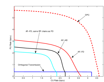
Figure 4: Rate region for AF protocol.

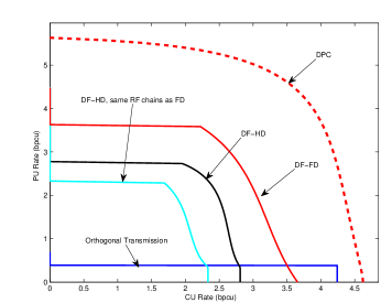
Figure 5: Rate region for DF protocol.

In Fig. 6, we plot the CU rate against the CBS power. It can be seen that the proposed FD and hybrid schemes achieve almost three times the CU rates provided by the HD mode with the same RF chains. At low SNRs, the HD mode may perform better than the FD mode while the performance gain of the FD over the HD mode is enlarged as the CBS power increases. It is also observed that the proposed hybrid schemes perform nearly as well as the best mode selection. The proposed FD and hybrid schemes achieve the same slope for the CU rate as DPC.

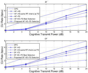
Figure 6: CU rate vs. CBS Power.

In Fig. 7, we study the impact of fixed and scalable transmit noise on the CU rate for the FD mode. It can be observed that with a fixed transmit noise power, all the achievable rates are increasing with the CBS power. The achievable rate of the AF protocol approaches that of the DF protocol at high SNRs. For the DPC scheme and the HD mode, the achievable rates saturate from $25$ dB of the CBS power, which indicates that the CBS should reserve some power in order to suppress the self-interference.

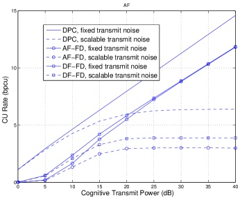
Figure 7: CU rate for both scalable and nonscalable transmit noise power.

In Fig. 8, we plot the CU rates versus the transmit noise scaling factor $\epsilon^{2}$ , when the CBS power is $20$ dB. We note that in general, FD outperforms HD even when $\epsilon^{2}$ is large, especially for the DF relaying protocol. This observation is because the transmit noise limits the performance of HD while FD can efficiently suppress the self-interference by employing optimal relay processing. As for the AF relaying protocol, the HD mode may outperform the FD mode due to the fact that the CBS amplifies the self-interference. The performance of the proposed mode selection is very close to the best selection for the AF relaying protocol; for the DF relaying protocol, they are almost identical and validate the effectiveness of the proposed selection.

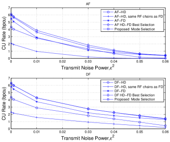
Figure 8: CU rate vs. transmit noise power.

In Fig. 9, we examine the effects of the CBS power on the PU’s outage performance. We assume the PU requires a rate of $3$ bpcu. First due to the weak primary link, the outage is almost $100\%$ if there is no assistance from the CBS. As expected, the HD mode is not efficient at low SNRs, and can even become worse than the direct transmission due to the two phases used; for AF, the outage performance is improved only when the CBS power is higher than $15$ dB, while with the same energy consumption, FD and the hybrid schemes can reduce the outage probability to $60\%$. With $25$ dB for the CBS power, AF-HD has an outage probability about $60\%$, while the hybrid schemes reduces the outage probability to below $40\%$. The FD mode with DF protocol achieves a lower saturated outage probability of $32\%$ when the CBS power is above $20$ dB.

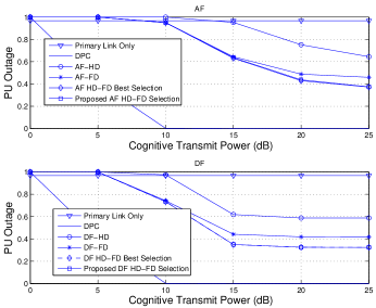
Figure 9: PU rate outage vs. CBS power.

Finally in Fig. 10, we investigate the impact of different transmit and receive antenna configurations on the FD mode, by assuming the CBS has $6$ transmit and receive RF chains. We simulate four different cases $(N_{t},N_{r})\in\{(5,1),(4,2),(3,3),(2,4)\}$. The same trends are observed for both AF and DF protocols. It can be seen that $(N_{t},N_{r})=(3,3)$ provides the best performance for medium to high SNRs; this is because the primary rate is upper bounded by the supportable rates of the PBS-CBS and CBS-PU links and therefore equal number of transmit and receive antennas is a preferred configuration. At low to medium SNRs, $(N_{t},N_{r})=(5,1)$ provides better performance than that of $(N_{t},N_{r})=(2,4)$, because the rate is limited by the CBS-PU and CBS-CU links. Therefore the CU rate takes the expression (53).

$$R_{C_{FD}}\approx\log_{2}\left(1+\frac{\max\left(0,1-\rho_{FD}^{2}-(2^{r_{0}}-1)(\epsilon^{2}+\frac{2}{P_{C}\|{\bf h}_{c0_{FD}}\|^{2}})\right)}{\epsilon^{2}+\frac{2}{P_{C}\|{\bf h}_{c_{FD}}\|^{2}}}\right).$$ (67)

It is observed that as $N_{t}$ increases, both $\|{\bf h}_{c0_{FD}}\|^{2}$ and $\|{\bf h}_{c_{FD}}\|^{2}$ increase while $\rho_{FD}^{2}$ decreases, consequently the CU rate increases as well. At high SNRs, $(N_{t},N_{r})=(2,4)$ outperforms the $(N_{t},N_{r})=(5,1)$ configuration. This is because the PBS-CBS link limits the achievable PU and CU rates and therefore more received antennas at the CBS can improve the CU rate. For the same reason, $(N_{t},N_{r})=(4,2)$ saturates when the CBS power is about $20$ dB while the performance of the case $(N_{t},N_{r})=(2,4)$ improves with the CBS power until $25$ dB.

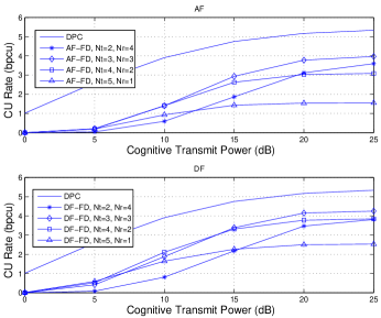
Figure 10: CU rate for different antenna configurations

VI Conclusion

We have studied the HD and the FD operation modes for the CBS in a cooperative cognitive network. We have considered transmit imperfections in both duplex modes and modeled the resulting CBS’s residual self-interference for the FD mode. Closed-form solutions or efficient 1-D search algorithms to achieve the optimal AF and DF beamforming vectors have been provided in order to characterize the achievable primary-cognitive rate regions. In addition, we proposed a hybrid scheme to switch between the HD and FD modes based on the simplified ZF beamforming design. Results have shown that the proposed FD and hybrid schemes can greatly enlarge the rate region compared to the HD mode, therefore they are introduced as efficient solutions for the active cooperation between primary and cognitive systems. The proposed cooperation substantially increases the opportunities for a CU to access the primary spectrum and improves the overall system spectral efficiency.

It is worth noting that for scenarios with a strong primary direct link, the PU receives two copies of the transmitted signal via both the direct and the relaying links by generating an artificial multipath effect. While this paper and most studies in the literature discard the direct link and only decode the relaying information, as a future direction, we can study how to efficiently combat this effect using equalization techniques [32].

Appendices

A. Proof of Theorem 1

Proof:

Without loss of generality, ${\bf A}$ can be expressed in the form of

$${\bf A} = [\bar{\bf H}~{}~{}\bar{\bf H}^{\bot}]\left[\begin{array}[]{cc}{\bf b}&{\bf C}\\ {\bf d}&{\bf E}\end{array}\right][{\bf g}^{\dagger}~{}~{}({{\bf g}^{\bot}})^{\dagger}]$$

$$= \bar{\bf H}{\bf b}{\bf g}^{\dagger}+\bar{\bf H}^{\bot}{\bf d}{\bf g}^{\dagger}+\bar{\bf H}{\bf C}({{\bf g}^{\bot}})^{\dagger}+\bar{\bf H}^{\bot}{\bf E}({{\bf g}^{\bot}})^{\dagger}$$

where $\bar{\bf H}\triangleq[{\bf h}_{c0}~{}{\bf h}_{c}]$ and ${\bf b}\in\mathbb{C}^{2\times 1},{\bf C}\in\mathbb{C}^{2\times(N-1)},{\bf d}\in\mathbb{C}^{(N-2)\times 1},{\bf E}\in\mathbb{C}^{(N-2)\times(N-1)}$ are parameter vectors and matrices.

A closer observation of the defined problem reveals that the optimization will maximize $|{\bf h}_{c0}^{\dagger}{\bf A}{\bf g}|^{2}$ while minimize $|{\bf h}_{c}^{\dagger}{\bf A}{\bf g}|^{2}$, $\|{\bf h}_{c}^{\dagger}{\bf A}\|^{2},\|{\bf h}_{c0}{\bf A}\|^{2},\|{\bf A}{\bf g}\|^{2}$ and $\|{\bf A}\|^{2}$. It is clearly seen that ${\bf C},{\bf E},{\bf d}$ do not affect the term to be maximized and setting them to be zero will help reduce the terms to be minimized, therefore ${\bf C}={\bf 0},{\bf d}={\bf 0},{\bf E}={\bf 0}$ and the optimal ${\bf A}$ has the structure of ${\bf A}=\bar{\bf H}{\bf b}{\bf g}^{\dagger}$ and can be written in a more general form of ${\bf A}={\bf w}_{a}{\bf g}^{\dagger}$ where ${\bf w}_{a}=\bar{\bf H}{\bf b}$ is a new parameter vector. ∎

B. Closed-form Solution to A General Rate Maximization Problem

Our aim here is to find the close-form solution to the rate maximization problem below:

$$\max_{{\bf w}_{1},{\bf w}_{2}} \frac{|{\bf h}_{2}^{\dagger}{\bf w}_{2}|^{2}}{1+|{\bf h}_{2}^{\dagger}{\bf w}_{1}|^{2}}$$ (71)

s.t. $$\frac{|{\bf h}_{1}^{\dagger}{\bf w}_{1}|^{2}}{1+c|{\bf h}_{1}^{\dagger}{\bf w}_{2}|^{2}}\geq\gamma_{1},|{\bf w}_{1}\|^{2}+c\|{\bf w}_{2}\|^{2}\leq P_{C},$$

where $c$ is a constant, ${\bf h}_{1},{\bf h}_{2}$ are $N\times 1$ vectors and $\gamma_{1},P_{C}$ are positive scalars. This problem has the following physical meaning. Consider a MISO broadcast system with an $N$-antenna BS and two single-antenna users. The channels from the BS to user 1 and user 2 are ${\bf h}_{1}$ and ${\bf h}_{2}$, respectively. The noise powers at users are assumed to be one, otherwise, the channel can be normalized with the noise power. Suppose the BS has a total power constraint $P_{C}$ and user 1 has a SINR constraint $\gamma_{1}$, then this problem has the interpretation of maximization of user 2’s SINR. Suppose its optimal objective value is $\gamma_{2}^{*}$. To find the optimal solution to (71), we first consider the following weighted sum power minimization problem:

$$\min_{{\bf w}_{1},{\bf w}_{2}} \|{\bf w}_{1}\|^{2}+c\|{\bf w}_{2}\|^{2}$$ (72)

s.t. $$\frac{|{\bf h}_{1}^{\dagger}{\bf w}_{1}|^{2}}{1+c|{\bf h}_{1}^{\dagger}{\bf w}_{2}|^{2}}\geq\gamma_{1},\frac{|{\bf h}_{2}^{\dagger}{\bf w}_{2}|^{2}}{1+|{\bf h}_{2}^{\dagger}{\bf w}_{1}|^{2}}\geq\gamma_{2}.$$

It can be validated that if we set $\gamma_{2}=\gamma_{2}^{*}$ in (72), then its optimal objective value is $P_{C}$ and vice versa. So we can focus on (72) in order to characterize the solution to (71). The dual problem of (72) can be derived as

$$\max_{\lambda_{1},\lambda_{2}\geq 0} \lambda_{1}+\lambda_{2}$$ (73)

s.t. $${\bf I}+\lambda_{2}{\bf h}_{2}{\bf h}_{2}^{\dagger}\succeq\frac{\lambda_{1}}{\bar{\gamma}_{1}}{\bf h}_{1}{\bf h}_{1}^{\dagger},\bar{\gamma}_{1}\triangleq c\gamma_{1}$$

$${\bf I}+\lambda_{1}{\bf h}_{1}{\bf h}_{1}^{\dagger}\succeq\frac{\lambda_{2}}{\gamma_{2}}{\bf h}_{1}{\bf h}_{2}^{\dagger},$$

where $\lambda_{1}$ and $\lambda_{2}$ are dual variables. The two linear matrix inequality constraints uniquely determine $\lambda_{1}$ and $\lambda_{2}$:

$$\lambda_{1} = \frac{\bar{\gamma}_{1}}{{\bf h}_{1}^{\dagger}\left({\bf I}+\lambda_{1}\bar{\bf h}_{2}{\bf h}_{2}^{\dagger}\right)^{-1}{\bf h}_{1}},\lambda_{2} = \frac{\gamma_{2}}{{\bf h}_{2}^{\dagger}\left({\bf I}+\lambda_{1}{\bf h}_{1}{\bf h}_{1}^{\dagger}\right)^{-1}{\bf h}_{2}}.$$ (74)

Using matrix inversion lemma and define $\rho^{2}\triangleq\frac{|{\bf h}_{1}^{\dagger}{\bf h}_{2}|^{2}}{\|{\bf h}_{1}\|^{2}\|{\bf h}_{2}\|^{2}}$ we have

$$\lambda_{1} = \frac{\bar{\gamma}_{1}(1+\lambda_{2}\|{\bf h}_{2}\|^{2})}{\|{\bf h}_{1}\|^{2}+\lambda_{2}(\|{\bf h}_{2}\|^{2}\|{\bf h}_{1}\|^{2}-\|{\bf h}_{2}^{\dagger}{\bf h}_{1}\|^{2})}$$ (75)

$$= \frac{\bar{\gamma}_{1}(1+\lambda_{2}\|{\bf h}_{2}\|^{2})}{\|{\bf h}_{1}\|^{2}(1+\lambda_{2}\|{\bf h}_{2}\|^{2}(1-\rho^{2}))},$$

$$\lambda_{2} = \frac{\gamma_{2}(1+\lambda_{1}\|{\bf h}_{1}\|^{2})}{\|{\bf h}_{2}\|^{2}+\lambda_{1}(\|{\bf h}_{2}\|^{2}\|{\bf h}_{1}\|^{2}-\|{\bf h}_{2}^{\dagger}{\bf h}_{1}\|^{2})}$$

$$= \frac{\gamma_{2}(1+\lambda_{1}\|{\bf h}_{1}\|^{2})}{\|{\bf h}_{2}\|^{2}(1+\lambda_{1}\|{\bf h}_{1}\|^{2}(1-\rho^{2}))}.$$

Remember we also have a power equation below:

$$\lambda_{1}+\lambda_{2}=P_{C}.$$ (76)

It is observed that $\lambda_{1},\lambda_{2},\gamma_{2}$ should satisfy and uniquely determined by the above three equations (75-76), so the analytical solutions can be found. Define $A=\|{\bf h}_{1}\|^{2}\|{\bf h}_{2}\|^{2}(1-\rho^{2}),B=-(\|{\bf h}_{2}\|^{2}\bar{\gamma}_{1}+P_{C}\|{\bf h}_{1}\|^{2}\|{\bf h}_{2}\|^{2}(1-\rho^{2})+\|{\bf h}_{1}\|^{2})$, and $C=(P_{C}\|{\bf h}_{2}\|^{2}+1)\bar{\gamma}_{1}$. Then from (75), we have

$$f(\lambda_{1})\triangleq A\lambda_{1}^{2}+B\lambda_{1}+C=0.$$ (77)

Since $A>0,C>0,B<0$, $f(\lambda)=0$ has positive two roots. Because $f(P_{C})<0$, we know that the optimal $\lambda_{1}$ corresponds to the minimum root. Once $\lambda_{1}$ is found, $\lambda_{2}$ and $\gamma_{2}$ can be easily derived from (75-76).

References

• [1] A.K. Sadek, K.J.R. Liu, and A. Ephremides, “Cognitive multiple access via cooperation: Protocol design and stability analysis,” IEEE Trans. Inf. Theory, vol. 53, no. 10, pp. 3677-3696, Oct. 2007.
• [2] O. Simeone, Y. Bar-Ness and U. Spagnolini, “Stable throughput of cognitive radios with and without relaying capability,” IEEE Trans. Commun., vol. 55, no. 12, pp. 2351-2360, Dec. 2007.
• [3] O. Simeone, I. Stanojev, S. Savazzi, Y. Bar-Ness, U. Spagnolini, and R. Pickholtz, “Spectrum leasing to cooperating secondary ad hoc networks,” IEEE J. Sel. Areas Commun., vol. 26, no. 1, pp. 203 -213, Jan. 2008.
• [4] W. Su, J. Matyjas, and S. Batalama, “Active cooperation between primary users and cognitive radio users in cognitive ad-hoc networks,” in Proc. IEEE ICASSP, Dallas, TX. Mar. 2010, pp. 3174-3177.
• [5] K. Hamdi, K. Zarifi, K. B. Letaief, and A. Ghrayeb, “Beamforming in relay-assisted cognitive radio systems: A convex optimization approach,” in Proc. IEEE Int. Conf. Commun. (ICC), Kyoto, Japan, 5-9 June 2011, pp. 1-5.
• [6] S.H. Song and K. B. Letaief, “Prior zero-forcing for relaying primary signals in cognitive network,“ in Proc. IEEE Global Commun. Conf. (GLOBECOM), Dec. 05-09, 2011, pp. 1-5.
• [7] G. Zheng, S.H. Song, K. K. Wong, and B. Ottersten, “Cooperative cognitive networks: Optimal, distributed and low-complexity algorithms,” submitted to IEEE Trans. Signal Process., [Online]. Available: http://arxiv.org/abs/1204.2651.
• [8] B. P. Day, A. R. Margetts, D. W. Bliss, and P. Schniter, “Full-duplex bidirectional MIMO: Achievable rates under limited dynamic range,” IEEE Trans. Signal Process., vol. 60, no. 7, pp. 3702-3713, July 2012.
• [9] T. Riihonen, S. Werner, R. Wichman, and E. Zacarias B., “On the feasibility of full-duplex relaying in the presence of loop interference,” in 10th IEEE Workshop Signal Process. Advances Wireless Commun. (SPAWC), Perugia, Italy, June 2009, pp. 275-279.
• [10] M. Duarte and A. Sabharwal, “Full-duplex wireless communications using off-the-shelf radios: Feasibility and first results,” in 44th Annual Asilomar Conf. Signals, Syst., Comput., Pacific Grove, CA, Nov. 2010, pp. 1558-1562.
• [11] A. Sahai, G. Patel, and A. Sabharwal, “Pushing the limits of full-duplex: Design and real-time implementation,” Rice University Technical Report TREE1104, June 2011, [Online]. Available: http://arxiv.org/abs/1107.0607.
• [12] T. Riihonen, S. Werner, and R. Wichman, “Transmit power optimization for multiantenna decode-and-forward relays with loopback self-interference from full-duplex operation,” in 45th Annual Asilomar Conf. Signals, Syst., Comput., Pacific Grove, CA, Nov. 2011, pp. 1408-1412.
• [13] T. Riihonen, S. Werner, and R. Wichman, “Mitigation of loopback self-interference in full-duplex mimo relays,” IEEE Trans. Signal Process., vol. 59, no. 12, pp. 5983-5993, Dec. 2011.
• [14] B. P. Day, A. R. Margetts, D. W. Bliss, and P. Schniter, “Full-duplex MIMO relaying: achievable rates under limited dynamic range,” IEEE J. Sel. Areas Commun., vol. 30 , no. 8, pp. 1541-1553, Sept. 2012.
• [15] T. Riihonen, S. Werner, and R. Wichman, “Hybrid full-duplex/half-duplex relaying with transmit power adaptation,” IEEE Trans. Wireless Commun., vol. 10, no. 9, pp. 3074-3085, Sept. 2011.
• [16] I. Krikidis, H. A. Suraweera, P. J. Smith, and C. Yuen, “Full-duplex relay selection for amplify-and-forward cooperative networks,” IEEE Trans. Wireless Commun., vol. 11, pp. 4381–4393, Dec. 2012.
• [17] N. Devroye, P. Mitran, and V. Tarokh, “Achievable rates in cogtive radio channels,” IEEE Trans. Inf. Theory, vol. 52, pp. 1813-1827, May 2006.
• [18] S. Srinivasa, and Syed A. Jafar, “The throughput potential of cognitive radio-a theoretical perspective,” IEEE Commun. Mag., vol. 45, no. 5, pp. 73-79, May 2007.
• [19] A. Jovicic and P. Viswanath, “Cognitive radio: An information-theoretic perspective,” IEEE Trans. Inf. Theory, vol. 55, no. 9, pp. 3945–3958, Sept. 2009.
• [20] H. Yu, Y. Sung and Y. H. Lee, “Superposition data transmission for cognitive radios: Performance and algorithms,” in Proc. IEEE Military Commun. Conf. (MILCOM), San Diego, USA, 16-19 Nov. 2008, pp. 1-6.
• [21] K. K. Wong, “Maximizing the sum-rate and minimizing the sum-power of a broadcast 2-user 2-input multiple-output antenna system using a generalized zeroforcing approach,” IEEE Trans. Wireless Commun., vol. 5, no. 12, pp. 3406-3412, Dec. 2006.
• [22] B. Chen and M. J. Gans, “MIMO communications in ad hoc networks,” IEEE Trans. Sig. Proc., vol. 54, no. 7, pp. 2773-2783, July 2006.
• [23] S.-J. Kim, and G. B. Giannakis, “Optimal resource allocation for MIMO ad hoc cognitive radio networks,” IEEE Trans. Inf. Theory, vol. 57, no. 5, pp. 3117-3131, May 2011.
• [24] M. Duarte, A. Sabharwal, V. Aggarwal, R. Jana, K. K. Ramakrishnan, C. Rice and N. K. Shankaranarayanan, “Design and characterization of a full-duplex multi-antenna system for WiFi networks,” submitted to IEEE Trans. Veh. Tech., Oct 2012, [Online]. Available: http://arxiv.org/abs/1210.1639.
• [25] H. Ju, E. Oh, and D. Hong, “Catching resource-devouring worms in next-generation wireless relay systems: Two-way relay and full-duplex relay,” IEEE Commun. Mag., vol. 47, no. 9, pp. 58-65, Sept. 2009.
• [26] G. Fettweis, M. Lohning, D. Petrovic, M. Windisch, P. Zillmann, and W. Rave, “Dirty RF: A New Paradigm,” in Proc. IEEE Int. Symp. Personal, Indoor Mobile Radio Commun. (PIMRC), pp. 2347-2355, Berlin, Germany, Sept. 11-14, 2005, pp. 2347-2355.
• [27] C. Shin, R.W. Heath, and E.J. Powers, “Blind channel estimation for MIMO-OFDM systems,” IEEE Trans. Veh. Technol., vol. 56, no. 2, pp. 670-685, Mar. 2007.
• [28] O. Simeone, Y. Bar-Ness and U. Spagnolini, “Stable throughput of cognitive radios with and without relaying capability,” IEEE Trans. Commun., vol. 55, no. 12, pp. 2351-2360, Dec. 2007.
• [29] I. Krikidis, N. Devroye, and J. Thompson, “Stability analysis for cognitive radio with multi-access primary transmission,” IEEE Trans. Wireless Commun., vol. 9, no. 1, pp. 72-77, Jan. 2010.
• [30] A. Bletsas, A. Khisti, D. P. Reed, A. Lippman, “A simple cooperative diversity method based on network path selection,” IEEE J. Sel. Areas Commun., vol. 24, no. 3, pp. 659-672, Mar. 2006.
• [31] H. A. Suraweera, P. J. Smith, A. Nallanathan, and J. S. Thompson, “Amplify-and-forward relaying with optimal and suboptimal transmit antenna selection,” IEEE Trans. Wireless Commun., vol. 10, pp. 1874-1885, June 2011.
• [32] T. M. Kim and A. Paulraj, “Outage probability of amplify-and-forward cooperation with full duplex relay,” in Proc. IEEE Wireless Commun. Netw. Conf. (WCNC), Paris, France, 1-4 Apr. 2012, pp. 75-79.