An alternative realization of spontaneous emission cancellation via Field Generated Coherence (FGC)

Abstract

In contrast to the traditional Spontaneous Generated Coherence (SGC), Field Generated Coherence (FGC)-based atomic scheme is presented for spontaneous emission cancellation. It is easy to achieve externally controllable experimental trapping condition in this 4-field-driven 5-level atomic system. Consequently, due to the FGC the decay from the central dressed bare-energy-state of the set of upper three closely spaced hyperfine decaying states of Sodium D2 line is completely cancelled under the trapping condition, exhibiting a novel phenomenon of a dark bare-energy-state. Extending to an atomic system of simple probability loss, based on Sodium D1 line, the bright atom can also be darkened under its trapping condition, representing another experimentally viable, novel and interesting phenomenon.

Date text]date

The interaction of atoms or molecules with the environmental modes leads to spontaneous emission in atomic systems. The simplest example is the free space where atomic coherence and quantum interference are the basic mechanisms for cancellation Agarwal ; Alzetta ; Gray of spontaneous emission, a basic phenomenon not questionable regarding its utilities Garraway ; Zhu ; Kochar ; Scully . On the basis of its mechanisms we can divide it into two main categories. The first is spontaneous emission generated coherence (SGC) where the decay processes generate coherence among themselves to cancel spontaneous emission Zhu-Scully ; Paspalakis . The second mechanism depends on the driving fields itself where one coherence induces the others. This is intuitively the simplest mechanism which may be easily realized in a laboratory, and is the subject of this letter. We introduce a system based on Fields Generated Coherence (FGC), a collective coherence effect of amplitudes and phases of the driving fields on the spontaneous emission processes. Spontaneous emission can be cancelled under a field-dependent trapping condition along with the other atomic population transfer effects among the three decaying dressed bare-energy-states making the central one completely dark, an unexpected but viably novel phenomenon. Remarkably, the trapping condition achieved for this system is externally controllable and easy to implement experimentally. Furthermore, the same concept can be extended to an atomic system of simple probability loss adjustable with a recent experiment to darken the brightened atom. This is an amazing and interesting phenomenon leading to the trapping of all the population in the unique excited decaying bare-energy-state. Generally, all population in this one-atom quantum system may be transferred into a unique, extremely slowly decaying dressed state, allowing effective storage and manipulation of atomic population like in Ref. 2-atom but with the additional darkened bare-energy-state. It is worthwhile to note the confusion of the terminology in literature between the control and cancellation Paspalakis of spontaneous emission which needs clarification F-Ghafoor .

Prior to discussing the physics of the FGC regarding the spontaneous emission cancellation in our proposed scheme, let us recall briefly some pioneer works carried out in the area of SGC and its complications. For example, Zhu and Scully Zhu-Scully observed spectral line elimination associated with dressed state in a four-level atomic system, arising due to quantum interference effect between the upper decaying non-degenerate two levels to the same lower level. Further, Paspalakis and Knight proposed a phase control scheme in a four-level atom driven by two lasers of the same frequency Paspalakis , where the relative phase of the two lasers was used to get extreme line-width narrowing, partial control of all the three dressed-state and total cancellation of a dressed-state in the spontaneous emission spectrum. The beautiful physics of these processes is also explained in Ref. Hwang-Zhu by using dressed state-vector approach. However, all the spontaneous emission cancellation schemes have one common origin, that is, the decay processes from two closely spaced atomic levels to a third level with a condition of parallel dipole moments. Two closely spaced levels can hardly be created by mixing two-parity levels due to static electric field. For example, a separation of even 40$\gamma$ for $\left|2s\right\rangle$ and $\left|2p\right\rangle$ states of hydrogen atom Hakuta could not utilized for successful demonstration of the processes. It is hard to satisfy simultaneously the rigorous condition for the spontaneously generated coherence of nearly degenerate levels and the parallel dipole moments. Consequently, some experiments have been performed (see Ref. Xia ) but with a doubt, as commented upon in Ref. Li . Ultimately, a scheme based on orthogonal dipole moments F-Ghafoor ; Ghafoor00 may lead to experimentally more realistic system if it qualifies for spontaneous emission cancellation under a viably novel phenomenon. In the following this approach is developed.

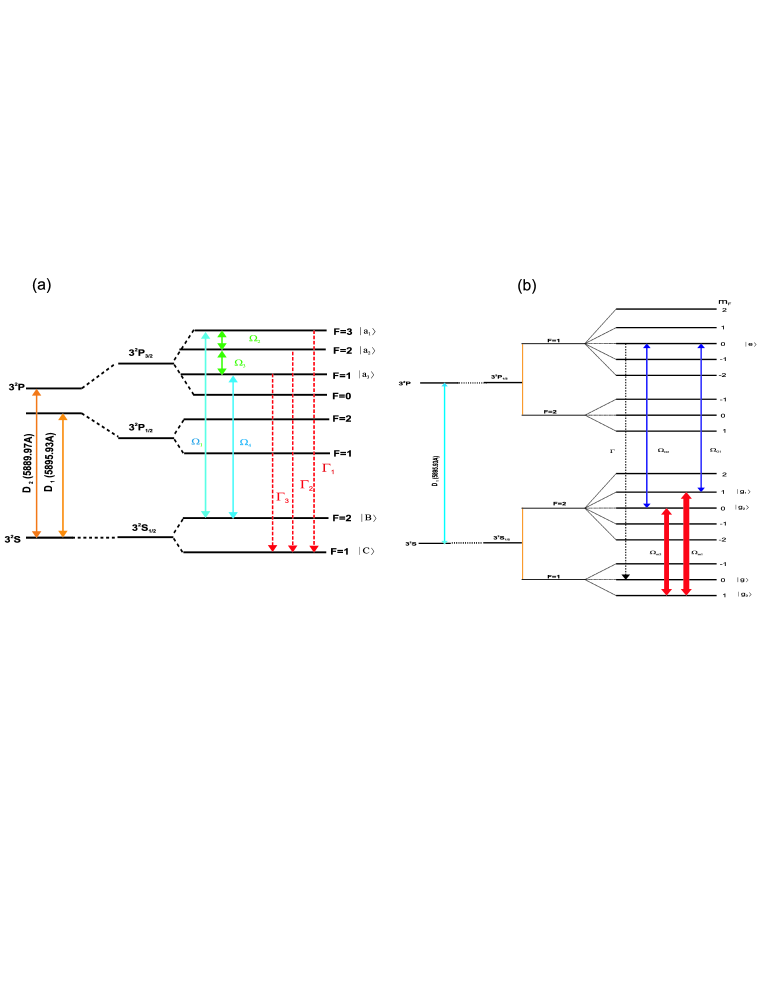
Figure 1: Schematics (a) Hyperfine-structured Sodium D2 line. (b): Zeeman-structured Sodium D1 line

Consider a 5-level atomic system based on the hyperfine-structured Sodium D2 line (3S${}_{1/2}^{2}\Longleftrightarrow$3P${}_{3/2}^{2}$) [see Fig. 1(a)]. Two pairs of 3²P${}_{3/2},$F=1 ($\left|a_{3}\right\rangle$), 3²P${}_{3/2},$F=2 ($\left|a_{2}\right\rangle$), 3²P${}_{3/2},$F=3 ($\left|a_{1}\right\rangle$) from the excited quadruplet are driven by microwave fields to have the Rabi-frequencies $\Omega_{1}$ and $\Omega_{2}$ respectively. The ground state 3²S${}_{1/2},$F=2 ($\left|B\right\rangle$) is coupled with the excited states $\left|a_{1}\right\rangle$ and $\left|a_{3}\right\rangle$ via two coherent fields to have Rabi frequencies $\Omega_{3}$ and $\Omega_{4\text{ }}$ respectively. The selected three closely spaced states decay to another ground state 3²S${}_{1/2},$F=1 ($\left|C\right\rangle$) (allowed transitions) by the vacuum field modes couplings. Now we have to measure the spectrum in steady state limit. Furthermore, the experiment of Xia et al. Xia using sodium dimer may also be adjusted with this set-up using the naturally existing series of coupled excited energy states arising due to mixing of the triplet and singlet g-parity Rydberg states by the spin-orbit coupling known as occasional perturbation Herz ; Wang .

Using the Weisskofp-Wigner theory the equations of motion for the probability amplitudes of the atomic system are obtained as

$$\overset{\cdot}{A}_{1}\left(t\right) =-i\Omega_{2}e^{i\Delta_{2}t}A_{2}\left(t\right)-i\Omega_{1}e^{i\Delta_{1}t}B\left(t\right)-\frac{\Gamma_{1}}{2}A_{1}\left(t\right)$$

$$-p_{1}\frac{\sqrt{\Gamma_{1}\Gamma_{2}}}{2}e^{-i\omega_{12}t}A_{2}\left(t\right)-p_{2}\frac{\sqrt{\Gamma_{1}\Gamma_{3}}}{2}e^{-i\omega_{13}t}A_{3}\left(t\right),$$ (1)

$$\overset{\cdot}{A}_{2}\left(t\right) =-i\Omega_{2}^{\ast}e^{-i\Delta_{2}t}A_{1}\left(t\right)-i\Omega_{3}e^{i\Delta_{3}t}A_{3}\left(t\right)-\frac{\Gamma_{2}}{2}A_{2}\left(t\right)$$

$$-p_{1}\frac{\sqrt{\Gamma_{1}\Gamma_{2}}}{2}e^{-i\omega_{12}t}A_{1}\left(t\right)-p_{3}\frac{\sqrt{\Gamma_{2}\Gamma_{3}}}{2}e^{-i\omega_{23}t}A_{3}\left(t\right),$$ (2)

$$\overset{\cdot}{A}_{3}\left(t\right) =-i\Omega_{3}^{\ast}e^{-i\Delta_{3}t}A_{2}\left(t\right)-i\Omega_{2}e^{i\Delta_{4}t}B\left(t\right)-\frac{\Gamma_{3}}{2}A_{3}\left(t\right)$$

$$-p_{2}\frac{\sqrt{\Gamma_{1}\Gamma_{3}}}{2}e^{-i\omega_{13}t}A_{1}\left(t\right)-p_{3}\frac{\sqrt{\Gamma_{2}\Gamma_{3}}}{2}e^{-i\omega_{23}t}A_{2}\left(t\right),$$ (3)

$$\overset{\cdot}{B}\left(t\right) =-i\Omega_{1}^{\ast}e^{-i\Delta_{1}t}A_{1}\left(t\right)-i\Omega_{4}^{\ast}e^{-i\Delta_{4}t}A_{3}\left(t\right),$$ (4)

$$\overset{\cdot}{C_{k}}\left(t\right) =-ig_{\mathbf{k}}^{\ast(1)}e^{-i\delta_{1}t}A_{1}\left(t\right)-ig_{\mathbf{k}}^{\ast(2)}e^{-i\delta_{2}t}A_{2}\left(t\right)-ig_{\mathbf{k}}^{\ast(3)}e^{-i\delta_{3}t}A_{3}\left(t\right),$$ (5)

where $\Gamma_{j}$ $\left(j=1,2,3\right)$ are the radiative decay rates from the upper three levels to the ground level, respectively. Further $\Delta_{1}=\omega_{a_{1}}-\omega_{b}-\upsilon_{1},$ $\Delta_{2}=\omega_{a_{1}}-\omega_{a_{2}}-\upsilon_{2},$ $\Delta_{3}=$ $\omega_{a_{2}}-\omega_{a_{3}}-\upsilon_{3},$ and $\Delta_{4}=\omega_{a_{3}}-\omega_{b}-\upsilon_{4}$ are the driving fields detunings, $\delta_{1}=\omega_{a_{1}}-\omega_{c}-\upsilon_{\mathbf{k}},$ $\delta_{2}=\omega_{a_{2}}-\omega_{c}-\upsilon_{\mathbf{k}},$ and $\delta_{3}=\omega_{a_{3}}-\omega_{c}-\upsilon_{\mathbf{k}},$ are the vacuum fields detunings while $g_{\mathbf{k}}^{\left(1\right)},$ $g_{\mathbf{k}}^{\left(2\right)}$ and $g_{\mathbf{k}}^{\left(3\right)}$ are the vacuum field coupling constants, respectively. However, the alignments $p_{i}=\mathbf{r}_{a_{i},c}.\mathbf{r}_{a_{j},c}/r_{a_{i},c}r_{a_{j},c}$ $\vee$ $(i=1-3$ $\&$ $j=i)$ of the matrix elements among the three dipole moments are neglecting under the approximations $\omega_{12},$ $\omega_{23}\gg\Gamma_{1,2,3}$ F-Ghafoor ; Ghafoor00 .

Using Laplace transforms and the final value theorem along with choosing the detuning parameters $\delta_{i}$ $\left(i=1-3\right)=$ $\delta+\omega_{12},$ $\delta,$ $\delta-\omega_{12}$ $\vee$ $\delta=\omega_{a_{2}c}-\nu_{k}$ and $\omega_{12}\approx\omega_{23},$ the steady state probability amplitudes are given by

$$\mathcal{A}_{1}\left(\delta+\omega_{12}\right) =\frac{\mathcal{A}_{1}\left(0\right)}{\mathcal{D}\left(\delta+\omega_{12}\right)}[i\left(\delta+\omega_{12}\right)[i\left(\delta+\omega_{12}\right)+\frac{\Gamma_{2}}{2}][i\left(\delta+\omega_{12}\right)+\frac{\Gamma_{3}}{2}]$$

$$+[i\left(\delta+\omega_{12}\right)+\frac{\Gamma_{2}}{2}]\left|\Omega_{4}\right|^{2}+i\left(\delta+\omega_{12}\right)\left|\Omega_{3}\right|^{2}]$$

$$+\frac{\mathcal{A}_{2}\left(0\right)}{\mathcal{D}\left(\delta+\omega_{12}\right)}\left[\left(\delta+\omega_{12}\right)\left[i\left(\delta+\omega_{12}\right)+\frac{\Gamma_{3}}{2}\right]\Omega_{2}-i\Omega_{2}\left|\Omega_{4}\right|^{2}+i\Omega_{1}\Omega_{3}^{\ast}\Omega_{4}^{\ast}\right]$$

$$-\frac{\mathcal{A}_{3}\left(0\right)}{\mathcal{D}\left(\delta+\omega_{12}\right)}\left[i\left(\delta+\omega_{12}\right)\Omega_{2}\Omega_{3}+\left[i\left(\delta+\omega_{12}\right)+\frac{\Gamma_{2}}{2}\right]\Omega_{1}\Omega_{4}^{\ast}\right]$$

$$+i\frac{\mathcal{B}\left(0\right)}{\mathcal{D}\left(\delta+\omega_{12}\right)}\left[\Omega_{2}\Omega_{3}\Omega_{4}-\left[i\left(\delta+\omega_{12}\right)+\frac{\Gamma_{3}}{2}\right]\left[i\left(\delta+\omega_{12}\right)+\frac{\Gamma_{2}}{2}\right]\Omega_{1}-\Omega_{1}\left|\Omega_{3}\right|^{2}\right],$$ (6)

$$\mathcal{A}_{2}\left(\delta\right) =i\frac{\mathcal{A}_{1}\left(0\right)}{\mathcal{D}\left(\delta\right)}\left[-i\delta\left(i\delta+\frac{\Gamma_{3}}{2}\right)\Omega_{2}^{\ast}+\Omega_{2}^{\ast}\left|\Omega_{4}\right|^{2}-\Omega_{1}^{\ast}\Omega_{3}\Omega_{4}\right]$$

$$-\frac{\mathcal{A}_{2}\left(0\right)}{\mathcal{D}\left(\delta\right)}\left[i\delta\left(i\delta+\frac{\Gamma_{1}}{2}\right)\left(i\delta+\frac{\Gamma_{3}}{2}\right)+\left(i\delta+\frac{\Gamma_{1}}{2}\right)\left|\Omega_{4}\right|^{2}+\left(i\delta+\frac{\Gamma_{3}}{2}\right)\left|\Omega_{1}\right|^{2}\right]$$

$$+i\frac{\mathcal{A}_{3}\left(0\right)}{\mathcal{D}\left(\delta\right)}\left[-\Omega_{1}\Omega_{2}^{\ast}\Omega_{4}^{\ast}-i\delta\left(i\delta+\frac{\Gamma_{1}}{2}\right)\Omega_{3}-\Omega_{3}\left|\Omega_{1}\right|^{2}\right]$$

$$-\frac{\mathcal{B}\left(0\right)}{\mathcal{D}\left(\delta\right)}\left[\left(i\delta+\frac{\Gamma_{1}}{2}\right)\Omega_{3}\Omega_{4}+\left(i\delta+\frac{\Gamma_{3}}{2}\right)\Omega_{1}\Omega_{2}^{\ast}\right],$$ (7)

and

$$\mathcal{A}_{3}\left(\delta-\omega_{12}\right) =\frac{\mathcal{A}_{1}\left(0\right)}{\mathcal{D}\left(\delta-\omega_{12}\right)}\left[i\left(\delta-\omega_{12}\right)\Omega_{2}^{\ast}\Omega_{3}^{\ast}-[i\left(\delta-\omega_{12}\right)+\frac{\Gamma_{2}}{2}]\Omega_{1}^{\ast}\Omega_{4}\right]$$

$$+i\frac{\mathcal{A}_{2}\left(0\right)}{\mathcal{D}\left(\delta-\omega_{12}\right)}\left[i\left(\delta-\omega_{12}\right)[i\left(\delta-\omega_{12}\right)+\frac{\Gamma_{1}}{2}]\Omega_{3}^{\ast}-\Omega_{1}^{\ast}\Omega_{2}\Omega_{4}+\Omega_{1}^{\ast}\Omega_{1}\Omega_{3}^{\ast}\right]$$

$$-\frac{\mathcal{A}_{3}\left(0\right)}{\mathcal{D}\left(\delta-\omega_{12}\right)}[i\left(\delta-\omega_{12}\right)[i\left(\delta-\omega_{12}\right)+\frac{\Gamma_{1}}{2}][i\left(\delta-\omega_{12}\right)+\frac{\Gamma_{2}}{2}]$$

$$+[i\left(\delta-\omega_{12}\right)+\frac{\Gamma_{2}}{2}]\left|\Omega_{1}\right|^{2}+i\left(\delta-\omega_{12}\right)\left|\Omega_{2}\right|^{2}]$$

$$+i\frac{\mathcal{B}\left(0\right)}{\mathcal{D}\left(\delta-\omega_{12}\right)}\left[-\Omega_{1}\Omega_{2}^{\ast}\Omega_{3}^{\ast}-\left[i\left(\delta-\omega_{12}\right)+\frac{\Gamma_{1}}{2}\right]\left[i\left(\delta-\omega_{12}\right)+\frac{\Gamma_{2}}{2}\right]\Omega_{4}-\Omega_{4}\left|\Omega_{2}\right|^{2}\right].$$ (8)

Herein

$$\mathcal{D}\left(\delta\pm\omega_{12}\right),(\delta) =\left(\delta\pm\omega_{12}\right)^{4},\delta^{4}-i(\frac{\Gamma_{1}}{2}+\frac{\Gamma_{2}}{2}+\frac{\Gamma_{3}}{2})\left(\delta\pm\omega_{12}\right)^{3},\delta^{3}$$

$$-(\frac{\Gamma_{1}\Gamma_{3}}{4}+\frac{\Gamma_{2}\Gamma_{3}}{4}+\frac{\Gamma_{1}\Gamma_{2}}{4}+\sum_{i=1}^{4}\left|\Omega_{i}\right|^{2})\left(\delta\pm\omega_{12}\right)^{2},\delta^{2}$$

$$+i[\frac{\Gamma_{1}\Gamma_{2}\Gamma_{3}}{8}+(\frac{\Gamma_{1}}{2}+\frac{\Gamma_{2}}{2})\left|\Omega_{4}\right|^{2}+\frac{\Gamma_{1}}{2}\left|\Omega_{3}\right|^{2}+\frac{\Gamma_{3}}{2}\left|\Omega_{2}\right|^{2}$$

$$+(\frac{\Gamma_{2}}{2}+\frac{\Gamma_{3}}{2})\left|\Omega_{1}\right|^{2}]\left(\delta\pm\omega_{12}\right),\delta+(\frac{\Gamma_{1}\Gamma_{2}}{4}\left|\Omega_{4}\right|^{2}+\frac{\Gamma_{2}\Gamma_{3}}{4}\left|\Omega_{1}\right|^{2}$$

$$+\left|\Omega_{2}\right|^{2}\left|\Omega_{4}\right|^{2}+\left|\Omega_{1}\right|^{2}\left|\Omega_{3}\right|^{2}-\Omega_{1}^{\ast}\Omega_{2}\Omega_{3}\Omega_{4}+\Omega_{1}\Omega_{2}^{\ast}\Omega_{3}^{\ast}\Omega_{4}^{\ast}).$$ (9)

The spontaneous emission spectrum for the atom initially in $\left|B\right\rangle$ can then be calculated analytically from $\mathbb{S(\delta)}=\Gamma_{n}\left|C_{k}\left(t\longrightarrow\infty\right)\right|^{2}/2\pi\left|g_{k}^{(n)}\right|^{2},$ $\left(n=1-3\right)$. Further, to interpret the result we can write $C_{k}\left(t\rightarrow\infty\right)$ as F-Ghafoor

$$C_{k}\left(t\rightarrow\infty\right) \varpropto\sum_{i=1}^{4}\frac{g_{k}^{\ast}}{\boldsymbol{\digamma}_{1}}\left[\frac{\left[\Omega_{2}\Omega_{3}\Omega_{4}-\left[i\left(\lambda_{i}+\omega_{12}\right)+\frac{\Gamma_{3}}{2}\right]\left[i\left(\lambda_{i}+\omega_{12}\right)+\frac{\Gamma_{2}}{2}\right]\Omega_{1}-\Omega_{1}\left|\Omega_{3}\right|^{2}\right]\Bbbk_{i}}{\Delta-\lambda_{i}}\right]$$

$$+\sum_{i=1}^{4}\frac{g_{k}^{\ast}}{\boldsymbol{\digamma}_{2}}\left[\frac{\left[\left(i\mu_{i}+\frac{\Gamma_{1}}{2}\right)\Omega_{2}\Omega_{3}+\left(i\mu_{i}+\frac{\Gamma_{3}}{2}\right)\Omega_{1}\Omega_{2}^{\ast}\right]\mathbb{R}_{i}}{\Delta-\mu_{i}}\right]$$

$$+\sum_{i=1}^{4}\frac{g_{k}^{\ast}}{\boldsymbol{\digamma}_{3}}\left[\frac{\left[-\Omega_{1}\Omega_{2}^{\ast}\Omega_{3}^{\ast}-\left[i\left(\kappa_{i}-\omega_{12}\right)+\frac{\Gamma_{1}}{2}\right]\left[i\left(\kappa_{i}-\omega_{12}\right)+\frac{\Gamma_{2}}{2}\right]\Omega_{4}-\Omega_{4}\left|\Omega_{2}\right|^{2}\right]\mathbb{C}_{i}}{\Delta-\kappa_{i}}\right]$$ (10)

where, $\boldsymbol{\digamma}_{j}$ $\left(j=1-3\right)=R_{1}^{3}(R_{3}-R_{4})(R_{2}^{2}+R_{3}R_{4}-2R_{2}\lambda_{4})+R_{2}^{3}[(R_{4}-R_{3})(R_{1}^{2}+R_{3}R_{4})-R_{1}(R_{4}^{2}-R_{3}^{2})]+R_{3}^{3}(R_{4}-R_{1})[R_{1}R_{4}-R_{2}(R_{4}-R_{2})]+R_{4}^{3}[(R_{3}-R_{1})(R_{1}^{2}-R_{1}R_{2}-R_{2}^{2})+R_{2}(R_{4}^{2}-R_{1}^{2})]+R_{1}R_{2}R_{3}R_{4}[R_{1}(1+R_{4})-2R_{3}R_{4}],$ with $R^{\prime}s$ $\Longrightarrow\lambda_{i},$ $\mu_{i},$ $\kappa_{i}$ for each term being the roots of quartet Eqs. (9), respectively. Also $M_{j}\left(1-3\right)=\sum\limits_{i=1}^{4}\Bbbk_{i},\mathbb{R}_{i},\mathbb{C}_{i}=(R_{2}^{2}+R_{3}R_{4})(R_{4}-R_{3})-R_{2}(R_{4}^{2}-R_{3}^{2}),$ $(R_{3}^{2}+R_{4}R_{1})(R_{1}-R_{4})-R_{3}(R_{1}^{2}-R_{4}^{2}),$ $(R_{4}^{2}+R_{1}R_{2})(R_{2}-R_{1})-R_{4}(R_{2}^{2}-R_{1}^{2}),$ $(R_{1}^{2}+R_{2}R_{3})(R_{3}-R_{2})-R_{1}(R_{3}^{2}-R_{2}^{2}).$ Further, the phases associated with the two microwave fields are $\Omega_{2}=$ $\left|\Omega_{2}\right|e^{i\varphi_{2}}$ and $\Omega_{3}=\left|\Omega_{3}\right|e^{i\varphi_{3}}$ while $\Omega_{1}=\left|\Omega_{1}\right|$ and $\Omega_{4}=\left|\Omega_{4}\right|$ are real. The spontaneous emission spectrum $\mathbb{S(\delta)}$ for any values of spectroscopic parameters is then given by

$$\mathbb{S(\delta)}=\Gamma_{1}\left|\sum_{i=1}^{4}\frac{\chi_{i}+i\tau_{i}}{\left(\delta-\varrho_{i}\right)+i\sigma_{i}}\right|^{2}+\Gamma_{2}\left|\sum_{i=1}^{4}\frac{\gamma_{i}+i\varpi_{i}}{\left(\delta-\sigma_{i}\right)+i\theta_{i}}\right|^{2}+\Gamma_{3}\left|\sum_{i=1}^{4}\frac{\epsilon_{i}+i\varepsilon_{i}}{\left(\delta-\eta_{i}\right)+i\rho_{i}}\right|^{2},$$ (11)

where all the symbols appear for appropriate integers associated with a chosen set of spectroscopic parameters of the system. Now, Eq. (11) consists of three parts where every ones is associated with four dressed-states. Here we neglected the interference terms among the three sets of dressed-states due to large separation among the bare-state. Therefore, the spectrum consists, in general of twelve peaks located at $\delta=\rho_{i}$, $\sigma_{i}$ and $\theta_{i}$ with the peak heights ($\chi_{i}^{2}+\tau_{i}^{2})/\varrho_{i}^{2},$ ($\gamma_{i}^{2}+\varpi_{i}^{2})/\sigma_{i}^{2}$ and ($\epsilon_{i}^{2}+\varepsilon_{i}^{2})/\eta_{i}^{2}$ (for $i=1-4$), respectively.

Next, I examine the condition for a trapping state in this system for SGC and set the constant part of the characteristics equation to zero. The resulting trapping condition when satisfy the equation, $(\Gamma_{1}\Gamma_{2}/2+\Gamma_{2}\Gamma_{3}/2+4\left|\Omega\right|)-i\left(4\left|\Omega\right|^{2}\sin\varphi_{2}\right)=0,$ where $\sum\limits_{i=1}^{4}\left|\Omega_{i}\right|=\left|\Omega\right|$. In this equation the imaginary part can be zero if $\varphi_{2}=0$, while the vanishing of the real part requires the un-physical condition of negative decay rates. Therefore, there is no trapped dressed state due to SGC. In principle, the physics is different in this system, and it is based on FGC where the quantum coherence is generated by the combinational effect of phases of the two microwave driven fields and the amplitudes of all the driving fields. To get the trapping condition, we set the numerator of the central major part of the spectrum equation to zero i.e.,

$$i\delta\left(\left|\Omega_{3}\right|\left|\Omega_{4}\right|e^{i\varphi_{3}}+\left|\Omega_{1}\right|\left|\Omega_{2}\right|e^{-i\varphi_{2}}\right)+(\frac{\Gamma_{1}}{2}\left|\Omega_{3}\right|\left|\Omega_{4}\right|e^{i\varphi_{3}}+\frac{\Gamma_{3}}{2}\left|\Omega_{1}\right|\left|\Omega_{2}\right|e^{-i\varphi_{2}})=0.$$

Obviously the first part can be zero when the phases, $\varphi_{2}\left(\varphi_{3}\right)=\pi\left(0\right),0\left(\pi\right)$ and $\left|\Omega_{3}\right|\left|\Omega_{4}\right|=\left|\Omega_{1}\right|\left|\Omega_{2}\right|$ while the vanishing of the second part requires $\Gamma_{1}=\Gamma_{3}.$ Remarkably, these conditions which are novel and externally controllable unlike the ones in Refs. Zhu-Scully ; Paspalakis . The second major result is the simultaneously cancellation of the four spectral lines arising from the central decaying bare-energy-state unlike the one spectral line of the unique dressed state of the early studies.

Interestingly, if we extend to a system of simple loss based on the Zeeman hyperfine Sodium D1 line with four ground states and one excited decaying states driven by two microwave and two optical fields [see Fig. 1(b)] GhafoorF . In this system the whole brightened atom can be darkened under its trapping condition, $\left|\Omega_{o_{1}}\right|\left|\Omega_{m_{1}}\right|e^{i\varphi_{3}}+\left|\Omega_{m_{2}}\right|\left|\Omega_{o_{2}}\right|e^{-i\varphi_{2}}=0.$ In getting this condition we assume $\Omega_{o_{1,2}}=$ $\left|\Omega_{o_{1,2}}\right|e^{i\varphi_{3,2}}$ and $\Omega_{m_{1,2}}=\left|\Omega_{m_{1,2}}\right|.$ The spontaneous emission spectrum is calculated from $G_{k}\left(t\rightarrow\infty\right)=i\delta\left(\left|\Omega_{o_{1}}\right|\left|\Omega_{m_{1}}\right|e^{i\varphi_{3}}+\left|\Omega_{m_{2}}\right|\left|\Omega_{o_{2}}\right|e^{-i\varphi_{2}}\right)/\mathcal{D}\delta),$ ( if in $\mathcal{D}\left(\delta\right)$ of Eq. (9) $\Gamma_{1}=\Gamma_{2}=0$ and $\Gamma_{3}=\Gamma$). This simplified version can also be realized in a laboratory if we select the four ground states of D1 lines i.e., $\left|3S_{1/2},F_{2}=2,m_{F}=1\right\rangle(\left|g_{1}\right\rangle),$ $\left|3S_{1/2},F_{2}=2,m_{F}=0\right\rangle(\left|g_{2}\right\rangle),$ $\left|3S_{1/2},F_{1}=1,m_{F}=1\right\rangle(\left|g_{3}\right\rangle)$ and one excited state $\left|3P_{1/2},F_{1}=1,m_{F}=0\right\rangle(\left|e\right\rangle).$ The states $\left|3S_{1/2},F_{2}=2,m_{F}=1\right\rangle(\left|g_{1}\right\rangle)$ and $\left|3S_{1/2},F_{2}=2,m_{F}=0\right\rangle(\left|g_{2}\right\rangle)$ are coupled with the state $\left|3S_{1/2},F_{1}=1,m_{F}=1\right\rangle(\left|g_{3}\right\rangle)$ by two microwave fields while they are coupled with the excited decaying state $\left|3P_{1/2},F_{1}=1,m_{F}=0\right\rangle(\left|e\right\rangle)$ by two optical fields. The linkage of the excited state is considered with the fourth ground state, $\left|3S_{1/2},F_{1}=1,m_{F}=0\right\rangle(\left|g\right\rangle)$ via vacuum field modes.

Figure 2: [A]: Here $\Gamma_{1,2,3}=\Gamma$ and $\omega_{12}=13\Gamma$. $\mathbb{S(\delta)}$ (in unit of $\Gamma^{-1}$) for $\left|\Omega_{2,3}\right|=\Gamma,$ $\left|\Omega_{1,4}\right|$ $=2\Gamma,$ for $\left|\Omega_{1,3}\right|$=$0.5\Gamma,$ $\left|\Omega_{2,4}\right|$ $=0.9\Gamma,$ and for$\left|\Omega_{1,3}\right|=0.5\Gamma,\left|\Omega_{2,4}\right|$ $=0.9\Gamma$ the values of $\varphi_{2}\left(\varphi_{3}\right)$ for each case are (a) $0\left(\pi\right)$ (b) $\pi\left(0\right)$ (c) $\pi/2\left(3\pi/2\right).$

Generally, inspecting the analytical expression for the spontaneous emission spectrum in limiting cases for the scheme of Fig. 1(a), we predicted the spectrum of a decaying of two-level atom M. O. Scully , of the scheme of Autler-Towenes doublet Autler , of the scheme of Paspalakis et al. Pasp , of the scheme of quantum beat laser M. O. Scully , and of the scheme of Autler-Townes quartuplet spectroscopy GhafoorF . Further, the analysis of Eq. (11) agrees well with the plot of the analytical results of this system displaying twelve peaks spectrum [see Fig. 2[A]], where each four are associated with the dressed-state of the three bare-state. However, under the trapping condition the four peaks originating from the central bare-state are completely cancelled, while the side two sets of dressed-state contribute significantly with enhanced values for the one set over the other. The phase effect for all the fields is similar. Therefore, keeping one symmetric of the other for the microwave fields results in compensation of their atomic population transfer under the trapping condition. In this way, the two symmetric phases prevent the atom from decaying from the four dressed-state of the central bare-energy-state leaving it completely darken. Almost $41\%$ of the population is trapped in the excited state in this case. Further, varying only the two phases individually from $\pi$ to $\pi/2(3\pi/2)$ we get maximum narrowing for the two central peaks while there is population transfer to the next dressed state if the phases is varied further symmetrically (not shown).

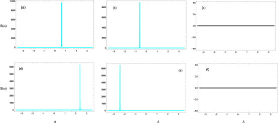
Figure 3: $\mathbb{S(\delta)}$ (in unit of $\Gamma^{-1}$) for (a)[(b)] $\varphi_{2}\left(\varphi_{3}\right)=\pi/2\left(3\pi/2\right)[3\pi/2\left(\pi/2\right)]$, $\left|\Omega_{o_{2},o_{1}}\right|=0.5\Gamma$ and $\left|\Omega_{m_{2},m_{1}}\right|=\Gamma.$ (d)[(e)] $\varphi_{2}\left(\varphi_{3}\right)=3\pi/2\left(\pi/2\right)[\pi/2\left(3\pi/2\right)]$, $\left|\Omega_{m_{2},m_{1},o_{2}}\right|=\Gamma,$ and $\left|\Omega_{o_{1}}\right|=0.1\Gamma[$ (c)[(f)] for examples, $\varphi_{2}\left(\varphi_{3}\right)=\pi\left(0\right)$ and $\left|\Omega_{m_{2},m_{1}o_{2},o_{1}}\right|=1\Gamma\ [\left|\Omega_{m_{2},m_{1}}\right|=1\Gamma,\left|\Omega_{o_{2}o_{1}}\right|=2\Gamma].$

Remarkably, with some appropriate relative strengths, the central two peaks of the three decaying bare-state suppress extremely while enhancing the sides one accordingly. However, when $\varphi_{2}\left(\varphi_{3}\right)\longrightarrow\pi(0)$ the trapping condition is satisfied, the two enhanced spectral lines of the central bare-state is cancelled [see Fig. 2[B](b)] reducing the area under the curve by $34\%$. However, no trapping state is there when $\varphi_{2}\left(\varphi_{3}\right)\longrightarrow\pi(0)$ [see Fig. 2[B](c)] except narrowing the spectral spectral lines. Moreover, there is a variety of very narrow single-peaked spectra for at least three different locations even with the one satisfying the trapping condition [see Fig. 2[C](b)] and compare its area under the curve with Fig. 2[C](a)]. This allows effective storage and manipulation of our one-atom quantum system like the two-atom quantum system of Ref. 2-atom but with the advantage of $47\%$ population trapping in the upper excited bare-state. Of course, this FGC-based result is novel and remarkable as compared with earlier related results.

Intriguingly, extending to a system of simple probability loss [see Fig. 1(b)] which generally has four-peak spectral profile can be manipulated to extremely narrowed-one-peak spectral profile at different locations for different choices of phases and fields strength [see Fig. 3(a-f)]. However, under the trapping condition of this system, the only decaying dressed bare-energy-state can also be completely darkened due to FGC. This is a major result meaning $100\%$ population trapping, a novel state of a darken atom. The atom remains in the dark state until the trapping condition is held on.

In conclusion, the FGC based atomic scheme is presented for spontaneous emission cancellation in contrast to the traditional SGC. The phases and strengths of the driven fields collectively modify the spontaneous emission spectrum due to which one to twelve peaks of varying widths arise. Further, experimentally easy controllable trapping condition is explored for spontaneous emission cancellation. This cancellation is from the whole set of four dressed states associated with the central bare-energy-state of the three set of closely spaced hyperfine decaying bare states. Extending this concept to a system of a simple loss, based on real atomic system, the brightened atom can also be darkened under its trapping condition, an interesting and viably novel phenomenon. The control of phases of the driving fields Phase and the coupling of multiple fields with an atomic system Zanch are now laboratory realities. These may be helpful in demonstrating the mechanism of the physical phenomenon of FGC in a laboratory for the spontaneous emission cancellation.

References

(1) G. S. Agarwal, Quantum Optics (Springer-Verlag, Berlin,
1974).
(2) G. Alzetta et al., Nuovo Cimento Soc. Ital. Fis. 36B, 5
(1974); E. Arimondo, in Progress in Optics, edited by E. Wolf (Elsevier,
Amsterdam, 1996), Vol. XXXV, p. 257.
(3) P. L. Knight, J. Phys. B 12, 3297 (1979); D. A. Cardimona et al., J. Phys. B 15, 55 (1982);
D. Agassi, Phys. Rev. A 30, 2449 (1984).
(4) B. M. Garraway and P. L. Knight, Phys. Rev. A 54,2379 (1969).
(5) S.-Y. Zhu, H. Chen, and H. Huang, Phys. Rev. Lett. 79,
205 (1997); Lewenstein et al. Phys. Rev. A 38,
808 (1988); S. Bay, P. Lambropoulos, and K. Mlmer, Phys. Rev.
A 79, 2654 (1997); A. G. Kofman, G. Kurizki, and B.
Sherman, J. Mod. Opt. 41, 353 (1994).
(6) For examples see, O. Kocharovskaya and Ya. I. Khanian, JETP Lett. 48,630 (1988); O. Kocharovskaya and P. Mandel, Phys. Rev. A
42, 523 (1990).
(7) M. O. Scully, Phys. Rev. Lett. 55, 2802 (1975); W.
Schleich and M. O. Scully, Phys. Rev. A 37, 1261(1987);
J. Bergou, M. Orszag, and M. O. Scully, Phys. Rev. A 38, 754 (1988).
(8) E. Paspalakis and P. L. Knight, Phys. Rev. Lett.
81, 293 (1998).
(9) S.-Y. Zhu and M. O. Scully, Phys. Rev. Lett. 76, 388 (1996).
(10) E. M. Macove and C. H. Keitel, Phys. Rev. Lett. 91,
123601 (2003).
(11) No trapping state exists in ”F. Ghafoor et al. Phys. Rev. A 62, 13811 (2000)”. In Ref.
”J. H. Wu et al., Phys. Rev. A 74, 033816 (2006)” Fano
type profile exists and the spectrum is like the Autler-Townes
triplet GhafoorF and obviously there is no CPT.
(12) Lee et al. Phys. Rev. A 55, 4454 (1997).
(13) Hakuta et al. Phys. Rev. Lett.
66, 596 (1991).
(14) H.-R. Xia, C.-Y. Ye, and S.-Y. Zhu, Phys. Rev. Lett. 77, 1032 (1996).
(15) Li Li, X. Wang, J. Yang, G. Lazarov, J. Qi, A. M. Lyyra, Phys.
Rev. Lett. 84, 4016 (2000).
(16) F. Ghafoor, Phys. Rev. A 84, 063849 (2011).
(17) G. Herzberg, Molecular Spectra and Molecular
Structure I; Spectra of Diatomic Molecules (Van Nostrand, Princeton, 1950)
(18) See for example, Z. G. Wang and H. R. Xia, Molecular
and Laser spectroscopy (Springer-Verlag, Berlin, 1991).
(19) F. Ghafoor, Phy. Rev. A (revision); For Autler-Townes
triplet spectrum see, F. Ghafoor, Opt. Commun. 284,1913 (2011); F.
Ghafoor, S. Qamar, S.- Y. Zhu, and M. S. Zubairy, Opt. Commun. 273,
464 (2007).
(20) For example, see Zuo et al. Phys. Rev. Lett. 97, 193904 (2004).
(21) M. O. Scully and M. S. Zubairy, Quantum Optics (Cambridge University Press, Cambridge, 1997).
(22) H. Autler and C. H. Townes, Phys. Rev. A 100, 703
(1955); P. L. Knight and P. W. Milonni, Phys. Rep. 66, 23 (1980).
(23) E. Paspalakis, C. H. Keitel, and P. L. Kinght, Phys. Rev. A,
58, 4868 (1998).
(24) L. Zhu et al., Science 270, 77 (1995); C. Chen and D. S.
Elliott, Phys. Rev. Lett. 65, 1737 (1990).