THE CORRELATION BETWEEN DISPERSION MEASURE AND X-RAY COLUMN DENSITY FROM RADIO PULSARS

Abstract

Pulsars are remarkable objects that emit across the entire electromagnetic spectrum, providing a powerful probe of the interstellar medium. In this study, we investigate the relation between dispersion measure (DM) and X-ray absorption column density $N_{\mathrm{H}}$ using 68 radio pulsars detected at X-ray energies with the Chandra X-ray Observatory or XMM-Newton. We find a best-fit empirical linear relation of $N_{\mathrm{H}}\rm\;(10^{20}\,cm^{-2})=0.30^{+0.13}_{-0.09}\;DM\;(pc\,cm^{-3})$, which corresponds to an average ionization of $10^{+4}_{-3}$%, confirming the ratio of one free electron per ten neutral hydrogen atoms commonly assumed in the literature. We also compare different $N_{\mathrm{H}}$ estimates and note that some $N_{\mathrm{H}}$ values obtained from X-ray observations are higher than the total Galactic Hi column density along the same line of sight, while the optical extinction generally gives the best $N_{\mathrm{H}}$ predictions.

1 INTRODUCTION

The broadband emission of pulsars from radio frequencies to $\gamma$-rays can be used to probe the physical conditions of the interstellar medium (ISM). Specifically, their radio pulsations allow accurate measurements of the free electron column density and their X-ray extinction traces the interstellar gas along the line of sight. Radio waves travelling in the ISM are dispersed by free electrons such that signals at lower frequencies propagate at a lower speed and hence arrive on Earth later than those at higher frequencies. The time delay ($\Delta t$) between two observing frequencies ($\nu_{1}$, $\nu_{2}$) depends on the dispersion measure (DM), which is the integrated free electron number density $n_{e}$ from Earth to the source at distance $d$:

$$\mathrm{DM}=\int_{0}^{d}{n_{e}\,\mathrm{d}l}=\frac{2\pi m_{e}c}{e^{2}}\left(\frac{1}{\nu_{1}^{2}}-\frac{1}{\nu_{2}^{2}}\right)^{-1}\Delta t\ ,$$ (1)

where $m_{e}$ and $e$ are electron mass and charge, respectively, and $c$ is the speed of light. Most free electrons in our Galaxy are found in the hot phase of the ISM, including Hii regions ionized by UV radiation from hot O or B type stars and the shock-heated interior of supernova remnants (SNRs). These sources can contribute significant DM up to a few hundred parsecs per cubic centimeter. At X-ray energies, photons are absorbed mostly by heavy elements in the interstellar gas due to the photoelectric effect. This has a strong energy dependence and is most prominent in the soft X-ray band. As a result, it modifies the observed low-energy portion of the X-ray spectrum and has to be accounted for in spectral modeling. The amount of extinction, which is expressed in terms of the equivalent atomic hydrogen column density $N_{\mathrm{H}}$, is sensitive to gas and molecular clouds, which traces the warm and cold phases of the ISM (see Wilms et al., 2000).

One natural question to ask is whether there is any correlation between DM and $N_{\mathrm{H}}$ in our Galaxy. Such a correlation can reflect the physical connection between different phases of the ISM. Also, it can provide a useful tool to estimate one quantity from the other, help plan new observations and determine X-ray luminosity upper limits in cases of non-detection. In the literature, an average ionization fraction of 10% in the ISM, i.e. one free electron per 10 equivalent hydrogen atoms, has been commonly assumed in order to infer $N_{\mathrm{H}}$ from DM (e.g., Seward & Wang, 1988; Kargaltsev et al., 2007; Gil et al., 2008; Camilo et al., 2012), but the justification for this choice has been unclear. X-ray-emitting radio pulsars offer a powerful diagnostic tool for a quantitative study of the correlation. Because they are model-independent and relatively straightforward to measure from radio timing, DM values are well determined, typically to better than a fractional uncertainty of $10^{-3}$. However, what has made the determination of any DM-$N_{\mathrm{H}}$ correlation difficult in the past is the lack of high-quality X-ray data for $N_{\mathrm{H}}$ measurements. In particular, previous generations of X-ray telescopes had poor angular resolution that precluded discerning the pulsar emission from that of the surrounding SNRs and pulsar wind nebulae (PWNe). Thanks to new X-ray missions such as the Chandra X-ray Observatory and XMM-Newton, precise measurements of $N_{\mathrm{H}}$ have been obtained for many pulsars in recent years, allowing a statistical study of $N_{\mathrm{H}}$ values for the first time.

In this paper, we compile a list of DM and $N_{\mathrm{H}}$ values for 68 X-ray-emitting radio pulsars using the latest Chandra and XMM-Newton measurements reported in the literature. We found a clear correlation between these two column densities and obtained a best-fit empirical relation of $10^{+4}_{-3}$% ionization. In Section 2, we describe our sample selection criteria. The statistical analysis and results are presented in Section 3, and we discuss the implications of our results in Section 4.

2 SAMPLE SELECTION

We started with a list of X-ray detected radio pulsars from Possenti et al. (2002), Becker & Aschenbach (2002), Pavlov et al. (2007), Kargaltsev & Pavlov (2008), and Kargaltsev & Pavlov (2010), then expanded the sample through careful literature searches for updated observational results and recent discoveries. The latter include three magnetars that show radio emission (Camilo et al., 2006, 2007; Levin et al., 2010) and over a dozen new pulsars identified in $\gamma$-rays with the Fermi Gamma-ray Space Telescope and subsequently detected in follow-up radio and X-ray observations (see Marelli et al., 2011). Finally to complete the list, we went through the Chandra and XMM-Newton data archive to search for pulsar observations, and looked up relevant publications based on these data.

The pulsar DMs are adopted from the ATNF Pulsar Catalog (Manchester et al., 2005). They are all very well measured with negligible uncertainties compared to those for $N_{\mathrm{H}}$. On the other hand, it is much more difficult to determine $N_{\mathrm{H}}$, because this requires a strong X-ray source and good knowledge of the intrinsic emission spectrum. The X-ray emission of pulsars is not fully understood; commonly used models include a blackbody (BB) and a neutron-star hydrogen atmosphere (NSA) for the thermal emission, and a power law (PL) for the non-thermal emission. More complicated models consisting of thermal and non-thermal components are sometimes used. To minimize any bias, we selected the $N_{\mathrm{H}}$ values for our sample according to the following criteria:

1. We restricted our choices to those in the latest studies using the Chandra and XMM-Newton observations, since the good angular resolution and sensitivity of these telescopes offer high-quality spectra with minimal background contamination. Any joint fits with other X-ray telescopes are not considered, in order to avoid cross-calibration uncertainties.

2. We adopted only $N_{\mathrm{H}}$ values from actual X-ray spectral fits in which the $N_{\mathrm{H}}$ is allowed to vary freely, and ignored any $N_{\mathrm{H}}$ inferred from DM, optical extinction (A_V), or total Galactic Hi column density.

3. $N_{\mathrm{H}}$ from the best-fit spectral model is always preferred, unless there are physical arguments favoring another model. If different emission models give the same goodness-of-fit and the authors do not indicate a clear preference, we choose the simpler one. For example, we prefer a BB model over an NSA model, since the latter requires more assumptions, including the atmosphere composition, surface magnetic field and gravity.

4. For pulsars associated with bright PWNe, the nebular $N_{\mathrm{H}}$ values are adopted if they are better constrained than those of the pulsars, because the simple PL spectra of PWNe can reduce systematic uncertainties in spectral modeling. $N_{\mathrm{H}}$ from SNRs are used in a few cases when the pulsars and PWNe are too faint for useful $N_{\mathrm{H}}$ measurements.

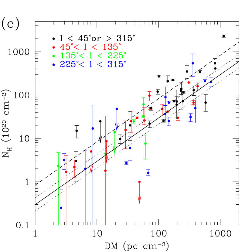
Figure 1: $N_{\mathrm{H}}$ versus DM for 68 pulsars. (a) Data points in gray color, including the Vela pulsar, PSR B0540$-$69, and $N_{\mathrm{H}}$ measurements with fractional uncertainties larger than 80% or only upper limits are not used in the fit. The red solid and dotted lines show the best linear fit with the 90% confidence interval, and the blue dashed line is the same fit ignoring measurement uncertainties. These correspond to $10^{+4}_{-3}$% and 4% ionization, respectively. Uncertainties in DM are negligible. The same plot is shown in (b) and (c) with different color schemes, indicating the pulsar vertical distance from the Galactic Plane and their Galactic longitudes, respectively.

Our final sample contains 68 pulsars. One of them (PSR B0540$-$69) is extragalactic and only two (PSRs J1740$-$5340 and B1821$-$24) are in globular clusters; cluster pulsars are generally too faint for precise $N_{\mathrm{H}}$ measurements. The pulsar DM and $N_{\mathrm{H}}$ values are listed in Table THE CORRELATION BETWEEN DISPERSION MEASURE AND X-RAY COLUMN DENSITY FROM RADIO PULSARS and plotted in Figure 1. The reported statistical uncertainties and upper limits for $N_{\mathrm{H}}$ are at 90% confidence level, i.e. 1.6$\sigma$. We list in the Table the X-ray spectral models used to obtain $N_{\mathrm{H}}$. The choice of spectral model is clear in all cases except PSRs J1622$-$4950 and B1757$-$24, for which both thermal and non-thermal fits are acceptable. Nonetheless, $N_{\mathrm{H}}$ from different fits only varies by a factor of 2 for J1622$-$4950 and does not change for B1757$-$24. Therefore, we conclude that systematic bias induced by spectral models is minimal.

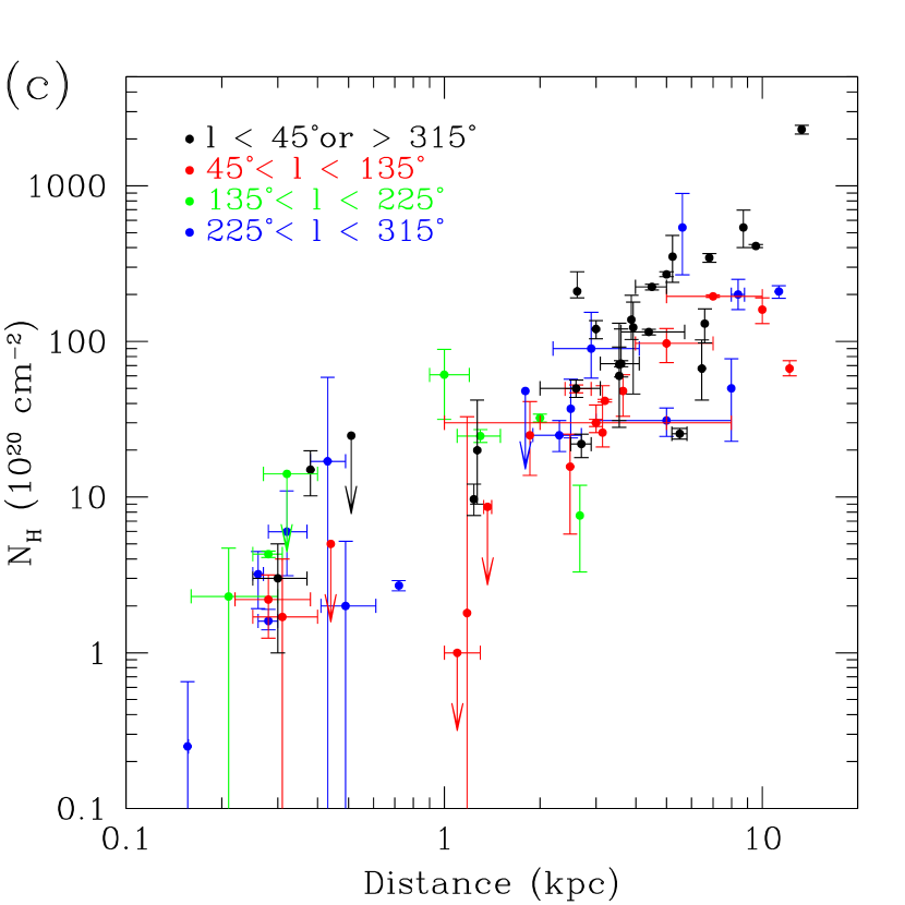
Figure 2: $N_{\mathrm{H}}$ versus distance for Galactic pulsars. PSR B0540$-$69 is not shown here. (a) The colors indicate different types of distance measurement. We did not estimate the uncertainties for the DM distances. The same plot with different color schemes is shown in (b) and (c), indicating the pulsar vertical distance from the Galactic Plane and their Galactic longitudes, respectively.

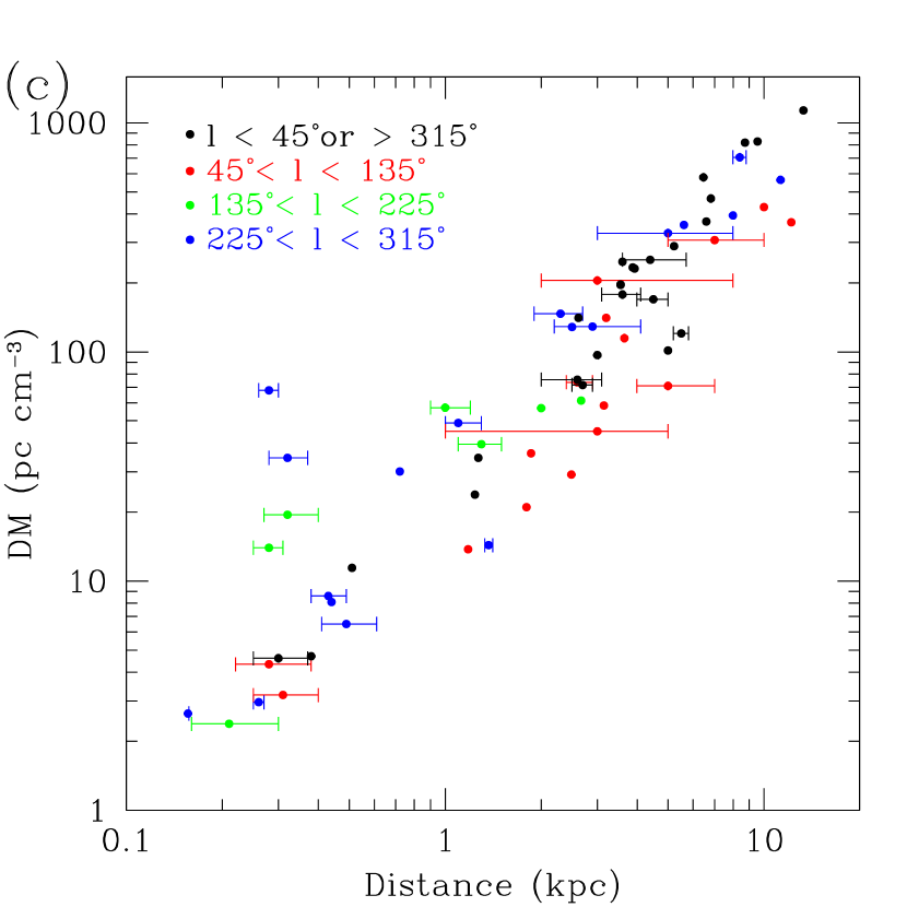
Figure 3: Same as Figure 2, but for DM versus distance. Uncertainties in DM are not plotted, as they are smaller than the data points.

Table THE CORRELATION BETWEEN DISPERSION MEASURE AND X-RAY COLUMN DENSITY FROM RADIO PULSARS also shows the pulsar Galactic coordinates ($l$, $b$) and distances, and this information was used to calculate the vertical height ($z$) from the Galactic Plane. The coordinates are taken from the ATNF Pulsar Catalog and distance estimates are obtained from parallax measurements, Hi absorption measurements of the pulsars or the associated SNRs, or DM using the NE2001 Galactic electron density model (Cordes & Lazio, 2002). If available, parallax distances are always preferred since they are the most accurate. All parallax and Hi distances are adopted from Verbiest et al. (2012) and references therein, and have been corrected for the Lutz-Kelker bias, except for PSR J1023+0038, which has a recent parallax measurement by Deller et al. (2012). For DM distances, we did not attempt to derive the uncertainties, but note that the fractional uncertainties could be 25% or larger (see e.g., Camilo et al., 2009). Finally, there are exceptional cases in which previous studies argue for different distances than the DM-estimated ones. They are noted in the Table. The pulsar $N_{\mathrm{H}}$ and DM are plotted against distance in Figures 2 and 3, respectively.

3 ANALYSIS & RESULTS

Figure 1 shows a positive correlation between the pulsar DM and $N_{\mathrm{H}}$ values, with deviations ranging from a factor of a few to an order of magnitude. There are some obvious outliers, including the Vela pulsar (PSR B0833$-$45), the double pulsar (PSR J0737$-$3039), and PSR J1747$-$2809 in the Galactic Center direction. To quantify the DM-$N_{\mathrm{H}}$ correlation, we ignored pulsars with $N_{\mathrm{H}}$ upper limits and obtained a Pearson’s correlation coefficient of 0.72. This is significant since the one-tailed probability of such a correlation arising by chance from unrelated variables is only $4\times 10^{-5}$. More useful is an empirical relation between these two observables. We performed a linear fit to the data by minimizing the $\chi^{2}$ value. $N_{\mathrm{H}}$ measurements with fractional uncertainties larger than 80% or upper limits only (gray points in Figure 1) are excluded in the fit. We also ignored the Vela pulsar, which is located in the Gum Nebula inside the hot and low-density Local Bubble, and PSR B0540$-$69, which is in the Large Magellanic Cloud (LMC), because they seem unlikely to follow the DM-$N_{\mathrm{H}}$ correlation as would other Galactic sources. Only statistical uncertainties in $N_{\mathrm{H}}$ are considered in the $\chi^{2}$-fit since uncertainties in DM are negligible. Also, we did not attempt to model the systematic uncertainties, but we note that the ones introduced by different photoelectric absorption models and elemental abundances, or by cross-calibration between telescopes are only at a few percent level (see Wilms et al., 2000; Tsujimoto et al., 2011), relatively small compared to the statistical uncertainties. Assuming $N_{\mathrm{H}}$ and DM are directly proportional, the best fit gives

$$N_{\mathrm{H}}\rm\;(10^{20}\,cm^{-2})=0.30^{+0.13}_{-0.09}\;DM\;(pc\,cm^{-3})\ ,$$ (2)

corresponding to an average ionization of $10^{+4}_{-3}$%. The 90% confidence interval is quoted here, which is obtained from 10000 simulations via bootstrapping resampling (Efron & Tibshirani, 1993). The result is plotted in Figure 1. We also tried fitting a more general linear relation by fitting the y-intercept as well, but found that the latter is consistent with zero at 90% confidence. If we ignore the measurement uncertainties in $N_{\mathrm{H}}$ and perform a least squares fit, we obtain $N_{\mathrm{H}}\rm\;(10^{20}\,cm^{-2})=0.83\;DM\;(pc\,cm^{-3})$, giving a lower average ionization of 4%.

To check if the DM-$N_{\mathrm{H}}$ relation could depend on the source location in the Galaxy, we divided the sample into groups according to their vertical height from the plane and their Galactic longitudes. The results are shown in Figures 1(b) and 1(c), respectively. In the high-DM regime, sources toward the Galactic Center direction, e.g., PSRs J1747$-$2958 and J1747$-$2809, show a hint of a larger $N_{\mathrm{H}}$-to-DM ratio. However, the systematic variation is less clear at lower DM and our limited sample precludes a detailed analysis. In Figure 2 we plotted $N_{\mathrm{H}}$ against distance. This indicates a general correlation, albeit with a large scatter. There is also a hint that for sources at a similar distance, $N_{\mathrm{H}}$ is systematically larger near the Galactic Plane (Figure 2(b)), however, the dependency on Galactic longitude is less clear (Figure 2(c)). The DM variation with distance is presented in Figure 3. While this may seem to exhibit a good correlation at large distances, we note that sources with DM-derived distances provide no new information, only the NE2001 model prediction. In addition, there is a very large range of DMs for nearby pulsars around 300 pc, from $2.4\pm 0.2$ pc cm^-3 for PSR J0108$-$1431 to $68\pm 1.6$ pc cm^-3 for the Vela pulsar, spanning nearly a factor of 30. Similar to $N_{\mathrm{H}}$, Figure 3(b) also indicates a higher DM toward the Galactic Plane.

4 DISCUSSION

We have investigated the DM-$N_{\mathrm{H}}$ connection for 68 radio pulsars detected with Chandra or XMM-Newton. We found a good correlation between these two column densities, suggesting that free electrons in the Galaxy generally trace the interstellar gas. That said, some $N_{\mathrm{H}}$ values in Figure 1 show significant deviation from the best-fit line, by a factor of a few up to an order of magnitude. This could be attributed to inhomogeneity of the ISM, possibly due to molecular clouds, supernova remnants, or Hii regions in the line of sight. Such an effect is more prominent for nearby sources, since the distribution of free electrons and interstellar gas is highly anisotropic around the Local Bubble (see Taylor & Cordes, 1993; Lallement et al., 2003). In particular, there is significant DM contribution from the Gum Nebula (Taylor & Cordes, 1993), resulting in a wide range of DMs for pulsars within $\sim$300 pc (e.g., the Vela pulsar and PSR J0737$-$3039; see Figure 3). At large distances, local fluctuations are expected to average out and the scatter of $N_{\mathrm{H}}$ and DM with respect to distance likely arises from Galactic structure, such as the disk, spiral arms, and different scale heights of various ISM components (see Cox, 2005). We have attempted to identify any systematic trends in DM and $N_{\mathrm{H}}$ with respect to source location. While Figures 2(b) and 3(b) hint at higher $N_{\mathrm{H}}$ and DM toward the Galactic Plane, more sources are needed for a quantitative comparison with the detailed Galactic structure. Beyond our Galaxy, we note that while PSR B0540$-$69 in the LMC was not used in the fit, its DM-to-$N_{\mathrm{H}}$ ratio lies close to the best-fit line in Figure 1. This is somewhat surprising because of the different interstellar abundances in the LMC than in our Galaxy (Russell & Dopita, 1992). We argue that this could merely be a coincidence rather than the general case. Indeed, the LMC contributes 90% of the $N_{\mathrm{H}}$ toward PSR B0540$-$69 (Park et al., 2010) but only two thirds of the DM (Manchester et al., 2006).

The DM-$N_{\mathrm{H}}$ correlation can be used to estimate one quantity from the other, offering a useful tool for pulsar observations. For instance, radio pulsations have been claimed from the magnetar 4U 0142+61 with a DM of $27\pm 5$ pc cm^-3 (Malofeev et al., 2010). Given its $N_{\mathrm{H}}$ value of $9.6\pm 0.2\times 10^{21}$ cm^-2 (Göhler et al., 2005), the claimed DM seems somewhat small when compared to other sources of similar $N_{\mathrm{H}}$ in Figure 1. For X-ray observations, there are many cases requiring a priori knowledge of $N_{\mathrm{H}}$, including flux estimates when planning for new observations, measuring the intrinsic spectra of faint sources, and deriving luminosity limits for non-detection. In many previous studies, $N_{\mathrm{H}}$ is inferred from the DM by assuming one free electron per ten neutral hydrogen atoms (e.g. Kargaltsev et al., 2007; Camilo et al., 2012). Our result directly confirms that this is a reasonable approximation, but as a caveat, the scatter in $N_{\mathrm{H}}$ is typically a factor of a few up to an order of magnitude.

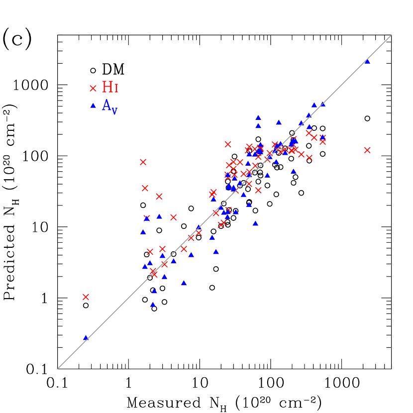
Figure 4: Comparison between $N_{\mathrm{H}}$ estimates and measurements. The underlying plots in (a) and (b) are the same as Figures 1 and 2, respectively. The red crosses indicate the total line-of-sight Galactic Hi column densities for each pulsar, given by 21 cm radio observations (Kalberla et al., 2005). The blue triangles show estimates based on A_V (see text). In (c), the open circles represent predictions from our best-fit DM-$N_{\mathrm{H}}$ relation.

In addition to DM, the total Galactic Hi column density from 21-cm radio surveys (e.g., Kalberla et al., 2005) and A_V have also been used as proxies for the X-ray absorption (e.g., Olausen et al., 2013). These $N_{\mathrm{H}}$ estimates are plotted in Figure 4. It is clear that some X-ray-inferred $N_{\mathrm{H}}$ values exceed the total Hi column density of the Galaxy. As shown in the Figure, the latter saturates at $\sim 10^{22}$ cm^-2, resulting in gross underestimates for high-DM ($\gtrsim 100$ pc cm^-3) or distant ($\gtrsim 3$ kpc) pulsars. It has been reported that at high Galactic column densities $\gtrsim 10^{21}$ cm^-2, which occur at low Galactic latitudes, the X-ray absorption columns are generally larger than the Hi columns by a factor of 1.5–3 (Arabadjis & Bregman, 1999; Baumgartner & Mushotzky, 2006). This agrees with our result and indicates significant X-ray absorption due to molecular clouds rather than neutral hydrogen atoms, hence, the Hi column may not be a good tracer for the X-ray absorption.

A_V, on the other hand, is caused by grains of the same heavy elements that give rise to X-ray absorption, therefore, it highly correlates with $N_{\mathrm{H}}$ (e.g., Predehl & Schmitt, 1995; Güver & Özel, 2009). Given a pulsar’s position and distance, A_V can be estimated from the 3D extinction maps of the Galaxy (e.g., Drimmel et al., 2003), and then $N_{\mathrm{H}}$ can be deduced from the empirical relation $N_{\mathrm{H}}$( cm^-2)=$2.21\times 10^{21}$ A_V (mag) (Güver & Özel, 2009). As shown in Figure 4, this method seems to give the best agreement between measured and predicted values, especially for the highest-$N_{\mathrm{H}}$ pulsars. It is worth noting that in some cases DMs were used to infer the pulsar distances, which then give A_V and $N_{\mathrm{H}}$. This generally provides better results than directly employing the DM-$N_{\mathrm{H}}$ correlation. We believe that this is because the A_V map reflects the distribution of heavy elements in the Galaxy, whereas this crucial information cannot be obtained from DM.

5 CONCLUSION AND OUTLOOK

We have compiled a list of 68 pulsar $N_{\mathrm{H}}$ measurements reported in the literature using Chandra and XMM-Newton observations, and compared the $N_{\mathrm{H}}$ values with the DMs and distances. Our results show a good correlation between DM and $N_{\mathrm{H}}$, with a correlation coefficient of 0.72. We obtained an empirical linear relation $N_{\mathrm{H}}\rm\;(10^{20}\,cm^{-2})=0.30^{+0.13}_{-0.09}\;DM\;(pc\,cm^{-3})$, implying an average ionization of $10^{+4}_{-3}$%. This confirms the ratio of one free electron to ten neutral hydrogen atoms commonly used in previous studies. Our finding provides a useful tool to estimate $N_{\mathrm{H}}$ from DM. We compare to other $N_{\mathrm{H}}$ estimates based on the neutral hydrogen column density and A_V, and find that the latter gives the best results, while Hi and our empirical DM-$N_{\mathrm{H}}$ relation tend to give underestimates in the high-$N_{\mathrm{H}}$ regime.

The next generation of X-ray missions, including eROSITA (Predehl et al., 2010) and the proposed Neutron Star Interior Composition Explorer (NICER; Gendreau et al., 2012), will significantly expand the pulsar $N_{\mathrm{H}}$ sample. In addition, the foreseen Square Kilometer Array (SKA) can provide parallax measurements of a few thousand radio pulsars (Smits et al., 2011). Together these will allow a detailed study of the DM-$N_{\mathrm{H}}$ relation in different parts of the Galaxy and its connection with the Galactic structure. In addition to pulsars, it should be possible to compile a database of $N_{\mathrm{H}}$ measurements for other Galactic X-ray sources, such as stars, supernova remnants, cataclysmic variables, stellar clusters, white dwarfs, and X-ray binaries, and compare with their distances to build a 3D $N_{\mathrm{H}}$ map of our Galaxy.

Table 1: DM, $N_{\mathrm{H}}$, and Distances for the 68 Pulsars Used in This Study

PSR	DM	$N_{\mathrm{H}}$	Distance	$l$	$b$	$z$	Model	Ref.
	(pc cm-3)	($10^{20}$ cm-2)	(kpc)	(deg)	(deg)	(pc)
J0030+0451	4.333$\pm$0.001	2.2$\pm$1.0	$0.28^{+0.10}_{-0.06}$p	113.1	$-57.6$	$-236$	NSA$\times$3	1
J0108$-$1431	$2.4\pm 0.2$	$2\pm 2$	$0.21^{+0.09}_{-0.05}$p	140.9	$-76.8$	$-205$	BB	2
B0136+57	73.779$\pm$0.006	$50\pm 3$	$2.6^{+0.3}_{-0.2}$p	129.2	$-4.0$	$-183$	PL	3
J0205+6449	140.7$\pm$0.3	41.6${}^{+0.8}_{-0.7}$	3.2o	130.7	+3.1	+172	PL+RS (SNR)	4, 5
J0218+4232	61.252$\pm$0.005	$8\pm 4$	$2.67$d	139.5	$-17.5$	$-804$	PL	6
B0355+54	57.1420$\pm$0.0003	$60\pm 30$	$1.0^{+0.2}_{-0.1}$p	148.2	+0.8	+14	PL (PWN)	7
J0437$-$4715	2.64476$\pm$0.00007	$0.25^{+0.40}_{-0.24}$	$0.156\pm 0.001$p	253.4	$-42.0$	$-104$	PL+NSA$\times$2	8
B0531+21 (Crab)	56.791$\pm$0.001	32$\pm$2	2.00o	184.6	$-5.8$	$-202$	PL	9, 10
J0538+2817	39.570$\pm$0.001	$25\pm 2$	$1.3\pm{0.2}$p	179.7	$-1.7$	$-38$	BB	11
B0540$-$69	$146.6\pm 0.2$	$67\pm 5$	50o	279.7	$-31.5$	$-26137$	PL (SNR)	12, 13
B0628$-$28	34.468$\pm$0.017	$6^{+5}_{-3}$	$0.32^{+0.05}_{-0.04}$p	237.0	$-$16.8	$-$92.3	PL	14
B0656+14	13.977$\pm$0.013	4.3$\pm$0.2	$0.28\pm 0.03$p	201.1	+8.3	+40	PL+BB$\times$2	15
J0737$-$3039	48.920$\pm$0.005	$<1$	$1.1^{+0.2}_{-0.1}$p	245.2	$-$4.5	$-$86	BB$\times$2	16
B0823+26	19.454$\pm$0.004	$<14$	$0.32^{+0.08}_{-0.05}$p	197.0	+31.7	+168	PL	17
B0833$-$45 (Vela)	67.99$\pm$0.01	$1.6^{+0.3}_{-0.2}$	$0.28\pm 0.02$p	263.6	$-2.8$	$-14$	PL (PWN)	18
B0950+08	2.958$\pm$0.003	3.2$\pm$1.3	0.261$\pm$0.005p	228.9	+43.7	+180	PL+BB	19
J1016$-$5857	394.2$\pm$0.2	50$\pm$30	8.00d	284.1	$-1.9$	$-263$	PL	20
J1023+0038	14.325$\pm$0.010	$<9$	1.37$\pm$0.04p	243.5	+45.8	+980	PL+NSA	21
J1024$-$0719	6.48520$\pm$0.00008	$2^{+3}_{-2}$	$0.49^{+0.12}_{-0.08}$p	251.7	+40.5	+318	BB	22
B1046$-$58	129.1$\pm$0.2	90${}^{+60}_{-30}$	$2.9^{+1.2}_{-0.7}$h	287.4	+0.6	+29	PL	23
B1055$-$52	30.1$\pm$0.5	$2.7\pm 0.2$	0.72d	286.0	+6.7	+84	PL+BB$\times$2	15
J1119$-$6127	707.4$\pm$1.3	$200^{+50}_{-40}$	8.4$\pm$0.4o	292.2	$-0.5$	$-78.7$	PL+BB	24, 25
J1124$-$5916	330$\pm$2	31$\pm$6	5${}^{+3}_{-2}$h	292.0	+1.8	+153	PL	26
J1231$-$1411	8.090$\pm$0.001	$<5$	0.44d	295.5	+48.4	+329	NSA+PL	27
B1259$-$63	146.72$\pm$0.03	$25^{+6}_{-5}$	2.3$\pm$0.4o	304.2	$-$1.0	$-$40	PL	28, 29
J1357$-$6429	128.5$\pm$0.7	37${}^{+20}_{-13}$	2.50d	309.9	$-$2.5	$-$110	PL (PWN)	30
J1400$-$6325	563$\pm$4	$209\pm 20$	11.27d	310.6	$-$1.6	$-$313	PL (PWN)	31
J1420$-$6048	358.8$\pm$0.2	$540^{+350}_{-270}$	5.61d	313.5	+0.2	+22	PL (PWN)	32
B1451$-$68	8.6$\pm$0.2	17${}^{+40}_{-17}$	$0.43^{+0.06}_{-0.05}$p	313.9	$-$8.5	$-64$	PL+BB	33
J1509$-$5850	140.6$\pm$0.8	210${}^{+70}_{-20}$	2.62d	320.0	$-$0.6	$-$28	PL (PWN)	34
B1509$-$58	252.5$\pm$0.3	115$\pm 5$	4.4${}^{+1.3}_{-0.8}$h	320.3	$-$1.2	$-$89	PL (PWN)	35
J1550$-$5418	830$\pm$50	410$\pm$10	9.55d	327.2	$-$0.1	$-$22	PL+BB	36
J1614$-$2230	34.4865$\pm$0.0001	20${}^{+22}_{-11}$	1.27d	352.6	+20.2	+438	BB$\times$2	37
J1617$-$5055	467$\pm$5	345$\pm 20$	6.82d	332.5	$-$0.3	$-$33	PL	38
J1622$-$4950	820$\pm$30	540${}^{+160}_{-140}$	8.73d	333.8	$-$0.1	$-$16	BB	39
B1706$-$44	75.69$\pm$0.05	50$\pm 6$	2.6${}^{+0.5}_{-0.6}$h	343.1	$-$2.7	$-$122	PL (PWN)	40
J1718$-$3718	371.1$\pm$1.7	130$\pm 30$	6.6d	349.8	+0.2	+25	BB	41
J1718$-$3825	247.4$\pm$0.3	72${}^{+50}_{-13}$	3.6d	349.0	$-$0.4	$-$27	PL (PWN)	42
J1734$-$3333	578$\pm$9	$70^{+40}_{-30}$	6.46d	354.8	$-$0.4	$-$49	BB	43
J1740$-$5340	71.8$\pm$0.2	$22\pm 4$	2.7$\pm$0.2o	338.2	$-$12.0	$-$560	PL	44, 45
J1740+1000	23.85$\pm$0.05	$10\pm 2$	1.24d	34.0	+20.3	+430	PL+BB	46
J1741$-$2054	4.7$\pm$0.1	15$\pm 5$	0.38d	6.4	+4.9	+33	PL (PWN)	47
J1747$-$2809	1133$\pm$3	2300$\pm$150	13.31d	0.9	+0.1	+18	PL (PWN)	48
J1747$-$2958	101.5$\pm$1.6	270$\pm$10	5o	359.3	$-$0.8	$-$73	PL (PWN)	49, 50
B1757$-$24	289$\pm$10	350${}^{+130}_{-110}$	5.22d	5.3	$-$0.9	$-$80	PL	51
B1800$-$21	233.99$\pm$0.05	138${}^{+60}_{-35}$	3.88d	8.4	+0.2	+10	PL (PWN)	52
J1809$-$1917	197.1$\pm$0.4	71${}^{+60}_{-40}$	3.55d	11.1	+0.1	+5	PL	53
J1809$-$1943	178$\pm$5	72$\pm 3$	$3.6\pm 0.5$h	10.7	$-$0.2	$-$10	BB$\times$3	54
J1819$-$1458	196.0$\pm$0.4	60$\pm 30$	3.55d	16.0	+0.1	+5	BB	55
B1821$-$24	120.502$\pm$0.002	$26\pm 2$	5.5$\pm$0.3o	7.8	$-$5.6	$-$535	PL	56, 57
B1823$-$13	231$\pm$1	$120^{+60}_{-80}$	3.93d	18.0	$-$0.7	$-$47	PL (PWN)	58
J1833$-$1034	169.5$\pm$0.1	$224^{+9}_{-10}$	$4.5\pm 0.5^{\rm h}$	21.5	$-$0.9	$-$70	PL	59
B1853+01	96.74$\pm$0.12	120$\pm 16$	$3^{\rm o}$	34.6	$-0.5$	$-26$	VNEI$\times$2 (SNR)	60, 61
J1930+1852	308$\pm$4	195$\pm$4	$7^{+3}_{-2}$h	54.1	+0.3	+32	PL (PWN)	62
B1929+10	3.180$\pm$0.004	$1.7^{+2.3}_{-1.7}$	$0.31^{+0.09}_{-0.06}$p	47.4	$-3.9$	$-21$	PL+BB	63
B1937+21	71.0398$\pm$0.0002	$97\pm 24$	$5^{+2}_{-1}$p	57.5	$-0.3$	$-25$	PL	64
B1951+32	45.006$\pm$0.0190	$30\pm 2$	$3\pm 2^{\rm h}$	68.8	+2.8	+148	PL	65
B1957+20	29.1168$\pm$0.0007	$16\pm 10$	2.49d	59.2	$-4.7$	$-204$	PL	66
J2021+3651	368$\pm$1	67${}^{+8}_{-7}$	12.19d	75.2	+0.1	+24	PL	67
J2022+3842	429.1$\pm$0.5	160$\pm$30	10o	76.9	+1.0	+168	PL	68
J2032+4127	114.8$\pm$0.1	$48^{+13}_{-15}$	3.65d	80.2	+1.0	+66	PL	69
J2043+2740	21.0$\pm$0.1	$<50$	$1.8^{\rm d}$	70.6	$-9.2$	$-286$	BB	17
J2124$-$3358	4.601$\pm$0.003	3$\pm$2	$0.30^{+0.07}_{-0.05}$p	10.9	$-45.4$	$-214$	PL+BB	22
B2224+65	36.079$\pm$0.009	25${}^{+16}_{-11}$	1.86d	108.6	+6.8	+222	PL	70
J2229+6114	204.97$\pm$0.02	30${}^{+9}_{-4}$	$3^{+5}_{-1}$o	106.6	+2.9	+154	PL	71, 72
J2241$-$5236	11.41085$\pm$0.00003	$<25$	0.51d	337.5	$-$54.9	$-417$	PL	69
J2302+4442	13.762$\pm$0.006	$2^{+31}_{-2}$	1.18d	103.4	$-$14.0	$-286$	NSA	73
B2334+61	58.410$\pm$0.015	26${}^{+26}_{-5}$	3.15d	114.3	+0.2	+13	BB	74

.

Note. — Uncertainties and upper limits on $N_{\mathrm{H}}$ are all scaled to the 90% confidence level, i.e. $1.6\sigma$.

References. — (1) Bogdanov & Grindlay 2009; (2) Posselt et al. 2012a; (3) Maselli et al. 2011; (4) Gotthelf et al. 2007; (5) Roberts et al. 1993; (6) Webb et al. 2004; (7) Tepedelenliǧlu & Ögelman 2007; (8) Durant et al. 2012; (9) Weisskopf et al. 2011; (10) Trimble 1973; (11) Ng et al. 2007; (12) Park et al. 2010; (13) Freedman et al. 2001; (14) Becker et al. 2005; (15) De Luca et al. 2005; (16) Possenti et al. 2008; (17) Becker et al. 2004; (18) LaMassa et al. 2008; (19) Zavlin & Pavlov 2004; (20) Camilo et al. 2004; (21) Bogdanov et al. 2011a; (22) Zavlin 2006; (23) Gonzalez et al. 2006; (24) Ng et al. 2012; (25) Caswell et al. 2004; (26) Hughes et al. 2003; (27) Ransom et al. 2011; (28) Pavlov et al. 2011; (29) Negueruela et al. 2011; (30) Chang et al. 2012; (31) Renaud et al. 2010; (32) Ng et al. 2005; (33) Posselt et al. 2012b; (34) Kargaltsev et al. 2008; (35) Schöck et al. 2010; (36) Ng et al. 2011; (37) Pancrazi et al. 2012; (38) Kargaltsev et al. 2009; (39) Anderson et al. 2012; (40) Romani et al. 2005; (41) Zhu et al. 2011; (42) Hinton et al. 2007; (43) Olausen et al. 2013; (44) Bogdanov et al. 2010; (45) Reid & Gizis 1998; (46) Kargaltsev et al. 2012; (47) Romani et al. 2010 (48) Holler et al. 2012; (49) Gaensler et al. 2004; (50) Gaensler et al. 2004; (51) Kaspi et al. 2001; (52) Kargaltsev et al. 2007; (53) Kargaltsev & Pavlov 2007; (54) Bernardini et al. 2009; (55) Rea et al. 2009; (56) Bogdanov et al. 2011b; (57) Harris 1996; (58) Pavlov et al. 2008; (59) Matheson & Safi-Harb 2010; (60) Shelton et al. 2004; (61) Claussen et al. 1996; (62) Temim et al. 2010; (63) Misanovic et al. 2008; (64) Ng et al. 2013, in preparation; (65) Li et al. 2005; (66) Guillemot et al. 2012; (67) Van Etten et al. 2008; (68) Arzoumanian et al. 2011; (69) Marelli 2012; (70) Hui et al. 2012; (71) Marelli et al. 2011; (72) Halpern et al. 2001; (73) Cognard et al. 2011; (74) McGowan et al. 2006

References

- Anderson et al. (2012) Anderson, G. E., Gaensler, B. M., Slane, P. O., et al. 2012, ApJ, 751, 53
- Arabadjis & Bregman (1999) Arabadjis, J. S., & Bregman, J. N. 1999, ApJ, 510, 806
- Arzoumanian et al. (2011) Arzoumanian, Z., Gotthelf, E. V., Ransom, S. M., et al. 2011, ApJ, 739, 39
- Baumgartner & Mushotzky (2006) Baumgartner, W. H., & Mushotzky, R. F. 2006, ApJ, 639, 929
- Becker & Aschenbach (2002) Becker, W., & Aschenbach, B. 2002, in Neutron Stars, Pulsars, and Supernova Remnants, ed. W. Becker, H. Lesch, & J. Trümper, 64
- Becker et al. (2005) Becker, W., Jessner, A., Kramer, M., Testa, V., & Howaldt, C. 2005, ApJ, 633, 367
- Becker et al. (2004) Becker, W., Weisskopf, M. C., Tennant, A. F., et al. 2004, ApJ, 615, 908
- Bernardini et al. (2009) Bernardini, F., Israel, G. L., Dall’Osso, S., et al. 2009, A&A, 498, 195
- Bogdanov et al. (2011a) Bogdanov, S., Archibald, A. M., Hessels, J. W. T., et al. 2011a, ApJ, 742, 97
- Bogdanov & Grindlay (2009) Bogdanov, S., & Grindlay, J. E. 2009, ApJ, 703, 1557
- Bogdanov et al. (2010) Bogdanov, S., van den Berg, M., Heinke, C. O., et al. 2010, ApJ, 709, 241
- Bogdanov et al. (2011b) Bogdanov, S., van den Berg, M., Servillat, M., et al. 2011b, ApJ, 730, 81
- Camilo et al. (2004) Camilo, F., Gaensler, B. M., Gotthelf, E. V., Halpern, J. P., & Manchester, R. N. 2004, ApJ, 616, 1118
- Camilo et al. (2009) Camilo, F., Ng, C.-Y., Gaensler, B. M., et al. 2009, ApJ, 703, L55
- Camilo et al. (2012) Camilo, F., Ransom, S. M., Chatterjee, S., Johnston, S., & Demorest, P. 2012, ApJ, 746, 63
- Camilo et al. (2007) Camilo, F., Ransom, S. M., Halpern, J. P., & Reynolds, J. 2007, ApJ, 666, L93
- Camilo et al. (2006) Camilo, F., Ransom, S. M., Halpern, J. P., et al. 2006, Nature, 442, 892
- Caswell et al. (2004) Caswell, J. L., McClure-Griffiths, N. M., & Cheung, M. C. M. 2004, MNRAS, 352, 1405
- Chang et al. (2012) Chang, C., Pavlov, G. G., Kargaltsev, O., & Shibanov, Y. A. 2012, ApJ, 744, 81
- Claussen et al. (1996) Claussen, M. J., Wilking, B. A., Benson, P. J., et al. 1996, ApJS, 106, 111
- Cognard et al. (2011) Cognard, I., Guillemot, L., Johnson, T. J., et al. 2011, ApJ, 732, 47
- Cordes & Lazio (2002) Cordes, J. M., & Lazio, T. J. W. 2002, astro-ph/0207156
- Cox (2005) Cox, D. P. 2005, ARA&A, 43, 337
- De Luca et al. (2005) De Luca, A., Caraveo, P. A., Mereghetti, S., Negroni, M., & Bignami, G. F. 2005, ApJ, 623, 1051
- Deller et al. (2012) Deller, A. T., Archibald, A. M., Brisken, W. F., et al. 2012, ApJ, 756, L25
- Drimmel et al. (2003) Drimmel, R., Cabrera-Lavers, A., & López-Corredoira, M. 2003, A&A, 409, 205
- Durant et al. (2012) Durant, M., Kargaltsev, O., Pavlov, G. G., et al. 2012, ApJ, 746, 6
- Efron & Tibshirani (1993) Efron, B., & Tibshirani, R. J. 1993, An Introduction to the Bootstrap (Chapman & Hall/CRC)
- Freedman et al. (2001) Freedman, W. L., Madore, B. F., Gibson, B. K., et al. 2001, ApJ, 553, 47
- Gaensler et al. (2002) Gaensler, B. M., Arons, J., Kaspi, V. M., et al. 2002, ApJ, 569, 878
- Gaensler et al. (2004) Gaensler, B. M., van der Swaluw, E., Camilo, F., et al. 2004, ApJ, 616, 383
- Gendreau et al. (2012) Gendreau, K. C., Arzoumanian, Z., & Okajima, T. 2012, Proc. SPIE, 8443, 13
- Gil et al. (2008) Gil, J., Haberl, F., Melikidze, G., et al. 2008, ApJ, 686, 497
- Göhler et al. (2005) Göhler, E., Wilms, J., & Staubert, R. 2005, A&A, 433, 1079
- Gonzalez et al. (2006) Gonzalez, M. E., Kaspi, V. M., Pivovaroff, M. J., & Gaensler, B. M. 2006, ApJ, 652, 569
- Gotthelf et al. (2007) Gotthelf, E. V., Helfand, D. J., & Newburgh, L. 2007, ApJ, 654, 267
- Guillemot et al. (2012) Guillemot, L., Johnson, T. J., Venter, C., et al. 2012, ApJ, 744, 33
- Güver & Özel (2009) Güver, T., & Özel, F. 2009, MNRAS, 400, 2050
- Halpern et al. (2001) Halpern, J. P., Gotthelf, E. V., Leighly, K. M., & Helfand, D. J. 2001, ApJ, 547, 323
- Harris (1996) Harris, W. E. 1996, AJ, 112, 1487
- Hinton et al. (2007) Hinton, J. A., Funk, S., Carrigan, S., et al. 2007, A&A, 476, L25
- Holler et al. (2012) Holler, M., Schöck, F. M., Eger, P., et al. 2012, A&A, 539, A24
- Hughes et al. (2003) Hughes, J. P., Slane, P. O., Park, S., Roming, P. W. A., & Burrows, D. N. 2003, ApJ, 591, L139
- Hui et al. (2012) Hui, C. Y., Huang, R. H. H., Trepl, L., et al. 2012, ApJ, 747, 74
- Kalberla et al. (2005) Kalberla, P. M. W., Burton, W. B., Hartmann, D., et al. 2005, A&A, 440, 775
- Kargaltsev et al. (2012) Kargaltsev, O., Durant, M., Misanovic, Z., & Pavlov, G. G. 2012, Science, 337, 946
- Kargaltsev et al. (2008) Kargaltsev, O., Misanovic, Z., Pavlov, G. G., Wong, J. A., & Garmire, G. P. 2008, ApJ, 684, 542
- Kargaltsev & Pavlov (2007) Kargaltsev, O., & Pavlov, G. G. 2007, ApJ, 670, 655
- Kargaltsev & Pavlov (2008) Kargaltsev, O., & Pavlov, G. G. 2008, in AIP Conf. Proc., Vol. 983, 40 Years of Pulsars: Millisecond Pulsars, Magnetars and More, ed. C. Bassa, Z. Wang, A. Cumming, & V. M. Kaspi (Melville, NY: AIP), 171
- Kargaltsev & Pavlov (2010) Kargaltsev, O., & Pavlov, G. G. 2010, in AIP Conf. Proc., Vol. 1248, X-ray Astronomy 2009; Present Status, Multi-Wavelength Approach and Future Perspectives (Melville, NY: AIP), 25
- Kargaltsev et al. (2007) Kargaltsev, O., Pavlov, G. G., & Garmire, G. P. 2007, ApJ, 660, 1413
- Kargaltsev et al. (2009) Kargaltsev, O., Pavlov, G. G., & Wong, J. A. 2009, ApJ, 690, 891
- Kaspi et al. (2001) Kaspi, V. M., Gotthelf, E. V., Gaensler, B. M., & Lyutikov, M. 2001, ApJ, 562, L163
- Lallement et al. (2003) Lallement, R., Welsh, B. Y., Vergely, J. L., Crifo, F., & Sfeir, D. 2003, A&A, 411, 447
- LaMassa et al. (2008) LaMassa, S. M., Slane, P. O., & de Jager, O. C. 2008, ApJ, 689, L121
- Levin et al. (2010) Levin, L., Bailes, M., Bates, S., et al. 2010, ApJ, 721, L33
- Li et al. (2005) Li, X. H., Lu, F. J., & Li, T. P. 2005, ApJ, 628, 931
- Malofeev et al. (2010) Malofeev, V. M., Teplykh, D. A., & Malov, O. I. 2010, Astronomy Reports, 54, 995
- Manchester et al. (2006) Manchester, R. N., Fan, G., Lyne, A. G., Kaspi, V. M., & Crawford, F. 2006, ApJ, 649, 235
- Manchester et al. (2005) Manchester, R. N., Hobbs, G. B., Teoh, A., & Hobbs, M. 2005, AJ, 129, 1993
- Marelli (2012) Marelli, M. 2012, PhD thesis, University of Insubria
- Marelli et al. (2011) Marelli, M., De Luca, A., & Caraveo, P. A. 2011, ApJ, 733, 82
- Maselli et al. (2011) Maselli, A., Cusumano, G., Massaro, E., et al. 2011, A&A, 531, A153
- Matheson & Safi-Harb (2010) Matheson, H., & Safi-Harb, S. 2010, ApJ, 724, 572
- McGowan et al. (2006) McGowan, K. E., Zane, S., Cropper, M., Vestrand, W. T., & Ho, C. 2006, ApJ, 639, 377
- Misanovic et al. (2008) Misanovic, Z., Pavlov, G. G., & Garmire, G. P. 2008, ApJ, 685, 1129
- Negueruela et al. (2011) Negueruela, I., Ribó, M., Herrero, A., et al. 2011, ApJ, 732, L11
- Ng et al. (2012) Ng, C.-Y., Kaspi, V. M., Ho, W. C. G., et al. 2012, ApJ, 761, 65
- Ng et al. (2005) Ng, C.-Y., Roberts, M. S. E., & Romani, R. W. 2005, ApJ, 627, 904
- Ng et al. (2007) Ng, C.-Y., Romani, R. W., Brisken, W. F., Chatterjee, S., & Kramer, M. 2007, ApJ, 654, 487
- Ng et al. (2011) Ng, C.-Y., Kaspi, V. M., Dib, R., et al. 2011, ApJ, 729, 131
- Olausen et al. (2013) Olausen, S. A., Zhu, W. W., Vogel, J. K., et al. 2013, ApJ, 764, 1
- Pancrazi et al. (2012) Pancrazi, B., Webb, N. A., Becker, W., et al. 2012, A&A, 544, A108
- Park et al. (2010) Park, S., Hughes, J. P., Slane, P. O., Mori, K., & Burrows, D. N. 2010, ApJ, 710, 948
- Pavlov et al. (2011) Pavlov, G. G., Chang, C., & Kargaltsev, O. 2011, ApJ, 730, 2
- Pavlov et al. (2008) Pavlov, G. G., Kargaltsev, O., & Brisken, W. F. 2008, ApJ, 675, 683
- Pavlov et al. (2007) Pavlov, G. G., Kargaltsev, O., Garmire, G. P., & Wolszczan, A. 2007, ApJ, 664, 1072
- Posselt et al. (2012a) Posselt, B., Arumugasamy, P., Pavlov, G. G., et al. 2012a, ApJ, 761, 117
- Posselt et al. (2012b) Posselt, B., Pavlov, G. G., Manchester, R. N., Kargaltsev, O., & Garmire, G. P. 2012b, ApJ, 749, 146
- Possenti et al. (2002) Possenti, A., Cerutti, R., Colpi, M., & Mereghetti, S. 2002, A&A, 387, 993
- Possenti et al. (2008) Possenti, A., Rea, N., McLaughlin, M. A., et al. 2008, ApJ, 680, 654
- Predehl & Schmitt (1995) Predehl, P., & Schmitt, J. H. M. M. 1995, A&A, 293, 889
- Predehl et al. (2010) Predehl, P., Andritschke, R., Böhringer, H., et al. 2010, Proc. SPIE, 7732, 23
- Ransom et al. (2011) Ransom, S. M., Ray, P. S., Camilo, F., et al. 2011, ApJ, 727, L16
- Rea et al. (2009) Rea, N., McLaughlin, M. A., Gaensler, B. M., et al. 2009, ApJ, 703, L41
- Reid & Gizis (1998) Reid, I. N., & Gizis, J. E. 1998, AJ, 116, 2929
- Renaud et al. (2010) Renaud, M., Marandon, V., Gotthelf, E. V., et al. 2010, ApJ, 716, 663
- Roberts et al. (1993) Roberts, D. A., Goss, W. M., Kalberla, P. M. W., Herbstmeier, U., & Schwarz, U. J. 1993, A&A, 274, 427
- Romani et al. (2005) Romani, R. W., Ng, C.-Y., Dodson, R., & Brisken, W. 2005, ApJ, 631, 480
- Romani et al. (2010) Romani, R. W., Shaw, M. S., Camilo, F., Cotter, G., & Sivakoff, G. R. 2010, ApJ, 724, 908
- Russell & Dopita (1992) Russell, S. C., & Dopita, M. A. 1992, ApJ, 384, 508
- Schöck et al. (2010) Schöck, F. M., Büsching, I., de Jager, O. C., Eger, P., & Vorster, M. J. 2010, A&A, 515, A109
- Seward & Wang (1988) Seward, F. D., & Wang, Z.-R. 1988, ApJ, 332, 199
- Shelton et al. (2004) Shelton, R. L., Kuntz, K. D., & Petre, R. 2004, ApJ, 611, 906
- Smits et al. (2011) Smits, R., Tingay, S. J., Wex, N., Kramer, M., & Stappers, B. 2011, A&A, 528, A108
- Taylor & Cordes (1993) Taylor, J. H., & Cordes, J. M. 1993, ApJ, 411, 674
- Temim et al. (2010) Temim, T., Slane, P., Reynolds, S. P., Raymond, J. C., & Borkowski, K. J. 2010, ApJ, 710, 309
- Tepedelenliǧlu & Ögelman (2007) Tepedelenliǧlu, E., & Ögelman, H. 2007, ApJ, 658, 1183
- Trimble (1973) Trimble, V. 1973, PASP, 85, 579
- Tsujimoto et al. (2011) Tsujimoto, M., Guainazzi, M., Plucinsky, P. P., et al. 2011, A&A, 525, A25
- Van Etten et al. (2008) Van Etten, A., Romani, R. W., & Ng, C.-Y. 2008, ApJ, 680, 1417
- Verbiest et al. (2012) Verbiest, J. P. W., Weisberg, J. M., Chael, A. A., Lee, K. J., & Lorimer, D. R. 2012, ApJ, 755, 39
- Webb et al. (2004) Webb, N. A., Olive, J.-F., & Barret, D. 2004, A&A, 417, 181
- Weisskopf et al. (2011) Weisskopf, M. C., Tennant, A. F., Yakovlev, D. G., et al. 2011, ApJ, 743, 139
- Wilms et al. (2000) Wilms, J., Allen, A., & McCray, R. 2000, ApJ, 542, 914
- Zavlin (2006) Zavlin, V. E. 2006, ApJ, 638, 951
- Zavlin & Pavlov (2004) Zavlin, V. E., & Pavlov, G. G. 2004, ApJ, 616, 452
- Zhu et al. (2011) Zhu, W. W., Kaspi, V. M., McLaughlin, M. A., et al. 2011, ApJ, 734, 44