Transmit Antenna Selection with Alamouti Scheme in MIMO Wiretap Channels
Abstract
This paper proposes a new transmit antenna selection (TAS) scheme which provides enhanced physical layer security in multiple-input multiple-output (MIMO) wiretap channels. The practical passive eavesdropping scenario we consider is where channel state information (CSI) from the eavesdropper is not available at the transmitter. Our new scheme is carried out in two steps. First, the transmitter selects the first two strongest antennas based on the feedback from the receiver, which maximizes the instantaneous signal-to-noise ratio (SNR) of the transmitter-receiver channel. Second, the Alamouti scheme is employed at the selected antennas in order to perform data transmission. At the receiver and the eavesdropper, maximal-ratio combining is applied in order to exploit the multiple antennas. We derive a new closed-form expression for the secrecy outage probability in non-identical Rayleigh fading, and using this result, we then present the probability of non-zero secrecy capacity in closed form and the -outage secrecy capacity in numerical form. We demonstrate that our proposed TAS-Alamouti scheme offers lower secrecy outage probability than a single TAS scheme when the SNR of the transmitter-receiver channel is above a specific value.
I Introduction
Physical layer security in wireless communication networks has recently gained considerable research interest[1]. The core concept behind this paradigm is to exploit the properties of a wireless channel, such as fading or noise, to promote secrecy for wireless transmission [2]. Physical layer security, in principle, eliminates the requirement for complex higher-layer secrecy techniques, such as encryption and cryptographic key management. In early pioneering studies [3, 4, 5], the wiretap channel was characterized as the fundamental framework within which to protect information at the physical layer. In the wiretap channel where the transmitter (commonly known as Alice), the receiver (Bob) and the eavesdropper (Eve) are equipped with a single antenna, it was proved that perfect secrecy can be achieved if the eavesdropper’s channel between Alice and Eve is worse than the main channel between Alice and Bob. Motivated by emerging multiple-input multiple-output (MIMO) techniques, there is a growing interest in investigating the MIMO wiretap channel [6, 7]. In the MIMO wiretap channel where Alice, Bob, and/or Eve are equipped with multiple antennas, it was established that the perfect secrecy can be guaranteed via beamforming with/without artificial noise even if the quality of the eavesdropper’s channel is higher than that of the main channel [8, 9].
When the CSI of the eavesdropper’s channel is not available at Alice, perfect secrecy can not be guaranteed. In this circumstance, the secrecy performance is investigated from the perspective of wireless channel statistics. Correspondingly, secrecy outage probability is adopted as a practical and important performance metric to evaluate the probability that the actual transmission rate is larger than the instantaneous secrecy capacity [10]. To avoid the high feedback overhead and high signal processing cost required by beamforming, transmit antenna selection (TAS) was proposed to enhance physical layer security in MIMO wiretap channels [11, 12]. In this TAS scheme, only one antenna is selected at Alice to maximize the instantaneous signal-to-noise ratio (SNR) of the main channel. Throughout this paper, we refer to this scheme as single TAS. Single TAS significantly reduces the feedback overhead and hardware complexity, since only the index of the selected transmit antenna is fed back from the receiver and only one radio-frequency chain is implemented at the transmitter. Motivated by this, [11] derived the secrecy outage probability of single TAS for the wiretap channel with multiple antennas at Alice and Eve but a single antenna at Bob. A general wiretap channel model with multiple antennas at Alice, Bob, and Eve was investigated in [12], in which the performance of single TAS with maximal-ratio combining (MRC) or selection combining (SC) was thoroughly examined in Rayleigh fading. Considering versatile Nakagami- fading, [13] analyzed the secrecy performance of single TAS.
In general, the practicality of TAS schemes is determined by not only the achievable performance but the incurred feedback overhead and hardware complexity. As such, it is possible to select more than one antenna at the transmitter for transmission. For such multi-antenna selection schemes, effective coding strategies need to be incorporated according to the number of selected antennas [14]. A practical example is the Alamouti scheme which offers full diversity order [15]. Against this background, [16] proposed a new TAS-Alamouti scheme in MIMO systems without secrecy constraints. In this scheme, two transmit antennas are selected at the transmitter and the Alamouti scheme is adopted to perform data transmission through the selected antennas. Notably, it was observed in [16] that the performance of TAS-Alamouti is worse than that of single TAS in MIMO systems without secrecy constraints. The reason for this observation lies in the fact that TAS-Alamouti wastes transmit energy on the second selected antenna.
In this paper, we examine the interesting questions: “Is the secrecy performance in MIMO wiretap channels improved if two antennas are selected at the transmitter instead of one? And if so, by how much?” In order to address this question, we propose TAS-Alamouti in MIMO wiretap channels to enhance physical layer security. In this MIMO wiretap channel, Alice, Bob, and Eve are equipped with , , and antennas, respectively. In our proposed TAS-Alamouti scheme, the first two strongest transmit antennas are selected at Alice and the Alamouti scheme is applied at the two selected antennas to carry out data transmission. At Bob and Eve, MRC is applied to combine the received signals. To quantify the performance of our scheme, we derive a new closed-form expression for the secrecy outage probability. Based on this result, we characterize the probability of non-zero secrecy capacity and -outage secrecy capacity. Our key conclusion is that our proposed TAS-Alamouti scheme achieves a lower secrecy outage probability than the single TAS scheme when the SNR of the main channel is in the medium and high regime relative to the SNR of the eavesdropper’s channel. This useful result is quite a surprising given the previous studies of similar schemes in MIMO systems without secrecy constraints [16].
The rest of this paper is organized as follows. Section II details the system model and the proposed TAS-Alamouti scheme. In Section III, the secrecy performance of the proposed TAS-Alamouti scheme is analyzed. Numerical results are presented in Section IV. Finally, Section V draws some concluding remarks and future directions.
Notation: Scalar variables are denoted by italic symbols. Vectors and matrices are denoted by lower-case and upper-case boldface symbols, respectively. Given a complex vector , denotes the Euclidean norm, denotes the transpose operation, and denotes the conjugate transpose operation. The identity matrix is referred to as .
II System Model and Proposed TAS-Alamouti
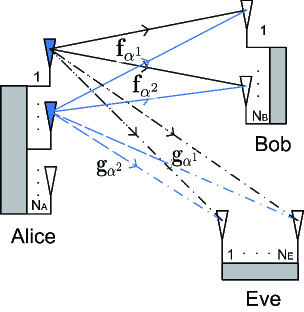
Fig. 1 depicts the MIMO wiretap channel of interest, where the transmitter (Alice), the receiver (Bob), and the eavesdropper (Eve) are equipped with , , and antennas, respectively. We assume that the main channel between Alice and Bob and the eavesdropper’s channel between Alice and Eve are subject to quasi-static Rayleigh fading. Under this assumption, the fading coefficients are invariant during two adjacent blocks of time durations within which the Alamouti scheme is applied. We also assume the same fading block length in the main channel and the eavesdropper’s channel. For such a wiretap channel, the passive eavesdropping scenario is considered where Eve overhears the transmission between Alice and Bob without inducing any interference to the main channel. In this scenario, the instantaneous channel state information (CSI) of the eavesdropper’s channel is not available at Alice. Of course, we preserve the assumption that Bob has the full CSI of the main channel and Eve has the full CSI of the eavesdropper’s channel.
We propose a TAS-Alamouti scheme to enhance the physical layer security in the MIMO wiretap channel of interest. Specifically, the proposed scheme is performed in two steps. We next detail the two steps, as follows:
II-1 First Step – TAS
In the first step, the first two strongest antennas out of antennas are selected at Alice. These two antennas maximize the instantaneous SNR between Alice and Bob. Here, Bob employs MRC to combine the received signals. As per this criterion, the index of the first strongest antenna is given by
| (1) |
and the index of the second strongest antenna is given by
| (2) |
In (1) and (2), we denote as the channel vector between the -th antenna at Alice and the antennas at Bob with independent and identically distributed (i.i.d.) Rayleigh fading entries.
To conduct antenna selection, Alice sends Bob pilot symbols prior to data transmission. Using these symbols, Bob precisely estimates the CSI of the main channel and determines and according to (1) and (2). After that, Bob feeds back and to Alice via a low-rate feedback channel. As such, our scheme reduces the feedback overhead compared with beamforming, since only a small number of bits are required to feedback the antenna indices. We note that the antenna indices (1) and (2) are entirely dependent on the main channel. As such, the two strongest transmit antennas for Bob corresponds to two random transmit antennas for Eve. It follows that our scheme improves the quality of main channel relative to the eavesdropper’s channel, which in turn promotes the secrecy of the wiretap channel.
II-2 Second Step – Alamouti
In the second step, Alice adopts the Alamouti scheme to perform secure transmission at the two selected antennas. After receiving the signals from Alice, Bob applies MRC to combine the received signals and maximize the SNR of the main channel. This allows Bob to exploit the -antenna diversity and maximize the probability of secure transmission. At the same time, Eve applies MRC to exploit the -antenna diversity and maximize the probability of successful eavesdropping.
As per the rules of the Alamouti scheme, the received signal vectors at Bob in the first and second time slots are given by
| (5) |
and
| (8) |
respectively, where is the main channel matrix after TAS, is the transmit signal vectors in the first time slot, is the transmit signal vectors in the second time slot, and is the zero-mean circularly symmetric complex Gaussian noise vector satisfying . Under the power constraint, we have , where is the total transmit power at Alice.
By performing MRC and space-time signal processing, the signals at Bob are expressed as
| (9) |
and
| (10) |
Since and are independent from each other, the instantaneous SNR at Bob for is identical to the instantaneous SNR at Bob for , which is written as
| (11) |
Following the same procedure as detailed above, the instantaneous SNR at Eve is written as
| (12) |
where is the eavesdropper’s channel matrix after TAS and denotes the channel vector between the -th antenna at Alice and the antennas at Eve with i.i.d. Rayleigh fading entries.
III Secrecy Performance of TAS-Alamouti
In this section, we concentrate on the secrecy performance of the proposed TAS-Alamouti scheme for non-identical Rayleigh fading between the main channel and the eavesdropper’s channel. Specifically, we derive a new closed-form expression for the secrecy outage probability. Based on this result, we express the probability of non-zero secrecy capacity in closed form and present the -outage secrecy capacity in integral form.
III-A Secrecy Outage Probability
The secrecy outage probability is defined as the probability of the secrecy capacity being less than a specific transmission rate (bits/channel) [10]. In the MIMO wiretap channel, is expressed as
| (13) |
where is the capacity of the main channel and is the capacity of the eavesdropper’s channel. Here, is the instantaneous SNR at Bob given by (11) and is the instantaneous SNR at Eve given by (12). According to the definition, the secrecy outage probability is formulated as
| (14) |
We commence our analysis by presenting the probability density functions (pdfs) of and . Specifically, we adopt [16, Eq. (15)] as the pdf of , , and define as the average per-antenna SNR at Bob. We note that and are equivalent to two random transmit antennas for Eve. As such, the pdf of , , is given by [16, Eq. (15)] with . We further define as the average per-antenna SNR at Eve.
We now proceed with the calculation of the secrecy outage probability. Specifically, we rewrite as
| (15) |
where is derived as
| (16) |
It is easy to observe that . As such, we simplify as .
| (13a) |
| (13b) |
| (13c) |
| (13d) |
To derive , we first calculate the inner integral with respect to by substituting and into and applying [17, Eq. (3.351.1)]. We then expand the product of the inner integral and by applying [17, Eq. (1.111)] and solve the resultant integral with respect to by applying [17, Eq. (3.351.3)]. By performing some algebraic manipulations, the secrecy outage probability is derived as
| (17) |
where , , and are presented in (III-A), (III-A), (III-A) and (III-A), respectively. In (III-A), (III-A), (III-A) and (III-A), we define variables , , , , , and . We also define the functions
and
We further define as the coefficients of for , which arises from the expansion of
| (18) |
and define for in and as
| (19) |
It is highlighted that our new expression in (17) is in closed form as it involves finite summations of exponential functions and power functions.
III-B Probability of Non-zero Secrecy Capacity
The probability of non-zero secrecy capacity is defined as the probability by which the secrecy capacity is larger than zero. As such, it is expressed as
| (20) |
Substituting and into (III-B) and solving the resultant integrals, the explicit expression for is obtained. Due to page limits, the explicit expression is omitted here. Instead, we present in terms of the secrecy outage probability as
| (21) |
III-C -Outage Secrecy Capacity
IV Numerical Results
In this section, we present numerical results to examine the impact of the number of antennas and the average SNRs on the secrecy performance. Specifically, we conduct a thorough performance comparison between our TAS-Alamouti scheme with the single TAS scheme in [12]. This comparison highlights the potential of TAS-Alamouti.
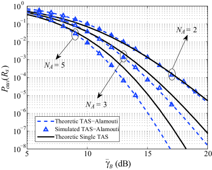
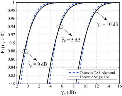
We first examine the impact of on the secrecy outage probability. Fig. 2 plots versus for different . In this figure, the theoretical TAS-Alamouti curve is generated from (17), and the theoretical single TAS curve is generated from [12, Eq. (13)]. We first observe that of TAS-Alamouti significantly decreases as increases. Moreover, we observe that TAS-Alamouti achieves a lower than single TAS when is in the medium and high regime. For example, TAS-Alamouti outperforms single TAS when dB for . This is due to the fact that more transmit energy is wasted on the second strongest antenna for Eve than for Bob at medium and high . Furthermore, we observe that TAS-Alamouti provides a higher than single TAS when is low. As such, it is easy to determine the crossover point at which TAS-Alamouti and single TAS achieve the same performance. Notably, we find that the value of at the crossover point decreases as increases. This can be explained by the fact that the two selected transmit antennas are determined by Bob and the freedom of increases with . Finally, we observe that the theoretical curves match precisely with the Monte Carlo simulations. This verifies the correctness of our analysis. Monte Carlo simulations are omitted in other figures to avoid cluttering.
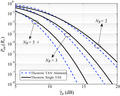
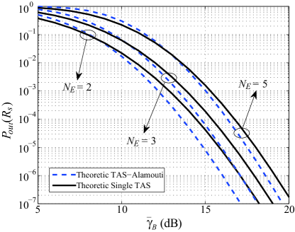
We next examine the impact of and on the secrecy outage probability. Fig. 3 plots versus for different . In this figure, we observe that of TAS-Alamouti profoundly decreases as increases. Moreover, we observe that the value of at the crossover point decreases as increases. This is due to the fact that larger increases the freedom of . Fig. 4 plots versus for different . In this figure, we observe that of TAS-Alamouti increases as increases. In addition, we observe that the value of at the crossover point increases as increases. This arises from the fact that larger increases the freedom of .
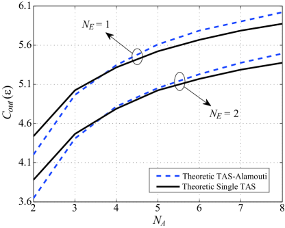
We now focus our attention on the probability of non-zero secrecy capacity. Fig. 5 plots versus for different . In this figure, the theoretical TAS-Alamouti curve is generated from (III-B), and the theoretical single TAS curve is generated from [12, Eq. (29)]. From Fig. 5, we see that the of TAS-Alamouti is higher than that of single TAS when is larger than a specific value. In particular, we observe that the value of at the crossover point is around . Notably, this value increases as increases. Additionally, we observe that of TAS-Alamouti still exists when .
Finally, we examine the -outage secrecy capacity. Fig. 6 plots versus for different . In this figure, the theoretical TAS-Alamouti curve is generated from (22), and the theoretical single TAS curve is generated from [12, Eq. (31)]. From this figure, we see that of TAS-Alamouti increases with but decreases with . We also see that TAS-Alamouti achieves a higher than single TAS when is larger than a certain value.
V Conclusion
In this work we have introduced a new TAS-Alamouti scheme for physical layer security enhancement in MIMO wiretap channels. Adopting non-identical Rayleigh fading between the main channel and the eavesdropper’s channel, we derived a new closed-form expression for the secrecy outage probability, based on which the probability of non-zero secrecy capacity and -outage secrecy capacity were characterized. We proved that the our TAS-Alamouti scheme achieves lower secrecy outage probability than the single TAS scheme when the SNR of the main channel is in the medium and high regime relative to the SNR of the eavesdropper’s channel. Future directions for our new scheme include its integration with location verification techniques [18][19] for even more enhanced security at the wireless physical layer.
Acknowledgments
This work was funded by The University of New South Wales and Australian Research Council Grant DP120102607.
References
- [1] Y.-S. Shiu, S. Y. Chang, H.-C. Wu, S. C.-H. Huang, and H.-H. Chen, “Physical layer security in wireless networks: A tutorial,” IEEE Commun. Mag., vol. 18, no. 5, pp. 66–74, Apr. 2011.
- [2] H. V. Poor, “Information and inference in the wireless physical layer,” IEEE Commun. Mag., vol. 19, no. 1, pp. 40–47, Feb. 2012.
- [3] C. E. Shannon, “Communication theory of secrecy systems,” Bell Syst. Techn. J., vol. 28, no. 4, pp. 656–715, Oct. 1949.
- [4] A. Wyner, “The wire-tap channel,” Bell Syst. Techn. J., vol. 54, no. 8, pp. 1355–1387, Oct. 1975.
- [5] S. K. Leung-Yan-Cheong and M. E. Hellman, “The Gaussian wire-tap channel,” IEEE Trans. Inf. Theory, vol. 24, no. 4, pp. 451–456, Jul. 1978.
- [6] A. Khisti and G. W. Wornell, “Secure transmission with multiple antennas–Part II: The MIMOME wiretap channel,” IEEE Trans. Inf. Theory, vol. 56, no. 11, pp. 5515–5532, Nov. 2010.
- [7] F. Oggier and B. Hassibi, “The secrecy capacity of the MIMO wiretap channel,” IEEE Trans. Inf. Theory, vol. 57, no. 8, pp. 4961–4972, Aug. 2011.
- [8] S. Goel and R. Negi, “Guaranteeing secrecy using artificial noise,” IEEE Trans. Wireless Commun., vol. 7, no. 6, pp. 2180–2189, Jun. 2008.
- [9] A. Mukherjee and A. L. Swindlehurst, “Robust beamforming for secrecy in MIMO wiretap channels with imperfect CSI,” IEEE Trans. Signal Process., vol. 59, no. 1, pp. 351–361, Jan. 2011.
- [10] M. Bloch, J. Barros, M. Rodrigues, and S. McLaughlin, “Wireless information-theoretic security,” IEEE Trans. Inf. Theory, vol. 54, no. 6, pp. 2515–2534, Jun. 2008.
- [11] H. Alves, R. D. Souza, M. Debbah, and M. Bennis, “Performance of transmit antenna selection physical layer security schemes,” IEEE Signal Process. Lett., vol. 19, no. 6, pp. 372–375, Jun. 2012.
- [12] N. Yang, P. L. Yeoh, M. Elkashlan, R. Schober, and I. B. Collings, “Secure transmission via transmit antenna selection in MIMO wiretap channels,” in Proc. IEEE GlobeCOM, Anaheim, CA, Dec. 2012, pp. 807–812.
- [13] N. Yang, P. L. Yeoh, M. Elkashlan, R. Schober, and I. B. Collings, “Transmit antenna selection for security enhancement in MIMO wiretap channels,” IEEE Trans. Commun., vol. 61, no. 1, pp. 144–154, Jan. 2013.
- [14] J. Yuan, “Adaptive transmit antenna selection with pragmatic space-time trellis codes,” IEEE Trans. Wireless Commun., vol. 5, no. 7, pp. 1706–1715, Jul. 2006.
- [15] S. Alamouti, “A simple transmit diversity technique for wireless communications,” IEEE J. Sel. Areas Commun., vol. 16, no. 8, pp. 1451–1458, Oct. 1998.
- [16] Z. Chen, J. Yuan, B. Vucetic, and Z. Zhou, “Performance of Alamouti scheme with transmit antenna selection,” Electron. Lett., vol. 39, pp. 1666–1668, Nov. 2003.
- [17] I. S. Gradshteyn and I. M. Ryzhik, Table of Integrals, Series and Products, 7th ed., Academic, San Diego, CA, 2007.
- [18] R. A. Malaney, “Securing Wi-Fi networks with position verification: extended version,” International J. Security Netw., vol. 2, pp. 27–36, Mar. 2007.
- [19] S. Yan, R. Malaney, I. Nevat, and G. Peters, “An information theoretic location verification system for wireless networks,” in Proc. IEEE GlobeCOM, Anaheim, CA, Dec. 2012, pp. 5637–5642.