The Johns Hopkins University

 

Estimating Confusions in the ASR Channel for
Improved Topic-based Language Model Adaptation

 

Damianos Karakos, Mark Dredze, Sanjeev Khudanpur

Technical Report 8

©HLTCOE, 2013

Acknowledgements This work is supported, in part, by the Human Language Technology Center of Excellence. Any opinions, findings, and conclusions or recommendations expressed in this material are those of the authors and do not necessarily reflect the views of the sponsor.

HLTCOE
810 Wyman Park Drive
Baltimore, Maryland 21211
http://hltcoe.jhu.edu

Abstract

Human language is a combination of elemental languages/domains/styles that change across and sometimes within discourses. Language models, which play a crucial role in speech recognizers and machine translation systems, are particularly sensitive to such changes, unless some form of adaptation takes place. One approach to speech language model adaptation is self-training, in which a language model’s parameters are tuned based on automatically transcribed audio. However, transcription errors can misguide self-training, particularly in challenging settings such as conversational speech. In this work, we propose a model that considers the confusions (errors) of the ASR channel. By modeling the likely confusions in the ASR output instead of using just the 1-best, we improve self-training efficacy by obtaining a more reliable reference transcription estimate. We demonstrate improved topic-based language modeling adaptation results over both 1-best and lattice self-training using our ASR channel confusion estimates on telephone conversations.

1 Introduction

Modern statistical automatic speech recognition (ASR) systems rely on language models for ranking hypotheses generated from acoustic data. Language models are trained on millions of words (or more) taken from text that matches the spoken language, domain and style of interest. Reliance on (static) training data makes language models brittle [Bellegarda, 2001] to changes in domain. However, for many problems of interest, there are numerous hours of spoken audio but little to no written text for language model training. In these settings, we must rely on language model adaptation using the spoken audio to improve performance on data of interest. One common approach to language model adaptation is self-training [Novotney et al., 2009], in which the language model is retrained on the output from the ASR system run on the new audio. Unfortunately, self-training learns from both correct and error ridden transcriptions that mislead the system, a particular problem for high word error rate (WER) domains, such as conversational speech. Even efforts to consider the entire ASR lattice in self-training cannot account for the ASR error bias. Worse still, this is particularly a problem for rare content words as compared to common function words; the fact that content words are more important for understandability exacerbates the problem.

Confusions in the ASR output pose problems for other applications, such as speech topic classification and spoken document retrieval. In high-WER scenarios, their performance degrades, sometimes considerably [Hazen and Richardson, 2008].

In this work, we consider the problem of topic adaptation of a speech recognizer [Seymore and Rosenfeld, 1997], in which we adapt the language model to the topic of the new speech. Our novelty lies in the fact that we correct for the biases present in the output by estimating ASR confusions. Topic proportions are estimated via a probabilistic graphical model which accounts for confusions in the transcript and provides a more accurate portrayal of the spoken audio. To demonstrate the utility of our model, we show improved results over traditional self-training as well as lattice based self-training for the challenging setting of conversational speech transcription. In particular, we show statistically significant improvements for content words.

Note that ?) also consider the problem of language model adaptation as an error correction problem, but with supervised methods. They train an error-correcting perceptron model on reference transcriptions from the new domain. In contrast, our approach does not assume the existence of transcribed data for training a confusion model; rather, the model is trained in an unsupervised manner based only on the ASR output.

The paper proceeds as follows: Section 2 describes our setting of language model adaptation and our topic based language model. Section 3 presents a language model adaptation process based on maximum-likelihood and maximum-aposteriori self-training, while Section 4 introduces adaptation that utilizes ASR channel estimates. Section 5 describes experiments on conversational speech.

2 Language Model Adaptation

We are given a trained speech recognizer, topic-based language model and a large collection of audio utterances (many conversations) for a new domain, i.e. a change of topics, but not manually transcribed text needed for language model training. Our goal is to adapt the language model by learning new topic distributions using the available audio. We consider self-training that adapts the topic distributions based on automatically transcribed audio.

A conversation ${\cal C}$ is composed of $N$ speech utterances are represented by $N$ lattices (confusion networks) – annotated with words and posterior probabilities – produced by the speech recognizer. Each confusion network consists of a sequence of bins, where each bin is a set of words hypothesized by the recognizer at a particular time. The $i$-th bin is denoted by $b_{i}$ and contains words $\{w_{i,j}\}_{j=1}^{|\cal{V}|}$, where ${\cal V}$ is the vocabulary. When obvious from context, we omit subscript $j$. The most likely word in bin $b_{i}$ is denoted by $\widehat{w}_{i}$. Let $M$ be the total number of bins in the $N$ confusion networks in a single conversation.

We use unigram topic-based language models (multinomial distributions over $\cal{V}$), which capture word frequencies under each topic. Such models have been used in a variety of ways, such as in PLSA [Hofmann, 2001] and LDA [Blei et al., 2003], and under different training scenarios. Topic-based models provide a global context beyond the local word history in modeling a word’s probability, and have been found especially useful in language model adaptation [Tam and Schultz, 2005, Wang and Stolcke, 2007, Hsu and Glass, 2006]. Each topic $t\in\{1,\ldots,T\}$ has a multinomial distribution denoted by $q(w|t),w\in{\cal V}$. These topic-word distributions are learned from conversations labeled with topics, such as those in the Fisher speech corpus.

Adapting the topic-based language model means learning a set of conversation specific mixture weights $\boldsymbol{\lambda}^{\cal C}=(\lambda_{1}^{\cal C},\ldots,\lambda_{T}^{\cal C})$, where $\lambda_{t}^{\cal C}$ indicates the likelihood of seeing topic $t$ in conversation ${\cal C}$. While topic compositions remain fixed, the topics selected change with each conversation. These mixture weights form the true distribution of a word:

$$q(w)=\sum_{t=1}^{T}\lambda_{t}q(w|t).$$ (1)

3 Learning $\boldsymbol{\lambda}$ from ASR Output

We begin by following previous approaches to self-training, in which model parameters are re-estimated based on ASR output. We consider self-training based on 1-best and lattice maximum-likelihood estimation (MLE) as well as maximum-aposteriori (MAP) training. In the next section, we modify these approaches to incorporate our confusion estimates.

For estimating the topic mixtures $\boldsymbol{\lambda}$ using self-training on the 1-best ASR output, i.e. the 1-best path in the confusion network $\mathbf{\widehat{w}}=\{\widehat{w}_{i}\}_{i=1}^{M}$, we write the log-likelihood of the observations $\mathbf{\widehat{w}}$:

$${\cal L}^{(1)}=\sum_{i=1}^{M}\log q(\widehat{w}_{i}),$$ (2)

where $q$ is a mixture of topic models (1), for mixture weights $\boldsymbol{\lambda}$. We expect topic-based distributions will better estimate the true word distribution than the empirical estimate $\hat{q}(w)=\frac{1}{M}\sum_{i=1}^{M}\boldsymbol{1}(\widehat{w}_{i}=w),$ as the latter is biased due to ASR errors. Maximum-likelihood estimation of $\boldsymbol{\lambda}$ in (2) is given by:

$$\boldsymbol{\lambda}^{*} = \arg\max_{\boldsymbol{\lambda}}\sum_{i=1}^{M}\log q(\widehat{w}_{i})$$ (3)

$$= \arg\max_{\boldsymbol{\lambda}}\sum_{i=1}^{M}\log\left(\sum_{t}\lambda_{t}q(\widehat{w}_{i}|t)\right)$$

Using the EM algorithm, $Q$ is the expected log-likelihood of the “complete” data:

$$Q(\boldsymbol{\lambda}^{(j)},\boldsymbol{\lambda})=\sum_{i=1}^{M}\sum_{t}r^{(j)}(t|\widehat{w}_{i})\log(\lambda_{t}q(\widehat{w}_{i}|t)),$$ (4)

where $r^{(j)}(t|\widehat{w}_{i})$ is the posterior distribution of the topic in the $i$-th bin, given the 1-best word $\widehat{w}_{i}$; this is computed in the E-step of the $j$-th iteration:

$$r^{(j)}(t|\widehat{w}_{i})=\frac{\lambda_{t}^{(j)}q(\widehat{w}_{i}|t)}{\sum_{t^{\prime}}\lambda_{t^{\prime}}^{(j)}q(\widehat{w}_{i}|t^{\prime})}.$$ (5)

In the M-step of the $j+1$ iteration, the new estimate of the prior is computed by maximizing (4), i.e.,

$$\lambda_{t}^{(j+1)}=\frac{\sum_{i=1}^{M}r^{(j)}(t|\widehat{w}_{i})}{\sum_{t^{\prime}}\sum_{i^{\prime}=1}^{M}r^{(j)}(t^{\prime}|\widehat{w}_{i^{\prime}})}.$$ (6)

3.1 Learning $\boldsymbol{\lambda}$ from Expected Counts

Following ?) we next consider using the entire bin in self-training by maximizing the expected log-likelihood of the ASR output:

$${\cal L}^{\prime(1)}=E\left[\sum_{i=1}^{M}\log q(W_{i})\right],$$ (7)

where $W_{i}$ is a random variable which takes the value $w\in b_{i}$ with probability equal to the confidence (posterior probability) $s_{i}(w)$ of the recognizer. The maximum-likelihood estimation problem becomes:

$$\boldsymbol{\lambda}^{*}\! \!\!\!\!=\!\!\!\! \arg\max_{\boldsymbol{\lambda}}{\cal L}^{\prime(1)}$$

$$\!\!\!\!=\!\!\!\! \arg\max_{\boldsymbol{\lambda}}\sum_{i=1}^{M}\sum_{w\in b_{i}}s_{i}(w)\log\left(\sum_{t}\lambda_{t}q(w|t)\right)$$

$$\!\!\!\!=\!\!\!\! \arg\max_{\boldsymbol{\lambda}}\sum_{w\in{\cal V}}\text{\em tf}(w)\log\left(\sum_{t}\lambda_{t}q(w|t)\right)$$

where $\text{\em tf}(w)=\sum_{i}s_{i}(w)$ denotes the expected count of word $w$ in the conversation, given by the sum of the posteriors of $w$ in all the confusion network bins of the conversation [Karakos et al., 2011] (note that for text documents, it is equivalent to term-frequency). We again use the EM algorithm, with objective function:

$$Q(\boldsymbol{\lambda}^{(j)},\boldsymbol{\lambda})=\sum_{w\in{\cal V}}\text{\em tf}(w)\sum_{t}r^{(j)}(t|w)\log(\lambda_{t}q(w|t)),$$ (9)

where $r^{(j)}(t|w)$ is the posterior distribution of the topic given word $w$ computed using (5) (but with $w$ instead of $\widehat{w}_{i}$). In the M-step of the $j+1$ iteration, the new estimate of the prior is computed by maximizing (9), i.e.,

$$\lambda_{t}^{(j+1)}=\frac{\sum_{w\in{\cal V}}\text{\em tf}(w)r^{(j)}(t|w)}{\sum_{t^{\prime}}\sum_{w\in{\cal V}}\text{\em tf}(w)r^{(j)}(t^{\prime}|w)}.$$ (10)

3.2 Maximum-Aposteriori Estimation of $\boldsymbol{\lambda}$

In addition to a maximum likelihood estimate, we consider a maximum-aposteriori (MAP) estimate by placing a Dirichlet prior over $\boldsymbol{\lambda}$ [Bacchiani and Roark, 2003]:

$$\boldsymbol{\lambda}^{*}=\arg\max_{\boldsymbol{\lambda}}{\cal L}+\beta\log(\text{Dir}(\boldsymbol{\lambda};\alpha))$$ (11)

where $\text{Dir}(\boldsymbol{\lambda};\alpha)$ is the pdf of the Dirichlet distribution with parameter $\alpha$: $\text{Dir}(\boldsymbol{\lambda};\alpha)=\frac{1}{B(\alpha)}\prod_{t}\lambda_{t}^{\alpha-1}.$

This introduces an extra component in the optimization. It is easy to prove that the update equation for $\lambda_{t}^{(j+1)}$ becomes:

$$\lambda_{t}^{(j+1)}\!=\!\left[\frac{\sum_{i=1}^{M}r^{(j)}(t|\widehat{w}_{i})+\beta(\alpha-1)}{\sum_{t^{\prime}}\sum_{i=1}^{M}r^{(j)}(t^{\prime}|\widehat{w}_{i})+T\beta(\alpha-1)}\right]_{+}.$$ (12)

for the case where only the ASR 1-best is used, and

$$\lambda_{t}^{(j+1)}\!=\!\left[\frac{\sum_{w\in{\cal V}}\text{\em tf}(w)r^{(j)}(t|w)+\beta(\alpha-1)}{\sum_{t^{\prime}}\sum_{w\in{\cal V}}\text{\em tf}(w)r^{(j)}(t^{\prime}|w)+T\beta(\alpha-1)}\right]_{+}.$$ (13)

for the case where expected counts are used. Note that the $[x]_{+}$ notation stands for $\max\{0,x\}$.

4 Confusion Estimation in ASR Output

Figure 1: The graphical model representations for maximum-likelihood 1-best self-training (left), self-training with the ASR channel confusion model (middle), MAP training with the confusion model (right). In all models, each word is conditionally independent given the selected topic, and topic proportions $\boldsymbol{\lambda}$ are conversation specific. For the middle and right models, each observed top word in the $i$-th confusion network bin ($\widehat{w}_{i}$) is generated by first sampling a topic $t_{i}$ according to $\boldsymbol{\lambda}$, then sampling the (true) word $w_{i}$ according to the topic $t_{i}$, and finally sampling the observed ASR word $\widehat{w}_{i}$ based on the ASR channel confusion model ($p_{c}(v|w)$). For expected count models, $\widehat{w}_{i}$ becomes a distribution over words in the confusion network bin $b_{i}$.

Self-training on ASR output can mislead the language model through confusions in the ASR channel. By modeling these confusions we can guide self-training and recover from recognition errors.

The ASR channel confusion model is represented by a conditional probability distribution $p_{c}(v|w),v,w\in{\cal V}$, which denotes the probability that the most likely word in the output of the recognizer (i.e., the “1-best” word) is $v$, given that the true (reference) word spoken is $w$. Of course, this conditional distribution is just an approximation as many other phenomena – coarticulation, non-stationarity of speech, channel variations, lexical choice in the context, etc. – cause this probability to vary. We assume that $p_{c}(v|w)$ is an “average” of the conditional probabilities under various conditions.

We use the following simple procedure for estimating the ASR channel, similar to that of [Xu et al., 2009] for computing cohort sets:

• Create confusion networks [Mangu et al., 1999] with the available audio.

• Count $c(w,v)$, the number of times words $w,v$ appear in the same bin.

• The conditional ASR probability is computed as $p_{c}(v|w)=c(v,w)/\sum_{v^{\prime}}c(v^{\prime},w)$.

• Prune words whose posterior probabilities are lower than 5% of the max probability in a bin.

• Keep only the top 10 words in each bin.

The last two items above were implemented as a way of reducing the search space and the complexity of the task. We did not observe significant changes in the results when we relaxed these two constraints.

4.1 Learning $\boldsymbol{\lambda}$ with ASR Confusion Estimates

We now derive a maximum-likelihood estimate of $\boldsymbol{\lambda}$ based on the 1-best ASR output but relies on the ASR channel confusion model $p_{c}$. The log-likelihood of the observations (most likely path in the confusion network) is:

$${\cal L}^{(2)}=\sum_{i=1}^{M}\log p(\widehat{w}_{i}),$$ (14)

where $p$ is the induced distribution on the observations under the confusion model $p_{c}(v|w)$ and the estimated distribution $q$ of (1):

$$p(\widehat{w}_{i})=\sum_{w\in\cal{V}}q(w)p_{c}(\widehat{w}_{i}|w).$$ (15)

Recall that while we sum over $\cal{V}$, in practice the summation is limited to only likely words. One could argue that the ASR channel confusion distribution $p_{c}(\widehat{w}_{i}|w)$ should discount unlikely confusions. However, since $p_{c}$ is not bin specific, unlikely words in a specific bin could receive non-negligible probability from $p_{c}$ if they are likely in general. This makes the truncated summation over $\cal{V}$ problematic.

One solution would be to reformulate $p_{c}(\widehat{w}_{i}|w)$ so that it becomes a conditional distribution given the left (or even right) lexical context of the bin. But this formulation adds complexity and suffers from the usual sparsity issues. The solution we follow here imposes the constraint that only the words already existing in $b_{i}$ are allowed to be candidate words giving rise to $\widehat{w}_{i}$. This uses the “pre-filtered” set of words in $b_{i}$ to condition on context (acoustic and lexical), without having to model such context explicitly. We anticipate that this conditioning on the words of $b_{i}$ leads to more accurate inference. The likelihood objective then becomes:

$${\cal L}^{\prime(2)}=\sum_{i=1}^{M}\log p_{i}(\widehat{w}_{i}),$$ (16)

with $p_{i}$ defined as:

$$p_{i}(\widehat{w}_{i})=\sum_{w\in b_{i}}\frac{q(w)}{\sum_{w^{\prime}\in b_{i}}q(w^{\prime})}p_{c}(\widehat{w}_{i}|w),$$ (17)

i.e., the induced probability conditioned on bin $b_{i}$. Note that although we estimate a conversation level distribution $q(w)$, it has to be normalized in each bin by dividing by $\sum_{w\in b_{i}}q(w)$, in order to condition only on the words in the bin. The maximum-likelihood estimation for $\boldsymbol{\lambda}$ becomes:

$$\mspace{-170.0mu}\boldsymbol{\lambda}^{*}=\arg\max_{\boldsymbol{\lambda}}{\cal L}^{\prime(2)} =\arg\max_{\boldsymbol{\lambda}}\sum_{i=1}^{M}\log p_{i}(\widehat{w}_{i})$$

$$\mspace{-170.0mu}=\arg\max_{\boldsymbol{\lambda}}\sum_{i=1}^{M}\log\left(\sum_{w\in b_{i}}\frac{\sum_{t}\lambda_{t}q(w|t)p_{c}(\widehat{w}_{i}|w)}{\sum_{w^{\prime}\in b_{i}}\sum_{t^{\prime}}\lambda_{t^{\prime}}q(w^{\prime}|t^{\prime})}\right)$$

(18)

Note that the appearance of $\lambda_{t}$ in the denominator makes the maximization harder.

As before, we rely on an EM-procedure to maximize this objective. Let us assume that at the $j$-th iteration of EM we have an estimate of the prior distribution $q$, denoted by $q^{(j)}$. This induces an observation probability in bin $i$ based on equation (17), as well as a posterior probability $r_{i}^{(j)}(w|\widehat{w}_{i})$ that a word $w\in b_{i}$ is the reference word, given $\widehat{w}_{i}$. The goal is to come up with a new estimate of the prior distribution $q^{(j+1)}$ that increases the value of the log-likelihood. If we define:

$$Q(q^{(j)},q^{\prime})=$$

$$= \!\!\!\!\sum_{i=1}^{M}\sum_{w\in b_{i}}r_{i}^{(j)}(w|\widehat{w}_{i})\log(p_{c}(\widehat{w}_{i}|w)q_{i}^{\prime}(w))$$

$$= \!\!\!\!\sum_{i=1}^{M}\sum_{w\in b_{i}}r_{i}^{(j)}(w|\widehat{w}_{i})\log\left(\frac{p_{c}(\widehat{w}_{i}|w)q^{\prime}(w)}{\sum_{w^{\prime}\in b_{i}}q^{\prime}(w^{\prime})}\right)$$

then we have:

$${\cal L}^{\prime(2)}(q^{(j)},q^{\prime})-{\cal L}^{\prime(2)}(q^{(j)},q^{(j)})$$ (20)

$$= Q(q^{(j)},q^{\prime})-Q(q^{(j)},q^{(j)})$$

$$+\sum_{i=1}^{M}D(r_{i}^{(j)}(\cdot|\widehat{w}_{i})\|r_{i}^{\prime}(\cdot|\widehat{w}_{i}))$$

$$\geq Q(q^{(j)},q^{\prime})-Q(q^{(j)},q^{(j)})~{},$$

where (20) holds because $D(r_{i}^{(j)}(\cdot|\widehat{w}_{i})\|r_{i}^{\prime}(\cdot|\widehat{w}_{i}))\geq 0$ [Cover and Thomas, 1996]. Thus, we just need to find the value of $q^{\prime}$ that maximizes $Q(q^{(j)},q^{\prime})$, as this will guarantee that ${\cal L}^{\prime(2)}(q^{(j)},q^{\prime})\geq{\cal L}^{\prime(2)}(q^{(j)},q^{(j)})$. The distribution $q^{\prime}$ can be written:

$$q^{\prime}(w)=\sum_{t}\lambda_{t}q(w|t).$$ (21)

Thus, $Q$, as a function of $\boldsymbol{\lambda}$, can be written as:

$$Q(q^{(j)},\boldsymbol{\lambda})=$$

$$\mspace{-40.0mu}\sum_{i=1}^{M}\sum_{w\in b_{i}}r_{i}^{(j)}(w|\widehat{w}_{i})\log\left(\frac{p_{c}(\widehat{w}_{i}|w)\sum_{t}\lambda_{t}q(w|t)}{\sum_{w^{\prime}\in b_{i}}\sum_{t}\lambda_{t}q(w^{\prime}|t)}\right).$$

Equation (LABEL:eq:q2) cannot be easily maximized with respect to $\boldsymbol{\lambda}$ by simple differentiation, because the elements of $\boldsymbol{\lambda}$ appear in the denominator, making them coupled. Instead, we will derive and maximize a lower bound for the $Q$-difference (20).

For the rest of the derivation we assume that $\lambda_{t}=\frac{e^{\mu_{t}}}{\sum_{t^{\prime}}e^{\mu_{t^{\prime}}}}$, where $\mu_{t}\in{\cal R}$. We can thus express $Q$ as a function of $\boldsymbol{\mu}=(\mu_{1},\ldots,\mu_{T})$ as follows:

$$Q(q^{(j)},\boldsymbol{\mu})=$$

$$\mspace{-35.0mu}\sum_{i=1}^{M}\sum_{w\in b_{i}}r_{i}^{(j)}(w|\widehat{w}_{i})\log\left(\frac{p_{c}(\widehat{w}_{i}|w)\sum_{t}\frac{e^{\mu_{t}}}{\sum_{t^{\prime}}e^{\mu_{t^{\prime}}}}q(w|t)}{\sum_{w^{\prime}\in b_{i}}\sum_{t}\frac{e^{\mu_{t}}}{\sum_{t^{\prime}}e^{\mu_{t^{\prime}}}}q(w^{\prime}|t)}\right)\mspace{-200.0mu}$$

$$\mspace{-20.0mu}= \mspace{-15.0mu}\sum_{i=1}^{M}\sum_{w\in b_{i}}r_{i}^{(j)}(w|\widehat{w}_{i})\log\left(\frac{p_{c}(\widehat{w}_{i}|w)\sum_{t}e^{\mu_{t}}q(w|t)}{\sum_{w^{\prime}\in b_{i}}\sum_{t}e^{\mu_{t}}q(w^{\prime}|t)}\right)$$

Interestingly, the fact that the sum $\sum_{t}e^{\mu_{t}}$ appears in both numerator and denominator in the above expression allows us to discard it.

At iteration $j+1$, the goal is to come up with an update $\boldsymbol{\delta}$, such that $\boldsymbol{\mu}^{(j)}+\boldsymbol{\delta}$ results in a higher value for $Q$; i.e., we require:

$$Q(q^{(j)},\boldsymbol{\mu}^{(j)}+\boldsymbol{\delta})\geq Q(q^{(j)},\boldsymbol{\mu}^{(j)}),$$ (24)

where $\boldsymbol{\mu}^{(j)}$ is the weight vector that resulted after optimizing $Q$ in the $j$-th iteration. Obviously,

$$q^{(j)}(w)=\sum_{t}\frac{e^{\mu_{t}^{(j)}}q(w|t)}{\sum_{t^{\prime}}e^{\mu_{t^{\prime}}^{(j)}}}.$$ (25)

Let us consider the difference:

$$Q(q^{(j)},\boldsymbol{\mu}^{(j)}+\boldsymbol{\delta})-Q(q^{(j)},\boldsymbol{\mu}^{(j)})$$ (27)

$$= \sum_{i=1}^{M}\sum_{w\in b_{i}}r_{i}^{(j)}(w|\widehat{w}_{i})\times$$

$$\Bigg{[}-\log\left(\frac{\sum_{t}e^{\mu_{t}^{(j)}+\delta_{t}}\sum_{w^{\prime}\in b_{i}}q(w^{\prime}|t)}{\sum_{t}e^{\mu_{t}^{(j)}}\sum_{w^{\prime}\in b_{i}}q(w^{\prime}|t)}\right)$$

$$+\log\left(\frac{\sum_{t}e^{\mu_{t}^{(j)}+\delta_{t}}q(w|t)}{\sum_{t}e^{\mu_{t}^{(j)}}q(w|t)}\right)\Bigg{]}~{}.$$

We use the well-known inequality $\log(x)\leq x-1\Rightarrow-\log(x)\geq 1-x$ and obtain:

$$-\log\left(\frac{\sum_{t}e^{\mu_{t}^{(j)}+\delta_{t}}\sum_{w^{\prime}\in b_{i}}q(w^{\prime}|t)}{\sum_{t}e^{\mu_{t}^{(j)}}\sum_{w^{\prime}\in b_{i}}q(w^{\prime}|t)}\right)\geq$$ (28)

$$1-\frac{\sum_{t}e^{\mu_{t}^{(j)}+\delta_{t}}\sum_{w^{\prime}\in b_{i}}q(w^{\prime}|t)}{\sum_{t}e^{\mu_{t}^{(j)}}\sum_{w^{\prime}\in b_{i}}q(w^{\prime}|t)}.$$

Next, we apply Jensen’s inequality to obtain:

$$\log\left(\frac{\sum_{t}e^{\mu_{t}^{(j)}+\delta_{t}}q(w|t)}{\sum_{t}e^{\mu_{t}^{(j)}}q(w|t)}\right)\geq\frac{\sum_{t}e^{\mu_{t}^{(j)}}q(w|t)\delta_{t}}{\sum_{t}e^{\mu_{t}^{(j)}}q(w|t)}.$$ (29)

By combining (27), (28) and (29), we obtain a lower bound on the $Q$-difference of (27):

$$Q(q^{(j)},\boldsymbol{\mu}^{(j)}+\boldsymbol{\delta})-Q(q^{(j)},\boldsymbol{\mu}^{(j)})\geq$$ (30)

$$\mspace{-35.0mu}\sum_{i=1}^{M}\sum_{w\in b_{i}}r_{i}^{(j)}(w|\widehat{w}_{i})\Bigg{[}1+\frac{\sum_{t}e^{\mu_{t}^{(j)}}q(w|t)\delta_{t}}{\sum_{t}e^{\mu_{t}^{(j)}}q(w|t)}$$

$$\mspace{-35.0mu}-\frac{\sum_{t}e^{\mu_{t}^{(j)}+\delta_{t}}\sum_{w^{\prime}\in b_{i}}q(w^{\prime}|t)}{\sum_{t}e^{\mu_{t}^{(j)}}\sum_{w^{\prime}\in b_{i}}q(w^{\prime}|t)}\Bigg{]}~{}.$$

It now suffices to find a $\boldsymbol{\delta}$ that maximizes the lower bound of (30), as this will guarantee that the $Q$-difference will be greater than zero. Note that the lower bound in (30) is a concave function of $\delta_{t}$, and it thus has a global maximum that we will find using differentiation. Let us set $g(\boldsymbol{\delta})$ equal to the right-hand-side of (30). Then,

$$\frac{\partial g(\boldsymbol{\delta})}{\partial\delta_{t}}=\sum_{i=1}^{M}\sum_{w\in b_{i}}r_{i}^{(j)}(w|\widehat{w}_{i})\times$$

$$\mspace{-35.0mu}\left[-\frac{e^{\mu_{t}^{(j)}+\delta_{t}}\sum_{w^{\prime}\in b_{i}}q(w^{\prime}|t)}{\sum_{t^{\prime}}e^{\mu_{t^{\prime}}^{(j)}}\sum_{w^{\prime}\in b_{i}}q(w^{\prime}|t^{\prime}))}+\frac{e^{\mu_{t}^{(j)}}q(w|t)}{\sum_{t^{\prime}}e^{\mu_{t^{\prime}}^{(j)}}q(w|t^{\prime})}\right].$$

(31)

By setting (31) equal to 0 and solving for $\delta_{t}$, we obtain the update for $\delta_{t}$ (or, equivalently, $e^{\mu_{t}^{(j)}+\delta_{t}}$):

$$\mspace{-40.0mu}e^{\mu_{t}^{(j)}+\delta_{t}}=\Bigg{(}\sum_{i=1}^{M}\sum_{w\in b_{i}}\frac{r_{i}^{(j)}(w|\widehat{w}_{i})e^{\mu_{t}^{(j)}}q(w|t)}{\sum_{t^{\prime}}e^{\mu_{t^{\prime}}^{(j)}}q(w|t^{\prime})}\Bigg{)}$$ (32)

$$\mspace{-40.0mu}\times\Bigg{(}\sum_{i=1}^{M}\frac{\sum_{w\in b_{i}}q(w|t)}{\sum_{t^{\prime}}e^{\mu_{t^{\prime}}^{(j)}}\sum_{w\in b_{i}}q(w|t^{\prime})}\Bigg{)}^{\!\!-1}$$

4.2 Learning $\boldsymbol{\lambda}$ from Expected Counts

As before, we now consider maximizing the expected log-likelihood of the ASR output:

$${\cal L}^{\prime\prime(2)}=E\left[\sum_{i=1}^{M}\log p(W_{i})\right],$$ (33)

where $W_{i}$ takes the value $w\in b_{i}$ with probability equal to the confidence (posterior probability) $s_{i}(w)$ of the recognizer. The modified maximum-likelihood estimation problem now becomes:

$$\mspace{0.0mu}\boldsymbol{\lambda}^{*}=\arg\max_{\boldsymbol{\lambda}}{\cal L}^{\prime\prime(2)}$$

$$\mspace{0.0mu}=\arg\max_{\boldsymbol{\lambda}}\sum_{i=1}^{M}\sum_{w\in b_{i}}s_{i}(w)\log p_{i}(w)$$

$$\mspace{0.0mu}=\arg\max_{\boldsymbol{\lambda}}\sum_{i=1}^{M}\sum_{w\in b_{i}}s_{i}(w)\times$$

$$\log\left(\sum_{w^{\prime}\in b_{i}}\frac{\sum_{t}\lambda_{t}q(w^{\prime}|t)p_{c}(w|w^{\prime})}{\sum_{w^{\prime\prime}\in b_{i}}\sum_{t^{\prime}}\lambda_{t^{\prime}}q(w^{\prime\prime}|t^{\prime})}\right)~{}.$$

(34)

By following a procedure similar to the one described earlier in this section, we come up with the lower bound on the $Q$-difference:

$$Q(q^{(j)},\boldsymbol{\mu}^{(j)}+\boldsymbol{\delta})-Q(q^{(j)},\boldsymbol{\mu}^{(j)})\geq$$ (35)

$$\mspace{-35.0mu}\sum_{i=1}^{M}\sum_{w,w^{\prime}\in b_{i}}r_{i}^{(j)}(w|w^{\prime})s_{i}(w^{\prime})\Bigg{[}1+\frac{\sum_{t}e^{\mu_{t}^{(j)}}q(w|t)\delta_{t}}{\sum_{t}e^{\mu_{t}^{(j)}}q(w|t)}$$

$$\mspace{-35.0mu}-\frac{\sum_{t}e^{\mu_{t}^{(j)}+\delta_{t}}\sum_{w^{\prime}\in b_{i}}q(w^{\prime}|t)}{\sum_{t}e^{\mu_{t}^{(j)}}\sum_{w^{\prime}\in b_{i}}q(w^{\prime}|t)}\Bigg{]}$$

whose optimization results in the following update equation for $\delta_{t}$:

$$\mspace{0.0mu}e^{\mu_{t}^{(j)}+\delta_{t}}=$$ (36)

$$\Bigg{(}\sum_{i=1}^{M}\sum_{w,w^{\prime}\in b_{i}}\frac{r_{i}^{(j)}(w|w^{\prime})s_{i}(w^{\prime})e^{\mu_{t}^{(j)}}q(w|t)}{\sum_{t^{\prime}}e^{\mu_{t^{\prime}}^{(j)}}q(w|t^{\prime})}\Bigg{)}$$

$$\mspace{0.0mu}\times\Bigg{(}\sum_{i=1}^{M}\frac{\sum_{w\in b_{i}}q(w|t)}{\sum_{t^{\prime}}e^{\mu_{t^{\prime}}^{(j)}}\sum_{w\in b_{i}}q(w|t^{\prime})}\Bigg{)}^{\!\!-1}~{}.$$

4.3 Maximum-Aposteriori Estimation of $\boldsymbol{\lambda}$

Finally, we consider a MAP estimation of $\boldsymbol{\lambda}$ with the confusion model. The optimization contains the term $\beta\log(\text{Dir}(\boldsymbol{\lambda};\alpha))$ and the $Q$-difference (20) is:

$$Q(q^{(j)},\boldsymbol{\mu}^{(j)}+\boldsymbol{\delta})-Q(q^{(j)},\boldsymbol{\mu}^{(j)})+$$

$$\beta\log(\text{Dir}(e^{\boldsymbol{\mu}^{(j)}+\boldsymbol{\delta}}/Z_{1}))-\beta\log(\text{Dir}(e^{\boldsymbol{\mu}^{(j)}}/Z_{0}))$$

where $Z_{0},Z_{1}$ are the corresponding normalizing constants. In order to obtain a lower bound on the difference in the second line of (LABEL:eq:q_diff_map), we consider the following chain of equalities:

$$\log(\text{Dir}(e^{\boldsymbol{\mu}^{(j)}+\boldsymbol{\delta}}/Z_{1}))-\log(\text{Dir}(e^{\boldsymbol{\mu}^{(j)}}/Z_{0}))=$$ (38)

$$\mspace{-30.0mu}=(\alpha-1)\sum_{t}\log\left(\frac{e^{\mu_{t}^{(j)}+\delta_{t}}/e^{\mu_{t}^{(j)}}}{\left(\sum_{t^{\prime}}e^{\mu_{t^{\prime}}^{(j)}+\delta_{t^{\prime}}}\right)/\left(\sum_{t^{\prime}}e^{\mu_{t}^{(j)}}\right)}\right)$$

$$\mspace{-30.0mu}=(\alpha-1)\left[\sum_{t}\delta_{t}-T\log\left(\sum_{t}\frac{e^{\mu_{t}^{(j)}}}{\sum_{t^{\prime}}e^{\mu_{t^{\prime}}^{(j)}}}e^{\delta_{t}}\right)\right]$$

We distinguish two cases:
(i) Case 1: $\alpha<1$.
We apply Jensen’s inequality to obtain the following lower bound on (38),

$$(\alpha-1)\left[\sum_{t}\delta_{t}-T\sum_{t}\frac{e^{\mu_{t}^{(j)}}}{\sum_{t^{\prime}}e^{\mu_{t^{\prime}}^{(j)}}}\delta_{t}\right]$$

$$=(\alpha-1)\left[\sum_{t}\delta_{t}-T\sum_{t}\lambda_{t}^{(j)}\delta_{t}\right]~{}.$$ (39)

The lower bound (39) now becomes part of the lower bound in (30) (for the case of the 1-best) or the lower bound (35) (for the case of expected counts), and after differentiating with respect to $\delta_{t}$ and setting the result equal to zero we obtain the update equation:

$$\mspace{0.0mu}e^{\mu_{t}^{(j)}+\delta_{t}}=(A+\beta(\alpha-1)(1-T\lambda_{t}^{(j)}))\times$$ (40)

$$\Bigg{(}\sum_{i=1}^{M}\frac{\sum_{w\in b_{i}}q(w|t)}{\sum_{t^{\prime}}e^{\mu_{t^{\prime}}^{(j)}}\sum_{w\in b_{i}}q(w|t^{\prime})}\Bigg{)}^{\!\!-1}$$

where $A$ in (40) is equal to

$$\sum_{i=1}^{M}\sum_{w\in b_{i}}\frac{r_{i}^{(j)}(w|\widehat{w}_{i})e^{\mu_{t}^{(j)}}q(w|t)}{\sum_{t^{\prime}}e^{\mu_{t^{\prime}}^{(j)}}q(w|t^{\prime})}$$ (41)

in the case of using just the 1-best, and

$$\sum_{i=1}^{M}\sum_{w,w^{\prime}\in b_{i}}\frac{r_{i}^{(j)}(w|w^{\prime})s_{i}(w^{\prime})e^{\mu_{t}^{(j)}}q(w|t)}{\sum_{t^{\prime}}e^{\mu_{t^{\prime}}^{(j)}}q(w|t^{\prime})}~{}.$$ (42)

in the case of using the lattice.
(ii) Case 2: $\alpha\geq 1$.
We apply the well-known inequality $\log(x)\leq x-1$ and obtain the following lower bound on (38),

$$(\alpha-1)\left[\sum_{t}\delta_{t}-T\left(\sum_{t}\frac{e^{\mu_{t}^{(j)}+\delta_{t}}}{\sum_{t^{\prime}}e^{\mu_{t^{\prime}}^{(j)}}}-1\right)\right]$$ (43)

As before, the lower bound (43) now becomes part of the lower bound in (30) (for the case of the 1-best) or the lower bound (35) (for the case of expected counts), and after differentiating with respect to $\delta_{t}$ and setting the result equal to zero we obtain the update equation:

$$\mspace{0.0mu}e^{\mu_{t}^{(j)}+\delta_{t}}=(A+\beta(\alpha-1))\times$$ (44)

$$\mspace{-40.0mu}\times\Bigg{(}\sum_{i=1}^{M}\frac{\sum_{w\in b_{i}}q(w|t)}{\sum_{t^{\prime}}e^{\mu_{t^{\prime}}^{(j)}}\sum_{w\in b_{i}}q(w|t^{\prime})}-\frac{\beta(\alpha-1)T}{\sum_{t^{\prime}}e^{\mu_{t^{\prime}}^{(j)}}}\Bigg{)}^{\!\!-1}$$

where $A$ in (44) is equal to (41) or (42), depending on whether the log-likelihood of the 1-best or the expected log-likelihood is maximized.

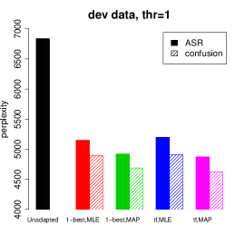
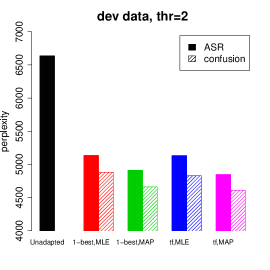
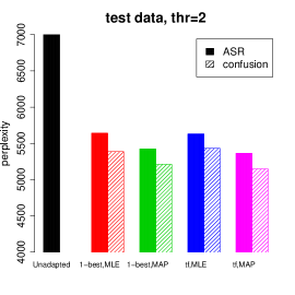
Figure 2: Perplexities of each language model. “Content-word” perplexity is computed over those words whose reference transcript counts do not exceed the threshold thr (shown at the top of each plot). We consider MLE and MAP solutions based on 1-best and expected counts (tf) for both ASR output self-training (solid bars) and our confusion model (dashed bars). Overall perplexity (which is dominated by function words) is not affected significantly.

Summary:

We summarize our methods as graphical models in Figure 1. We estimate the topic distributions $\boldsymbol{\lambda}^{\cal{C}}$ for a conversation $\cal{C}$ by either self-training directly on the ASR output, or including our ASR channel confusion model. For training on the ASR output, we rely on MLE 1-best training ((5),(6), left figure), or expected counts from the lattices (10). For both settings we also consider MAP estimation: 1-best (12) and expected counts (13). When using the ASR channel confusion model, we derived parallel cases for MLE 1-best ((32), middle figure) and expected counts (36), as well as the MAP (right figure) training of each ((41),(42)).

5 Experimental Results

We compare self-training, as described in Section 3, with our confusion approach, as described in Section 4, on topic-based language model adaptation.

Setup

Speech data is taken from the Fisher telephone conversation speech corpus, which has been split into 4 parts: set $A_{1}$ is one hour of speech used for training the ASR system (acoustic modeling). We chose a small training set to simulate a high WER condition (approx. 56%) since we are primarily interested in low resource settings. While conversational speech is a challenging task even with many hours of training data, we are interested in settings with a tiny amount of training data, such as for new domains, languages or noise conditions. Set $A_{2}$, a superset of $A_{1}$, contains 5.5mil words of manual transcripts, used for training the topic-based distribution $q(\cdot|t)$. Conversations in the Fisher corpus are labeled with 40 topics so we create 40 topic-based unigram distributions. These are smoothed based on the vocabulary of the recognizer using the Witten-Bell algorithm [Chen and Goodman, 1996]. Set B, which consists of 50 hours and is disjoint from the other sets, is used as a development corpus for tuning the MAP parameter $\beta(\alpha-1)$. Finally, set C (44 hours) is used as a blind test set. The ASR channel and the topic proportions $\boldsymbol{\lambda}$ are learned in an unsupervised manner on both sets B and C. The results are reported on approximately 5-hour subsets of sets B and C, consisting of 35 conversations each.

BBN’s ASR system, Byblos, was used in all ASR experiments. It is a multi-pass LVCSR system that uses state-clustered Gaussian tied-mixture models at the triphone and quinphone levels [Prasad et al., 2005]. The audio features are transformed using cepstral normalization, HLDA and VTLN. Only ML estimation was used. Decoding performs three passes: a forward and backward pass with a triphone acoustic model (AM) and a 3-gram language model (LM), and rescoring using quinphone AM and a 4-gram LM. These three steps are repeated after speaker adaptation using CMLLR. The vocabulary of the recognizer is 75k words. References of the dev and test sets have vocabularies of 13k and 11k respectively.

Content Words

Our focus on estimating confusions suggests that improvements would be manifest for content words, as opposed to frequently occurring function words. This would be a highly desirable improvement as more accurate content words lead to improved readability or performance on downstream tasks, such as information retrieval and spoken term detection. As a result, we care more about reducing perplexity on these content words than reducing overall scores, which give too much emphasis to function words, the most frequent tokens in the reference transcriptions.

To measure content word (low-frequency words) improvements we use the method of ?), who compute a constrained version of perplexity focused on content words. We restrict the computation to only those words whose counts in the reference transcripts are at most equal to a threshold thr. Perplexity [Jelinek, 1997] is measured on the manual transcripts of both dev and test data based on the formula $\text{PPL}(p)\triangleq 10^{-\frac{1}{|C|}\sum_{i=1}^{|C|}\log_{10}(p(w_{i}))}$, where $p$ represents the estimated language model, and $|C|$ is the size of the (dev or test) corpus. We emphasize that constrained perplexity is not an evaluation metric, and directly optimizing it would foolishly hurt overall perplexity. However, if overall perplexity remains unchanged, then improvements in content word perplexity reflect a shift of the probability mass, emphasizing corrections in content words over the accuracy of function words, a sensible choice for improving output quality.

Results

First we observe that overall perplexity (far right of Figure 2) remains unchanged; none of the differences between models with and without confusion estimates are statistically significant. However, as expected, the confusion estimates significantly improves the performance on content words (left and center of Figure 2.) The confusion model gives modest (4-6% relative) but statistically significant ($p<2\cdot 10^{-2}$) gains in all conditions for content (low-frequency) word. Additionally, the MAP variant (which was tuned based on low-frequency words) gives gains over the MLE version in all conditions, for both the self-supervised and the confusion model cases. This indicates that modeling confusions focuses improvements on content words, which improve readability and downstream applications.

ASR Improvements

Finally, we consider how our adapted language models can improve WER of the ASR system. We used each of the language models with the recognizer to produce transcripts of the dev and test sets. Overall, the best language model (including the confusion model) yielded no change in the overall WER (as we observed with perplexity). However, in a rescoring experiment, the adapted model with confusion estimates resulted in a 0.3% improvement in content WER (errors restricted to words that appear at most 3 times) over the unadapted model, and a 0.1% improvement over the regular adapted model. This confirms that our improved language models yield better recognition output, focused on improvements in content words.

6 Conclusion

We have presented a new model that captures the confusions (errors) of the ASR channel. When incorporated with adaptation of a topic-based language model, we observe improvements in modeling of content words that improve readability and downstream applications. Our improvements are consistent across a number of settings, including 1-best and lattice self-training on conversational speech. Beyond improvements to language modeling, we believe that our confusion model can aid other speech tasks, such as topic classification. We plan to investigate other tasks, as well as better confusion models, in future work.

References

- [Bacchiani and Roark, 2003] M. Bacchiani and B. Roark. 2003. Unsupervised language model adaptation. In Proceedings of ICASSP-2003, pages 224–227.
- [Bacchiani et al., 2004] M. Bacchiani, B. Roark, and M. Saraclar. 2004. Language model adaptation with MAP estimation and the perceptron algorithm. In Proceedings of HLT-2004, pages 21–24.
- [Bellegarda, 2001] J. R. Bellegarda. 2001. An overview of statistical language model adaptation. In Proceedings of ISCA Tutorial and Research Workshop (ITRW), Adaptation Methods for Speech Recognition.
- [Blei et al., 2003] D. Blei, A. Ng, and M. Jordan. 2003. Latent Dirichlet allocation. Journal of Machine Learning Research, 3, January.
- [Chen and Goodman, 1996] S. F. Chen and J. Goodman. 1996. An empirical study of smoothing techniques for language modeling. In Proceedings of the 34th Annual Meeting of the ACL, pages 310–318.
- [Cover and Thomas, 1996] T. M. Cover and J. A. Thomas. 1996. Elements of Information Theory. John Wiley and Sons, Inc.
- [Hazen and Richardson, 2008] T. J. Hazen and F. Richardson. 2008. A hybrid svm/mce training approach for vector space topic identification of spoken audio recordings. In Proceedings of Interspeech-2008, pages 2542–2545.
- [Hofmann, 2001] T. Hofmann. 2001. Unsupervised learning by probabilistic latent semantic analysis. Machine Learning, 42(1/2):177–196.
- [Hsu and Glass, 2006] B-J. Hsu and J. Glass. 2006. Style & topic language model adaptation using HMM-LDA. In Proceedings of EMNLP-2006.
- [Jelinek, 1997] F. Jelinek. 1997. Statistical Methods for Speech Recognition. MIT Press.
- [Karakos et al., 2011] D. Karakos, M. Dredze, K. Church, A. Jansen, and S. Khudanpur. 2011. Estimating document frequencies in a speech corpus. In Proceedings of ASRU-2011.
- [Mangu et al., 1999] L. Mangu, E. Brill, and A. Stolcke. 1999. Finding consensus among words: Lattice-based word error minimization. In Proceedings of Eurospeech-1999.
- [Novotney et al., 2009] S. Novotney, R. Schwartz, and J. Ma. 2009. Unsupervised acoustic and language model training with small amounts of labelled data. In Proceedings of ICASSP-2009.
- [Prasad et al., 2005] R. Prasad, S. Matsoukas, C.-L. Kao, J. Z. Ma, D.-X. Xu, T. Colthurst, O. Kimball, R. Schwartz, J-L. Gauvain, L. Lamel, H. Schwenk, G. Adda, and F. Lefevre. 2005. The 2004 BBN/LIMSI 20xRT english conversational telephone speech recognition system. In Proceedings of Interspeech-2005, pages 1645–1648.
- [Seymore and Rosenfeld, 1997] K. Seymore and R. Rosenfeld. 1997. Using story topics for language model adaptation. In Proceedings of Eurospeech-1997.
- [Tam and Schultz, 2005] Y-C. Tam and T. Schultz. 2005. Dynamic language model adaptation using variational Bayes inference. In Proceedings of Eurospeech-2005.
- [Wang and Stolcke, 2007] W. Wang and A. Stolcke. 2007. Integrating MAP, marginals, and unsupervised language model adaptation. In Proceedings of Interspeech-2007, pages 618–621.
- [Wu and Khudanpur, 2000] J. Wu and S. Khudanpur. 2000. Maximum entropy techniques for exploiting syntactic, semantic and collocational dependencies in language modeling. Computer Speech and Language, 14:355–372.
- [Xu et al., 2009] P. Xu, D. Karakos, and S. Khudanpur. 2009. Self-supervised discriminative training of statistical language models. In Proceedings of ASRU-2009.