Kinetic plasma turbulence in the fast solar wind measured by Cluster

Abstract

The k-filtering technique and wave polarization analysis are applied to Cluster magnetic field data to study plasma turbulence at the scale of the ion gyroradius in the fast solar wind. Waves are found propagating in directions nearly perpendicular to the background magnetic field at such scales. The frequencies of these waves in the solar wind frame are much smaller than the proton gyro-frequency. After the wave vector ${\bf k}$ is determined at each spacecraft frequency $f_{sc}$, wave polarization property is analyzed in the plane perpendicular to ${\bf k}$. Magnetic fluctuations have $\delta B_{\perp}>\delta B_{\parallel}$ (here the $\parallel$ and $\perp$ refer to the background magnetic field ${\bf B}_{0}$). The wave magnetic field has right-handed polarization at propagation angles $\theta_{\bf kB}<90^{\circ}$ and $>90^{\circ}$. The magnetic field in the plane perpendicular to ${\bf B}_{0}$ however has no clear sense of a dominant polarization but local rotations. We discuss the merits and limitations of linear kinetic Aflvén waves (KAWs) and coherent Alfvén vortices in the interpretation of the data. We suggest that the fast solar wind turbulence may be populated with KAWs, small scale current sheets and Alfvén vortices at ion kinetic scales.

1. Introduction

The solar wind is a natural laboratory to investigate plasma turbulence. It is well known that in the inertial range, at which the usual magnetohydrodynamic (MHD) description is still valid, magnetic turbulence is strongly anisotropic: for a given wave number ${\bf k}$, magnetic fluctuation energy is much more concentrated at quasi-perpendicular propagation ($k_{\perp}\gg k_{\parallel}$) than it is at quasi-parallel propagation ($k_{\perp}\ll k_{\parallel}$ ) (Shebalin et al., 1983; Goldreich & Sridhar, 1995; Matthaeus et al., 1990; Bieber et al., 1996; Horbury et al., 2005; Dasso et al., 2005). Numerous measurements find the Kolmogorov $k^{-5/3}$ spectrum of magnetic field fluctuations in the inertial range and a steeper spectrum at ion kinetic scales (which is often called the dissipation range where MHD description breaks down). A spectral break point around $k\rho_{i}\approx 1$ (where $\rho_{i}$ is the ion thermal gyroradius) or $kd_{i}\approx 1$ (where $d_{i}$ is the ion inertial length), which marks the end of the $k^{-5/3}$ inertial range, suggests possible initiation of kinetic dissipation processes at ion scales while turbulent cascade continues to operate at the same scales and at smaller scales, up to electron gyroradius (Alexandrova et al. 2009, 2012). It is an open question exactly which scale is responsible for the spectral break (see a recent discussion on this topic by Bourouaine et al. (2012)). A view to account for the observed spectral steepening at high frequencies (ion scales) is to interpret the spectral steepening as evidence of kinetic Alfvén waves (Leamon et al., 1998; Bale et al., 2005; Howes et al., 2008; Schekochihin et al., 2009; Howes & Quataert, 2010; Sahraoui et al., 2010a; Salem et al., 2012), or whistler waves (Biskamp et al., 1996; Li et al., 2001; Stawicki et al., 2001; Gary & Smith, 2009) under the assumption that although linear waves are unable to produce nonlinear cascade, they may still approximately describe the nature of turbulence at ion kinetic scales. An alternative view is that 2D structures (such as current sheets, coherent magnetic vortices) populate the fluctuations at these scales and have been observed in the ionosphere, magnetosphere and magnetosheath (Chmyrev et al. 1988, Volwek et al. 1996, Sundkvist et al. 2005, Alexandrova et al. 2006).

Using magnetic field data recorded simultaneously by the four Cluster spacecraft and assuming that turbulence contains many structures on scales to be measured and the time series are at least weakly stationary (Pinçon & Lefeuvre, 1991), the k-filtering technique assumes plane wave geometry and has been applied to the magnetosphere and magnetic reconnection (Sahraoui et al., 2004; Grison et al., 2005; Narita et al., 2005; Eastwood et al., 2009; Huang et al., 2010). It is well-known that the k-filtering method is subject to a spatial aliasing effect (Pinçon & Lefeuvre, 1991). Great care must be taken to eliminate or minimize the spatial aliasing. This can be realized by setting the maximum wave number and spacecraft frequency to be analyzed properly (Sahraoui et al., 2010b). Its application to the solar wind turbulence is limited and results are inconclusive: Sahraoui et al. (2010a) found that KAWs populate in the solar wind turbulence ion scales while Narita et al. (2011) concluded that linear Vlasov theory is insufficient to describe the plasma turbulence and turbulent cascade is at work. It should be noted that the data studied in Sahraoui et al. (2010a) were taken during a coronal mass ejection (Jian et al., 2006). Narita et al. (2011) used data when the tetrahedral configuration of the Cluster spacecraft was not optimal: the planarity $P$ and elongation $E$, which describe the degree that the four Cluster spacecraft are close to perfect tetrahedron (Robert et al. 1998), were such that $P>0.3$ and $E\geqslant 0.1$, undesirable to apply the k-filtering (Sahraoui et al. 2010b) in such geometries.

In this paper, we present a new study of Cluster data to study solar wind plasma turbulence at ion kinetic scales by combining the k-filtering technique and wave polarization analysis. Although unable to determine wave propagation direction, polarization analysis supports the interpretation of KAWs in the turbulence dissipation range when interplanetary magnetic field is in the direction nearly perpendicular to the solar wind (He et al. 2012). We present data analysis in section 3 and discussions on the interpretation of the data in section 4. We summarize our findings and conclude the paper in section 5.

2. Data

Table 1 summarizes key parameters of four periods (P1, P2, P3 and P4) on 31/01/2004 and 29/02/2004 when the Cluster spacecraft were in the ambient fast solar wind. The mean parameters of the periods are: $B_{0}$ the strength of the averaged magnetic field, $n$ the total ion density, $\beta$ the ion plasma beta (ratio between ion parallel thermal pressure and magnetic field pressure), $V_{f}$ the solar wind speed, $f_{ci}=eB_{0}/(2\pi m_{p})$ proton gyrofrequency, $v_{A}$ the Alfvén speed, $E$ elongation, $P$ planarity, $\theta_{VB}$ the angle between the solar wind and ${\bf B}_{0}$, $T_{\perp}/T_{\parallel}$ hot ion temperature anisotropy, $T_{e}/T_{i}$ the ratio of electron to ion temperature, $\rho_{i}$ ion thermal gyro-radius, $d_{i}=v_{A}/\Omega_{p}$ ion inertial length, and $n_{\alpha}/n_{p}$ the abundance of alpha particles (fully ionized helium). The $n_{p}$ and $n_{\alpha}$ are the densities of protons and alpha particles. During the chosen intervals, the magnitude of the magnetic field was quite stable and there were no obvious discontinuities (see the raw magnetic field data from C4 in P3 in Fig. 1a). Both planarity $P$ and elongation $E$ are smaller than 0.1 during the periods.

The magnetic field data were from the Fluxgate Magnetometer (FGM) (Balogh et al., 2001). FGM measures components of the magnetic field in the GSE (geocentric solar ecliptic) coordinate system. In the coordinate system, positive $x$ points from the Earth to the Sun, and positive $z$ points to the ecliptic north pole. We use full resolution magnetic field data (22 samples/sec). The average distance $d$ between the spacecraft was $d\sim 200$km in the four periods. The magnetic field was primarily oriented in the direction perpendicular to the solar wind direction so direct magnetic connection with the bow shock does not exist. On 31 Jan., the ion plasma data from the Hot Ion Analyzer (HIA) instrument (Reme et al., 2001) (with spin resolution) are available from C1 spacecraft, and on 29 Feb. they are available from both C1 and C3 (the difference between them is very small). Electron temperature data are obtained from the Plasma Electron and Current Experiment (PEACE) instrument (Johnstone, 1997) onboard the C4.

3. Data analysis

3.1. K-filtering

Fig. 1b shows the Fourier power spectra of the three magnetic field components of data from C4 during the periods P3 and P4. The spectra are typical of the turbulent magnetic field fluctuations in the solar wind. At relatively low frequencies (0.007-0.4Hz) the fluctuations have an $f^{-5/3}_{sc}$ Kolgomorov power law. At a breakpoint $f_{sc}\sim 0.4-0.5$Hz, the spectra steepen with a spectral index of about -3.5. The spectra become flattened again at the second breakpoint roughly at 2.4Hz due to FGM reaching the noise floor (Balogh et al., 2001).

The k-filtering method is a measurement technique designed for multipoint measurements which does not require Taylor’s frozen-in flow hypothesis (Taylor 1938): using plane wave assumption, it estimates the spectral energy density $P(\omega,{\bf k})$ in Fourier space (angular frequency $\omega$ and wave vector ${\bf k}$ domains) by combining several time series recorded simultaneously at different locations in space. The k-filtering method uses a filter bank approach (Pinçon & Motschmann, 1998; Tjulin et al., 2005) by adopting the random phase approximation. The filter is dependent on $\omega$ and ${\bf k}$, and is designed in such a way that it absorbs all wave field energy except those plane waves with $\omega$ and ${\bf k}$.

Similar to temporal Fourier analysis, if the spacecraft distance is $d$, the maximum wave number the spacecraft can measure is $k_{max}=\pi/d$ (Pinçon & Motschmann, 1998; Sahraoui et al., 2010b). Due to the use of Fourier analysis, spatial aliasing will occur when the spacecraft configuration does not distinguish two plane waves differing only in wave vectors by $\Delta{\bf k}$:

$$\Delta{\bf k}\cdot{\bf r}_{ij}=2\pi n_{ij},~{}~{}~{}~{}1\leq i<j\leq N$$ (1)

where ${\bf r}_{ij}={\bf r}_{i}-{\bf r}_{j}$ is the separation vector between two spacecraft ($i$ and $j$), $n_{ij}$ is an integer, and $N$ is the number of spacecraft. For Cluster mission ($N$=4), the solution to the above equation, can be written as (Neubauer & Glassmeier 1990, Tjulin et al. 2005):

$$\Delta{\bf k}=n_{14}\Delta{\bf k}_{1}+n_{24}\Delta{\bf k}_{2}+n_{34}\Delta{\bf k}_{3},$$ (2)

where

$$\begin{array}[]{l}\Delta{\bf k}_{1}=2\pi{\bf r}_{24}\times{\bf r}_{34}/V,\\ \Delta{\bf k}_{2}=2\pi{\bf r}_{34}\times{\bf r}_{14}/V,\\ \Delta{\bf k}_{3}=2\pi{\bf r}_{14}\times{\bf r}_{24}/V,\end{array}$$ (3)

and

$$V={\bf r}_{14}\cdot({\bf r}_{24}\times{\bf r}_{34})$$

In our analysis, only wave energy peaks in the ${\bf k}$ space centered at ${\bf k}=0$ are counted by assuming they are due to waves physically present in the solar wind (not due to aliasing). This ${\bf k}$ space is given by

$${\bf k}=\mu_{1}\Delta{\bf k}+1+\mu_{2}\Delta{\bf k}_{2}+\mu_{3}\Delta{\bf k}_{3},~{}~{}~{}\mbox{where }~{}-1/2\leq\mu_{1,2,3}\leq 1/2.$$ (4)

A wave with a wave vector in this region will not produce any aliased energy peak in the region. Outside this region, wave energy peaks will be dropped from our analysis. Obviously, a wave with a wave vector outside this region may also produce aliased energy peaks inside the region. However, this issue is not expected to influence our analysis in a significant way due to two reasons. Firstly, we may generally assume that turbulence at smaller wave numbers contains more power than at larger wave numbers. Hence, the aliased energy peaks produced by larger wave numbers may be too weak to be noticeable when the wave energy peaks of small wave numbers are present. Secondly, turbulence with larger wave numbers may also have higher frequencies (at least for normal plasma modes). As a result, the power of waves with larger wave numbers may be filtered when we analyze the power of waves at low frequencies. We notice that when the four Cluster spacecraft form a regular tetrahedron configuration, the magnitude of the three wave vectors in Eq. (3) is greater than $2k_{max}$. Therefore aliased energy peaks have substantial difference in their wave numbers. This fact is strongly in favor of our first argument since it is generally known that the solar wind turbulence power rapidly drops with increasing wave numbers.

The two vertical dashed lines in Fig. 1 represent the minimum and maximum frequencies $f_{min}=0.07$Hz and $f_{max}$=1.1Hz between which the k-filtering technique is applied in this paper. To avoid or minimize the spatial aliasing, a maximum spacecraft frequency $f_{max}$ has to be set corresponding to the maximum wave number $k_{max}$ (Sahraoui et al., 2010b). This is also necessary to avoid a frequency aliasing effect (Narita et al. 2010). Note, it is fortunate that generally high spacecraft frequency corresponds to large $k$. In the solar wind rest frame, the maximum frequency is $k_{max}v_{ph}/(2\pi)$, where $v_{ph}=\mbox{Max}(v_{A},c_{s})$ and $c_{s}$ is the ion sound speed. The choice of $v_{ph}$ is equivalent to the assumption that there are no whistler waves at scales near $k_{max}$ in the solar wind. This will be verified later on for the solar wind data we analyzed. If whistler waves do exist, the choice of $v_{ph}$ and the maximum frequency must be dealt with accordingly. Since the solar wind is supersonic and super Alfvénic, the maximum frequency $f_{max}$ may be set at $k_{max}(V_{f}-v_{ph})/(2\pi)=1.32$Hz due to Doppler effect (here $V_{f}$ is the solar wind speed). Note, it is likely that the wave vectors will deviate from the solar wind direction at an angle $\theta_{kV_{f}}$. In such a case, a spacecraft frequency higher than $f_{max}=k_{max}(V_{f}-v_{ph})/(2\pi)\cos\theta_{kV_{f}}$ will correspond to a wave number larger than $k_{max}$. In the periods we studied, it is found that the vectors can deviate up to $\theta_{kV_{f}}=30^{\circ}$ from the solar wind direction at the highest frequencies (and wave numbers). In this work we set $f_{max}=1.1$Hz. A key reason of choosing this maximum frequency is that above this frequency the noise level of FGM is generally believed to be high (according to FGM PI Elizabeth Lucek, private communication). In fact, within $1.1<f_{sc}<1.32$Hz, we are still able to use the k-filtering if the FGM noise is low. We chose 1.1Hz as the upper limit to avoid producing unphysical results due to the FGM noises.

The $f_{min}$ value is fixed by choosing $k_{min}=k_{max}/25$ and $f_{min}\approx k_{min}V_{f}/(2\pi)$ so that the wave vectors are computed with relative accuracy better than 10% (1% at the highest frequency) (Sahraoui et al., 2010b). Obviously, the minimum frequency is also limited by the number of sampling points available in a dataset. It is important to point out a limit of k-filtering technique in determining the solar wind turbulence power. For wave vectors almost perpendicular to the solar wind direction, the wave number component parallel to the solar wind flow is $k_{\parallel}\approx 0$. In this case, if the wave has a small frequency $\omega_{plas}$ in the solar wind frame, the Doppler shifted frequency $f_{sc}=(\omega_{plas}+V_{f}k_{\parallel})/(2\pi)$ may be lower than $f_{min}$. Such a wave will not be resolved by k-filtering. However, as long as the wave number is in the wave number space described by Eq. (4) and the Doppler shifted frequency $f_{sc}$ is greater than $f_{min}$, the wave will be resolved by the k-filtering.

By scanning the ${\bf k}$ space, the k-filtering technique is used to determine the strongest wave power $P(\omega_{sc},~{}{\bf k}$) and the corresponding wave vector ${\bf k}$ at each $f_{sc}$. The wave power in the solar wind frame $P(\omega_{plas},~{}{\bf k})$ is then determined using the Doppler shift $\omega_{plas}=\omega_{sc}-{\bf k}\cdot{\bf V}_{f},$ and the wave dispersion relation $\omega_{plas}=\omega_{plas}({\bf k})$ is obtained. Four studied intervals P1, P2, P3 and P4 are shown respectively in black, blue, green and red in Fig. 2. CIS onboard moments are used for ion parameters. A small correction is made to the solar wind speed since a few percent of the ions are minor ions (mainly fully ionized helium) and the CIS onboard moments are calculated by assuming all the detected ions are protons (HIA/CIS measures the ion energy per charge Reme et al. (2001)). The abundance of helium ions can be found from the ion velocity distribution function (VDF) measurements by assuming that protons and helium ions have the same flow speed $V_{s}$ so two populations can be separated (Marsch et al. 1982). Given the solar wind speed from the CIS onboard moment data $V_{f}$, one finds

$$V_{s}=\sqrt{1+n_{\alpha}/n_{p}\over 1+2n_{\alpha}/n_{p}}V_{f}$$ (5)

We use $V_{s}$ (instead of $V_{f}$) to compute $\omega_{plas}$.

Table 1Average plasma parameters during chosen intervals that k-filtering technique is applied (data are from CIS, FGM and PEACE).

	Jan. 31 (P1)	Jan. 31 (P2)	Feb. 29 (P3)	Feb. 29 (P4)
	14:30-14:40	14:45-14:55	04:10-04:20	04:25-04:35
B (nT)	8.45	7.97	9.56	9.34
n(cm-3)	3.47	3.25	2.88	2.73
$\beta$	0.62	0.72	0.73	0.67
$V_{f}$	613	609	646	657
$f_{ci}$	0.129	0.122	0.146	0.142
$v_{A}$	99.1	96.2	123.1	123.4
E	0.05	0.04	0.01	0.02
P	0.07	0.06	0.03	0.01
$\theta_{VB}$	75.1∘	66.6∘	78.6∘	84.1∘
$T_{i\perp}/T_{i\parallel}$	1.41	1.28	1.26	1.46
$T_{e}/T_{i}$	N/A	N/A	0.37	0.39
$\rho_{i}$ (km)	115	121	129	137
$d_{i}$ (km)	122	126	134	138
$n_{\alpha}/n_{p}$	1.4%	1.3%	0.38%	0.2%

As shown in Fig. 2a, wave vectors are mainly in directions quasi-perpendicular to ${\bf B}_{0}$ with $\langle\theta_{\bf kB}\rangle=81\sim 90.1^{\circ}$, similar to previous work (Sahraoui et al., 2010a). The wave vectors and the solar wind flow make moderate angles, $\langle\theta_{\bf kV_{f}}\rangle=13-30^{\circ}$, so generally waves are propagating in directions not far away from the solar wind direction. The error bars (Fig. 2a) at low frequencies are significantly larger than at higher frequencies, reflecting larger relative uncertainty when determining smaller wave numbers (Sahraoui et al., 2010b).

Fig. 2b displays the measured dispersion relation (filled dots). The error bars in the figure mainly come from an assumed 3.5% uncertainty in the solar wind flow speed in addition to the uncertainty in the wave vector (Sahraoui et al., 2010b). At the energy channel (2359.28eV) of HIA/CIS where the peak particle flux of the solar wind is measured during the studied periods, the energy resolution is about $\leq 7$%. Hence, the error from a 3.5% uncertainty in the solar wind speed at 650km/s with Alfvén speed at $v_{A}=120$km/s and $\theta_{kVf}=20^{\circ}$ and $kv_{A}/\Omega_{p}=1.4$ can be estimated as

$${\Delta\omega_{plas}\over\Omega_{p}}\sim{kv_{A}\over\Omega_{p}}\times{0.035V_{f}\over v_{A}}\cos 20^{\circ}\sim 0.25.$$

However error bars in the dispersion plot of Sahraoui et al. (2010) are puzzlingly small. Plotted in Fig. 2b are the dispersion relations of waves propagating in some measured propagation angles, $\theta_{{\bf kB}}$. They include fast and Bernstein waves propagating at 89.5^∘ (red solid and dot-dashed), and KAWs propagating at 80^∘, 85^∘ and 89^∘. At very high $k$ at which our data are unable to cope, the branches of KAWs are highly dispersive and are named “oblique whistler” waves (Sahraoui et al. 2012). In computing the dispersion, the abundance of alpha particles is 2% and the alphas and protons have the same thermal speed.

Note that $\omega_{plas}/\Omega_{p}$ can be negative. It is found that 95 data points of $\omega_{plas}$ are positive while 36 are negative. Most of the negative frequencies are small and 27 of the negative data points are within the uncertainties of small positive frequencies. The largest uncertainties of $\omega_{plas}/\Omega_{p}$ in Fig. 2b are $\pm 0.25$ at large $kv_{A}/\Omega_{p}\approx 1.4$. The uncertainties are about $\pm 0.04$ when $kv_{A}/\Omega_{p}=0.2$. We found that 9 of the 36 negative frequencies may have to be interpreted as waves propagating in the sunward direction in the solar wind frame. Statistically they are less important and we will defer their investigation to a future study.

In Fig. 2d, power spectral density of magnetic field fluctuations as a function of $k_{y}$ at spacecraft-frame frequency 0.51Hz in P3, a well-behaved peak, is shown. In the $x$ and $z$ directions, the peaks are narrower than in the $y$ direction. Therefore, the dominant $k$ is well defined in the data. Fig. 2e displays the measured magnetic field $k_{\perp}$ spectra of the four intervals. Few data points exist at small $k$. Data from the four intervals are combined. The two solid lines show two power laws with spectral indices of -5/3 and -3.5. The spectrum roughly reveals two power laws(Sahraoui et al., 2010a): a Kolmogorov scaling $\sim k^{-5/3}_{\perp}$ at smaller $k_{\perp}$ above a breakpoint at $k_{\perp}\rho_{i}\approx 0.4-0.5$. The spectrum steepens to a $k^{-3.5}_{\perp}$ scaling in an ion dissipation range $k_{\perp}\rho_{i}\in[0.5-1.5]$.

3.2. Polarization analysis in the plane perpendicular to ${\bf k}$

Once ${\bf k}=(k_{x},k_{y},k_{z})$ is found, a primed Cartesian coordinate system is constructed to study wave polarization. The direction of ${\bf k}$ is along the $z^{\prime}-$axis with a unit vector ${\bf e}_{z^{\prime}}={\bf k}/k$. The unit vector along the primed $x^{\prime}-$axis is ${\bf e}_{x^{\prime}}$, and ${\bf e}_{z^{\prime}}={\bf e}_{x^{\prime}}\times{\bf e}_{y^{\prime}}$. Let

$${\bf e}_{x^{\prime}}=[-k_{y}A/k_{x},A,0]$$ (6)

describe the three components of ${\bf e}_{x^{\prime}}$ in the GSE coordinates, where $A={k_{x}\over\sqrt{k^{2}_{x}+k^{2}_{y}}}$. Then the three components of magnetic field fluctuations in the GSE coordinates are projected on the primed coordinates. A Morlet wavelet transform, a natural bandpass filter, is used (He et al. 2012) and the time series reconstructed at a frequency $f_{sc}$ as (Torrence & Compo 1998):

$$\delta B_{f_{sc}}=\frac{\delta t^{1/2}}{C_{\delta}\psi_{0}}\frac{Re(\tilde{B}(f_{sc}))}{s_{f_{sc}}^{1/2}}.$$ (7)

Parameters used for reconstruction are $C_{\delta}=0.776$, $\psi_{0}=\pi^{-\frac{1}{4}}$, these are empirically derived for the Morlet wavelet. Here, $s_{f_{sc}}$ (the order of time scale at $f_{sc}$) is used to convert the wavelet transform $\tilde{B}$ to an energy density (Torrence & Compo 1998). At each frequency $f_{sc}$, the reconstructed time series contain wave power within a frequency window which is about 8.3%$f_{sc}$ centered at $f_{sc}$.

The top panels of Fig. 3 show $\delta B_{x^{\prime}}-\delta B_{y^{\prime}}$ hodograph at four frequencies 0.96Hz, 0.74Hz, 0.52Hz and 0.20Hz (from left to right) for P3 and P4 using data from C4. Results from other three spacecraft are essentially the same. Each column corresponds to results of one frequency. The magnitude of $kv_{A}/\Omega_{p}$ determined by k-filtering is 1.35, 0.99, 0.75 and 0.39 for $f_{sc}=$0.96, 0.74, 0.52 and 0.2Hz, respectively. The bottom panels show the $d\varphi/dt$ as a function of time, here $\varphi$ is the angle that a magnetic field vector makes with the $\delta B_{x^{\prime}}$ axis such that

$$\varphi(t)=\arctan\left[\frac{\delta B_{y^{\prime}}(t)}{\delta B_{x^{\prime}}(t)}\right].$$ (8)

Positive (negative) sign indicates that the polarization of the wave is right- (left-) handed. It is clear from Fig. 3 that the polarization of magnetic fluctuations in the plane perpendicular to the wave vector ${\bf k}$ is dominantly right-handed. A closer look of the bottom panels finds that the dominance of right-handed polarization is more pronounced at 0.96Hz, 0.74Hz and 0.52Hz than at 0.2Hz. From Fig. 2e, we know that at 0.96Hz, 0.74Hz and 0.52Hz the wave vectors ($kv_{A}/\Omega_{p}$ is 1.35, 0.98, and 0.75) are in the dissipation range of the magnetic field power spectrum and at 0.2Hz the wave vector ($kv_{A}/\Omega_{p}=0.39$) is at (or near) the spectral break point where the spectrum switches from inertial range to the dissipation range. This may suggest that the turbulence has experienced some subtle change in the dissipation range where the ion kinetic effect starts to kick in. For P1 and P2, the polarization is also predominantly right-handed at all frequencies studied by the k-filtering technique. The ${\bf B}_{0}$ in Fig. 3 is the projection of the average magnetic field in the plane for the whole period P3 (Figs. 3c and 3g) or P4 (Figs. 3d and 3h).

4. Interpretations and discussions

It is clear from Fig. 2b that the measured dispersion relation cannot be explained by fast or Bernstein waves. These measured dispersion relation points are quite scattered, and no dispersion relationship of a single plasma wave can be uniquely identified from the measured dispersion points, in accordance with the findings by Narita et al. (2011). From the k-filtering result, it is not clear if we have observed kinetic Alfvén waves, convected coherent structures, or a mixture of them (and others) in the solar wind. For instance, while many of the data points may be interpreted to be on the dispersion curves of the quasi-perpendicular propagating KAWs within the uncertainties, they can equally be said to be on the dispersion curve of convected coherent static structures within the uncertainties.

From Fig. 3, except some less frequent anomalies one can see that the major axis of magnetic ellipse is dominantly perpendicular to ${\bf B}_{0}$, and this has been interpreted as evidence of dominant KAWs and not whistler waves (He et al. 2012), although He et al. (2012) have to make assumptions on the wave propagation direction. During periods P3-P4, the electron temperature is lower than the proton temperature (for P1 and P2, PEACE $T_{e}$ data are not available from the ESA Cluster Active Archive), kinetic slow waves are not expected to exist due to strong damping. At $80^{\circ}<\theta_{\bf kB}<90^{\circ}$, the dispersions of fast/whistler waves are all similar to the red-solid line in Fig. 2c and too far away from the observed dispersion points. Hence, the wave polarization analysis in the plane perpendicular to ${\bf k}$ may support the interpretation that KAWs are an important turbulence component at the ion kinetic scale turbulence.

However, KAWs interpretation has weakness. In the studied periods, the polarization is dominantly right-handed ($\langle d\varphi/dt\rangle$, the average $d\varphi/dt$, is positive) for both $\theta_{\bf kB}>90^{\circ}$ and $\theta_{\bf kB}<90^{\circ}$. According to Vlasov theory, in plasma of one ion species with Maxwellian VDF, the magnetic field of KAWs (in the plasma frame) has right-handed polarization when $\theta_{\bf kB}<90^{\circ}$ and left-handed polarization when $\theta_{\bf kB}>90^{\circ}$ (here $|\theta_{\bf kB}-90^{\circ}|<20^{\circ}$). The ion plasma betas in this study are smaller than 1 (used by He et al. 2012) and $T_{e}$ is only half of $T_{i}$. We find that the change of ion beta (0.6 - 1) and $T_{e}/T_{p}$ (1 - 0.5) does not change the polarization of these waves. One possibility of the observed $\langle d\varphi/dt\rangle$ at $\theta_{\bf kB}>90^{\circ}$ is due to the large uncertainty of $\theta_{\bf kB}$ from k-filtering, the $\theta_{\bf kB}$ of the observed left-handed waves is actually smaller than 90^∘. Another weakness of KAWs is that the wave power along ${\bf k}$ is found at least as strong as those in the direction parallel to ${\bf B}_{0}$. This is shown in Fig. 4: at two frequencies $f_{sc}=$0.74 and 0.2 Hz, the reconstructed fluctuated magnetic field $\delta B_{k}$ and $\delta B_{\parallel}$ along the direction of ${\bf k}$ and ${\bf B}_{0}$ are shown as black and green lines within interval P3 (the data are from spacecraft C4). At $f_{sc}=0.74$Hz, the fluctuated magnetic field along the wave vector $\delta B_{k}$ is slightly stronger than the fluctuated magnetic field along the background magnetic field. At $f_{sc}=0.2$Hz, the fluctuated magnetic field along the wave vector $\delta B_{k}$ is often twice as strong as $\delta B_{\parallel}$. However, a kinetic Alfvén wave propagating along a wave vector ${\bf k}$ is expected to generate no fluctuated magnetic field this direction.

Since the measured dispersion points are quite scattered, they may be seen as no clear dispersion (Narita et al. 2011), but the superposition of different things such as waves and turbulent structures. An alternative interpretation of the data is that static small scale currents (Perri et al., 2012) and 2D nonlinear coherent structures (such as solitary monopolar and dipolar Alfvén vortex filaments) with $k_{\perp}\gg k_{\parallel}$ populate at ion kinetic scales. Monopolar Alfvén vortices are static structures and dipole Alfvén vortices move with an arbitrary speed in the plasma frame mainly in the direction perpendicular to ${\bf B}_{0}$. The magnetic field fluctuations mainly occur in the direction perpendicular to ${\bf B}_{0}$, which is the case shown in Fig. 3. Indeed, dispersion relations of these static currents and structures are flat in the solar wind frame (Fig. 2c).

To discuss the idea further, we conduct another polarization analysis in the plane perpendicular to ${\bf B}_{0}$ and use ${\bf B}_{0}$ to replace ${\bf k}$ in Eq.(6) to construct new Cartesian coordinates. The results for two frequencies $f_{sc}=0.74$Hz and 0.2Hz are shown in Fig. 5. On average, the polarization of fluctuations ($\langle d\varphi/dt\rangle$) can be either positive (Fig. 5b) or negative (Fig. 5f). (The randomness of polarization in the plane perpendicular to ${\bf B}_{0}$ is fine for KAWs since such a wave is supposed to be linearly polarized in the plane and the presence of many such waves can generate random overall polarization). At each $f_{sc}$, the preference of polarization at one sense is weak ($|\langle d\varphi/dt\rangle|$ is smaller compared to those in the plane perpendicular to ${\bf k}$). Magnetic fluctuations in Figs. 5c and 5g consist of wave packets. The hodograms (Figs. 5d and 5h) of the perpendicular field $\delta{\bf B}_{\perp}$ show that Cluster went through regions of shear in the magnetic field (labeled as ‘C’) and rotations (for instance at 173.3s, 174.6s and 175.8s in Fig. 5d). Such coherent rotations are signatures of coherent Alfvén vortices (Chemyrev et al. 1988, Volwerk et al. 1996). The rotational sense changes frequently (blue and red denote opposite rotations). When the polarization changes (color changes between red and blue) in Figs. 5d and 5h, the $\delta B_{\perp}$ does not experience any appreciable change in either magnitude or direction: these polarization changes do not correspond to discontinuities or currents sheets.

Alfvén vortices (drift Alfvén vortices) are 2D tubular structures and exist in homogeneous (inhomogeneous) plasmas. The observed polarization depends on the trajectory of satellites across the monopolar or dipolar vortex: it can be elliptical (linear or circular), right- or left-handed as a function of the trajectory. In homogeneous plasmas, there is no limit to the dimension (radius) of Alfvén vortices.In inhomogeneous plasmas, the theory of Alfvén vortices valid for scale sizes of ion inertial length and ion Larmor radius can be found in Chmyrev et al. (1988) and Onishchenko et al. (2008), respectively. The dimension of measured Alfvén vortices tends to be the order of the ion gyroradius (Sundkvist et al. 2005). Such drift Alfvén vortices are generated naturally in plasmas with strong gradients when the drift velocity of particles $V_{d}=-\nabla p\times{\bf B}/neB^{2}$ is comparable to their thermal velocity (Petviashvili & Pokhotelov 1992), or equivalently the density scale size matches the ion Larmor radius (Sundkvist & Bale 2008).

In the solar wind at 1AU the ion drift velocity is small due to weak inhomogeneity and Alfvén vortices may be used to describe these rotational structures. In Fig. 5c (0.74Hz), a wave packet typically lasts $\Delta t=$6-8s. The dimension of such wave packet in the direction perpendicular to ${\bf B}_{0}$ is $V_{f}\Delta t/\sin(\theta_{VB})=3400\sim 5300$km, suggesting that the radius of such structures is $a=13\sim 20.5\rho_{i}$. Similar structures with discontinuities have been studied in the context of the solar wind (Verkhoglyadova et al. 2003), and have been found in the Earth’s magnetosheath (Alexandrova et al. 2006) and Saturn’s magnetosheath (Alexandrova & Saur 2008). The wave number determined by the k-filtering is $kv_{A}/\Omega_{p}=0.98$ at 0.74Hz, corresponding to a scale of 1160km, in accordance with an Alfvén vortex with $a=20.5\rho_{i}$ (13.5$\rho_{i}$) if the vortex boundary corresponding to the third (second) zero of Bessel function of the first kind. Similarly at 0.2Hz (Fig. 5g), a wave packet typically lasts 20-22s. The dimension of such a wave packet in the direction perpendicular to ${\bf B}_{0}$ is $V_{f}\Delta t/\sin(\theta_{VB})=13200\sim 14500$km. The radius of such a structure is $a=96\sim 106\rho_{i}$, considerably larger than that at higher frequency 0.74Hz as we would expect.

The theory of solitary Alfvén vortex is based on single-fluid MHD and assumes incompressibility (Petviashvili & Pokhotelov 1992). At the scales we studied, it is clear from Fig. 3 that $\delta B_{\parallel}\ll\delta B_{\perp}$ so the turbulence incompressibility is approximately met. The limitation of solitary Alfvén vortex interpretation is the difficulty to explain the polarization in the plane perpendicular to ${\bf k}$ in Fig. 3 with solitary Alfvén vortices. This is because that the theory of solitary Alfvén vortex assumes $\delta B_{\parallel}\approx 0$. A nonzero $\delta B_{\parallel}$ is necessary to explain the dominantly right-handed polarization in the plane perpendicular to ${\bf k}$ if the wave vector is perfectly perpendicular to ${\bf B}_{0}$. The k-filtering analysis finds that the wave vector mainly points to directions nearly perpendicular to ${\bf B}_{0}$. One would expect that the wave polarization in the plane perpendicular to ${\bf k}$ does not have a preference in either left-handed or right-handed sense when a spacecraft passes through many of such structures. A theory of solitary Alfvén vortex including small compressibility is needed.

5. Summary and conclusion

In summary, the application of the k-filtering technique and wave polarization analysis to turbulence at the proton gyroscales in the fast solar wind found the following: Turbulence at these scales slowly (compared to the Alfvén speed) propagates in the directions nearly perpendicular to ${\bf B}_{0}$. The fluctuated magnetic field in the frequency range 0.07-1.1Hz shows higher $\delta B_{\perp}$ than $\delta B_{\parallel}$ and has dominantly right-handed polarization in the plane perpendicular to the wave propagation direction at both $\theta_{\bf kB}<90^{\circ}$ and $\theta_{\bf kB}>90^{\circ}$. The polarization of the fluctuations is elliptical with a regular change of polarization from right to left-handed. Wave polarization is quite random in the plane perpendicular to the background magnetic field and is consistent with the interpretation of Alfvén vortices. The wave polarization in the plane perpendicular to wave vector ${\bf k}$ is more consistent with linear kinetic Alfvén waves than Alfvén vortices. It is found that no dispersion relation of a single plasma wave mode can be uniquely identified from the measured wave/turbulence dispersion plots.

We have discussed the pros and cons of KAWs and coherent structures in the interpretation of the solar wind turbulence at ion kinetic scales. A plausible scenario is that at such scales KAWs and coherent structures co-exist in the fast solar wind described in this study. It is noted that further validation of the k-filtering technique may be needed when the analyzed signal contains a mixture of coherent structures and plane waves with random phases, not just plane waves with random phases alone. On the other hand, one may see certain similarity between a series of intermittent coherent structures of similar sizes passing a spacecraft and a plane wave with a random phase passing a spacecraft. We plan to publish such a validation elsewhere.

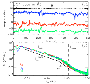
Figure 1.— Spectra of typical magnetic field components $B_{x}$, $B_{y}$ and $B_{z}$ measured by FGM from 04:10UT to 04:35UT on 29/02/2004. The vertical dashed lines denote the frequency range that k-filtering technique is applied. The spectral flattening above 2.4Hz is due to the FGM reaching the noise floor.

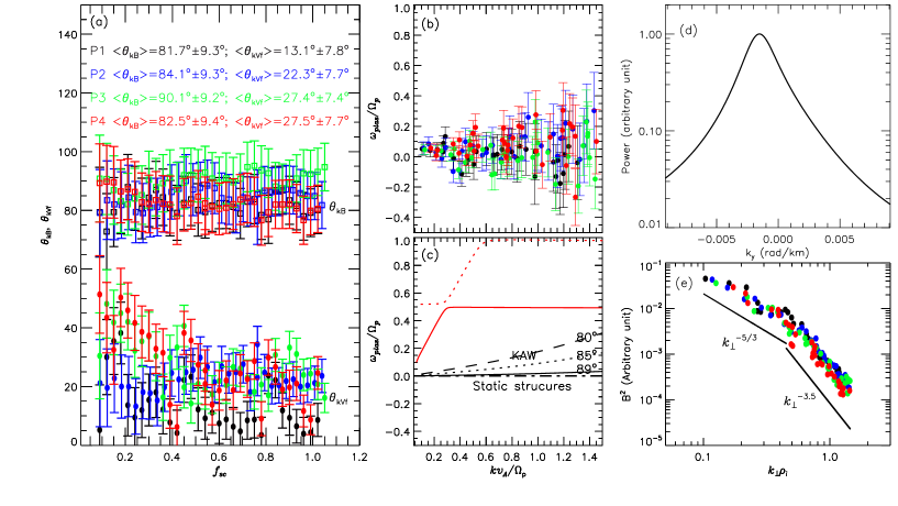
Figure 2.— (a) Angles $\theta_{\bf kB}$ (squares) and $\theta_{{\bf kV}_{f}}$ (solid dots) with related uncertainties computed by using the k-filtering technique during four time intervals. (b) Measured wave dispersion (filled dots), with estimated error bars. (c) The dispersion relation curves, computed from linear Vlasov theory, represent waves propagating at several observed angles $\theta_{\bf kB}$: black lines are kinetic Alfvén waves propagating at 80^∘ (dashed), 85^∘ (dotted) and 89^∘ (solid); the remaining red (solid and dotted) curves represent fast and Bernstein waves propagating at 89.5^∘. The proton angular gyrofrequency is $\Omega_{p}=2\pi f_{ci}$. The dot-dashed line represent static structures. (d)Power spectral density of magnetic field fluctuations as a function of $k_{y}$ at spacecraft-frame frequency 0.51Hz in P3. (e) The magnetic field $k_{\perp}$ spectra of all the four measured time intervals.

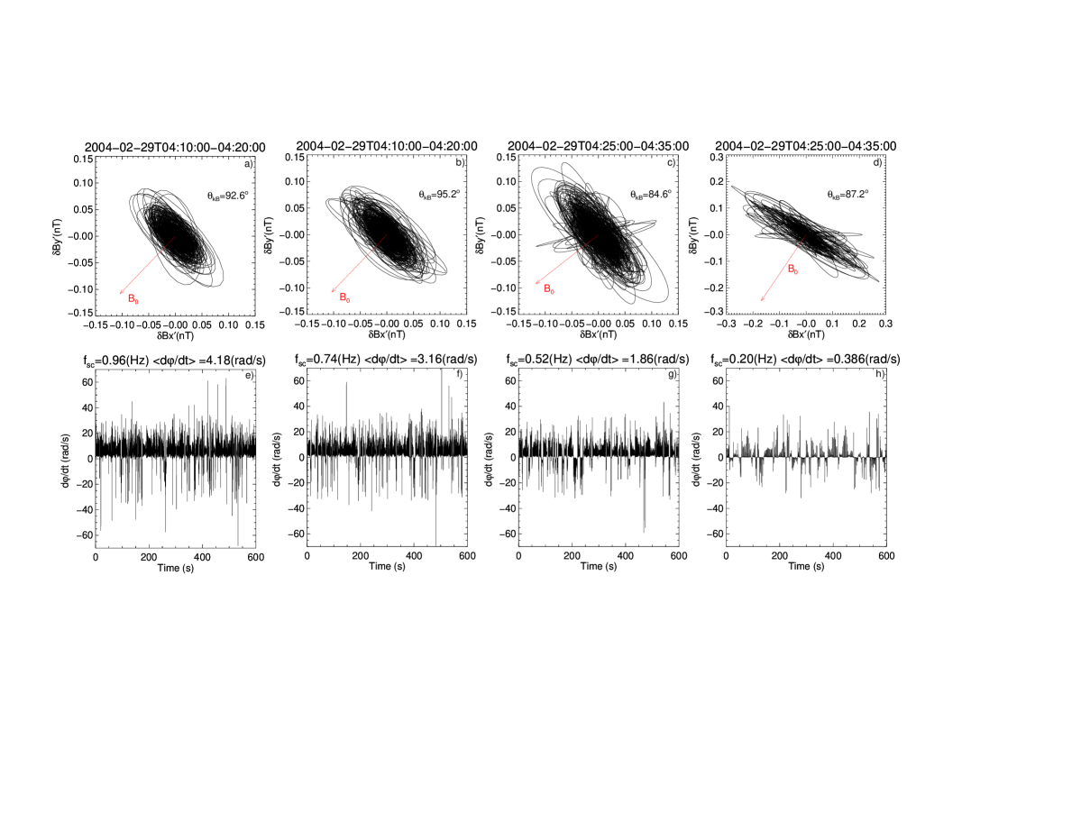
Figure 3.— Polarization analysis in the plane perpendicular to ${\bf k}$. Top panels: $\delta B_{x^{\prime}}-\delta B_{y^{\prime}}$ hodograph at frequencies (a) $f_{sc}=0.96$Hz, (b)0.74Hz in P3, and (c) 0.52Hz, (d) 0.2Hz in P4. The bottom panels display the corresponding polarizations at these frequencies. The wave propagation angle $\theta_{\bf kB}$ is a) 92.6^∘, b) 95.2^∘, c) 84.6^∘, and d) 87.2^∘. The mean values of $\langle d\varphi/dt\rangle$ are all positive. The wave frequencies in the solar wind frame determined by the k-filtering are all positive.

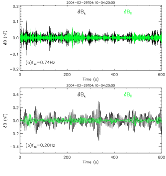
Figure 4.— Reconstructed time series of fluctuated magnetic field along wave vectors found by the k-filtering technique and along the background magnetic field ${\bf B}_{0}$ for the interval P3 at two spacecraft frequencies: (a) $f_{sc}=0.74$Hz, and (b) $f_{sc}=0.2$Hz. The data are taken from spacecraft C4.

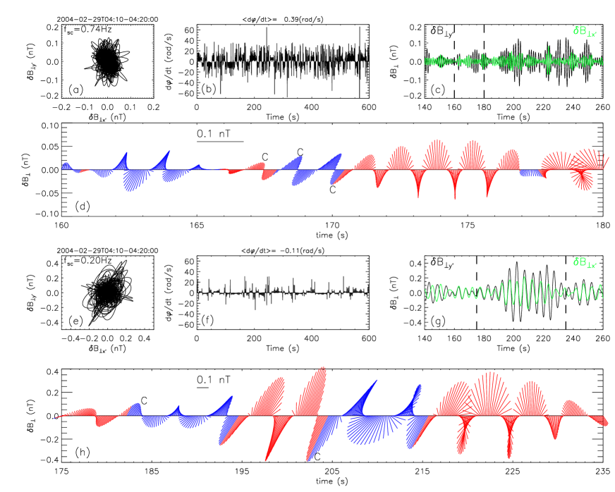
Figure 5.— Polarization analysis in the plane perpendicular to ${\bf B}_{0}$ at $f_{sc}=0.72$Hz (a,b,c,d) and 0.21Hz (e,f,g,h) for interval P3. (a) and (e): $\delta B_{\perp x^{\prime}}-\delta B_{\perp y^{\prime}}$ hodograph, (b) and (f): $d\varphi/dt$, (c) and (g): representative waveforms, magnetic field hodograms for the region between the two vertical lines are shown in (d) and (h). Blue and red denote right- and left-handed polarization. At the two frequencies, the wave vectors determined by k-filtering are $kv_{A}/\Omega_{0}$ =0.981 and 0.354. The data are taken from spacecraft C4.

References

- Alexandrova & Saur (2008) Alexandrova, O., & Saur, J. 2008, Geophys. Res. Lett., 35, 15102
- Alexandrova et al. (2006) Alexandrova, O., Mangeney, A., Maksimovic, M., et al. 2006, Journal of Geophysical Research (Space Physics), 111, 12208
- Alexandrova et al. (2009) Alexandrova, O., Saur, J., Lacombe, C., et al. 2009, Physical Review Letters, 103, 165003
- Alexandrova et al. (2012) Alexandrova, O., Lacombe, C., Mangeney, A., Grappin, R., & Maksimovic, M. 2012, ApJ, 760, 121
- Bale et al. (2005) Bale, S. D., Kellogg, P. J., Mozer, F. S., Horbury, T. S., & Reme, H. 2005, Physical Review Letters, 94, 215002
- Balogh et al. (2001) Balogh, A., et al. 2001, Ann. Geophys., 19, 1207 C1217.
- Bieber et al. (1996) Bieber, J.W., Wanner, W., Matthaeus, W.H. 1996, J. Geophys. Res., 101, 2511.
- Biskamp et al. (1996) Biskamp, D. et al. 1996, Phys. Rev. Lett. 76, 1264
- Bourouaine et al. (2012) Bourouaine, S., Alexandrova, O., Marsch, E., & Maksimovic, M. 2012, ApJ, 749, 102
- Chmyrev et al. (1988) Chmyrev, V. M., Bilichenko, S. V., Pokhotelov, V. I., Marchenko, V. A., & Lazarev, V. I. 1988, Phys. Scr, 38, 841
- Dasso et al. (2005) Dasso, S., Milano, L.J., Matthaeus, W.H., & Smith, C.W. 2005, ApJ, 635, L181.
- Eastwood et al. (2009) Eastwood, J.P., et al. 2009, Phys. Rev. Lett. 102, 035001.
- Gary (1999) Gary, S.P. 1999, J. Geophys. Res. 104, 6759.
- Gary & Smith (2009) Gary, S.P., & Smith, C.W. 2009, J. Geophys. Res., 114, A12105.
- Goldreich & Sridhar (1995) Goldreich, P., & Sridhar, S. 1995, ApJ, 438, 763.
- Grison et al. (2005) Grison, B., et al. 2005, Ann. Geophys. 23, 3699.
- He et al. (2012) He, J., Tu, C., Marsch, E., & Yao, S. 2012, ApJ, 745, L8
- Howes et al. (2008) Howes, G.G., et. al. 2008, Phys. Rev. Lett., 100, 065004.
- Howes & Quataert (2010) Howes, G.G., & Quataert, E. 2010, Astrophs. J., 709, L49.
- Horbury et al. (2005) Horbury, T. S., Forman, M.A., & Oughton, S. 2005, Plasma Phys. Controlled Fusion, 47, B703
- Huang et al. (2010) Huang, S.Y., et al. 2010, J. Geophys. Res., 115, A12211.
- Jian et al. (2006) Jian, L., Russell, C.T., Luhmann, J.G., & Skoug, R.M. 2006,Sol. Phys.239, 393.
- Johnstone et al. (1997) Johnstone, A. D., Alsop, C., Burge, S., et al. 1997, Space Sci. Rev., 79, 351
- Leamon et al. (1998) Leamon, R. J., Smith, C. W., Ness, N. F., Matthaeus, W. H., & Wong, H. K. 1998, J. Geophys. Res., 103, 47758.
- Li et al. (2001) Li, H., Gary, S.P., and Stawicki, O. 2001, Geophys. Res. Letts., 28, 1347.
- Li et al. (2010) Li, X., Lu, Q., Chen, Y., Li, B., & Xia, L. 2010, ApJ, 719, L190
- Marsch et al. (1982) Marsch, E., Schwenn, R., Rosenbauer, H., et al. 1982, J. Geophys. Res., 87, 52
- Matthaeus et al. (1990) Matthaeus, W. H., Goldstein, M. L., & Roberts, D. A. 1990, J. Geophys. Res., 95, 20,673.
- Narita et al. (2005) Narita, Y., et al. 2005, J. Geophys. Res. 110, A12 215.
- Narita et al. (2010) Narita, Y., Sahraoui, F., Goldstein, M. L., & Glassmeier, K.-H. 2010, Journal of Geophysical Research (Space Physics), 115, 4101
- Narita et al. (2011) Narita, Y., Gary, S.P., Saito, S., et al. 2011, Geophys. Res. Letts., 38, L05101.
- Onishchenko et al. (2008) Onishchenko, O. G., Krasnoselskikh, V. V., & Pokhotelov, O. A. 2008, Physics of Plasmas, 15, 022903
- Osmane et al. (2010) Osmane, A., Hamza, A. M., & Meziane, K. 2010, Journal of Geophysical Research (Space Physics), 115, 5101
- Pinçon & Motschmann (1998) Pinçon, J.-L., & Motschmann, U. 1998, ISSI Scientific Reports Series, 1, 65
- Perri et al. (2012) Perri, S., Goldstein, M. L., Dorelli, J. C., & Sahraoui, F. 2012, Physical Review Letters, 109, 191101
- Pinçon & Lefeuvre (1991) Pinçon, J.L., & Lefeuvre, F. 1991, J. Geophys. Res. 96, 178.
- Petviashvili & Pokhotelov (1992) Petviashvili, V., & Pokhotelov, O. 1992, Solitary waves in plasmas and in the atmosphere., Gordon and Breach, Philadelphia, PA (USA), 1992.
- Robert et al. (1998) Robert, P., Roux, A., Harvey, C.C., Dunlop, M.W., Daly, P.W., &. Glassmeier, K. H. 1998, Tetrahedron geometric factors, in Analysis Methods for Multi-Spacecraft Data, ISSI Sci. Rep., SR-001, pp. 323 C 348, Int. Space Sci. Inst., Bern.
- Reme et al. (2001) Reme, H., et al. 2001, Ann. Geophys.,19,1303.
- Sahraoui et al. (2004) Sahraoui, F. et al. 2004, Ann. Geophys. 22, 2283.
- Sahraoui et al. (2010a) Sahraoui, F., Goldstein, M.L., et al. 2010, Phys. Rev. Letts., 105, 131101.
- Sahraoui et al. (2010b) Sahraoui, F., et al. 2010, J. Geophys. Res., 115, A04206.
- Sahraoui et al. (2012) Sahraoui, F., Belmont, G., & Goldstein, M. L. 2012, ApJ, 748, 100
- Salem et al. (2012) Salem, C.S., Howes, G.G., et al. 2012, ApJL, 745, L9.
- Shebalin et al. (1983) Shebalin, J. V., Matthaeus, W. H., & Montgomery, D. 1983, Journal of Plasma Physics, 29, 525
- Schekochihin et al. (2009) Schekochihin, A. et al. 2009, Astrophys. J. Suppl. Ser. 182, 310.
- Smith et al. (2012) Smith, C.W., Vasques, B.J. & Hollweg, J.V. 2012, ApJ, 745, 8.
- Stawicki et al. (2001) Stawicki, O., Gary, S.P. and Li, H. 2001, J. Geophys. Res. 106, 8273.
- Sundkvist & Bale (2008) Sundkvist, D., & Bale, S. D. 2008, Physical Review Letters, 101, 065001
- Sundkvist et al. (2005) Sundkvist, D., Krasnoselskikh, V., Shukla, P. K., et al. 2005, Nature, 436, 825
- Taylor (1938) Taylor, G. I. 1938, Royal Society of London Proceedings Series A, 164, 476
- Tjulin et al. (2005) Tjulin, A., PinçOn, J.-L., Sahraoui, F., André, M., & Cornilleau-Wehrlin, N. 2005, Journal of Geophysical Research (Space Physics), 110, 11224
- Torrence & Compo (1998) Torrence, C., & Compo, G. P. 1998, Bulletin of the American Meteorological Society, 79, 61
- Verkhoglyadova et al. (2003) Verkhoglyadova, O. P., Dasgupta, B., & Tsurutani, B. T. 2003, Nonlinear Processes in Geophysics, 10, 335
- Volwerk et al. (1996) Volwerk, M., Louarn, P., Chust, T., et al. 1996, J. Geophys. Res., 101, 13335