Global tracking for an underactuated ships with bounded feedback controllers

Abstract

In this paper, we present a global state feedback tracking controller for underactuated surface marine vessels. This controller is based on saturated control inputs and, under an assumption on the reference trajectory, the closed-loop system is globally asymptotically stable (GAS). It has been designed using a 3 Degree of Freedom benchmark vessel model used in marine engineering. The main feature of our controller is the boundedness of the control inputs, which is an essential consideration in real life. In absence of velocity measurements, the controller works and remains stable with observers and can be used as an output feedback controller. Simulation results demonstrate the effectiveness of this method.

I Introduction

Precise tracking control of surface marine vessels (ships and boats) is often required in critical operations such as support around off-shore oil rigs [1]. This problem is of particular interest as marine vessels are often underactuated, i.e. the number of independent actuators is less than the degrees of freedom (DOF) to be controlled. In this paper, we consider the problem of tracking control of a 3-DOF vessel model (surge, sway and yaw [2]), working under two independent actuators capable of generating surge force and yaw moment only. It has been shown in [3, 4, 5] that under Brockett’s necessary condition [3], stabilization of this system is impossible with continuous or discontinuous time-invariant state feedback. This can be seen in [6] where the authors developed a continuous time-invariant controller that achieved global exponential position tracking but the vessel orientation could not be controlled. In addition, it is shown in [7] that the underactuated ship can not be transformed into a driftless chained system; which means that the control techniques used for the similar problem of nonholonomic mobile robot control cannot be applied directly to the underactuated ship control. Accordingly, control of underactuated vessels in this configuration has been studied rigorously by contemporary researchers, examples of which are [8, 9, 10, 11, 12].

In [7], the author showed that under discontinuous time-varying feedback, the underactuated vessel is strongly accessible and small-time locally controllable at any equilibrium. A discontinuous time-invariant controller was proposed which showed exponential convergence of the vessel towards a desired equilibrium point, under certain hypotheses imposed on the initial conditions. In [1], a continuous periodic time-varying feedback controller was presented that locally exponentially stabilizes the system on the desired equilibrium point by using a global coordinate transformation to render the vessel’s model homogenous. In [8], a combined integrator backstepping and averaging approach was used for tracking control, together with the continuous time-varying feedback controller for position and orientation control. This combined approach, later on used in [13], provides practical global exponential stability as the vessel converges to a neighborhoo d of the desired location or trajectory, the size of which can be chosen arbitrarily small. Jiang [14] used Lyapunov’s direct method for global tracking under the assumption that the reference yaw velocity requires persistent excitation condition; therefore implying that a straight line trajectory could not be tracked. This drawback was overcome in [15] and [16]. Do et al. [15] proposed a Lyapunov based method and backstepping technique for stabilization and tracking of underactuated vessel. In this work, conditions were imposed on the trajectory to transform the tracking problem into dynamic positioning, circular path tracking, straight line tracking and parking. Borhaug et al. have proposed a control scheme for straight line following of a formation of marine vessels in [17].

In this paper, we address the global tracking control of underactuated vehicles, using saturated state feedback control [18, 19, 20, 21, 22, 23]. Our work addresses the remaining case not treated in [15], i.e., the yaw angle of the tracked trajectory does not admit a limit at time goes to infinity. This research is therefore in the same direction as in [24], where the author achieved practical stability. Our algorithm provides asymptotic convergence to the tracked trajectory from any initial point. The advantage of using saturated controls is that the global asymptotic stability is ensured while the control inputs remain bounded, as real life actuators are all limited in output, see for instance [25], [26]. The proposed controller has been proven to work with state measurements, as well as with observers in the case where all states may not be measured (cf. also [25]).

The paper is organized as follows: the vessel model is presented in Section 2 and the control problem is formulated in Section 3. In Section 4, the controller is developed and the proof of stability is given. In Section 5, the stability of the controller is shown in presence of observation errors. Simulations are given in Section 6 and concluding remarks are presented in Section 7.

II Vessel Model

In this section, we discuss the physical model of the marine vessel and the related assumptions on physical phenomena associated with its motion. Then, a mathematical reformulation is presented, following variable and time-scale changes, to obtain a suitable form for control design.

II-A Physical Model

The general 6-DOF rigid body model for surface marine vessels presented in [2] can be reduced by considering surge, sway and yaw motions only, under the following assumptions [24],

$\displaystyle(H1)$

Heave, roll and pitch motions induced by drift forces of wind, wave and ocean current are neglected.

$\displaystyle(H2)$

The inertia, added mass and hydrodynamic damping matrices are diagonal.

The aft propeller configuration provides only the surge force $\displaystyle\tau_{u}$ and the yaw moment $\displaystyle\tau_{r}$. The kinematic and dynamic equations of the vessel can therefore be written as [15, 24]

$$\begin{array}[]{lcl}\left\{\begin{array}[]{lll}\dot{x}&=&u\cos\left(\psi\right)-v\sin\left(\psi\right),\quad\dot{y}=u\sin\left(\psi\right)+v\cos\left(\psi\right),\\ \dot{u}&=&\frac{1}{c}vr-au+\bar{\tau}_{1},\quad\dot{v}=-cur-bv,\\ \dot{\psi}&=&r,\quad\dot{r}=\kappa uv-dr+{\bar{\tau}_{2}},\end{array}\right.\end{array}$$ (1)

where $\displaystyle(x,y)$ and $\displaystyle\psi$ are the coordinates and the yaw angle of the vessel in the earth-fixed frame, and $\displaystyle u$, $\displaystyle v$ and $\displaystyle r$ denote the surge, sway and yaw velocities respectively. The control inputs $\displaystyle\bar{\tau}_{1}$ and $\displaystyle\bar{\tau}_{2}$ are the normalized expressions of the surge force and yaw moment, given as $\displaystyle\bar{\tau}_{1}=\frac{1}{m_{1}}{\tau_{u}}$ and $\displaystyle{\bar{\tau}_{2}}=\frac{1}{m_{3}}{\tau_{r}}$. The parameters $\displaystyle a$, $\displaystyle b$, $\displaystyle c$, $\displaystyle d$ and $\displaystyle\kappa$ are positive constants that represent the mechanical properties of the system, namely the inertia $\displaystyle m_{i}>0$ and hydrodynamic damping $\displaystyle d_{i}$, where $\displaystyle i=1,\ 2,\ 3$ corresponds to surge, sway and yaw motions respectively. The constants are defined as follows $\displaystyle a=\frac{d_{1}}{m_{1}}$, $\displaystyle b=\frac{d_{2}}{m_{2}}$, $\displaystyle c=\frac{m_{1}}{m_{2}}$, $\displaystyle d=\frac{d_{3}}{m_{3}}$, $\displaystyle\kappa=\frac{m_{1}-m_{2}}{m_{3}}$.

II-B Model for control

For control design, the system model (1) can be simplified by normalizing the physical parameters through straightforward variable and time-scale changes. For the sake of clarity, let us rewrite System (1) as follows,

$$\begin{array}[]{lcl}(\bar{S})\left\{\begin{array}[]{cll}{\left(\begin{array}[]{l}\dot{x}\\ \dot{y}\end{array}\right)}&=&{R_{\psi}}\left(\begin{array}[]{l}u\\ v\end{array}\right),\\ {\left(\begin{array}[]{l}\dot{u}\\ \dot{v}\end{array}\right)}&=&-D_{0}\left(\begin{array}[]{l}u\\ v\end{array}\right)-rA_{c}\left(\begin{array}[]{l}u\\ v\end{array}\right)+\left(\begin{array}[]{l}1\\ 0\end{array}\right){\bar{\tau}_{1}},\\ \dot{\psi}&=&r,\quad\dot{r}=\kappa uv-dr+\bar{\tau}_{2},\end{array}\right.\end{array}$$ (2)

where the matrices $\displaystyle D_{0}$, $\displaystyle R_{\psi}$ and $\displaystyle A_{c}$ are given as

$$\begin{array}[]{lcl}D_{0}=\left({\begin{array}[]{*{20}{c}}a&0\\ 0&b\end{array}}\right),\ {R_{\psi}}=\left({\begin{array}[]{*{20}{c}}{\cos\left(\psi\right)}&{-\sin\left(\psi\right)}\\ {\sin\left(\psi\right)}&{\cos\left(\psi\right)}\end{array}}\right),\ A_{c}=\left(\begin{array}[]{cc}0&{-1/c}\\ c&0\end{array}\right).\end{array}$$ (3)

Let us consider the following matrix $\displaystyle D_{\rho}=diag(\rho,c\rho)$, where $\displaystyle\rho$ is a positive constant to be chosen later. Then we obtain $\displaystyle A_{1}=D_{\rho}^{-1}A_{c}D_{\rho}$. The time scale $\displaystyle s:=dt$ is introduced in System (2) as well as the linear changes of variables $\displaystyle(u(t)/d\rho,v(t)/dc\rho)$ and $\displaystyle r(t)/d$, still denoted $\displaystyle(u(s),v(s)$ and $\displaystyle r(s)$ respectively.

After easy computations and by setting $\displaystyle\beta:=\frac{\kappa}{c\rho^{2}}$, $\displaystyle\tau_{1}:=\frac{\bar{\tau}_{1}}{\rho d^{2}}$, $\displaystyle\tau_{2}:=\frac{\bar{\tau}_{2}}{d^{2}}$ and $\displaystyle D=diag(a/d,b/d)$, the dynamics of the vessel, denoted by $\displaystyle(S)$, is rewritten as follows,

$$\begin{array}[]{lcl}(S)\left\{\begin{array}[]{cll}{\left(\begin{array}[]{l}\dot{x}\\ \dot{y}\end{array}\right)}&=&{R_{\psi}}D_{\rho}\left(\begin{array}[]{l}u\\ v\end{array}\right),\\ {\left(\begin{array}[]{l}\dot{u}\\ \dot{v}\end{array}\right)}&=&-D\left(\begin{array}[]{l}u\\ v\end{array}\right)-rA_{1}\left(\begin{array}[]{l}u\\ v\end{array}\right)+{\tau_{1}}\left(\begin{array}[]{l}1\\ 0\end{array}\right),\\ \dot{\psi}&=&r,\quad\dot{r}=\beta uv-r+\tau_{2}.\end{array}\right.\end{array}$$ (4)

III Problem Formulation

The goal of this paper is tracking control of the presented underactuated marine vessel by controlling its position and orientation. The vessel is forced to follow a reference trajectory which is generated by a “virtual vessel”, as follows [27, 28],

$$\begin{array}[]{lcl}(S_{re})\left\{\begin{array}[]{cll}{\left(\begin{array}[]{l}\dot{x}_{re}\\ \dot{y}_{re}\end{array}\right)}&=&R_{\psi_{re}}D_{\rho}\left(\begin{array}[]{l}u_{re}\\ v_{re}\end{array}\right),\\ {\left(\begin{array}[]{l}\dot{u}_{re}\\ \dot{v}_{re}\end{array}\right)}&=&-{D}\left(\begin{array}[]{l}u_{re}\\ v_{re}\end{array}\right)-r_{re}A_{1}\left(\begin{array}[]{l}u_{re}\\ v_{re}\end{array}\right)+\left(\begin{array}[]{l}1\\ 0\end{array}\right)\tau_{1,re},\\ \dot{\psi}_{re}&=&r_{re},\quad\dot{r}_{re}=\beta u_{re}v_{re}-r_{re}+\tau_{2,re},\end{array}\right.\end{array}$$ (5)

where all variables have similar meanings as in System (4). Tracking control is achieved by using saturated control inputs and under the assumption that the velocities are bounded [29, 30]. This assumption holds true physically as resistive drag forces increase as the velocity increases and therefore the latter cannot increase indefinitely if the control is bounded. These assumptions are also valid for the reference system and are formalized in the following manner:

Assumption 1.

There exist constraints on the control inputs and velocities such that

$$\begin{array}[]{lcl}\left|\bar{\tau}_{1}\right|\leq\bar{\tau}_{1,\max},\ \left|\bar{\tau}_{2}\right|\leq\bar{\tau}_{2,\max},\ \left|u\right|\leq\bar{u}_{\max},\ \left|v\right|\leq\bar{v}_{\max},\end{array}$$ (6)

where $\displaystyle\bar{\tau}_{1,\max}$, $\displaystyle\bar{\tau}_{2,\max}$, $\displaystyle\bar{u}_{\max}$ and $\displaystyle\bar{v}_{\max}$ are known positive constants. The velocities $\displaystyle u_{re}$, $\displaystyle v_{re}$ and the forces $\displaystyle\tau_{1,re}$ and $\displaystyle\tau_{2,re}$ verify the same bounds as above and the reference angle $\displaystyle\psi_{re}$ does not converge to a finite limit as $\displaystyle t$ tends towards infinity.

The variable and time-scale change defined in the previous section requires the following new bounds to be defined for the new control inputs $\displaystyle\tau_{1}$ and $\displaystyle\tau_{2}$, denoted by $\displaystyle\tau_{1,max}$ and $\displaystyle\tau_{2,max}$ respectively: $\displaystyle\tau_{1,max}=\frac{\bar{\tau}_{1,max}}{\rho d^{2}}$ and $\displaystyle\tau_{2,max}=\frac{\bar{\tau}_{2,max}}{d^{2}}$. We consider the following condition upon the saturation limits of the control inputs, to be used later on in the control design. We use here $\displaystyle m_{1}$ to denote $\displaystyle\min(a_{1}/2,b_{1})$.

$$\begin{array}[]{lcl}\text{{C1: }}\quad\beta\frac{\tau_{1,max}^{2}}{a_{1}m_{1}}<\tau_{2,max}.\end{array}$$ (7)

Note that this condition is always satisfied by choosing $\displaystyle\rho>\frac{\bar{\tau}_{1,max}}{d}\sqrt{\frac{\beta}{a_{1}m_{1}\bar{\tau}_{2,max}}}$. Our control objective is that $\displaystyle(S)$ follows $\displaystyle(S_{re})$. With respect to the frame of reference of the reference trajectory $\displaystyle(S_{re})$, the error system is defined as

$$\begin{array}[]{lcl}e_{x}=\cos(\psi_{re})(x-x_{re})+\sin(\psi_{re})(y-y_{re}),\quad e_{y}=-\sin(\psi_{re})(x-x_{re})+\cos(\psi_{re})(y-y_{re}),\\ e_{u}=u-u_{re},\ e_{v}=v-v_{re},\ e_{\psi}=\psi-\psi_{re},\ e_{r}=r-r_{re}.\end{array}$$ (8)

Defining new controllers $\displaystyle w_{1}$ and $\displaystyle\tilde{w}_{2}$, as follows, $\displaystyle w_{1}:=\tau_{1}-\tau_{1,re}$ and $\displaystyle\tilde{w}_{2}:=\tau_{2}-\tau_{2,re}$, the dynamics of system (8) becomes

$$\begin{array}[]{lcl}(S_{e})\left\{\begin{array}[]{cll}{\left(\begin{array}[]{l}\dot{e}_{x}\\ \dot{e}_{y}\end{array}\right)}&=&-r_{re}A_{1}\left(\begin{array}[]{l}e_{x}\\ e_{y}\end{array}\right)+D_{\rho}\left(\begin{array}[]{l}e_{u}\\ e_{v}\end{array}\right)+sin(e_{\psi})A_{1}D_{\rho}\left(\begin{array}[]{l}u_{re}\\ v_{re}\end{array}\right)\\ &&+\left(cos\left(e_{\psi}\right)-1\right)D_{\rho}\left(\begin{array}[]{l}u_{re}\\ v_{re}\end{array}\right)+\left(R_{e_{\psi}}-Id_{2}\right)\left(\begin{array}[]{l}e_{u}\\ e_{v}\end{array}\right),\\ {\left(\begin{array}[]{l}\dot{e}_{u}\\ \dot{e}_{v}\end{array}\right)}&=&-D\left(\begin{array}[]{l}e_{u}\\ e_{v}\end{array}\right)-r_{re}A_{1}\left(\begin{array}[]{l}e_{u}\\ e_{v}\end{array}\right)-e_{r}A_{1}\left(\begin{array}[]{l}u_{re}\\ v_{re}\end{array}\right)+\left(\begin{array}[]{l}1\\ 0\end{array}\right)w_{1}+e_{r}\left(\begin{array}[]{c}-e_{v}\\ e_{u}\end{array}\right),\\ \dot{e}_{\psi}&=&e_{r},\quad\dot{e}_{r}=\beta\left(uv-u_{re}v_{re}\right)-e_{r}+\tilde{w}_{2}.\end{array}\right.\end{array}$$ (9)

The control objective is to force the error system $\displaystyle(S_{e})$ to $\displaystyle 0$, using $\displaystyle w_{1}$ and $\displaystyle\tilde{w}_{2}$.

IV Controller design

We first develop the following intermediate result, concerning the bounds of $\displaystyle u$, $\displaystyle v$, $\displaystyle r$.

Lemma 1.

The variables $\displaystyle u$, $\displaystyle v$, $\displaystyle r$ are bounded and satisfy

$$\begin{array}[]{lcl}\begin{array}[]{cll}\mathop{\lim\sup}\limits_{t\to\infty}\|(u,v)\|&\leq&\frac{\tau_{1,\max}}{2\sqrt{a_{1}m_{1}}},\quad\mathop{\lim\sup}\limits_{t\to\infty}\left|r\right|\leq\tau_{2,\max}+\beta\frac{\tau_{1,\max}^{2}}{2a_{1}m_{1}}.\end{array}\end{array}$$ (10)

Proof.

Let us consider the positive definite function

$$\displaystyle V_{u,v}=\frac{1}{2}(u^{2}+v^{2}),$$

then

$$\displaystyle\dot{V}_{u,v}=u\dot{u}+v\dot{v} \displaystyle= \displaystyle u\left(-a_{1}u+rv+\tau_{1}\right)+v\left({-b_{1}v-ru}\right)$$

$$\displaystyle\leq \displaystyle-\frac{a_{1}}{2}u^{2}-b_{1}v^{2}+\frac{\tau_{1}^{2}}{2a_{1}}$$

$$\displaystyle\leq \displaystyle-m_{1}(u^{2}+v^{2})+\frac{\tau_{1}^{2}}{2a_{1}},$$

we can see that $\displaystyle\dot{V}_{u,v}\leq 0$ for $\displaystyle(u^{2}+v^{2})\geq\frac{\tau_{1}^{2}}{2a_{1}m_{1}}$, which directly implies the first inequality in (10) (see Chapter 9 of [31]). Similarly, consider $\displaystyle V_{r}=\frac{1}{2}r^{2}$ then, $\displaystyle\dot{V}_{r}=r\dot{r}=-r^{2}-r\left(\tau_{2}+\beta uv\right)=-r(r+\tau_{2}+\beta uv),$ $\displaystyle\dot{V}_{r}\leq 0$ for $\displaystyle|r|\geq|\tau_{2}|+|\beta uv|$, from which we derive the second inequality in (10). ∎

Remark 1.

As the reference trajectory system is similar to the vessel model, it can be shown that the limits defined in Lemma 1 are valid for $\displaystyle u_{re}$, $\displaystyle v_{re}$, $\displaystyle r_{re}$ as well.

We define a new control variable $\displaystyle w_{2}:=\beta\left(uv-u_{re}v_{ref}\right)+\tilde{w}_{2}$. As the upper bounds of $\displaystyle u$, $\displaystyle v$, $\displaystyle u_{re}$ and $\displaystyle v_{ref}$ are known according to Lemma 1 and Remark 1, we obtain

$$\begin{array}[]{lcl}\mathop{\lim\sup}\limits_{t\to\infty}\beta\left|uv-u_{re}v_{ref}\right|\leq\beta\frac{\tau_{1,max}^{2}}{a_{1}m_{1}}.\end{array}$$ (11)

If $\displaystyle|w_{2}|\leq U_{2}$, for a positive constant $\displaystyle U_{2}$, one must have $\displaystyle U_{2}+\beta\frac{\tau_{1,max}^{2}}{a_{1}m_{1}}\leq\tau_{2,max}$, which is guaranteed by Condition C1. With these preliminaries established, we will now proceed to fulfill the control objective by using the bounded controls $\displaystyle w_{1}$ and $\displaystyle w_{2}$. Let $\displaystyle\sigma(.)$ be a standard saturation function, i.e., $\displaystyle\sigma(t)=\frac{t}{\max(1,|t|)}$. The main result of the paper is given next.

Theorem 1.

If Assumption 1 and Condition C1 are fulfilled, then for an appropriate choice of constants $\displaystyle U_{1},\ \rho,\ \xi,\ M,\ U_{2},\ k_{1},\ k_{2},\ \mu$ satisfying:

$$\displaystyle a_{1}>U_{1}+\rho,\ U_{1}>\frac{\left|a_{1}-\frac{b_{1}}{c}\right|}{\min\left(a_{1},\ \frac{b_{1}}{c}\right)}\rho,\ U_{2}>0,$$

$$\displaystyle M>0,\ k_{1}>k_{2}-1>0,\ a_{1}+\xi=\mu\rho,\ b_{1}=\mu c\rho,$$

then the following controller ensures global asymptotic stability of the tracking error system $\displaystyle(S_{e})$:

$$\begin{array}[]{lcl}w_{1}&=&-U_{1}\sigma\left(\frac{\xi e_{u}}{U_{1}}\right)-\rho\sigma\left(M(e_{x}+\frac{1}{\mu}e_{u})\right),\\ w_{2}&=&-U_{2}\sigma\left(\frac{k_{1}}{U_{2}}e_{\psi}+\frac{k_{2}-1}{U_{2}}e_{r}\right).\end{array}$$ (12)

Proof of Theorem 1.

We first consider the errors $\displaystyle e_{\psi}$ and $\displaystyle e_{r}$ and take $\displaystyle k_{1},k_{2}>0$ large in the control input $\displaystyle w_{2}$ defined previously. The dynamics of $\displaystyle e_{\psi}$ and $\displaystyle e_{r}$ in $\displaystyle(S_{e})$ $\displaystyle\dot{e}_{\psi}=e_{r}$ and $\displaystyle\dot{e}_{r}=-e_{r}-U_{2}\sigma\left(\frac{k_{1}}{U_{2}}e_{\psi}+\frac{k_{2}-1}{U_{2}}e_{r}\right)$.

Lemma 2.

If $\displaystyle U_{2}>0$ and $\displaystyle k_{1}>k_{2}-1>0$, then after a sufficiently large time, the saturated control operates in its linear region and the errors $\displaystyle e_{\psi}$ and $\displaystyle e_{r}$ converge to zero exponentially.

Proof.

Let us consider the Lyapunov function $\displaystyle V$,

$$\begin{array}[]{lcl}V=\frac{\alpha}{2}e_{r}^{2}+S\left(\frac{k_{1}}{U_{2}}e_{\psi}+\frac{k_{2}-1}{U_{2}}e_{r}\right),\end{array}$$ (13)

where $\displaystyle S(\xi):=\int^{\xi}_{0}\sigma(s)ds$, and $\displaystyle\alpha=\frac{k_{1}-k_{2}+1}{U_{2}^{2}}>0$. Set $\displaystyle z:=\frac{k_{1}}{U_{2}}e_{\psi}+\frac{k_{2}-1}{U_{2}}e_{r}$. Then, one has

$$\begin{array}[]{lcl}\dot{V}=\alpha e_{r}\dot{e}_{r}+\sigma(z)\dot{z}=-\alpha e_{r}^{2}-(k_{2}-1)\sigma^{2}(z).\end{array}$$ (14)

Then $\displaystyle\dot{V}<0$ for $\displaystyle(e_{\psi},e_{r})\neq(0,0)$; and after a finite time we obtain $\displaystyle\left|\frac{k_{1}}{U_{2}}e_{\psi}+\frac{k_{2}-1}{U_{2}}e_{r}\right|\leq 1$. The dynamics of $\displaystyle e_{\psi}$ and $\displaystyle\ e_{r}$ becomes linear, i.e., $\displaystyle\dot{e}_{\psi}=e_{r}$ and $\displaystyle\dot{e}_{r}=-k_{1}e_{\psi}-k_{2}e_{r}$. As $\displaystyle k_{1},k_{2}>0$, $\displaystyle(e_{\psi},e_{r})$ converges exponentially to zero. ∎

Lemma 2 shows that the errors $\displaystyle e_{\psi}$ and $\displaystyle e_{r}$ converge to zero under the control $\displaystyle w_{2}$. We will now consider the errors $\displaystyle e_{u}$ and $\displaystyle e_{v}$. We choose the constants $\displaystyle\mu$ and $\displaystyle\xi$ such that $\displaystyle a_{1}+\xi=\mu\rho$ and $\displaystyle b_{1}=\mu c\rho$, implying that $\displaystyle\xi=b_{1}/c-a_{1}$ and $\displaystyle\mu>0$.

Lemma 3.

Consider the dynamics of $\displaystyle e_{u}$ and $\displaystyle e_{v}$ given in Equation (9). If $\displaystyle U_{1}$ and $\displaystyle\rho$ are chosen as $\displaystyle a_{1}>U_{1}+\rho$ and $\displaystyle U_{1}>\frac{\left|a_{1}-\frac{b_{1}}{c}\right|}{\min\left(a_{1},\frac{b_{1}}{c}\right)}\rho$, then the control $\displaystyle w_{1}:=-U_{1}\sigma\left(\frac{\xi e_{u}}{U_{1}}\right)-\rho\sigma_{1}(.)$, with $\displaystyle\sigma_{1}(.)$ to be chosen later, ensures that $\displaystyle e_{u}$ and $\displaystyle e_{v}$ satisfy the following inequalities:

$$\begin{array}[]{lcl}\mathop{\lim\sup}\limits_{t\to\infty}\|(e_{u},e_{v})\|\leqslant\frac{\rho}{\sqrt{m_{2}\tilde{a}}},\hbox{ with }\tilde{a}=\mathop{\inf}\limits_{t>0}\left(a_{1}+\xi\frac{\sigma\left(\frac{\xi e_{u}}{U_{1}}\right)}{\frac{\xi e_{u}}{U_{1}}}\right)>0,\quad m_{2}:=\min(\tilde{a}/2,b_{1}).\end{array}$$ (15)

Proof.

Notice that $\displaystyle\tilde{a}>0$ since it is trivially the case if $\displaystyle\xi\geq 0$, and otherwise, $\displaystyle\tilde{a}\geq a_{1}+\xi=\frac{b_{1}}{c}$. Then, one has $\displaystyle e_{u}\dot{e}_{u}+e_{v}\dot{e}_{v}=-a_{1}e_{u}^{2}-b_{1}e_{v}^{2}+e_{r}(e_{u}v_{re}-e_{v}u_{re})+e_{u}w_{1}$. By applying the control $\displaystyle w_{1}$, we get $\displaystyle e_{u}\dot{e}_{u}+e_{v}\dot{e}_{v}\leq-a_{1}e_{u}^{2}-b_{1}e_{v}^{2}-U_{1}e_{u}\sigma\left(\frac{\xi e_{u}}{U_{1}}\right)-\rho e_{u}\sigma_{1}(.)+C_{0}\left|e_{r}\right|\sqrt{e_{u}^{2}+e_{v}^{2}}$, where $\displaystyle C_{0}:=\bar{u}_{max}+\bar{v}_{max}$. According to Lemma 2, $\displaystyle e_{r}$ tends to zero, i.e., for large $\displaystyle t$, one has $\displaystyle e_{u}\dot{e}_{u}+e_{v}\dot{v}\leq-\left[a_{1}+\xi s(t)\right]e_{u}^{2}-b_{1}e_{v}^{2}-\rho e_{u}\sigma_{1}(.)$. Then (15) results from the following inequality

$$\begin{array}[]{lcl}e_{u}\dot{e}_{u}+e_{v}\dot{v}\leq-m_{2}(e_{u}^{2}+e_{v}^{2})+\frac{\rho^{2}\sigma_{1}^{2}(\cdot)}{\tilde{a}}.\end{array}$$ (16)

∎

Lemma 3 proves the convergence of $\displaystyle e_{u}$ and $\displaystyle e_{v}$ to a neighborhood of zero. Since $\displaystyle\tilde{a}\geq\min\left(a_{1},\frac{b_{1}}{c}\right)$, one gets that $\displaystyle\mathop{\lim\sup}\limits_{t\to\infty}\left|\frac{\xi e_{u}}{U_{1}}\right|<1$, and the controller exits saturation in finite time and enter its linear region of operation. We get $\displaystyle\sigma\left(\frac{\xi e_{u}}{U_{1}}\right)=\frac{\xi e_{u}}{U_{1}}$, and the dynamics of $\displaystyle e_{u}$ and $\displaystyle e_{v}$ become

$$\displaystyle\dot{e}_{u}=-\mu\rho e_{u}+r_{re}e_{v}-\rho\sigma_{1}(.)+e_{r}v_{re}-e_{r}e_{v},\quad\dot{e}_{v}=-\mu c\rho e_{v}-r_{re}e_{u}-e_{r}u_{re}+e_{r}e_{u}.$$

Define $\displaystyle W=\left(W_{1},W_{2}\right)^{T}:=(e_{x},e_{y})^{T}+(e_{u},e_{v})^{T}/\mu$. Then one has the following result.

Lemma 4.

Let $\displaystyle W$ defined previously and the controller $\displaystyle w_{1}$ given in (12) with $\displaystyle\sigma_{1}(.)=\sigma(MW_{1})$, where $\displaystyle M$ is an arbitrary positive constant. Then $\displaystyle W$ tends to a finite limit $\displaystyle\bar{W}=(0,\bar{W}_{2})^{T}$.

Proof.

The dynamics of $\displaystyle W$ can be expressed as

$$\displaystyle\dot{W} \displaystyle= \displaystyle-{r_{re}}{A_{1}}W+\frac{r_{re}}{\mu}{A_{1}}\left({\begin{array}[]{c}{e_{u}}\\ {e_{v}}\end{array}}\right)+\sin\left({{e_{\psi}}}\right){A_{1}}{D_{\rho}}\left({\begin{array}[]{c}{u_{re}}\\ {v_{re}}\end{array}}\right)+{D_{\rho}}\left({\begin{array}[]{{c}}{e_{u}}\\ {e_{v}}\end{array}}\right)+O\left({e_{\psi}^{2},\left|{e_{\psi}}\right|\left({\begin{array}[]{c}{e_{u}}\\ {e_{v}}\end{array}}\right)}\right)$$

$$\displaystyle-{D_{\rho}}\left({\begin{array}[]{c}{e_{u}}\\ {e_{v}}\end{array}}\right)-{r_{re}}\frac{A_{1}}{\mu}\left({\begin{array}[]{c}{e_{u}}\\ {e_{v}}\end{array}}\right)-\frac{{{\rho}}}{\mu}\sigma(MW_{1})\left({\begin{array}[]{{c}}1\\ 0\end{array}}\right)+O\left({\left|{e_{r}}\right|\left({1+\left\|(e_{u},e_{v})\right\|}\right)}\right).$$

In order to find the limsup of $\displaystyle\|W\|$, we calculate

$$\displaystyle{W^{T}}\dot{W} \displaystyle= \displaystyle\sin\left({{e_{\psi}}}\right){W^{T}}{A_{1}}{D_{\rho}}\left({\begin{array}[]{*{20}{c}}{{u_{re}}}\\ {{v_{re}}}\end{array}}\right)+{W^{T}}\left[{O\left({e_{\psi}^{2},\left|{{e_{\psi}}}\right|\left({\begin{array}[]{*{20}{c}}{{e_{u}}}\\ {{e_{v}}}\end{array}}\right)+O\left({\left|{{e_{r}}}\right|}\right)}\right)}\right]-\frac{{{\rho}}}{\mu}{W_{1}}\sigma(MW_{1}),$$

$$\displaystyle= \displaystyle O\left({\left\|W\right\|.\left\|{{e_{\psi}},{e_{r}}}\right\|}\right)-\frac{{{\rho}}}{\mu}{W_{1}}\sigma(MW_{1}),$$

which implies that $\displaystyle|W^{T}\dot{W}|+\frac{\rho}{\mu}W_{1}\sigma_{1}(MW_{1})\leqslant\|W\|O\left(\|e_{\psi},e_{r}\|\right)$. One deduces first that the time derivative of $\displaystyle\|W\|$ is integrable over $\displaystyle\mathbb{R}_{+}$ and thus $\displaystyle W$ admits a limit as $\displaystyle t$ tends to infinity. Therefore, the right-hand side of the previous inequality is integrable over $\displaystyle\mathbb{R}_{+}$ implying the same conclusion for $\displaystyle W_{1}\sigma(MW_{1})$. As both $\displaystyle W_{1}$ and $\displaystyle\dot{W}_{1}$ are bounded, then according to Barbalat’s Lemma, $\displaystyle W_{1}\rightarrow 0$ as $\displaystyle t\rightarrow\infty$. Consequently $\displaystyle W_{2}$ tends towards a finite value $\displaystyle\bar{W}_{2}$ as $\displaystyle t$ tends to infinity. ∎

Lemma 4 permits us to further improve the result of Lemma 3, as follows.

Lemma 5.

If Lemmas 3 and 4 hold true, then $\displaystyle e_{u}$ and $\displaystyle e_{v}$ converge to zero asymptotically.

Proof.

From Lemma 3 and setting $\displaystyle G(e_{u},e_{v}):=(e_{u}^{2}+e_{v}^{2})/2$, Equation (16) is rewritten as $\displaystyle\dot{G}+2m_{2}G\leq\frac{\rho^{2}\sigma_{1}^{2}(MW_{1})}{\tilde{a}}$. One concludes using Barbalat’s Lemma. ∎

So far, we have established that the errors $\displaystyle e_{\psi}$, $\displaystyle e_{r}$, $\displaystyle e_{u}$ and $\displaystyle e_{v}$ converge to zero. From Lemmas 4 and 5, we deduce that if $\displaystyle W_{1}\rightarrow 0$ and $\displaystyle e_{u}\rightarrow 0$, then $\displaystyle e_{x}$ will converge asymptotically to zero as well. We next address the convergence of the remaining error variable, $\displaystyle e_{y}$.

Lemma 6.

If Assumption 1 is satisfied, then $\displaystyle\bar{W}_{2}=0$ and $\displaystyle e_{y}$ converges asymptotically to zero.

Proof.

From Equation (IV) in Lemma 4, the dynamics of $\displaystyle W$ can be expressed as follows, $\displaystyle\dot{W}=-{r_{re}}{A_{1}}W+O\left({\left|{{e_{\psi}}}\right|,\left|{{e_{r}}}\right|,{W_{1}}\sigma\left({M{W_{1}}}\right)}\right)$. We define the new variable $\displaystyle\tilde{W}$ as follows, $\displaystyle\tilde{W}:=R_{\psi_{re}}W$, and the dynamics of $\displaystyle\tilde{W}$ is given by

$$\displaystyle\dot{\tilde{W}}={{\dot{\psi}}_{re}}{A_{1}}{R_{{\psi_{re}}}}W-{r_{re}}{R_{{\psi_{re}}}}{A_{1}}W+{R_{{\psi_{re}}}}O\left({\left|{{e_{\psi}}}\right|,\left|{{e_{r}}}\right|,{W_{1}}\sigma\left({M{W_{1}}}\right)}\right)=O\left({\left|{{e_{\psi}}}\right|,\left|{{e_{r}}}\right|,{W_{1}}\sigma\left({M{W_{1}}}\right)}\right).$$

Since $\displaystyle e_{\psi}$ and $\displaystyle e_{r}$ converge exponentially to zero and $\displaystyle W_{1}\sigma(MW_{1})$ is integrable over $\displaystyle\mathbb{R}_{+}$, then $\displaystyle\left\|\dot{\tilde{W}}\right\|$ is also integrable over $\displaystyle\mathbb{R}_{+}$, which means that $\displaystyle\tilde{W}$ converges to a finite limit $\displaystyle W^{l}$. Then, one gets that $\displaystyle-W_{2}\sin\left(\psi_{re}\right)$ and $\displaystyle W_{2}\cos\left(\psi_{re}\right)$ tend to $\displaystyle W^{l}_{1}$ and $\displaystyle W^{l}_{2}$ respectively, as $\displaystyle t$ tends to infinity. If $\displaystyle\bar{W}_{2}\neq 0$, then one easily shows that $\displaystyle\psi_{re}$ converges to a finite limit by considering whether $\displaystyle\left(W_{re}\right)_{2}=0$ or not. That contradicts Assumption 2 and $\displaystyle W$ must converge asymptotically to as well as $\displaystyle e_{y}$. ∎

It should be noted that the controller presented in Theorem 1 has been designed under the assumption that all state variables are known. In the next section, the study is extended to the case where only the position and orientation states of the vessel are available and the velocities need to be observed.

V Tracking without velocity measurement

In practical cases, only position and orientation feedbacks are available for navigation. Therefore the only available states of the vessel are $\displaystyle x,\ y,\ \psi$ along with the the complete coordinate state set of the virtual vessel to be followed. For such output feedback systems, the variables $\displaystyle u,v,r$ need to be observed. In this section, we will show that the controller presented in Theorem 1 is applicable in this case and the use of observation instead of measurement does not affect the stability. We suppose that the velocities are obtained through an observer such as that presented by Fossen and Strand in [32], or a robust differentiator such as that presented in [33]. In both cases, observation errors converge exponentially to zero. It can be noted that, when we use a differentiator, the estimated values $\displaystyle(\hat{u},\hat{v},\hat{r})$ of $\displaystyle(u,v,r)$, can be determined according to the following equation $\displaystyle(\hat{u},\hat{v})^{T}=D_{\rho}^{-1}R_{-\psi}(\hat{\dot{x}},\hat{\dot{y}})^{T}$ and $\displaystyle\hat{r}=\hat{\dot{\psi}}$, where $\displaystyle(\hat{\dot{x}},\hat{\dot{y}},\hat{\dot{\psi}})$ are the estimated values of $\displaystyle({\dot{x}},{\dot{y}},{\dot{\psi}})$ respectively.

Let us follow the same steps used in the demonstration of stability of system $\displaystyle(S_{e})$ with velocity measurement. The observation error related to the velocity are define as below: $\displaystyle f_{u}=u-\hat{u}$, $\displaystyle f_{v}=v-\hat{v}$ and $\displaystyle f_{r}=r-\hat{r}$. As the references are common, the observation errors can be described in terms of trajectory pursuit errors as $\displaystyle f_{u}=e_{u}-\hat{e}_{u}$, $\displaystyle f_{v}=e_{v}-\hat{e}_{v}$, and $\displaystyle f_{r}=e_{r}-\hat{e}_{r}$, where, $\displaystyle\hat{e}_{u}=\hat{u}-u_{re}$, $\displaystyle\hat{e}_{v}=\hat{v}-v_{re}$ and $\displaystyle\hat{e}_{r}=\hat{r}-r_{re}$. We note that the variable $\displaystyle x,y,\psi$ are measured and the related observation errors are null. The problem is transformed to demonstrate the stability of the error system $\displaystyle(S_{e})$ under control laws $\displaystyle w_{1}$ and $\displaystyle\tilde{w}_{2}$, which are now based on the observed values.
As in the previous case, we define $\displaystyle w_{2}:=\beta\left(\hat{u}\hat{v}-u_{re}v_{re}\right)+\tilde{w}_{2}$. Then the result of this section can be stated as the following theorem.

Theorem 2.

If Assumption 1 and Condition C1 are fulfilled, then for an appropriate choice of constants $\displaystyle U_{1},\ \rho,\ \xi,\ M,\ U_{2},\ k_{1},\ k_{2},\ \mu$, the following controller ensures global asymptotic stability of the tracking error system $\displaystyle(S_{e})$:

$$\begin{array}[]{lcl}w_{1}=-U_{1}\sigma\left(\frac{\xi\hat{e}_{u}}{U_{1}}\right)-\rho\sigma\left(M(e_{x}+\frac{1}{\mu}\hat{e}_{u})\right),w_{2}=-U_{2}\sigma\left(\frac{k_{1}}{U_{2}}e_{\psi}+\frac{k_{2}-1}{U_{2}}\hat{e}_{r}\right),\end{array}$$ (20)

if in addition the observer errors $\displaystyle f_{u}$, $\displaystyle f_{v}$ and $\displaystyle f_{r}$ converge asymptotically to zero and are integrable over $\displaystyle\mathbb{R}_{+}$ (i.e., the integrals of their norms over $\displaystyle\mathbb{R}_{+}$ are finite).

Remark 2.

The choice of constants $\displaystyle U_{1},\ \rho,\ \xi,\ M,\ U_{2},\ k_{1},\ k_{2},\ \mu$ remain the same as in the case of Theorem 1, therefore their expressions and conditions will not be repeated in this section.

Proof.

The proof of Theorem 2 is largely based upon the proof of Theorem 1, and is developed similarly. We first consider the dynamics of error variables $\displaystyle e_{\psi}$ and $\displaystyle e_{r}$:

$$\begin{array}[]{lcl}\dot{e}_{\psi}=e_{r},\quad\dot{e}_{r}=-e_{r}-U_{2}\sigma\left(\frac{k_{1}}{U_{2}}e_{\psi}+\frac{k_{2}-1}{U_{2}}e_{r}+f_{1}(t)\right)+f_{2}(t),\end{array}$$ (21)

where $\displaystyle f_{1}(t)=-\frac{k_{2}-1}{U_{2}}f_{r}$ and $\displaystyle f_{2}(t)=\beta(uv-\hat{u}\hat{v})$.

Lemma 7.

If $\displaystyle f_{1}(t)$ and $\displaystyle f_{2}(t)$ converge to zero asymptotically, then for some large positive constants $\displaystyle k_{1}$ and $\displaystyle k_{2}$, System (21) is globally asymptotically stable.

Proof.

Consider the Lyapunov function $\displaystyle V$ defined in (13). If $\displaystyle z:=\frac{k_{1}}{U_{2}}e_{\psi}+\frac{k_{2}-1}{U_{2}}e_{r}$, one gets

$$\begin{array}[]{lcl}\dot{V}&=&\alpha e_{r}\dot{e}_{r}+\sigma\left(\frac{k_{1}}{U_{2}}e_{\psi}+\frac{k_{2}-1}{U_{2}}e_{r}\right)\left[\frac{k_{1}}{U_{2}}\dot{e}_{\psi}+\frac{k_{2}-1}{U_{2}}\dot{e}_{r}\right],\\ &=&\alpha e_{r}\left(-e_{r}-U_{2}\sigma(z+f_{1})+f_{2}\right)+\sigma(z)\left[\frac{k_{1}}{U_{2}}e_{r}+\frac{k_{2}-1}{U_{2}}\left(-e_{r}-U_{2}\sigma(z+f_{1})+f_{2}\right)\right].\\ \end{array}$$ (22)

Using the inequality, $\displaystyle|ab|\leq\frac{a^{2}+b^{2}}{2}$, and taking $\displaystyle\alpha U_{2}=\frac{k_{1}-k_{2}+1}{U_{2}}>0$, we get

$$\displaystyle\dot{V} \displaystyle\leq \displaystyle-\frac{\alpha}{2}e_{r}^{2}-\left(k_{2}-1\right)\sigma\left(z\right)\sigma\left(z+f_{1}\right)+\alpha U_{2}e_{r}\left(\sigma\left(z\right)-\sigma\left(z+f_{1}\right)\right)+\frac{\alpha}{2}f_{2}^{2}+\frac{k_{2}-1}{U_{2}}\left|f_{2}\right|.$$

Using the inequalities $\displaystyle\left|\sigma\left(z\right)-\sigma\left(z+f_{1}\right)\right|\leq\left|f_{1}\right|$ and $\displaystyle\sigma\left(z\right)\sigma\left(z+f_{1}\right)\geq\sigma^{2}\left(z\right)-\left|f_{1}\right|$, one has

$$\dot{V}\leq-\frac{\alpha}{2}e_{r}^{2}-\left(k_{2}-1\right)\sigma^{2}\left(z\right)+\left(k_{2}-1\right)\left|f_{1}\right|+\alpha U_{2}\left|e_{r}\right|\left|f_{1}\right|+\frac{\alpha}{2}f_{2}^{2}+\frac{k_{2}-1}{U_{2}}\left|f_{2}\right|.$$

After a sufficiently large time interval $\displaystyle T$, it is assured that $\displaystyle|U_{2}f_{1}|<\frac{1}{6}$ $\displaystyle\forall t>T$, and

$$\begin{array}[]{lcl}\dot{V}&\leq&-\frac{\alpha}{3}e_{r}^{2}-(k_{2}-1)\sigma^{2}\left(z\right)+O\left(f_{1}^{2},\left|f_{2}\right|,f_{2}^{2}\right).\end{array}$$ (23)

From here, we obtain that $\displaystyle\mathop{\lim\sup}\limits_{t\to\infty}\left|e_{r}\right|=\mathop{\lim\sup}\limits_{t\to\infty}\left|\sigma(z)\right|=0$. ∎

Following the same steps as used in the previous section, we now demonstrate the convergence of the error variables ($\displaystyle e_{u}$,$\displaystyle e_{v}$,$\displaystyle e_{x}$,$\displaystyle e_{y}$) of System $\displaystyle(S_{e})$.

Lemma 8.

Consider the dynamics of $\displaystyle e_{u}$ and $\displaystyle e_{v}$ presented in Equation (9). Then, the control

$$\begin{array}[]{lcl}w_{1}=-U_{1}\sigma\left(\frac{\xi\hat{e}_{u}}{U_{1}}\right)-\rho\sigma_{1}(.)\end{array}$$ (24)

ensures that $\displaystyle e_{u}$ and $\displaystyle e_{v}$ are bounded and again verifiy the estimate (15).

Proof.

The argument exactly follows the line of the argument of Lemma 3 with the controller $\displaystyle w_{1}$ written as $\displaystyle w_{1}:=-U_{1}\sigma\left(\frac{\xi e_{u}}{U_{1}}+f\right)-\rho\sigma_{1}(.)$, where $\displaystyle f:=-\frac{\xi}{U_{1}}f_{u}$ converges to zero asymptotically and is integrable over $\displaystyle\mathbb{R}_{+}$, and by using the inequality $\displaystyle x\sigma(x+f)\geq x\sigma(x)-|x\sigma(f)|$. ∎

Similarly, the proof of convergence of $\displaystyle W_{1}$ to zero and $\displaystyle W_{2}$ to a finite limit, presented in Lemma 6, holds true and one concludes by showing that the limit of $\displaystyle W_{2}$ is zero as well. ∎

VI Simulations

The performance of the presented controller is illustrated by simulation. We apply the controller on an example of a monohull vessel, as considered in [15]. The length of this vessel is $\displaystyle 32$ m, and a mass of $\displaystyle 118\times 10^{3}$ kg. The parameters of the damping matrices as given as follow:

$$\begin{array}[]{lcl}\begin{array}[]{ccccccc}d_{1}&=&215\times 10^{2}Kgs^{-1},\quad d_{2}&=&97\times 10^{3}Kgs^{-1},\quad d_{3}&=&802\times 10^{4}Kgm^{2}s^{-1},\\ m_{1}&=&120\times 10^{3}Kg,\quad m_{2}&=&172.9\times 10^{3}Kg,\quad m_{3}&=&636\times 10^{5}Kgm^{2}.\\ \end{array}\end{array}$$ (25)

Based on these physical parameters, we find the parameters of System (1) as

$$\begin{array}[]{lcl}a=0.179,\ b=0.561,\ c=0.694,\ \beta=0.126,\kappa=8.32\times 10^{-4}.\end{array}$$ (26)

Then, the parameters of the controller and the normalized system $\displaystyle(S)$ are given by

$$\displaystyle a_{1}=1.421,\ b_{1}=4.449,\ d=0.126,\ k_{1}=10,\ k_{2}=10,\ U_{2}=0.1,\ U_{1}=\frac{a_{1}}{2},\ \rho=\frac{a_{1}}{4},\ M=0.1.$$

The reference trajectory is generated by considering the surge force and the yaw moment as constants $\displaystyle\tau_{1,re}=10$ and $\displaystyle\tau_{2,re}=0.05$ with the initial values

$$\displaystyle\left(x_{re}(0),y_{re}(0),\psi_{re}(0),u_{re}(0),v_{re}(0),r_{re}(0)\right)=\left(0\ m,0\ m,0\ rad,\ 0ms^{-1},0\ ms^{-1},0\ rads^{-1}\right)).$$

The initial conditions of the vessel are as follows:

$$\displaystyle\left(x(0),y_{re}(0),\psi(0),u(0),v(0),r(0)\right)=\left(50\ m,-150\ m,\frac{\pi}{4}\ rad,\ 50ms^{-1},0\ ms^{-1},0\ rads^{-1}\right).$$

The reference trajectory and the vessel are shown in a 2D coordinate plane in Figure 2.The vessel converges to the reference trajectory asymptotically and similarly for the position errors graph in Figure 2. The orientation error and its derivative also converge to zero, as seen in Figure 4. The convergence of $\displaystyle e_{u}$ and $\displaystyle e_{v}$ is shown in Figure 4. Figures 6 and 6 show the control signals $\displaystyle\tau_{1}$ and $\displaystyle\tau_{2}$ respectively and the controllers are clearly bounded. This is an essential property in real systems, where the control signals are constrained.

VII Conclusion

In this paper, we have addressed the problem of tracking of an underactuated surface vessel with only surge force an yaw moment. The proposed controller ensures global asymptotic tracking of the vessel, following a reference trajectory modeled by a virtual vessel. It is also shown that the stability of the system is not affected if the state measurements are replaced by observers. The using of saturated inputs is essential as in real life the actuators have limited output. Simulation results illustrate the performance of the controller.

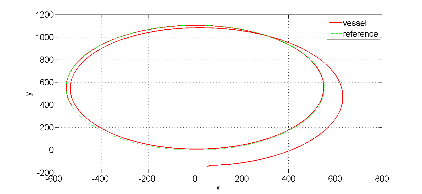
Figure 1: Reference trajectory and the vessel

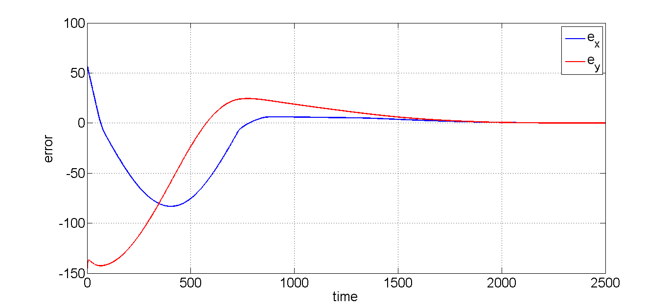
Figure 2: Errors $\displaystyle e_{x}$ and $\displaystyle e_{y}$

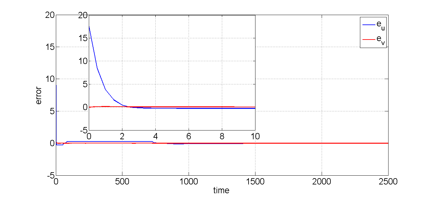
Figure 3: Errors $\displaystyle e_{u}$ and $\displaystyle e_{v}$

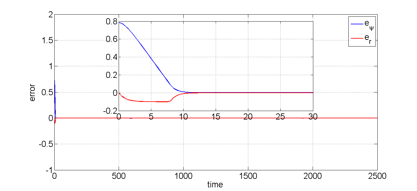
Figure 4: Errors $\displaystyle e_{\psi}$ and $\displaystyle e_{r}$

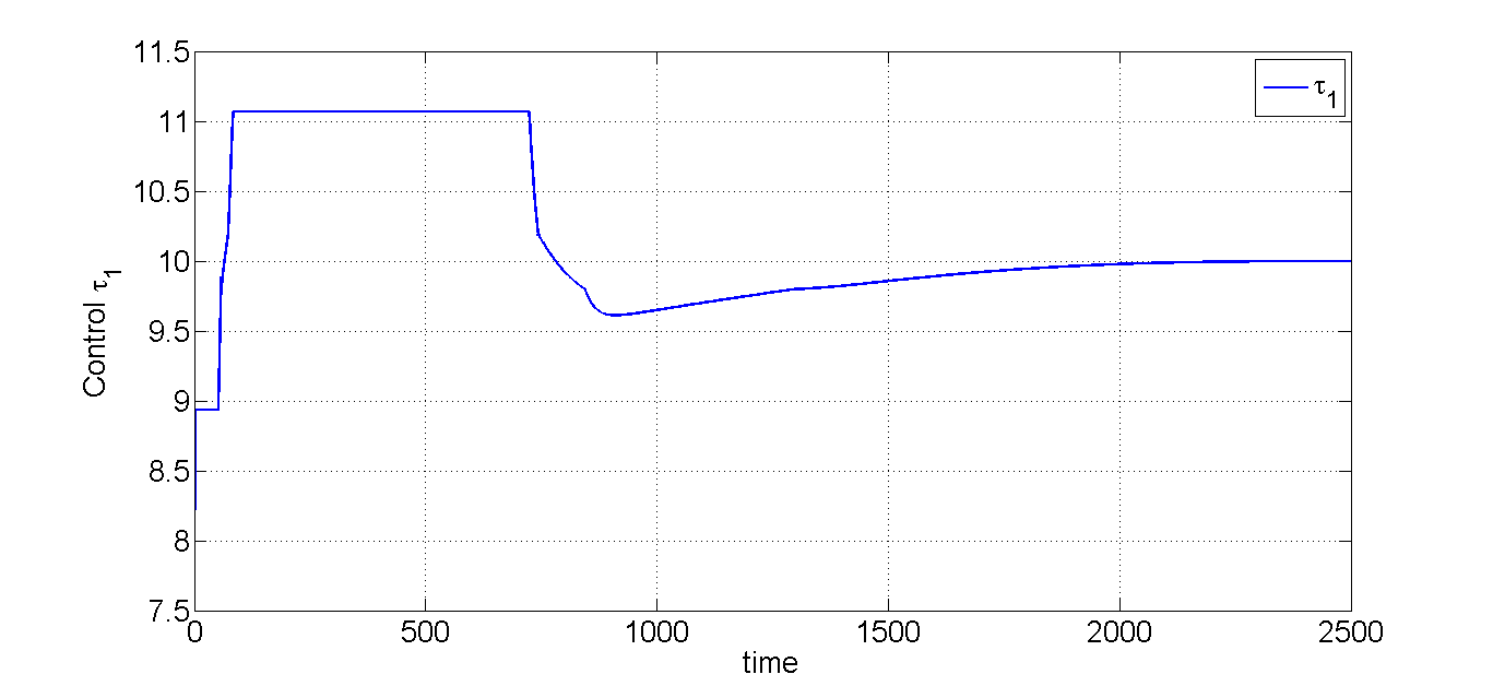
Figure 5: Control $\displaystyle\tau_{1}$

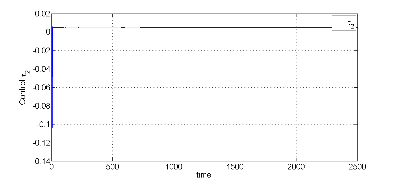
Figure 6: Control $\displaystyle\tau_{2}$

References

• [1] K.Y. Pettersen and O. Egeland. Exponential stabilization of an underactuated surface vessel. In the 35th IEEE Conference on Decision and Control, pages 967–972, Kobe, Japan, December 1996.
• [2] T.I. Fossen. Guidance and control of ocean vehicles. Wiley, New York, 1994.
• [3] R.W. Brockett. Asymptotic stability and feedback stabilization. In Differential Geometric Control Theory, pages 181–191. Birkhauser, Boston, 1983.
• [4] J.M. Coron and L. Rosier. A relation between continuous time-varying and discontinuous feedback stabilization. Journal of Mathematical Systems, Estimation and Control, 4(1):67–84, 1994.
• [5] J. Zabczyk. Some comments on stabilizability. Journal of Applied Mathematics and Optimization, 19:1–9, 1989.
• [6] J.M. Godhavn. Nonlinear tracking of underactuated surface vessels. In the 35th IEEE Conference on Decision and Control, pages 987–991, Kobe, Japan, December 1996.
• [7] M. Reyhanoglu. Control and stabilization of an underactuated surface vessel. In the 35th IEEE Conference on Decision and Control, pages 2371–2376, Kobe, Japan, December 1996.
• [8] K.Y. Pettersen and H. Nijmeijer. Global practical stabilization and tracking for an underactuated ship : a combined averaging and backstepping approach . Modeling, Identification and Control, 20(4):189–199, 1999.
• [9] T.I. Fossen, J.M. Godhavn, S.P. Berge, and K.P. Lindegaard. Nonlinear control of underactuated ships with forward speed compensation. In the IFAC NOLCOS’98, pages 121–127, Enschede, The Netherlands, July 1998.
• [10] S.P. Berge, K. Ohtsu, and T.I. Fossen. Nonlinear control of ships minimizing the position tracking errors. Modeling, Identification and Control, 20(3):177–187, 1999.
• [11] C. Samson. Control of Chained Systems Application on Path Following and Time-Varying Point-Stabilization of Mobile Robots. IEEE Transactions on Automatic Control, 40(1):64–77, 1995.
• [12] F. Bullo. Stabilization of relative equilibria for underactuated systems on Riemannian manifolds. Automatica, 36(12):1819–1834, 2000.
• [13] K.Y. Pettersen and H. Nijmeijer. Underactuated ship tracking control: Theory and experiments. International Journal of Control, 74(14):1435–1446, 2001.
• [14] Z. P. Jiang. Global tracking control of underactuated ships by lyapunov’s direct method. Automatica, 38:301–309, 2002.
• [15] K.D. Do, Z.P. Jiang, and J. Pan. Universal controllers for stabilization and tracking of underactuated ships. Systems and Control Letters, 47(4):299 – 317, 2002.
• [16] A. Behal, D. M. Dawson, W. E. Dixon, and Y. Fang. Tracking and regulation control of an underactuated surface vessel with nonintegrable dynamics. IEEE Transactions on Automatic Control, 47(3):495–500, 2002.
• [17] E. B rhaug, A. Pavlov, E. Panteley, and K.Y. Pettersen. Straight line path following for formations of underactuated marine surface vessels. Control Systems Technology, IEEE Transactions on, 19(3):493 –506, 2011.
• [18] Yacine Chitour, Wensheng Liu, and Eduardo Sontag. On the continuity and incremental-gain properties of certain saturated linear feedback loops. International Journal of Robust and Nonlinear Control, 5(5):413–440, 1995.
• [19] W. Liu, Y. Chitour, and E. Sontag. On finite-gain stabilizability of linear systems subject to input saturation. SIAM Journal on Control and Optimization, 34(4):1190–1219, 1996.
• [20] K. Yakoubi and Y. Chitour. Linear systems subject to input saturation and time delay: Finite-gain $\displaystyle l^{p}$-stabilization. SIAM Journal on Control and Optimization, 45(3):1084–1115, 2006.
• [21] K. Yakoubi and Y. Chitour. Linear systems subject to input saturation and time delay: Global asymptotic stabilization. Automatic Control, IEEE Transactions on, 52(5):874 –879, 2007.
• [22] Karim Yakoubi and Yacine Chitour. Stabilization and finite-gain stabilizability of delay linear systems subject to input saturation. In Applications of Time Delay Systems, volume 352 of Lecture Notes in Control and Information Sciences, pages 329–341. Springer Berlin Heidelberg, 2007.
• [23] Karim Yakoubi and Yacine Chitour. On the stabilization of linear discrete-time delay systems subject to input saturation. In Advanced strategies in control systems with input and output constraints, volume 352 of Lecture Notes in Control and Information Sciences, page 421 455. Springer Berlin Heidelberg, 2007.
• [24] D. Chwa. Global Tracking Control of Underactuated Ships With Input and Velocity Constraints Using Dynamic Surface Control Method. IEEE Transactions on Control Systems Technology, 19(6):1357–1370, 2011.
• [25] A. Gruszka, M. Malisoff, and F. Mazenc. Tracking control and robustness analysis for planar vertical takeoff and landing aircraft under bounded feedbacks. International Journal of Robust and Nonlinear Control, 2011. doi: 10.1002/rnc.1794.
• [26] A. Gruszka, M. Malisoff, and F. Mazenc. Bounded tracking controllers and robustness analysis for uavs. IEEE Transactions on Automatic Control, 2012. doi: 10.1109/TAC.2012.2203056.
• [27] L. Lapierre, D. Soetanto, and A. Pascoal. Nonlinear path following with applications to the control of autonomous underwater vehicles. In Decision and Control, 2003. Proceedings. 42nd IEEE Conference on, volume 2, pages 1256 – 1261 Vol.2, 2003.
• [28] M. Burger and K.Y. Pettersen. Smooth transitions between trajectory tracking and path following for single vehicles and formations. In 2nd IFAC Workshop on Distributed Estimation and Control in Networked Systems, (NecSys’10), 2010.
• [29] Y. Chitour. On the $\displaystyle l^{p}$-stabilization of the double integrator subject to input saturation. ESAIM Control, Optimisation and Calculus of Variations, 6:291–331, 2001.
• [30] S. Laghrouche, Y. Chitour, M. Harmouche, and F. Ahmed. Path following for a target point attached to a unicycle type vehicle. Acta Applicandae Mathematicae. doi: 10.1007/s10440-012-9672-8.
• [31] Hassan K. Khalil. Nonlinear Systems. Prentice-Hall. Inc., third edition, 2002.
• [32] T.U. Fossen and J.P. Strand. Passive nonlinear observer design for ships using lyapunov methods: full-scale experiments with a supply vessel. Automatica, 35(1):3 – 16, 1999.
• [33] Y. Chitour. On Time-Varying High-Gain Observers for Numerical Differentiation. IEEE Transactions on Automatic Control, 47(9):1565–1569, 2002.