The matrix sign function for solving surface wave problems in homogeneous and laterally periodic elastic half-spaces

Dedicated to Vladimir I. Alshits on the occasion of his 70th anniversary.

Keywords: surface waves, anisotropy, half-space

Abstract

The matrix sign function is shown to provide a simple and direct method to derive some fundamental results in the theory of surface waves in anisotropic materials. It is used to establish a shortcut to the basic formulas of the Barnett-Lothe integral formalism and to obtain an explicit solution of the algebraic matrix Riccati equation for the surface impedance. The matrix sign function allows the Barnett-Lothe formalism to be readily generalized for the problem of finding the surface wave speed in a periodically inhomogeneous half-space with material properties that are independent of depth. No partial wave solutions need to be found; the surface wave dispersion equation is formulated instead in terms of blocks of the matrix sign function of $i$ times the Stroh matrix.

1 Introduction

The theory of surface waves in homogeneous anisotropic elastic half-spaces has enjoyed remarkable progress in the 1960’s and 1970’s. The general framework developed by Stroh [1] for solving static and dynamic elasticity problems has proved to be very fruitful for study of surface waves. In a series of classic papers, e.g. [2, 3], Barnett and Lothe employed the framework of Stroh to develop an elegant integral matrix formalism that underpins existence and uniqueness considerations for surface waves and that allows one to determine the surface wave speed without having to solve for any partial wave solutions. The Barnett-Lothe integral formalism was quickly realized to serve as a corner stone for the surface wave theory. On this basis, Chadwick and Smith [4] provided a thorough exposition of the complete theory for surface waves in anisotropic elastic solids, summarizing the major developments up to that time, 1977. Later on, a significant contribution came from Alshits. With his co-workers, he has done much work on extending the formalism of Stroh, Barnett and Lothe to various problems of crystal acoustics, see the bibliography in this Special Issue. A full historical record and a broad overview of the surface wave related phenomena may be found in [5, 6].

The purpose of this paper is both to present a fresh perspective on the integral formalism for surface waves and also to provide new results, including a generalization to laterally periodic half-spaces. The central theme is the use of the matrix sign function which allows a quick derivation and a clear interpretation of the integral formalism of [2]. The application of the matrix sign function in the context of the Stroh formulation of elastodynamics was apparently first noted by [7] in the course of calculation of impedance functions for a solid cylinder. We reconsider the classical surface wave problem in terms of the matrix sign function, showing in the process that it provides a natural solution procedure. For instance, it is known that the surface impedance matrix $\mathbf{Z}$ satisfies an algebraic Riccati equation [8], but it has not been used to directly solve for $\mathbf{Z}$. Here we give the first explicit solution of this Riccati equation for the impedance. Another important attribute of the matrix sign function is that it allows the Barnett-Lothe formalism to be readily generalized to finding the surface wave speed in a periodically inhomogeneous half-space whose material properties are independent of depth (i.e. a 2D laterally periodic half-space). For this case, the present results provide a procedure that circumvents the need for partial wave solutions. Instead it establishes the dispersion equation in terms of the matrix sign function which can be evaluated by one of the optional methods, in particular in the integral form similar to the Barnett-Lothe representation of the homogeneous case.

The outline of the paper is as follows. The surface wave problem is defined in §2 in terms of the Stroh matrix $\mathbf{N}$. The matrix sign function $\operatorname{sign}i\mathbf{N}$ is introduced and discussed in §3 where it is shown to supply a novel and possibly advantageous route to the Barnett-Lothe integral formalism. An explicit solution of the algebraic Riccati equation for the surface impedance matrix $\mathbf{Z}$ is derived in §4. Application of the matrix sign function to formulating and solving the surface wave dispersion equation in a laterally periodic half-space is considered in §5, with the numerical examples given for a bimaterial configuration. The Appendix highlights explicit links between the sign function and some related matrix functions.

2 Background and problem definition

The equations of equilibrium for time harmonic motion (with the common factor $\mathrm{e}^{-i\omega t}$ everywhere omitted but understood) are

$$\partial_{j}\sigma_{ij}=-\rho\omega^{2}u_{i},\quad\sigma_{ij}=c_{ijkl}\partial_{l}u_{k}\ \ (i,j,k,l=1,2,3),$$ (1)

where $\rho$ is mass density, $c_{ijkl}$ are the elements of the elastic tensor $\mathbf{C}$ referred to an orthonormal coordinate system, $u_{i}$ and $\sigma_{ij}$ are elements of the displacement $\mathbf{u}({\mathbf{x}},t)$ and stress $\boldsymbol{\sigma}({\mathbf{x}},t)$. We first consider a uniform elastic half-space $\mathbf{n}\cdot\mathbf{x}\geq 0$, ($|\mathbf{n}|=1$) with constant density and elastic moduli. Solutions are sought in the form of surface waves propagating in the direction $\mathbf{m}$ parallel to the free surface ($\mathbf{m}\cdot\mathbf{n}=0$, $|\mathbf{m}|=1$):

$$\begin{pmatrix}\mathbf{u}\\ \mathbf{n}\boldsymbol{\sigma}\end{pmatrix}=\begin{pmatrix}\mathbf{a}(\mathbf{n}\!\cdot\!\mathbf{x})\\ -ik\mathbf{l}(\mathbf{n}\cdot\mathbf{x})\end{pmatrix}\,\mathrm{e}^{ik\mathbf{m}\cdot\mathbf{x}}.$$ (2)

The equations of equilibrium (1) take the form of a differential equation for the 6-vector $\boldsymbol{\eta}$ [3],

$$\frac{\mathrm{d}\boldsymbol{\eta}}{\mathrm{d}y} =ik\mathbf{N}\boldsymbol{\eta},\quad\text{with}\ \ \boldsymbol{\eta}(y)=\begin{pmatrix}\mathbf{a}(y)\\ \mathbf{l}(y)\end{pmatrix},$$ (3)

$$\mathbf{N} =-\begin{pmatrix}(nn)^{-1}(nm)&(nn)^{-1}\\ (mn)(nn)^{-1}(nm)-(mm)+\rho v^{2}\mathbf{I}&(mn)(nn)^{-1}\end{pmatrix},$$ (4)

where $v=\omega/k$, the 3$\times$3 matrix $\left(pq\right)$ has components $(pq)_{jk}=p_{i}c_{ijkl}q_{l}$ for arbitrary vectors $\mathbf{p}$ and $\mathbf{q}$, and $\mathbf{I}$ is the identity matrix. The real-valued Stroh matrix $\mathbf{N}$ satisfies $\mathbf{N}^{T}=\mathbf{K}\mathbf{N}\mathbf{K}$ where ^T indicates transpose and $\mathbf{K}$ in block matrix form comprises zero blocks on the diagonal and identity blocks off the diagonal. Denote the eigenvalues and eigenvectors of $i\mathbf{N}$ by $\lambda_{\alpha}$ and $\boldsymbol{\xi}_{\alpha}=\left(\mathbf{a}_{\alpha},\mathbf{l}_{\alpha}\right)^{T}$ ($\alpha=1,...,6$), and introduce the matrix $\mathbf{\Gamma}=\left\|\boldsymbol{\xi}_{1},...,\boldsymbol{\xi}_{6}\right\|$ with columns $\boldsymbol{\xi}_{\alpha}.$ Assume in the following the normal situation where all $\lambda_{\alpha}$ are distinct. Then the above symmetry of $\mathbf{N}$ yields the orthogonality/completeness relations in the form [2, eqs. 2.8-2.12]

$$\mathbf{\Gamma}^{T}\mathbf{K\mathbf{\Gamma}}=\mathbf{I}\quad\Leftrightarrow\quad\mathbf{\Gamma}\mathbf{K}\mathbf{\Gamma}^{T}=\mathbf{I},$$ (5)

where the normalization $\boldsymbol{\xi}_{\alpha}^{T}{\mathbf{K}}\boldsymbol{\xi}_{\alpha}=1$ has been adopted. Hereafter we use the same notation $\mathbf{I}$ for the identity matrix regardless of its algebraic dimension.

Throughout this paper we restrict our interest to the subsonic surface waves and thus assume that $v$ is less than the so-called limiting wave speed $\hat{v}$, see [3, 4, 6]. This implies that $i\lambda_{\alpha}$ are all nonzero and in pairs of complex conjugates (denoted below by ^∗), so the set of eigenvalues and eigenvectors of $i\mathbf{N}$ can be split into a pair of triplets as

$$\lambda_{\alpha}=-\lambda_{\alpha+3}^{\ast}\quad(\mathrm{Re}\lambda_{\alpha}<0)\quad\Rightarrow\quad\boldsymbol{\xi}_{\alpha}^{\ast}=\boldsymbol{\xi}_{\alpha+3},\quad\alpha=1,2,3.$$ (6)

These two triplets are commonly referred to as physical $(\alpha=1,2,3)$ and nonphysical $(\alpha=4,5,6)$ since they define partial modes that, respectively, decay or grow with increasing $\mathbf{n}\cdot\mathbf{x}$. The eigenvector matrix $\mathbf{\Gamma}$ partitioned according to (6) is written in the block form as

$$\mathbf{\Gamma}=\begin{pmatrix}\mathbf{A}_{1}&\mathbf{A}_{2}\\ \mathbf{L}_{1}&\mathbf{L}_{2}\end{pmatrix}\ \ \text{with}\ \ \begin{aligned} \mathbf{A}_{1}&=\left\|\mathbf{a}_{1},\mathbf{a}_{2},\mathbf{a}_{3}\right\|,\ \ \mathbf{A}_{2}=\left\|\mathbf{a}_{4},\mathbf{a}_{5},\mathbf{a}_{6}\right\|=\mathbf{A}_{1}^{*},\\ \mathbf{L}_{1}&=\left\|\mathbf{l}_{1},\mathbf{l}_{2},\mathbf{l}_{3}\right\|,\ \ \ \ \,\mathbf{L}_{2}=\left\|\mathbf{l}_{4},\mathbf{l}_{5},\mathbf{l}_{6}\right\|=\mathbf{L}_{1}^{*},\end{aligned}$$ (7)

where the blocks $\mathbf{A}_{1}$, $\mathbf{L}_{1}$ and $\mathbf{A}_{2}$, $\mathbf{L}_{2}$ describe the physical and nonphysical (decaying and growing) wave solutions, respectively. From (6) $\mathbf{\Gamma}^{\ast}=\mathbf{\Gamma K}$ and so the orthogonality/completeness relations (5) may be cast in the subsonic domain to the form

$$\mathbf{\Gamma}^{+}\mathbf{K\mathbf{\Gamma}}=\mathbf{K}\quad\Leftrightarrow\quad\mathbf{\Gamma}\mathbf{K\mathbf{\Gamma}}^{+}=\mathbf{K},$$ (8)

where ⁺ denotes the Hermitian transpose. Note that the relations (8) admit interpretation in terms of the energy flux into the depth.

The surface wave solution comprises the decaying solutions only and therefore must have the form

$$\mathbf{a}(y)=\mathbf{A}_{1}\,\mathrm{e}^{y{\boldsymbol{\lambda}}}\,\mathbf{v},\quad\mathbf{l}(y)=\mathbf{L}_{1}\,\mathrm{e}^{y{\boldsymbol{\lambda}}}\,\mathbf{v}\ \ \text{with }\ {\boldsymbol{\lambda}}=\mathrm{diag}(\lambda_{1},\lambda_{2},\lambda_{3}),$$ (9)

where $\mathbf{v}$ is some fixed vector. The surface wave problem for the homogeneous medium is posed as finding for a given wavenumber $k\in\mathbb{R}^{+}$ the surface wave speed $v=v_{s}\in\mathbb{R}$ for which the surface traction $\mathbf{l}(0)$ vanishes, and hence $\mathbf{v}$ is a null vector of $\mathbf{L}_{1}$ (although this is not a fruitful avenue to follow, which is the whole point of the Barnett-Lothe solution procedure based on the integral representation).

A variety of related notations have been used for the surface wave problem. We generally follow Barnett and Lothe [9] where the notation is based upon that of [3]. Barnett and Lothe [9] also provide comparisons of their notation with that used by Chadwick and Smith [4], which is closer to that of Ting [5]. The slight notational differences are related to the choice of the $6-$vector in (3), and amounts to different signs for the diagonal or off-diagonal elements of the $6\times 6$ matrix analogous to $\mathbf{N}$.

3 The matrix sign function $\operatorname{sign}i\mathbf{N}$

3.1 Definition

The sign function of a matrix $\mathbf{M}$ is conveniently defined by analogy with the scalar definition as [10]

$$\operatorname{sign}\mathbf{M}=\mathbf{M}\,\big{(}\mathbf{M}^{2}\big{)}^{-1/2},$$ (10)

where the principle branch of the square root function with branch cut on the negative real axis is understood; $z=(z^{2})^{1/2}\,\operatorname{sign}z$ with $\operatorname{sign}z=+1(-1)$ if $\mathrm{Re}z>0(<0)$. As a result, the sign function of a matrix $\mathbf{M}$ with eigenvalues and eigenvectors denoted by $\lambda_{\alpha}$ and $\boldsymbol{\xi}_{\alpha}$ satisfies

$$\mathbf{M}\boldsymbol{\xi}_{\alpha}=\lambda_{\alpha}\boldsymbol{\xi}_{\alpha}\quad\Rightarrow\quad\big{(}\operatorname{sign}\mathbf{M}\big{)}\boldsymbol{\xi}_{\alpha}=\pm\boldsymbol{\xi}_{\alpha}\ \mathrm{for}\ \lambda_{\alpha}\in\mathbb{C}^{\pm}.$$ (11)

Note that $\operatorname{sign}\mathbf{M}$ is unchanged under $\mathbf{M}\rightarrow a\mathbf{M}+ib\mathbf{I}$, $a\in\mathbb{R}^{+},\,b\in\mathbb{R}$, and it is undefined for eigenvalues lying on the imaginary axis ($\mathrm{Re}\lambda_{\alpha}=0$). We also note for later use the property $\operatorname{sign}\big{(}\mathbf{U}\mathbf{M}\mathbf{U}^{-1}\big{)}=\mathbf{U}\big{(}\operatorname{sign}\mathbf{M}\big{)}\mathbf{U}^{-1}$. Evaluation of the matrix sign function is possible with a variety of numerical methods [11], the simplest being Newton iteration of $\mathbf{M}_{k+1}=\frac{1}{2}(\mathbf{M}_{k}+\mathbf{M}_{k}^{-1})$, $\mathbf{M}_{0}=\mathbf{M}$, with $\mathbf{M}_{k}\rightarrow\operatorname{sign}\mathbf{M}$ in the limit as $k\rightarrow\infty$, although this can display convergence problems. Schur decomposition, which does not require matrix inversion, is very stable, and is readily available, e.g. [12]. The function $\operatorname{sign}\mathbf{M}$ also has integral representations, which we will use in order to shed fresh light on the integral formalism in the surface wave theory. See [13, 11] for reviews of the matrix sign function.

The following expression for the matrix sign function is based on (10) combined with an integral representation for the matrix square root function [14, 11]

$$\operatorname{sign}\mathbf{M}=\frac{2}{\pi}\mathbf{M}\int_{0}^{\infty}\mathrm{d}t\,\big{(}t^{2}\mathbf{I}+\mathbf{M}^{2}\big{)}^{-1}.$$ (12)

Equation (12) may be converted into the following form using a change of integration variable

$$\operatorname{sign}\mathbf{M}=\left\langle\mathbf{M}_{\theta}\right\rangle\ \ \text{with }\ \ \mathbf{M}_{\theta}\equiv(\cos\theta\mathbf{I}-i\sin\theta\mathbf{M})^{-1}(\cos\theta\mathbf{M}-i\sin\theta\mathbf{I}),$$ (13)

where

$$\langle\cdot\rangle=\frac{1}{\pi}\int_{0}^{\pi}\cdot\,\mathrm{d}\theta$$

denotes the average. Differentiation of $\mathbf{M}_{\theta}$ yields

$$\frac{\mathrm{d}\mathbf{M}_{\theta}}{\mathrm{d}\theta}=i\big{(}\mathbf{M}_{\theta}^{2}-\mathbf{I}\big{)},$$ (14)

which implies $\langle\mathrm{e}^{i\phi\mathbf{M}_{\theta}}\rangle=\langle\mathrm{e}^{-i\phi\mathbf{M}_{\theta}}\rangle^{-1}=\cos\phi\mathbf{I}+i\sin\phi\langle\mathbf{M}_{\theta}\rangle$ for any $\phi$. This provides alternative identities for the matrix sign function, such as

$$\operatorname{sign}\mathbf{M}=\big{\langle}\frac{\sin(\phi\mathbf{M}_{\theta})}{\sin\phi}\big{\rangle}=\big{\langle}\frac{\mathbf{M}_{\theta}\cos(\phi\mathbf{M}_{\theta})}{\cos\phi}\big{\rangle},$$ (15)

where the value of $\phi$ is arbitrary as long as the denominator, $\sin\phi$ or $\cos\phi$, does not vanish. The special case of eq. (13)₁ corresponds to the limit as $\phi\rightarrow 0$ in (15).

3.2 $\operatorname{sign}i\mathbf{N}$ and the Barnett-Lothe matrices

Let us apply the above definition and properties of the matrix sign function to the case $\operatorname{sign}i\mathbf{N}$ where $\mathbf{N}$ is the Stroh matrix given in (4) and considered in the subsonic domain $v<\hat{v}$. The eigenspectrum of $\mathbf{N}$ is assumed partitioned according to (6). Hence equation (11)₂ taken with $\mathbf{M}=i\mathbf{N}$ reads

$$\left(\operatorname{sign}i\mathbf{N}\right)\boldsymbol{\xi}_{\alpha}=-\boldsymbol{\xi}_{\alpha},\ \left(\operatorname{sign}i\mathbf{N}\right)\boldsymbol{\xi}_{\alpha+3}=\boldsymbol{\xi}_{\alpha+3},\ \alpha=1,2,3,$$ (16)

Denote the blocks of $\operatorname{sign}i\mathbf{N\ }$($=\mathbf{K}\left(\operatorname{sign}i\mathbf{N}\right)^{T}\mathbf{K}$) as

$$\operatorname{sign}i\mathbf{N}=i\begin{pmatrix}\mathbf{S}&\mathbf{Q}\\ \mathbf{B}&\mathbf{S}^{T}\end{pmatrix}\ \mathrm{with}\ \mathbf{Q=Q}^{T},\ \mathbf{B=B}^{T},\ \text{tr}\,\mathbf{S}=0,$$ (17)

where $\mathbf{S,\ Q,\ B}$ are all real since so is $\mathbf{N}$. Note that $\operatorname{sign}i\mathbf{N}$ and hence $\mathbf{S}$ are traceless. Appearance of the Barnett-Lothe notations on the right-hand side will become clear in the course of the upcoming derivation. The involutory property of the matrix sign function, $\big{(}\operatorname{sign}i\mathbf{N}\big{)}^{2}=\mathbf{I}$, implies the identities

$$\mathbf{BS}+\mathbf{S}^{T}\mathbf{B}=\mathbf{0},\ \ \mathbf{SQ}+\mathbf{QS}^{T}=\mathbf{0},\ \ \mathbf{S}^{2}+\mathbf{QB}=-\mathbf{I}.$$ (18)

Taking into account the spectral representation $i\mathbf{N}=\mathbf{\Gamma}\mathrm{diag}(\boldsymbol{\lambda},-\boldsymbol{\lambda}^{\ast})\mathbf{\Gamma}^{-1}$ and the relation (5)₂ yields the spectral decomposition of the matrix $\operatorname{sign}i\mathbf{N}$ in the form

$$\operatorname{sign}i\mathbf{N} =\mathbf{\Gamma}\mathrm{diag}(-\mathbf{I},\mathbf{I})\mathbf{\Gamma}^{T}\mathbf{K}=\begin{pmatrix}\mathbf{A}_{2}\mathbf{L}_{2}^{T}-\mathbf{A}_{1}\mathbf{L}_{1}^{T}&\mathbf{A}_{2}\mathbf{A}_{2}^{T}-\mathbf{A}_{1}\mathbf{A}_{1}^{T}\\ \mathbf{L}_{2}\mathbf{L}_{2}^{T}-\mathbf{L}_{1}\mathbf{L}_{1}^{T}&\mathbf{L}_{2}\mathbf{A}_{2}^{T}-\mathbf{L}_{1}\mathbf{A}_{1}^{T}\end{pmatrix}$$ (19)

$$=\mathbf{I}-2\begin{pmatrix}\mathbf{A}_{1}\mathbf{L}_{1}^{T}&\mathbf{A}_{1}\mathbf{A}_{1}^{T}\\ \mathbf{L}_{1}\mathbf{L}_{1}^{T}&\mathbf{L}_{1}\mathbf{A}_{1}^{T}\end{pmatrix}=\mathbf{I}-2\begin{pmatrix}\mathbf{A}_{1}\\ \mathbf{L}_{1}\end{pmatrix}\begin{pmatrix}\mathbf{A}_{1}\\ \mathbf{L}_{1}\end{pmatrix}^{T}\mathbf{K\ }\left(=\mathbf{I}-2\mathbf{P}_{-}\right),\mathbf{\ \ }$$

where we have noted the projector $\mathbf{P}_{-}$ on physical modes: $\mathbf{P}_{-}\mathbf{\Gamma=\Gamma}$$\begin{pmatrix}\mathbf{I}&\mathbf{0}\\ \mathbf{0}&\mathbf{0}\end{pmatrix}$ (see more in Appendix). From (17) and (19),

$$\mathbf{S}=i(2\mathbf{A}_{1}\mathbf{L}_{1}^{T}-\mathbf{I}),\ \mathbf{Q}=2i\mathbf{A}_{1}\mathbf{A}_{1}^{T},\quad\mathbf{B}=2i\mathbf{L}_{1}\mathbf{L}_{1}^{T}.$$ (20)

Assume that $\mathbf{A}_{1}$ and hence $\mathbf{Q}$ are invertible (we will return to this point later). Introduce the surface impedance $\mathbf{Z}=i\mathbf{L}_{1}\mathbf{A}_{1}^{-1}$. It is Hermitian due to (8)${}_{1}.$ Plugging (17) into (16)₁ gives $\mathbf{SA}_{1}+\mathbf{QL}_{1}=i\mathbf{A}_{1}$ which, with regard for the invertibility of $\mathbf{Q}$, enables expressing $\mathbf{Z}$ through the blocks of $\operatorname{sign}i{\mathbf{N.}}$ Thus

$$\mathbf{Z}=i\mathbf{L}_{1}\mathbf{A}_{1}^{-1}\left(=\mathbf{Z}^{+}\right)\ \Leftrightarrow\ \mathbf{Z}=-\mathbf{Q}^{-1}(\mathbf{I}+i\mathbf{S})~{}.$$ (21)

Note from (21) that, for any $v,$ $\det\mathbf{S}=0$ (since $\mathbf{Q}^{-1}\mathbf{S}$ is antisymmetric, see also (18)₂) and that $\det\left(\mathbf{I}+i\mathbf{S}\right)$ is real (since $\mathbf{Z=Z}^{+}$).

General significance of $\operatorname{sign}i\mathbf{N}$ for surface waves is immediate when one considers the boundary condition which demands that a non-zero surface displacement exerts zero surface traction. Since a surface wave is composed of decaying modes only, this means there must exist a vector $\mathbf{v}\neq 0$ such that

$$\left(\operatorname{sign}i{\mathbf{N}}\right)\begin{pmatrix}\mathbf{v}\\ \mathbf{0}\end{pmatrix}=\begin{pmatrix}-\mathbf{v}\\ \mathbf{0}\end{pmatrix}\quad\Rightarrow\quad\left\{\begin{aligned} ({\mathbf{I}}+i{\mathbf{S}}){\bf v}&=0,\\ {\mathbf{B}}{\bf v}&=0.\end{aligned}\right.$$ (22)

Hence both $\det\mathbf{B}$ and $\det\left(\mathbf{I}+i\mathbf{S}\right)$ must vanish at the surface wave speed $v=v_{s}$. For the case in hand of a uniform material, these are not two independent conditions but one condition. Indeed, the traction-free boundary condition can be posed in the form $\det\mathbf{L}_{1}=0,$ hence from (20) and (21)₁ determinants of $\mathbf{B,}$ of $\mathbf{I}+i\mathbf{S~{}}\left(=2\mathbf{A}_{2}\mathbf{L}_{1}^{+}\right)$ and of $\mathbf{Z}$ vanish simultaneously. Note that the equation $\det\left(\mathbf{I}+i\mathbf{S}\right)=0$ reduces to $\mathrm{tr}\left({\mathbf{S}}^{2}\right)=-2$ (since $\mathrm{tr}\mathbf{S}=0$ and $\det\mathbf{S}=0$). Also at $v=v_{s},$ the common null vector $\mathbf{v}$ of $\mathbf{I}+i\mathbf{S}$ and $\mathbf{B}$ can be cast as $\mathbf{v}=\mathbf{a}+i\mathbf{b}$ with linear independent real vectors $\mathbf{a}$ and $\mathbf{b,}$ hence $\mathbf{B}$ is rank one. To summarize, the subsonic surface wave speed $v=v_{s}$ can be determined from $\det\mathbf{L}_{1}=0$ or else from any of the equivalent real dispersion equations (see [5, eqs. (12.10-1)-(12.10-4)])

$$\det\mathbf{Z}=0\ \Leftrightarrow\mathrm{tr}\left({\mathbf{S}}^{2}\right)=-2\ \Leftrightarrow\det{\mathbf{B}}=0\ \ \left(\Rightarrow{(\mathrm{tr}{\mathbf{B}})^{2}=\mathrm{tr}({\mathbf{B}}^{2})}\right),$$ (23)

which all are expressed through the blocks of the matrix $\operatorname{sign}i{\mathbf{N}}$.

Equations (18), (20), (21), (23) are basic relations of the Barnett-Lothe formalism with regard to surface wave theory. Interestingly, we have arrived at these relations by single means of the definition of sign function of $i$ times the Stroh matrix $\mathbf{N}=\mathbf{K}\mathbf{N}^{T}\mathbf{K}$, without specifying the method of this function evaluation and without explicitly attending to the fundamental elasticity tensor which underlies development of Barnett-Lothe formalism in [2, 3, 4]. It is instructive to highlight an explicit link between the two lines of derivation, see next.

3.3 Linking $\operatorname{sign}i\mathbf{N}$ to the fundamental elasticity tensor $\mathbf{N}_{\theta}$

Following [2, 3, 4], introduce the so-called [4] fundamental elasticity tensor

$$\mathbf{N}_{\theta}=-\begin{pmatrix}[\![ss]\!]^{-1}[\![sr]\!]&[\![ss]\!]^{-1}\\[0.0pt] [\![rs]\!][\![ss]\!]^{-1}\![\![sr]\!]-[\![rr]\!]&[\![rs]\!][\![ss]\!]^{-1}\end{pmatrix}$$ (24)

$$\mathrm{where}\ [\![pq]\!]=\left(pq\right)-\left[\mathbf{m\cdot p}\right]\left[\mathbf{m\cdot q}\right]\rho v^{2}\mathbf{I\ \ }\mathrm{with}\ \mathbf{p,q}=\mathbf{r},\mathbf{s}:$$

$$\qquad\qquad\mathbf{r}=\cos\theta\mathbf{m}+\sin\mathbf{n},\ \mathbf{s=-}\sin\theta\mathbf{m+}\cos\theta\mathbf{n.}$$

The matrix $\mathbf{N}_{\theta}$ is defined in the subsonic domain which means that $v$ is small enough to guarantee existence of $[\![ss]\!]^{-1}$ for any $\theta$. Note that $\mathbf{N}_{\theta}$ at $\theta=0$ is equal to the Stroh matrix $\mathbf{N}$ defined in (4).

Lemma 1

The matrix sign function of $i$ times the Stroh matrix $\mathbf{N}$ is $i$ times the angular average of the fundamental elasticity tensor $\mathbf{N}_{\theta}$

$$\operatorname{sign}i\mathbf{N}=i\langle\mathbf{N}_{\theta}\rangle\ \Rightarrow\ \begin{array}[]{c}\mathbf{S}=-\left\langle[\![ss]\!]^{-1}[\![sr]\!]\right\rangle,\ \mathbf{Q}=-\left\langle[\![ss]\!]^{-1}\right\rangle\\ \mathbf{B}=\left\langle[\![rr]\!]-[\![rs]\!][\![ss]\!]^{-1}[\![sr]\!]\right\rangle.\end{array}$$ (25)

Proof: Equation (13) with $\mathbf{M}\equiv i\mathbf{N}$ reads

$$\operatorname{sign}i\mathbf{N}=i\langle\mathbf{G}\rangle\quad\text{with}\ \ \mathbf{G}\equiv(\cos\theta\mathbf{I}+\sin\theta\mathbf{N})^{-1}(\cos\theta\mathbf{N}-\sin\theta\mathbf{I}).$$ (26)

Let us show that $\mathbf{N}_{\theta}$ defined in (24) and $\mathbf{G}$ given by (26)₂ are one and the same. Substitution into $\mathbf{G}$ the representation [4, eq. (3.15)]

$$\mathbf{N}=(\mathbf{X}-\mathbf{Y})^{-1}\mathbf{J}(\mathbf{X}+\mathbf{Y})\ \ \text{where}\ \ \mathbf{J}=\begin{pmatrix}\mathbf{0}&\mathbf{I}\\ -\mathbf{I}&\mathbf{0}\end{pmatrix},$$ (27)

$$\mathbf{X}-\mathbf{Y}=\begin{pmatrix}(nn)&{\bf 0}\\ (mn)&-\mathbf{I}\end{pmatrix},\ \ \mathbf{X}+\mathbf{Y}=\begin{pmatrix}[\![mm]\!]&{\bf 0}\\ -(nm)&-\mathbf{I}\end{pmatrix},$$

yields, using $\mathrm{e}^{\mathbf{J}\theta}=\cos\theta\mathbf{I}+\sin\theta\mathbf{J}$,

$$\mathbf{G}= \big{(}\cos\theta(\mathbf{X}-\mathbf{Y})+\sin\theta\mathbf{J}(\mathbf{X}+\mathbf{Y})\big{)}^{-1}\big{(}\cos\theta\mathbf{J}(\mathbf{X}+\mathbf{Y})-\sin\theta(\mathbf{X}-\mathbf{Y})\big{)}$$

$$= \big{(}\mathrm{e}^{\mathbf{J}\theta}\mathbf{X}-\mathrm{e}^{-\mathbf{J}\theta}\mathbf{Y}\big{)}^{-1}\mathbf{J}\big{(}\mathrm{e}^{\mathbf{J}\theta}\mathbf{X}+\mathrm{e}^{-\mathbf{J}\theta}\mathbf{Y}\big{)}$$

$$= \big{(}\mathbf{X}-\mathrm{e}^{-2\mathbf{J}\theta}\mathbf{Y}\big{)}^{-1}\mathbf{J}\big{(}\mathbf{X}+\mathrm{e}^{-2\mathbf{J}\theta}\mathbf{Y}\big{)}.$$ (28)

Noting the identities

$$\mathbf{X}-\mathrm{e}^{-2\mathbf{J}\theta}\mathbf{Y}=\begin{pmatrix}[\![ss]\!]&\mathbf{0}\\[0.0pt] \![\![rs]\!]&-\mathbf{I}\end{pmatrix},\ \ \mathbf{X}+\mathrm{e}^{-2\mathbf{J}\theta}\mathbf{Y}=\begin{pmatrix}[\![rr]\!]&\mathbf{0}\\ -[\![sr]\!]&-\mathbf{I}\end{pmatrix},$$ (29)

it follows that

$$\mathbf{G}=\begin{pmatrix}[\![ss]\!]&\mathbf{0}\\[0.0pt] \![\![rs]\!]&-\mathbf{I}\end{pmatrix}^{-1}\begin{pmatrix}\mathbf{0}&\mathbf{I}\\ -\mathbf{I}&\mathbf{0}\end{pmatrix}\begin{pmatrix}[\![rr]\!]&\mathbf{0}\\ -[\![sr]\!]&-\mathbf{I}\end{pmatrix}=\mathbf{N}_{\theta}.$$ (30)

Combining (30) with (26)₁ completes the proof of (25). $\blacksquare$

Note that by the definition of $\mathbf{G}$ in (26) the eigenvectors of $\mathbf{N}_{\theta}(=\mathbf{G})$ are independent of $\theta$ and that eq. (14) with $\mathbf{M}_{\theta}\equiv i\mathbf{\mathbf{N}}_{\theta}$ reads

$$\frac{\mathrm{d}\mathbf{N}_{\theta}}{\mathrm{d}\theta}=-\mathbf{I}-\mathbf{N}_{\theta}^{2}.$$ (31)

Thus we have used the defining properties of sign function of the Stroh matrix $\mathbf{N}$ to obtain the basic relations (18), (20), (21), (23) of the Barnett-Lothe integral formalism, and then we made appear the fundamental elasticity matrix $\mathbf{N}_{\theta}$ but only in the context of one of possible (integral) representations of the sign function. This is different from the original methodology of [2, 3, 4] which follows a somewhat inverse line of derivation. It proceeds from $\mathbf{N}_{\theta}$ and establishes its properties such as (31) which are then used to arrive at the relations (18), (20), (21), (23). One way or another, the core is that the surface wave speed $v=v_{s}$ can be defined through the matrix sign function which admits evaluation by different integral formulas, e.g. eqs. (12), (15), (67) and (69), or iteration schemes, or otherwise. Interestingly, some of these ’indirect’ methods for calculating $\langle\mathbf{N}_{\theta}\rangle$ have been discussed in the literature, though with no mention of the matrix sign function. For instance, Gundersen and Lothe [15] propose a scheme tantamount to Newton iteration, while Condat and Kirchner [16] describe a method based on continued fractions that appears to be similar to a stable algorithm for computing the matrix sign function [17].

In conclusion, a remark is in order concerning invertibility of $\mathbf{Q}$ in the subsonic domain $v<\widehat{v}$. By definition of the latter, the eigenvalues $\mathbf{N}$ for $v<\widehat{v}$ cannot lie on the real axis, so $\mathbf{G}$ in (26)₂ is well-defined and hence, due to $\mathbf{G=N}_{\theta},$ the matrix $[[ss]]$ in (24) is non-singular. Since $[[ss]]$ is obviously positive definite at $v=0,$ it follows that $[[ss]]$ is positive within the whole subsonic domain $v<\widehat{v}$ (this of itself is an alternative definition of the subsonic domain). Using $\mathbf{Q=-}\left\langle[[ss]]^{-1}\right\rangle$ as given in (25) shows that $\mathbf{Q}$ is indeed invertible in the subsonic domain which implies that $\mathbf{A}_{1,2}$ are invertible and $\mathbf{Z}$ exists at any $v<\widehat{v}$. Note that we did not employ the fundamental elasticity tensor $\mathbf{N}_{\theta}$ in this proof.

4 The surface impedance as defined by Riccati equation

The surface impedance matrix $\mathbf{Z,}$ which is introduced in the subsonic domain by any of the following relations

$$\mathbf{l}_{\alpha}=-i\mathbf{Z}\mathbf{a}_{\alpha}\ \ \left(\alpha=1,2,3\right)\quad\Leftrightarrow\quad\mathbf{l}\left(y\right)=-i\mathbf{Z}\mathbf{a}\left(y\right)\quad\Leftrightarrow\quad\mathbf{Z}=i\mathbf{L}_{1}\mathbf{A}_{1}^{-1},$$ (32)

plays a central role in the theory of surface waves. It is a crucial ingredient in surface-wave uniqueness and existence considerations [3, 9] and is of fundamental significance for energy and flux [18]. Direct use of the impedance has found wide application, including guided waves and scattering in multilayered structures, e.g. [19, 20, 21, 22], edge waves in anisotropic plates and cylindrical shells [23, 24], and waves in cylindrically anisotropic solids [7]. The surface impedance $\mathbf{Z}$ has been shown in §3.2 to satisfy the Barnett-Lothe formula (21) which can be evaluated by integral representation or other optional expressions for $\operatorname{sign}i\mathbf{N}$. Alternatively, the impedance can be defined via differential and algebraic Riccati equations. Thus, Biryukov [25, 8] developed a general impedance approach for surface waves in inhomogeneous half-spaces based on the differential Riccati equation, see also [26]. For the homogeneous half-space considered here, substitution of $\mathbf{l}=-i\mathbf{Z}\mathbf{a}$ in eq. (3) combined with the fact that the impedance $\mathbf{Z}$ associated with the surface wave solution (9) is a constant matrix independent of $y$ leads to the algebraic Riccati equation [8, eq. 3.3.7]

$$\big{(}\mathbf{Z}-i(mn)\big{)}(nn)^{-1}\big{(}\mathbf{Z}+i(nm)\big{)}-(mm)+\rho v^{2}\mathbf{I}=0.$$ (33)

This equation has a unique Hermitian solution for $\mathbf{Z}$ which is positive definite for $v<v_{s}$ [27]. It is clear that the matrix $\mathbf{Z}$ of the Riccati equation (33) must be identical to $\mathbf{Z}$ defined within the Barnett-Lothe formalism, see [27]; however, no explicit solution of the algebraic Riccati equation has been provided. Here we derive such a solution to (33) using a method based on the matrix sign function (in fact it is for this class of matrix problems that the sign function was first proposed [14]).

The main idea of this method is to rewrite the Riccati equation in a form where the matrix sign function reduces it to a linear equation for the unknown matrix:

Lemma 2

For some matrix $\mathbf{R}$ the algebraic Riccati equation (33) is equivalent to the following identity,

$$\operatorname{sign}i\mathbf{N}=\begin{pmatrix}-\mathbf{I}&\mathbf{I}\\ i\mathbf{Z}&\mathbf{0}\end{pmatrix}\begin{pmatrix}-\mathbf{I}&\mathbf{R}\\ \ \mathbf{0}&\mathbf{I}\end{pmatrix}\begin{pmatrix}-\mathbf{I}&\mathbf{I}\\ i\mathbf{Z}&\mathbf{0}\end{pmatrix}^{-1}.$$ (34)

Substitution from (17)₁ into (34) yields

$$i\begin{pmatrix}\mathbf{S}&\mathbf{Q}\\ \mathbf{B}&\mathbf{S}^{T}\end{pmatrix}\begin{pmatrix}-\mathbf{I}&\mathbf{I}\\ i\mathbf{Z}&\mathbf{0}\end{pmatrix}=\begin{pmatrix}-\mathbf{I}&\mathbf{I}\\ i\mathbf{Z}&\mathbf{0}\end{pmatrix}\begin{pmatrix}-\mathbf{I}&\mathbf{R}\\ \ \mathbf{0}&\mathbf{I}\end{pmatrix},$$ (35)

hence, inter alia $\mathbf{R}=\mathbf{I}-i\mathbf{S}$, and more importantly

$$\mathbf{Z=}-\mathbf{Q}^{-1}(\mathbf{I}+i\mathbf{S}),\ \ \mathbf{B}=\left(\mathbf{I}+i\mathbf{S}^{T}\right)\mathbf{Z=Z}\left(\mathbf{I}-i\mathbf{S}\right)$$ (36)

where (36)₁ is the same as (21) and (36)_2,3 follow from combining identities (16)₁ and (18) (note that $\mathbf{I}+i\mathbf{S}^{T}$ and $\mathbf{I}-i\mathbf{S}$ are not invertible at the surface wave speed $v=v_{s}$). We have therefore constructed an explicit solution of the algebraic Riccati equation (33) for the surface impedance tensor $\mathbf{Z}$ and shown that this solution coincides with the Barnett-Lothe expression (21). It remains to justify the claimed identity of Lemma 2.

Proof of Lemma 2: Consider the $6\times 6$ matrix equality

$$i\mathbf{N}=i\begin{pmatrix}\mathbf{N}_{1}&\mathbf{N}_{2}\\ \mathbf{N}_{3}&\mathbf{N}_{1}^{T}\end{pmatrix}=\begin{pmatrix}-\mathbf{I}&\mathbf{I}\\ i\mathbf{Z}&\mathbf{0}\end{pmatrix}\begin{pmatrix}\mathbf{M}_{1}&{\mathbf{M}_{0}}\\ \mathbf{0}&\mathbf{M}_{2}\end{pmatrix}\begin{pmatrix}-\mathbf{I}&\mathbf{I}\\ i\mathbf{Z}&\mathbf{0}\end{pmatrix}^{-1},$$ (37)

where

$${\mathbf{M}_{0}=\mathbf{Z}^{-1}\mathbf{N}_{3},}\quad\mathbf{M}_{1}=-\mathbf{Z}^{-1}(\mathbf{N}_{3}+i\mathbf{N}_{1}^{T}\mathbf{Z}),\quad\mathbf{M}_{2}=\mathbf{Z}^{-1}(\mathbf{N}_{3}-i\mathbf{Z}\mathbf{N}_{1}).$$ (38)

Simple algebra shows that the matrix Riccati equation (33) is identical to the upper right block in (37) while the other blocks are trivial identities. Referring to the matrices $\mathbf{M}_{1}$ and $\mathbf{M}_{2}$, we note that the eigensolutions $\lambda_{\alpha}$ and $\boldsymbol{\xi}_{\alpha}=\left(\mathbf{a}_{\alpha},\mathbf{l}_{\alpha}\right)^{\mathrm{T}}$ $(\alpha=1,2,3)$ satisfy, from eq. (3),

$$-\mathbf{N}_{3}{\mathbf{a}}_{\alpha}+\mathbf{N}_{1}^{T}{\mathbf{l}}_{\alpha}=i\lambda_{\alpha}{\mathbf{l}}_{\alpha}\ \ \Rightarrow\ \ -\mathbf{N}_{3}{\mathbf{A}}_{1}+\mathbf{N}_{1}^{T}{\mathbf{L}}_{1}=i{\mathbf{L}}_{1}\boldsymbol{\lambda}.$$ (39)

Replacing ${\mathbf{L}}_{1}=-i{\mathbf{Z}}{\mathbf{A}}_{1}$ in (39) yields $\mathbf{M}_{1}$ while $\mathbf{M}_{2}$ follows similarly from the substitution ${\mathbf{A}}_{1}=i{\mathbf{Z}}^{-1}{\mathbf{L}}_{1}$,

$$\mathbf{M}_{1}={\mathbf{A}}_{1}\boldsymbol{\lambda}{\mathbf{A}}_{1}^{-1},\quad\mathbf{M}_{2}^{+}=-{\mathbf{L}}_{1}\boldsymbol{\lambda}{\mathbf{L}}_{1}^{-1}.$$ (40)

It is clear from these representations that $\mathbf{M}_{1}$ and $\mathbf{M}_{2}$ have eigenvalues in $\mathbb{C}^{-}$ and $\mathbb{C}^{+}$, respectively. Define $\mathbf{R}$ as the solution of the following Sylvester equation

$$\mathbf{R}\mathbf{M}_{2}-\mathbf{M}_{1}\mathbf{R}=2{\mathbf{M}_{0}}\ \ \Rightarrow\ \ \begin{pmatrix}\mathbf{I}&\frac{1}{2}\mathbf{R}\\ \mathbf{0}&\mathbf{I}\end{pmatrix}^{-1}\begin{pmatrix}\mathbf{M}_{1}&{\mathbf{M}_{0}}\\ \mathbf{0}&\mathbf{M}_{2}\end{pmatrix}\begin{pmatrix}\mathbf{I}&\frac{1}{2}\mathbf{R}\\ \mathbf{0}&\mathbf{I}\end{pmatrix}=\begin{pmatrix}\mathbf{M}_{1}&\mathbf{0}\\ \mathbf{0}&\mathbf{M}_{2}\end{pmatrix},$$ (41)

then (34) follows from eq. (37) and $\operatorname{sign}\operatorname{diag}(\mathbf{M}_{1},\mathbf{M}_{2})=\operatorname{diag}(-\mathbf{I},\mathbf{I})$. $\blacksquare$

5 Surface waves in a laterally periodic half-space

5.1 General setup

The equations of equilibrium (1) in a spatially inhomogeneous half-space with $\rho=\rho(\mathbf{x})$, $c_{ijkl}=c_{ijkl}(\mathbf{x})$ may be written in Stroh-like format reminiscent of eqs. (3) and (4) as follows. Distinguish the coordinate normal to the surface, $y\equiv\mathbf{n}\cdot\mathbf{x}$, and the vector $\boldsymbol{z}\in\mathbb{R}^{2}$ representing the orthogonal two-dimensional space. The governing equations then take the form

$$\frac{\partial\boldsymbol{\mu}}{\partial y}=i\mathcal{N}\boldsymbol{\mu}$$ (42)

with

$$\boldsymbol{\mu}(y,\boldsymbol{z})=\begin{pmatrix}{\bf u}\\ i\mathbf{n}\boldsymbol{\sigma}\end{pmatrix}, \mathcal{N}=-\begin{pmatrix}\mathcal{T}^{-1}\mathcal{R}^{+}&\mathcal{T}^{-1}\\ \mathcal{R}\mathcal{T}^{-1}\mathcal{R}^{+}-\mathcal{Q}+\rho\omega^{2}\mathbf{I}&\mathcal{R}\mathcal{T}^{-1}\end{pmatrix},$$ (43)

$$\mathcal{T}=(nn),\ \ \mathcal{R}=(-i\nabla_{z},\,n),\ \ \mathcal{Q}=(-i\nabla_{z},\,-i\nabla_{z}),$$

where the definition of the 3$\times$3 matrix $\left(pq\right)=(p,q)$ has been expanded to include the operator with components $(pq)_{jk}=p_{i}c_{ijkl}q_{l}$ for vector operators $\mathbf{p}$ and $\mathbf{q}$.

Let us consider the material with parameters that are $\mathbf{T}$-periodic in $\boldsymbol{z}$:

$$h\big{(}y,\boldsymbol{z}+n_{1}\mathbf{a}_{1}+n_{2}\mathbf{a}_{2}\big{)}=h(y,\boldsymbol{z})\quad\text{for }\ h=\rho,c_{ijkl},$$ (44)

where $\boldsymbol{z}\in\mathbb{R}^{2}$, $n_{1},n_{2}\in\mathbb{Z}$, and the linear independent translation vectors $\mathbf{a}_{1},\mathbf{a}_{2}\in\mathbb{R}^{2}$ define the irreducible unit cell $\mathbf{T}=\sum\nolimits_{j=1}^{2}t_{j}\mathbf{a}_{j}$ ($t_{j}\in\left[0,1\right]$) of the periodic lattice. Let $\left\{\mathbf{e}_{1}\mathbf{e}_{2}\right\}$ define an orthonormal base in $\mathbb{R}^{2}$ and denote

$$\mathbf{a}_{j}=\mathbf{Ae}_{j},\ \mathbf{b}_{j}=\left(\mathbf{A}^{-1}\right)^{\mathrm{T}}\mathbf{e}_{j},\quad\Gamma=\{\mathbf{g}:\ \mathbf{g}=\begin{matrix}\sum\nolimits_{j=1}^{2}\end{matrix}2\pi n_{j}\mathbf{b}_{j},\ (n_{1},n_{2})\in\mathbb{Z}^{2}\}.$$ (45)

The material parameters can therefore be expressed as

$$h(y,\boldsymbol{z})=\sum\limits_{\mathbf{g}\in\Gamma}\mathrm{e}^{i\mathbf{g}\cdot\boldsymbol{z}}\,\hat{h}(y,\mathbf{g})\ \ \Leftrightarrow\ \ \hat{h}(y,\mathbf{g})=\frac{1}{|\mathbf{T}|}\int_{\mathbf{T}}\mathrm{d}\boldsymbol{z}\,\mathrm{e}^{-i\mathbf{g}\cdot\boldsymbol{z}}h(y,\boldsymbol{z})\quad\text{for }\ h={\mathbf{C}},\rho.$$ (46)

In practical terms the matrices are limited to finite size by restricting the set of reciprocal lattice vectors to $\mathbf{g}\in\Gamma_{0}$ where $\Gamma_{0}\subset\Gamma$ comprises a finite number of elements, say $N$.

We look for solutions in the Floquet form

$$\boldsymbol{\mu}(y,\boldsymbol{z})=\boldsymbol{\eta}(y,\boldsymbol{z})\,\mathrm{e}^{ik\mathbf{m}\cdot\boldsymbol{z}}$$ (47)

for $\mathbf{T}$-periodic $\boldsymbol{\eta}(y,\boldsymbol{z})$. The surface wavenumber vector $\mathbf{k}=k\mathbf{m}$ resides in the first Brillouin zone of the reciprocal lattice $\Gamma$ and is otherwise arbitrary. Employing a plane wave expansion

$$\boldsymbol{\eta}(y,\boldsymbol{z})=\sum\nolimits_{\mathbf{g}\in\Gamma_{0}}\mathrm{e}^{i\mathbf{g}\cdot\boldsymbol{z}}\,\widehat{\boldsymbol{\eta}}(y,\mathbf{g}),$$ (48)

eq. (42) becomes an ordinary differential equation for the $6N-$vector $\widetilde{\boldsymbol{\eta}}(y)$ comprised of all $\widehat{\boldsymbol{\eta}}(y,\mathbf{g})$, $\mathbf{g}\in\Gamma_{0}$,

$$\frac{\mathrm{d}\widetilde{\boldsymbol{\eta}}}{\mathrm{d}y}=i\widetilde{\mathbf{N}}\widetilde{\boldsymbol{\eta}},\quad\widetilde{\mathbf{N}}=-\begin{pmatrix}\widetilde{\mathbf{T}}^{-1}\widetilde{\mathbf{R}}^{+}&\widetilde{\mathbf{T}}^{-1}\\ \widetilde{\mathbf{R}}\widetilde{\mathbf{T}}^{-1}\widetilde{\mathbf{R}}^{+}-\widetilde{\mathbf{P}}&~{}~{}\widetilde{\mathbf{R}}\widetilde{\mathbf{T}}^{-1}\end{pmatrix}.$$ (49)

Here $\widetilde{\mathbf{P}}=\widetilde{\mathbf{P}}^{+}$, $\widetilde{\mathbf{T}}=\widetilde{\mathbf{T}}^{+}$ and $\widetilde{\mathbf{R}}$ are $3N\times 3N$ matrices with $3\times 3$ blocks associated with PWE wavenumbers $\mathbf{g}$, $\mathbf{g}^{\prime}$, given by

$$(\widetilde{\text{P}})_{{\bf g}{\bf g}^{\prime}} =(k+g,k+g^{\prime})({\bf g}-{\bf g}^{\prime})-\omega^{2}\hat{\rho}(y,{\bf g}-{\bf g}^{\prime})\mathbf{I},$$ (50)

$$(\widetilde{\text{T}})_{{\bf g}{\bf g}^{\prime}} =(n,n)({\bf g}-{\bf g}^{\prime}),\ \ (\widetilde{\text{R}})_{{\bf g}{\bf g}^{\prime}}=(k+g,n)({\bf g}-{\bf g}^{\prime}),$$

where the definition of $(pq)_{jk}(\mathbf{g})$ is the natural extension of $(pq)_{jk}$ to include the Fourier transform,

$$(pq)_{jk}(\mathbf{g})\equiv p_{i}\hat{c}_{ijkl}(y,\mathbf{g})q_{l}.$$ (51)

Note that $\widetilde{\mathbf{T}}$ is negative definite and hence invertible.

Equation (49) is valid regardless of whether the material properties depend on $y$ or not. We consider here the case of a laterally periodic material whose properties are periodic along the surface and uniform in the depth direction, so that the system matrix $\widetilde{\mathbf{N}}$ is constant. A method for treating the case of periodic $\widetilde{\mathbf{N}}(y)$ is discussed in [28].

5.2 Surface impedance and related matrices via the matrix sign function

For constant $\widetilde{\mathbf{N}},$ the governing equation (49) is analogous to that in the uniform elastic half-space and its solution is in a way analogous to (9), with two major differences. The first is that we are now dealing with large, formally infinite, vectors and matrices (for convenience, we continue to refer to $\widetilde{\mathbf{N}}$ of $6N\times 6N$ size). The second is that, in contrast to the real-valued Stroh matrix $\mathbf{N}$, the system matrix $\widetilde{\mathbf{N}}$ of (49) is generally complex. Its symmetry is

$$\widetilde{\mathbf{N}}=\widetilde{\mathbf{K}}\widetilde{\mathbf{N}}^{+}\widetilde{\mathbf{K}},$$ (52)

where $\widetilde{\mathbf{K}}$ is a $6N\times 6N$ equivalent of the $6\times 6$ matrix ${\mathbf{K}}$ with two zero and two identity blocks on and off the diagonal. Denote the eigenvalues and eigenvectors of $i\widetilde{\mathbf{N}}$ by $\widetilde{\lambda}_{\alpha}$ and $\widetilde{\boldsymbol{\xi}}_{\alpha}$ As everywhere above, we restrict our attention to the subsonic domain where, by virtue of (52), the set of $6N$ eigenvalues of $i\widetilde{\mathbf{N}}$ can be split in two halves as

$$\lambda_{\alpha}=-\lambda_{\alpha+3N}^{\ast}\ \ (\mathrm{Re}\lambda_{\alpha}<0)\ \mathrm{for}\ \alpha=1,...,3N,$$ (53)

which correspond to physical (decaying) and nonphysical (growing) modes. Adopting the same partitioning for the eigenvectors, denote

$$\widetilde{\mathbf{\Gamma}}=\left\|\widetilde{\boldsymbol{\xi}}_{1},...\widetilde{\boldsymbol{\xi}}_{3N},\widetilde{\boldsymbol{\xi}}_{3N+1}...\widetilde{\boldsymbol{\xi}}_{6N}\right\|=\begin{pmatrix}\widetilde{\mathbf{A}}_{1}&\widetilde{\mathbf{A}}_{2}\\ \widetilde{\mathbf{L}}_{1}&\widetilde{\mathbf{L}}_{2}\end{pmatrix}.$$ (54)

It also follows from (52) that the orthogonality/completeness relations in the subsonic domain hold in the form similar to (8), namely,

$$\widetilde{\mathbf{\Gamma}}^{+}\widetilde{\mathbf{K}}\widetilde{\mathbf{\Gamma}}=\widetilde{\mathbf{K}}\quad\Leftrightarrow\quad\widetilde{\mathbf{\Gamma}}\mathbf{\widetilde{\mathbf{K}}\widetilde{\mathbf{\Gamma}}}^{+}=\widetilde{\mathbf{K}}.$$ (55)

Note that, in contrast to the uniform case (6), $\widetilde{\mathbf{\xi}}_{\alpha}$ and $\widetilde{\boldsymbol{\xi}}_{\alpha+3N}$ are not complex conjugated, i.e. $\widetilde{\mathbf{\Gamma}}^{\ast}\neq\widetilde{\mathbf{\Gamma}}\mathbf{\widetilde{\mathbf{K}}}$ and so (55) has no equivalent that would be a generalization of (5). This is reminiscent of the Stroh formalism in cylindrical coordinates, see [7] and [29, §3d].

Now we can follow the line of derivation proposed in §3.2. Introduce the sign function associated with $i\widetilde{\mathbf{N}},$ namely,

$$(\operatorname{sign}i\widetilde{\mathbf{N}})\widetilde{\boldsymbol{\xi}}_{\alpha}=-\widetilde{\boldsymbol{\xi}}_{\alpha},\ \ (\operatorname{sign}i\widetilde{\mathbf{N}})\widetilde{\boldsymbol{\xi}}_{\alpha+3}=\widetilde{\boldsymbol{\xi}}_{\alpha+3},\ \ \alpha=1,...,3N$$ (56)

and denote its blocks as

$$\operatorname{sign}i\widetilde{\mathbf{N}}=i\begin{pmatrix}\widetilde{\mathbf{S}}&\widetilde{\mathbf{Q}}\\ \widetilde{\mathbf{B}}&\widetilde{\mathbf{S}}^{+}\end{pmatrix}\ \mathrm{with}\ \widetilde{\mathbf{Q}}=\widetilde{\mathbf{Q}}^{+},\ \widetilde{\mathbf{B}}=\widetilde{\mathbf{B}}^{+},\ \text{tr}\,\widetilde{\mathbf{S}}=0.$$ (57)

By definition (56), $(\operatorname{sign}i\widetilde{\mathbf{N}})^{2}=\mathbf{I}$ and so

$$\widetilde{\mathbf{B}}\widetilde{\mathbf{S}}+\widetilde{\mathbf{S}}^{+}\widetilde{\mathbf{B}}=\mathbf{0},\ \ \widetilde{\mathbf{S}}\widetilde{\mathbf{Q}}+\widetilde{\mathbf{Q}}\mathbf{\widetilde{\mathbf{S}}}^{+}=\mathbf{0},\ \ \mathbf{\widetilde{\mathbf{S}}}^{2}+\widetilde{\mathbf{Q}}\widetilde{\mathbf{B}}=-\mathbf{I.}$$ (58)

Using (55), the spectral decomposition is (cf. eq. (19))

$$\operatorname{sign}i\widetilde{\mathbf{N}}=\widetilde{\mathbf{\Gamma}}\mathrm{diag}(-\mathbf{I},\mathbf{I})\widetilde{\mathbf{K}}\mathbf{\widetilde{\mathbf{\Gamma}}}^{+}\widetilde{\mathbf{K}}=\begin{pmatrix}-\mathbf{I}&\mathbf{0}\\ \mathbf{0}&-\mathbf{I}\end{pmatrix}+2\begin{pmatrix}\widetilde{\mathbf{A}}_{2}\widetilde{\mathbf{L}}_{1}^{+}&\widetilde{\mathbf{A}}_{2}\widetilde{\mathbf{A}}_{1}^{+}\\ \widetilde{\mathbf{L}}_{2}\widetilde{\mathbf{L}}_{1}^{+}&\widetilde{\mathbf{L}}_{2}\widetilde{\mathbf{A}}_{1}^{+}\end{pmatrix}.$$ (59)

Hence from (57) and (59)

$$\widetilde{\mathbf{S}}=i(\mathbf{I}-2\widetilde{\mathbf{A}}_{2}\widetilde{\mathbf{L}}_{1}^{+}),\quad\widetilde{\mathbf{Q}}=-2i\widetilde{\mathbf{A}}_{2}\widetilde{\mathbf{A}}_{1}^{+},\quad\widetilde{\mathbf{B}}=-2i\widetilde{\mathbf{L}}_{2}\widetilde{\mathbf{L}}_{1}^{+}.$$ (60)

Assuming invertibility of $\widetilde{\mathbf{Q}}$ and hence of $\widetilde{\mathbf{A}}_{1}$ and $\widetilde{\mathbf{A}}_{2}$, introduce the surface impedance $\widetilde{\mathbf{Z}}=i\widetilde{\mathbf{L}}_{1}\widetilde{\mathbf{A}}_{1}^{-1}.$ From (55) $\widetilde{\mathbf{Z}}$ is Hermitian and combining (56)₁ with (57) relates $\widetilde{\mathbf{Z}}$ to the blocks of $\operatorname{sign}i\widetilde{\mathbf{N}}$. Thus

$$\widetilde{\mathbf{Z}}=i\widetilde{\mathbf{L}}_{1}\widetilde{\mathbf{A}}_{1}^{-1}(=\widetilde{\mathbf{Z}}^{+})\ \Leftrightarrow\ \widetilde{\mathbf{Z}}=-\widetilde{\mathbf{Q}}^{-1}(\mathbf{I}+i\widetilde{\mathbf{S}}).$$ (61)

Note from (61) that $\det\big{(}\mathbf{I}+i\widetilde{\mathbf{S}}\big{)}$ is real (since $\widetilde{\mathbf{Z}}$ and $\widetilde{\mathbf{Q}}$ are Hermitian) and, unlike the case of a uniform medium (hence of real $\mathbf{Q}$ and $\mathbf{S}$), the determinant of $\widetilde{\mathbf{S}}$ is generally nonzero. .

Finally, the evaluation of $\operatorname{sign}i\widetilde{\mathbf{N}}$ is possible by different methods, including the integral representation analogous to (25), yielding

$$\widetilde{\mathbf{S}} =-\big{\langle}\widetilde{\mathbf{T}}_{\theta}^{-1}\widetilde{\mathbf{R}}_{\theta}^{+}\big{\rangle},\ \ \widetilde{\mathbf{Q}}=-\big{\langle}\widetilde{\mathbf{T}}_{\theta}^{-1}\big{\rangle},\ \ \widetilde{\mathbf{B}}=\big{\langle}\widetilde{\mathbf{T}}_{\theta+\frac{\pi}{2}}-\widetilde{\mathbf{R}}_{\theta}\widetilde{\mathbf{T}}_{\theta}^{-1}\widetilde{\mathbf{R}}_{\theta}^{+}\big{\rangle},$$ (62)

$$\text{where}\ \ \left\{\begin{aligned} \widetilde{\mathbf{T}}_{\theta}=\cos^{2}\theta\widetilde{\mathbf{T}}+\sin^{2}\theta\widetilde{\mathbf{P}}-\sin\theta\cos\theta(\widetilde{\mathbf{R}}+\widetilde{\mathbf{R}}^{+}),\\ \widetilde{\mathbf{R}}_{\theta}=\cos^{2}\theta\widetilde{\mathbf{R}}+\sin^{2}\theta\widetilde{\mathbf{R}}^{+}+\sin\theta\cos\theta(\widetilde{\mathbf{T}}+\widetilde{\mathbf{P}}).\end{aligned}\right.$$

5.2.1 Dispersion equation

Existence of a surface wave with a speed $v=v_{s}$ under the traction-free boundary implies that there must exist some non-zero vector $\widetilde{\mathbf{v}}$ at $v_{s}$ such that

$$\operatorname{sign}i\widetilde{\mathbf{N}}\begin{pmatrix}\widetilde{\mathbf{v}}\\ \widetilde{\mathbf{0}}\end{pmatrix}=\begin{pmatrix}-\widetilde{\mathbf{v}}\\ \widetilde{\mathbf{0}}\end{pmatrix}\quad\Rightarrow\quad\left\{\begin{aligned} (\widetilde{\mathbf{I}}+i\widetilde{\mathbf{S}})\widetilde{\bf v}&=0,\\ \widetilde{\mathbf{B}}\widetilde{\bf v}&=0,\end{aligned}\right.\ \ \Leftrightarrow\ \ \left\{\begin{aligned} \widetilde{\mathbf{A}}_{2}\widetilde{\mathbf{L}}_{1}^{+}\widetilde{\bf v}&=0,\\ \widetilde{\mathbf{L}}_{2}\widetilde{\mathbf{L}}_{1}^{+}\widetilde{\bf v}&=0,\end{aligned}\right.$$ (63)

where (57) and (60) have been used. The situation is reminiscent of eq. (22) for a uniform half-space, certainly apart from the fact that eq. (63) involves matrices of a large, formally infinite, size. Another particularity is that the equality $\det\widetilde{\mathbf{B}}=0$ may signify occurrence of either a physical (if $\det\widetilde{\mathbf{L}}_{1}=0$) or a nonphysical (if $\det\widetilde{\mathbf{L}}_{2}=0$) surface wave solution. At the same time, the condition $\det(\mathbf{I+}i\widetilde{\mathbf{S}})~{}(=\det 2\widetilde{\mathbf{A}}_{2}\widetilde{\mathbf{L}}_{1}^{+})=0$ is both necessary and sufficient for the physical wave in, specifically, the subsonic domain, where $\widetilde{\mathbf{Q}}$ and $\widetilde{\mathbf{A}}_{1},$ $\widetilde{\mathbf{A}}_{2}$ are invertible (and so $\widetilde{\mathbf{Z}}$ exists) as can be argued similarly as in §3.3. Interestingly, this is no longer so in the upper overlapping band gaps of the Floquet spectrum, where the condition (63) is recast in the form with a positive definite matrix

$$\big{(}(\widetilde{\mathbf{I}}+i\widetilde{\mathbf{S}})^{+}(\widetilde{\mathbf{I}}+i\widetilde{\mathbf{S}})+\widetilde{\mathbf{B}}^{+}\widetilde{\mathbf{B}}\big{)}\widetilde{\mathbf{v}}=0\ \ \ (\Leftrightarrow\ \ \widetilde{\mathbf{L}}_{1}\big{(}\widetilde{\mathbf{A}}_{2}^{+}\widetilde{\mathbf{A}}_{2}+\widetilde{\mathbf{L}}_{2}^{+}\widetilde{\mathbf{L}}_{2}\big{)}\widetilde{\mathbf{L}}_{1}^{+}\widetilde{\mathbf{v}}=0),$$ (64)

which provides a single dispersion equation

$$\det\big{(}(\widetilde{\mathbf{I}}+i\widetilde{\mathbf{S}})^{+}(\widetilde{\mathbf{I}}+i\widetilde{\mathbf{S}})+\widetilde{\mathbf{B}}^{+}\widetilde{\mathbf{B}}\big{)}=0\ \ (\Leftrightarrow\ \ |\det\widetilde{\mathbf{L}}_{1}|^{2}=0).$$ (65)

Note that those considerations above which used spectral decomposition under the assumption of distinct eigenvalues can be reproduced in the invariant terms of the projector matrix, see [28].

Significant simplification follows for the case of a symmetric unit cell where the Fourier expansion (46)₁ reduces to a cosine expansion with real valued coefficients. In consequence the matrix $\widetilde{\mathbf{N}}$ is real and hence the basic conclusions obtained above for the case of a uniform half-space can be extended to the present case in hand. In particular by analogy with eq. (23) it follows that the dispersion equation on the subsonic surface wave speed $v=v_{s}$ can be taken in any of the following equivalent real-valued forms

$$\det\widetilde{\mathbf{Z}}=0\ \Leftrightarrow\ \det(\widetilde{\mathbf{I}}+i\widetilde{\mathbf{S}})=0\Leftrightarrow\ \det\widetilde{\mathbf{B}}=0\ (\Rightarrow\ \mathrm{tr}\,\text{adj}\widetilde{\mathbf{B}}=0),$$

where $\text{adj}\widetilde{\mathbf{B}}$ is the adjugate matrix. Note that the double zero of $\det\mathbf{B}$ at $v=v_{s}$ makes the two other forms of the dispersion equation more appealing for numerical evaluation of $v_{s}$.

5.2.2 Examples

Numerical results are presented for a laterally periodic half-space composed of layers of two alternating materials. Interfaces between the layers are normal to the surface of the half-space. Note that a periodically bilayered structure infinite along the periodicity axis can be seen as a periodically tri-layered with a symmetric unit cell and hence with a real matrix $\widetilde{\mathbf{N}},$ see §5.2.1. We assume bimaterial structures of equidistant layers of any two of the three isotropic solids: copper (Cu, Young’s modulus $E$ = 115 GPa, Poisson’s ratio $\nu$ = 0.355, $\rho$ = 8920 kg/m³), aluminum (Al, 69 GPa, 0.334, 2700 kg/m³) or steel (St, 203 GPa, 0.29, 7850 kg/m³). The surface wave propagation direction $\mathbf{m,}$ that is the direction of the wavenumber vector $\mathbf{k}=k\mathbf{m}$ (see (47)), is measured by the angle $\psi$ between $\mathbf{m}$ and the plane of interlayer interfaces, so that $\psi=0$ corresponds to $\mathbf{m}$ in the layering direction, i.e., normal to the interfaces. The values of wavenumber $k$ considered are restricted to the first Brillouin zone defined by the cell length in the layering direction, which is taken as unity.

Figure 1 demonstrates the computed surface wave speed $v_{s}$ as a function of wave number $k$ for seven distinct directions of $\mathbf{m}$. The curves displayed are azimuthal cross-sections of the subsonic dispersion surface $v_{s}=\omega(k\mathbf{m})/k=v_{s}(k,\psi)$. The numerical results show that surface wave speed decreases as a function of $k$ and increases with $\psi$ for all bimaterials considered. The dependence of $v_{s}$ on $k$ at fixed $\psi$ is greatest for waves traveling across the interfaces $(\psi=0)$ and least for waves traveling along the interfaces $(\psi=90^{\circ})$.

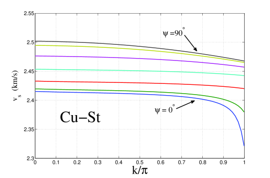
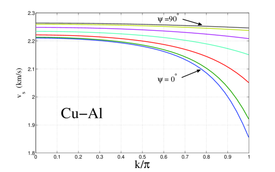
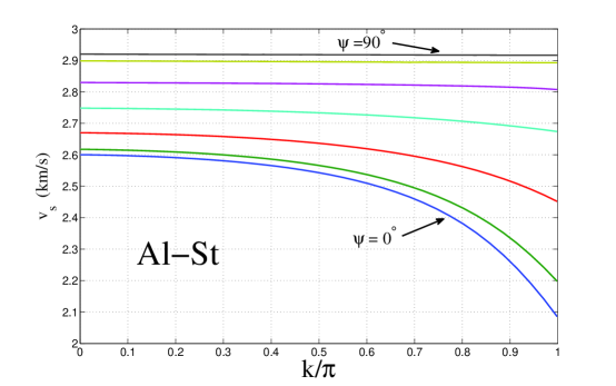
Figure 1: The surface wave speed $v_{s}$ for three laterally periodic bimaterials made of equal volume fractions of any two of copper, steel or aluminum (Cu, St, Al). The propagation direction $\mathbf{m}$ varies from $\psi=0$ (normal to the layers) to $\psi=90^{\circ}$ in increments of $15^{\circ}$.

6 Conclusions

Use of the matrix sign function provides a new and broader perspective of the surface wave problem in anisotropic media. It straightens out the methodology of the underlying matrix formalism and offers a direct method to compute the matrices involved. Starting from the defining property of the matrix sign function (11) we have obtained known relations for the Barnett-Lothe matrices, the impedance matrix and the dispersion equation for the surface wave speed, see eqs. (18), (21) and (23). These expressions are achieved using only the sign function of $i$ times the Stroh matrix $\mathbf{N}=\mathbf{K}\mathbf{N}^{T}\mathbf{K}$ without specifying its method of evaluation. An integral representation (13) for the matrix sign function, combined with the explicit structure of the Stroh matrix (27), leads immediately to the Barnett-Lothe integral relations (25). In this paper we have concentrated on using the matrix sign function for direct formulation of the dispersion equation, without discussing further properties of the Barnett-Lothe matrices which underlie the existence and uniqueness considerations in the surface wave theory [2, 3, 4]. We have constructed an explicit solution of the matrix Riccati equation for the impedance $\mathbf{Z}$ by rewriting the Riccati equation in a form (34) that involves the matrix sign function. Apart from providing for the first time a direct solution of the Riccati equation, the use of the matrix sign function shows how this nonlinear equation is intimately related with the Stroh matrix.

Perhaps the greatest advantage gained by using the matrix sign function is that it provides a natural formalism for framing the problem of subsonic surface waves in laterally periodic half-spaces which are inhomogeneous along the surface and uniform in the depth direction. We have shown how much of the structure for the homogeneous case carries over to the case of laterally periodic materials. For instance, the conditions for surface waves (63) and the form of the block matrices in the matrix sign function (62) mirror their counterparts for the homogeneous case, eqs. (22) and (25), respectively. Naturally, there are major differences between the problems. Conditions for the existence of surface waves in periodically inhomogeneous materials have only been recently established [30] but the methods that have been proposed for finding them are not as straightforward as for the homogeneous case. The approach that we have presented for the laterally periodic case, being linked via the matrix sign function to the well known formalism for the homogeneous half-space, offers, we believe, a clear and logical route for finding surface waves. Future work will examine this calculation method and the properties of the subsonic waves in more detail and will also consider supersonic solutions in the upper stopbands and passbands - the extension motivated by the classical paper by Alshits and Lothe [31].

Appendix: Sign function and related matrix functions

The matrix sign function of $\mathbf{M}$ is closely related to other standard matrix functions. The matrix projector functions $\mathbf{P}_{+}$ and $\mathbf{P}_{-}$ are defined

$$\mathbf{P}_{\pm}\boldsymbol{\xi}=\begin{cases}\boldsymbol{\xi},&\boldsymbol{\xi}\in\mathcal{L}_{\pm},\\ \mathbf{0},&\boldsymbol{\xi}\in\mathcal{L}_{\mp},\end{cases}\ \ \text{where}\ \mathcal{L}_{\pm}=\big{\{}\boldsymbol{\xi}:\,\mathbf{M}\boldsymbol{\xi}=\lambda\boldsymbol{\xi},\ \mathrm{Re}\,\lambda\,{\tiny\begin{matrix}>\\ <\end{matrix}}\,0,\big{\}},$$ (66)

and therefore

$$\operatorname{sign}\mathbf{M}=\mathbf{P}_{+}-\mathbf{P}_{-},\ \ \mathbf{I}=\mathbf{P}_{+}+\mathbf{P}_{-}\quad\Leftrightarrow\quad\mathbf{P}_{\pm}=\frac{1}{2}\mathbf{I}\pm\frac{1}{2}\operatorname{sign}\mathbf{M}.$$ (67)

The projector functions can be expressed via integration, e.g. [32]

$$\mathbf{P}_{\pm}=\frac{1}{2\pi i}\int_{C_{\pm}}\mathrm{d}z\,(z\mathbf{I}\mp\mathbf{M})^{-1}$$ (68)

where $C_{\pm}$ counter-clockwise encloses the finite right(left)-half plane $\{z:\,\mathrm{Re}\,(\pm z)>0,\ |z|<R\}$, $R$ arbitrarily large. The Schwartz-Christoffel transformation $z\to(z-1)(z+1)^{-1}$ reduces this to an integral around the unit circle

$$\mathbf{P}_{\pm}=\frac{1}{2\pi i}\int\limits_{|z|=1-0}\mathrm{d}z\,\big{(}z\mathbf{I}-\mathbf{F}^{\pm 1}\big{)}^{-1},\quad\mathbf{F}=(\mathbf{M}-\mathbf{I})(\mathbf{M}+\mathbf{I})^{-1}.$$ (69)

While $\mathbf{F}^{\pm 1}$ are singular if $\mathbf{M}$ possesses eigenvalues $\mp 1$, we note that (68) is unchanged for $\mathbf{M}\to a\mathbf{M}+ib\mathbf{I}$, $a,\,b\in\mathbb{R}$, $a>0$, and (69) is invariant for $\mathbf{F}\to(\mathbf{M}-\alpha\mathbf{I})(\mathbf{M}+\alpha^{*}\mathbf{I})^{-1}$, $\alpha\in\mathbb{C}$, $\mathrm{Re}\,\alpha>0$, and hence (69) can always be made regular by selecting $\alpha$ in the right half-plane. The integral representation (13) for the matrix sign function may be easily obtained from eqs. (67) and (69).

The disk function [11] is defined such that if $\mathbf{M}=\mathbf{U}$$\begin{pmatrix}\mathbf{J}_{1}&\mathbf{0}\\ \mathbf{0}&\mathbf{J}_{2}\end{pmatrix}$ $\mathbf{U}^{-1}$ where the eigenvalues of $\mathbf{J}_{1}$, $\mathbf{J}_{2}$ have magnitudes $<1$, $>1$, respectively, then $\operatorname{disk}\mathbf{M}=\mathbf{U}$$\begin{pmatrix}\mathbf{I}&\mathbf{0}\\ \mathbf{0}&\mathbf{0}\end{pmatrix}$$\mathbf{U}^{-1}$. It follows that

$$\operatorname{sign}\mathbf{M}=\mathbf{I}-2\operatorname{disk}\big{(}(\mathbf{M}-\mathbf{I})^{-1}(\mathbf{M}+\mathbf{I})\big{)}.$$ (70)

Acknowledgment

A.N.N. acknowledges support from Le Conseil Régional d’Aquitaine and the program CADMO of the cluster Advanced Materials in Aquitaine (GIS-AMA). A.A.K. acknowledges support from Mairie de Bordeaux.

References

• Stroh [1962] A. N. Stroh. Steady state problems in anisotropic elasticity. J. Math. Phys., 41:77––103, 1962.
• Barnett and Lothe [1973] D. M. Barnett and J. Lothe. Synthesis of the sextic and the integral formalism for dislocations, Greens functions, and surface waves in anisotropic elastic solids. Phys. Norv., 7:13–19, 1973.
• Lothe and Barnett [1976] J. Lothe and D. M. Barnett. On the existence of surface-wave solutions for anisotropic elastic half-spaces with free surface. J. Appl. Phys., 47(2):428–433, 1976.
• Chadwick and Smith [1977] P. Chadwick and G. D. Smith. Foundations of the theory of surface waves in anisotropic elastic materials. Adv. Appl. Mech., 17:303–376, 1977.
• Ting [1996] T. C. T. Ting. Anisotropic Elasticity: Theory and Applications. Oxford University Press, 1996.
• Barnett [2000] D. M. Barnett. Bulk, surface, and interfacial waves in anisotropic linear elastic solids. Int. J. Solids Struct., 37(1-2):45–54, 2000. doi: 10.1016/S0020-7683(99)00076-1.
• Norris and Shuvalov [2010] A. N. Norris and A. L. Shuvalov. Wave impedance matrices for cylindrically anisotropic radially inhomogeneous elastic materials. Q. J. Mech. Appl. Math., 63:1–35, 2010.
• Biryukov et al. [1995] V. Biryukov, Yu. V. Gulyaev, V. V. Krylov, and V. P. Plessky. Surface Acoustic Waves in Inhomogeneous Media. Springer, Berlin, 1995.
• Barnett and Lothe [1985] D. M. Barnett and J. Lothe. Free surface (Rayleigh) waves in anisotropic elastic half-spaces: The surface impedance method. Proc. R. Soc. A, 402(1822):135–152, 1985. doi: 10.2307/2397800.
• Higham [1994] N. J. Higham. The matrix sign decomposition and its relation to the polar decomposition. Linear Algebra Appl., 212/213:3–20, 1994.
• Higham [2008] N. J. Higham. Functions of Matrices: Theory and Computation. SIAM, Philadelphia, PA, 2008.
• [12] N. J. Higham. The Matrix Computation Toolbox. http://www.ma.man.ac.uk/~higham/mctoolbox.
• Kenney and Laub [1995] C. S. Kenney and A. J. Laub. The matrix sign function. IEEE Trans. Automat. Control, 40(8):1330–1348, 1995.
• Roberts [1980] J. D. Roberts. Linear model reduction and solution of the algebraic Riccati equation by use of the sign function. Int. J. Control, 32(4):677–687, 1980.
• Gundersen and Lothe [1987] S. A. Gundersen and J. Lothe. A new method for numerical calculations in anisotropic elasticity problemss. Phys. Stat. Sol. (B), 143(1):73–85, 1987. doi: 10.1002/pssb.2221430108.
• Condat and Kirchner [1987] M. Condat and H. O. K. Kirchner. Computational anisotropic elasticity. Phys. Stat. Sol. (B), 144(1):137–143, 1987. doi: 10.1002/pssb.2221440112.
• Koc et al. [1994] C. K. Koc, B. Bakkaloglu, and L. S. Shieh. Computation of the matrix sign function using continued fraction expansion. IEEE Trans. Automatic Control, 39(8):1644–1647, 1994. doi: 10.1109/9.310041.
• Ingebrigtsen and Tonning [1969] K. A. Ingebrigtsen and A. Tonning. Elastic surface waves in crystals. Phys. Rev., 184(3):942–951, 1969. doi: 10.1103/PhysRev.184.942.
• Honein et al. [1991] B. Honein, A. M. B. Braga, P. Barbone, and G. Herrmann. Wave propagation in piezoelectric layered media with some applications. J. Intell. Mater. Sys. Struct., 2(4):542–557, 1991. doi: 10.1177/1045389X9100200408.
• Wang and Rokhlin [2002] L. Wang and S. I. Rokhlin. Recursive impedance matrix method for wave propagation in stratified media. Bull. Seism. Soc. Am., 92:1129–1135, 2002.
• Shuvalov and Every [2002] A. V. Shuvalov and A. G. Every. Some properties of surface acoustic waves in anisotropic-coated solids, studied by the impedance method. Wave Motion, 36:257–253, 2002. doi: 10.1016/S0165-2125(02)00013-6.
• Hosten and Castaings [2003] B. Hosten and M. Castaings. Surface impedance matrices to model the propagation in multilayered media. Ultrasonics, 41(7):501–507, 2003. doi: 10.1016/S0041-624X(03)00167-7.
• Fu [2003] Y. B. Fu. Existence and uniqueness of edge waves in a generally anisotropic elastic plate. Q. J. Mech. Appl. Math., 56(4):605–616, 2003. doi: 10.1093/qjmam/56.4.605.
• Fu and Kaplunov [2012] Y. B. Fu and J. Kaplunov. Analysis of localized edge vibrations of cylindrical shells using the Stroh formalism. Math. Mech. Solids, 17(1):59–66, 2012. doi: 10.1177/1081286511412442.
• Biryukov [1985] S. V. Biryukov. Impedance method in the theory of elastic surface waves. Sov. Phys. Acoust., 31:350–354, 1985.
• Caviglia and Morro [2002] G. Caviglia and A. Morro. Wave reflection and transmission from anisotropic layers through Riccati equations. Q. J. Mech. Appl. Math., 55:93–107, 2002.
• Fu and Mielke [2002] Y. B. Fu and A. Mielke. A new identity for the surface-impedance matrix and its application to the determination of surface-wave speeds. Proc. R. Soc. A, 458(2026):2523–2543, 2002. doi: 10.2307/3067326.
• Kutsenko and Shuvalov [2013] A. A. Kutsenko and A. L. Shuvalov. Shear surface waves in phononic crystals. J. Acoust. Soc. Am., 133(2):653–660, 2013. doi: 10.1121/1.4773266.
• Shuvalov [2003] A. L. Shuvalov. A sextic formalism for three-dimensional elastodynamics of cylindrically anisotropic radially inhomogeneous materials. Proc. R. Soc. A, 459(2035):1611–1639, 2003.
• Hu et al. [2012] L. X. Hu, L. P. Liu, and K. Bhattacharya. Existence of surface waves and band gaps in periodic heterogeneous half-spaces. J. Elasticity, 107(1):65–79, 2012. doi: 10.1007/s10659-011-9339-0.
• Al’shits and Lothe [1981] V. I. Al’shits and J. Lothe. Comments on the relation between surface wave theory and the theory of reflection. Wave Motion, 3:297––310, 1981.
• Bai and Demmel [1998] Z. Bai and J. Demmel. Using the matrix sign function to compute invariant subspaces. SIAM J. Matrix Anal. Appl, 19:205–225, 1998.