Linking dynamical and functional properties of intrinsically bursting neurons

Abstract

Several studies have shown that bursting neurons can encode information in the number of spikes per burst: As the stimulus varies, so does the length of individual bursts. The represented stimuli, however, vary substantially among different sensory modalities and different neurons. The goal of this paper is to determine which kind of stimulus features can be encoded in burst length, and how those features depend on the mathematical properties of the underlying dynamical system. We show that the initiation and termination of each burst is triggered by specific stimulus features whose temporal characteristsics are determined by the types of bifurcations that initiate and terminate firing in each burst. As only a few bifurcations are possible, only a restricted number of encoded features exists. Here we focus specifically on describing parabolic, square-wave and elliptic bursters. We find that parabolic bursters, whose firing is initiated and terminated by saddle-node bifurcations, behave as prototypical integrators: Firing is triggered by depolarizing stimuli, and lasts for as long as excitation is prolonged. Elliptic bursters, contrastingly, constitute prototypical resonators, since both the initiating and terminating bifurcations possess well-defined oscillation time scales. Firing is therefore triggered by stimulus stretches of matching frequency and terminated by a phase-inversion in the oscillation. The behavior of square-wave bursters is somewhat intermediate, since they are triggered by a fold bifurcation of cycles of well-defined frequency but are terminated by a homoclinic bifurcation lacking an oscillating time scale. These correspondences show that stimulus selectivity is determined by the type of bifurcations. By testing several neuron models, we also demonstrate that additional biological properties that do not modify the bifurcation structure play a minor role in stimulus encoding. Moreover, we show that burst-length variability (and thereby, the capacity to transmit information) depends on a trade-off between the variance of the external signal driving the cell and the strength of the slow internal currents modulating bursts. Thus, our work explicitly links the computational properties of bursting neurons to the mathematical properties of the underlying dynamical systems.

1 Introduction

In the absence of noise, intrinsically bursting neurons generate periodic bursts. Periodic activity may serve to control basic physiological functions, as respiration (Smith et al.,, 1991), digestion movements (Selverston and Miller,, 1980), egg laying (Alevizos et al.,, 1991), or insulin secretion (Meissner and Schmelz,, 1974). It cannot, however, transmit information. As input noise increases, bursting responses become variable (Kuske and Baer,, 2002; Su et al.,, 2004; Pedersen and Sørensen,, 2006; Channell et al.,, 2009), and the number of spikes per burst may fluctuate in time. Experimental studies performed in different sensory domains have demonstrated that often, variability in burst length reflects variability in specific transient features of a time-dependent stimulus, for example, the orientation of a visual stimulus, (Martinez-Conde et al.,, 2002), the loudness of an auditory stimulus, (Eyherabide et al.,, 2009), or the velocity of a somatosensory stimulus (Arganda et al.,, 2007). Bursts of different lengths, therefore, are selective to different stimulus features. This paper aims at understanding which properties of bursting dynamics determine stimulus selectivity.

The mapping between burst length and stimulus features is likely to depend on the biophysical properties of the neuron, such as its morphology, the types of ionic channels located on the cellular membrane, their kinetics and their spatial distribution. These properties may vary continuously in a complex, high-dimensional space. Yet, from the dynamical point of view, bursting neurons only display a finite number of qualitatively different behaviors, depending on the bifurcations governing the underlying dynamical system (Izhikevich,, 2007). Previous studies (Izhikevich and Hoppensteadt,, 2004; Mato and Samengo,, 2008) have demonstrated that the computational properties of non-bursting cells, in particular their selectivity to specific stimulus features, are determined by the bifurcation governing the onset of firing. We here hypothesize that a similar link between dynamical and computational properties can also be established for bursting neurons.

By combining all the possible bifurcations that can initiate or terminate spiking, one can in principle construct 120 types of bursting neurons (Izhikevich,, 2007). Most of these types, however, have never been observed experimentally, and some of them appear only rarely. We therefore focus on the three most ubiquitous types: parabolic, square-wave and elliptic. In order to explore the selectivity of each type, we simulate their activity when driven with a noisy input current and perform a statistical analysis of the stimulus stretches inducing bursting, obtaining the so-called preferred stimuli. To characterize the input-output mapping of each type, we search for the amplitude and frequency properties of the preferred stimuli and interpret those properties in terms of the underlying bifurcations.

In order to determine whether additional biological details also shape stimulus selectivity, each type of burster is represented with three different models, capturing different amounts of biophysical properties: a minimal normal-form model, a minimal conductance-based model, and a detailed conductance-based model. The main result is that stimulus selectivity is mainly shaped by the bifurcation structure of the burster, and is roughly independent of further details. The present study thus links the dynamics and the computational characteristics of bursting neurons.

Results

Variability of bursting responses

When driven with constant currents, intrinsically bursting neurons tend to generate periodic responses. In the presence of noisy inputs, however, some variability in the number of spikes per burst may appear, as well as in the duration of the intra-burst and the inter-burst intervals. The amount of variability is not fixed, and example neurons can be found whose responses are remarkably periodic, or remarkably variable. We begin by identifying the factors determining the degree of periodicity.

The variables involved in the dynamical description of bursting can be separated into two classes: fast variables and slow variables (Rinzel,, 1987). The former participate in spike generation, and vary in time scales of the order of 1 ms. The latter vary at a much slower time scale (tens or hundreds of milliseconds). The evolution of the membrane potential is governed by equations of the form

$$\frac{{\rm d}V}{{\rm d}t}=f(V)+\sum_{i}I_{\rm spike}^{i}+\alpha\sum_{j}I_{\rm burst}^{j}+I_{\rm ext},$$ (1)

where $f$ is a function of the membrane potential (see Methods), $I_{\rm spike}^{i}$ and $I_{\rm burst}^{j}$ represent the fast and slow currents respectively, $I_{\rm ext}$ is the external stimulus, and $\alpha$ is the coupling constant regulating the degree of coupling between fast and slow variables. The evolution of the fast and slow currents is determined by additional variables, governed by additional equations whose functional form depends on the degree of biological detail (see Methods).

When fast and slow time-scales are well separated, slow variables define an almost constant current that competes with the external inputs synapsing on the neuron. Throughout this paper, the external current is modeled as

$$I_{\rm ext}=I_{0}+\sigma\xi(t),$$ (2)

where $I_{0}$ is a constant DC, $\xi(t)$ is a stochastic term of zero mean and unit variance (see Methods) and $\sigma$ represents the noise intensity.

In Figure  1 we show that the amount of variability in bursting responses is determined by a trade-off between the amount of noise $\sigma$ in the input signal and the strength $\alpha$ of the coupling between fast and slow variables. One can therefore increase the response variability by either increasing the amount of noise or decreasing the coupling between fast and slow variables. Panel (a) represents the noiseless situation. The inter-spike interval (ISI) distribution contains two sharp peaks, the first one corresponding to the intra-burst intervals and the second one to the inter-burst silent periods. The voltage trace looks perfectly regular. As we move to panels (b) and (c), the noise $\sigma$ increases. ISI distributions become wider, and voltage traces appear more disordered. If the amount of noise remains fixed, however, one can also vary the degree of disorder by modifying the coupling strength $\alpha$. The larger the coupling, the larger the contribution of the slow variables to the evolution of the membrane voltage. Noise therefore exerts a comparatively weaker influence. Responses in panels (d) and (e) are calculated with the same $\sigma$ as in (b). However, increasing $\alpha$ (panel (d)) introduces order, resulting in a sharper ISI distribution and more regular spiking. Instead, decreasing $\alpha$ (panel (e)) modifies the responses in a way that is similar to the one obtained with increased noise (compare with panel (c)). Therefore, coupling strength and noise act as opposite forces in determining the amount of variability.

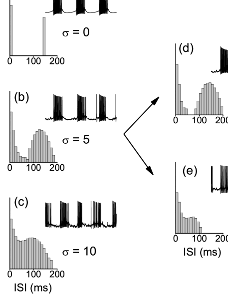
Figure 1: Periodicity vs. variability of bursting responses. A parabolic minimal conductance-based model (see Methods) is driven with a noisy input current of standard deviation $\sigma$ (expressed in $\mu$A ms^1/2/cm²) and mean value $I_{0}$. The magnitude of $I_{0}$ was chosen to maintain the average firing rate at 75 Hz. (a) ISI distribution in logarithmic scale and example voltage trace for the noiseless case. The spike train is perfectly periodic. (b) and (c): increasing amounts of noise are employed. The coupling strength is equal as in (a). (d) and (e): The amount of noise is fixed at 5 $\mu$A ms^1/2/cm², but the coupling strength is increased in (d), and decreased in (e), resulting in more ordered and disordered responses, respectively. Noise and coupling strength thus act as opposite forces in determining response variability.

Classification of bursting models in terms of their bifurcations

In an adiabatic approximation, slow variables can be considered almost constant in short intervals. At the fast time scales, hence, slow variables operate as bifurcation parameters of the fast subsystem. One bifurcation initiates bursting and another one terminates it. The average values of the fast variables, in turn, self-consistently modulate the slow subsystem at longer time scales. The bifurcation structure of different bursting neurons allowed Rinzel, (1987) to classify bursters as parabolic, square-wave or elliptic.

In parabolic bursters, the initiation and termination of spiking within each burst is governed by a saddle-node bifurcation on the invariant circle of the fast subsystem. These transitions are characterized by large-amplitude and low-frequency oscillations. As a result, the first and last spike of the burst display ample voltage deflections. The ISIs, in turn, are modulated throughout the duration of the burst, displaying a slow-fast-slow sequence. This modulation gives parabolic bursts their name: The sequence of ISIs in a burst is a parabolic-shaped function of time. These features are displayed in Figure 2 (a1), for the minimal conductance-based model. The minimal normal form and the detailed con-ductance-based models are topologically equivalent. Figure 2 (a2) shows the phase portrait of the parabolic burster projected on the space defined by the two fast variables, and one of the two slow variables.

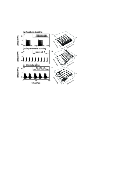
Figure 2: Properties of different bursting models. Minimal conductance-based models were stimulated with a constant external current, and the voltage trace is displayed (left) as well as a phase-space trajectory (right). Different types of bursters exhibit qualitatively different traces. (a): Parabolic burster. (a1): $I_{0}=5\mu$A/cm². (a2): $I_{0}=3\mu$A/cm². (b): Square-wave burster. (b1) and (b2): $I_{0}=6\mu$A / cm². C: Elliptic burster. (c1): $I_{0}=55.5\mu$A / cm². (c2): $I_{0}=52\mu$A / cm². Insets: amplification of the voltage trace in a single burst.

In square-wave bursters, the initiation of spiking is governed by a fold bifurcation, that is, a saddle-node bifurcation away from the invariant circle. This transition is characterized by large amplitude and high-frequency spiking. Burst termination occurs through a homoclinic bifurcation, distinguished by large amplitude and low frequency fluctuations. Accordingly, the voltage trace in Figure 2 (b1) shows a deceleration of spiking as the burst proceeds, without a significant attenuation of the height of voltage upstrokes. Figure 2 (b2) displays a burst in the 3-dimensional phase space.

In elliptic bursters, the initiation of spiking is governed by two bifurcations, one of them responsible for the loss of stability of the fixed point representing the resting state, and the other for the creation of two limit cycles, the stable one representing the spiking state, and an additional unstable cycle. The fixed point looses stability through a subcritical Hopf bifurcation, and at approximately the same critical current value, the two limit cycles are created through a fold bifurcation of cycles. The combination of these two bifurcations is called a Bautin bifurcation (Arnold,, 2008). Burst termination involve the same two bifurcations occurring in the reverse direction: The fixed point becomes stable through a Hopf bifurcation and the limit cycles disappear through a fold bifurcation of cycles. Elliptic bursts are characterized by large-amplitude and high-frequency fluctuations. As exemplified in the inset of Figure 2 (c1), the voltage trace exhibits subthreshold oscillations between bursts, characteristic of Hopf bifurcations. At spiking onset, the voltage fluctuations suddenly increase in amplitude and switch to the frequency of the limit cycle created through the fold bifurcation of cycles. The subthreshold and suprathreshold frequencies are associated with two different attractors, and therefore, do not necessarily coincide. The termination process is qualitatively similar. Figure 2 (c2) shows the typical subthreshold oscillations observed in elliptic bursters at the beginning and at the end of each burst appearing as 3-dimensional spirals.

Bursting responses obtained with simple stimuli

Before studying systematically bursting activity in response to stochastic inputs we briefly survey their behavior when driven with simple stimuli, as constant or sinusoidal input currents.

When constant currents are employed ($\sigma$ = 0, in Equation 2) the number of spikes per burst typically grows as a function of $I_{0}$, though not always monotonically (Figure 3 (a1, b1, c1)). In each case, $I_{0}$ is varied between a minimum value, below which no spiking occurs, and a maximum value, beyond which spiking is no longer structured in bursts, i.e., tonic spiking begins. The mean intra-burst frequency remains roughly unchanged as $I_{0}$ varies (panels (a2, b2, c2)). A constant mean intra-burst frequency, however, does not imply that all the ISIs inside the burst are equal. Parabolic and square-wave bursters, in fact, modulate their ISIs throughout the burst, so the standard deviation of the intra-burst frequency (shaded areas in Figure 3 (a2, b2, c2)) is large, at least, when compared to elliptic bursters. The dented structure in panels (a2, b2, c2) corresponds to the steps in panels (a1, b1, c1): When the number of spikes per burst increases in one unit, an extra spike is packed into each burst, so the intra-burst ISIs diminish, and so does the standard deviation. Finally, the inter-burst frequency grows with $I_{0}$ (panels (a3, b3, c3)) with only small fluctuations each time the number of spikes per burst increases.

When driven with subthreshold stimuli, parabolic and square-wave bursters do not display subthreshold oscillations, since their fixed points are foci. Elliptic bursters, instead, oscillate at the frequency associated with the elliptic fixed point (see Figure 2(c)). Therefore, when driven with subthreshold sinusoidal stimuli, elliptic bursters may resonate with the input frequency, as evidenced in the ZAP (impedance (Z) amplitude (A) profile (P), (Gimbarzevsky et al.,, 1984; Puil et al.,, 1986) depicted in Figure 3c. Parabolic (a4) and square-wave (b4) bursters have maximal voltage amplitude for zero-frequency stimulation, whereas elliptic bursters (c4) have a prominent resonance at 328 Hz.

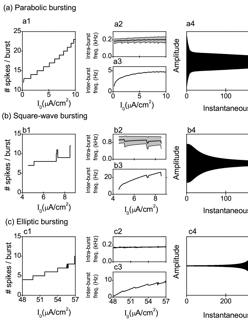
Figure 3: Response characteristics of different types of bursting neurons. Minimal conductance-based models are stimulated with constant currents, and the number of spikes per burst (a1, b1, c1) is measured as a function of the input strength. The intra (a2, b2, c2) and inter-burst (a3, b3, c3) frequencies are calculated as the inverse of the intra and inter-burst periods. The envelope of the voltage response to ZAP input currents is an estimation of the resonance curve for each model. Subthreshold values of $I_{0}$ have been used, near to the firing threshold. (a4): $I_{0}=0.1\mu A/$ cm², fluctuations of amplitude $I_{1}=0.01\mu A/$ cm². (b4): $I_{0}=4\mu A/$ cm², $I_{1}=0.2\mu A/$ cm². (c4): $I_{0}=44\mu A/$ cm², $I_{1}=0.5\mu A/$ cm².

Classification of bursting models in terms of their degree of biological detail

We now turn to the analysis of stimulus selectivity of different bursting models. Our working hypothesis is that the stimulus features associated with bursts of a given length depend on the dynamical properties of the bifurcations associated with the initiation and termination of bursts. Other biophysical properties beyond the bifurcation should only weakly affect stimulus selectivity. To test the hypothesis, we simulated each type of burster with three different models. The simplest models are formulated in terms of minimal normal-forms. They involve dimensionless variables, only loosely related to biophysical quantities. These models are designed to capture the topological properties of each bifurcation type in their purest form. As a first step towards biological realism we also used minimal conduct-ance-based models, formulated in terms of variables representing real biological quantities, though not intended to represent any specific neuron. These models were introduced by Izhikevich, (2007) as the simplest conductance-based models with the bifurcations of real neurons. Finally, in an attempt to also include realistic neural models, we simulated detailed conductance-based models, proposed by Chay and Cook, (1988), and further analyzed by Bertram et al., (1995). These models represent pancreatic neurons that, depending on the value of the parameters, can exhibit parabolic, square-wave, or elliptic bursting.

Stimulus selectivity of different bursting models

Stimulus selectivity was evaluated by calculating the burst-triggered average (BTA) of bursts containing a fixed number of spikes. To do so, we simulated several bursting models, differentiated by their type (parabolic, square-wave and elliptic) or by the amount of biophysical detail (minimal normal forms, minimal conductance-based models, and detailed conductance-based models). In each case, bursts were identified by analyzing the ISIs in the spike train (see Methods). BTAs were calculated by pooling all the stimulus segments surrounding the generation of bursts of exactly $n$ spikes and averaging them together. Therefore, each $n$-BTA represents the average stimulus around bursts of $n$ spikes. We define $t=0$ as the time of burst initiation.

In Figure 4, we show the results for the three parabolic models. Different curves correspond to bursts containing different number of spikes. The stimulus parameters are given in Tables 1-3. Although the detailed shape of the BTAs varies with the amount of biological detail, there are some general trends that are shared by all three models. In all cases, bursting is preceded by a marked increase in $I_{\rm ext}$. In the minimal normal form and minimal conductance models (panels (a) and (b)), bursts are triggered by a peak that starts rising some 10 ms before burst onset. The detailed conductance-based model (panel (c)) is governed by much slower time constants, and the peak begins to become noticeable 1-2 seconds before burst initiation, an interval 2 orders of magnitude longer than in the two preceding cases. Hence, the temporal scale of the structures in the BTA is determined by the details of the model, and not by the type of bifurcation.

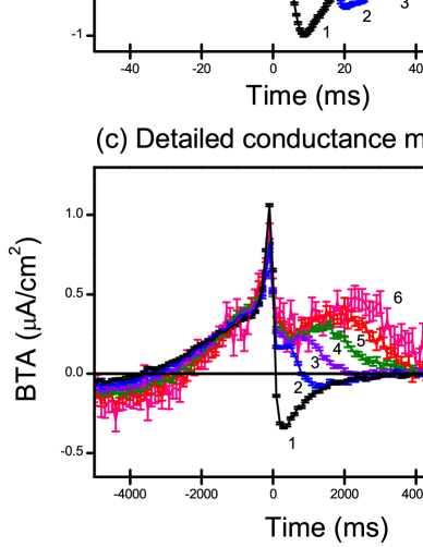
Figure 4: BTA of parabolic bursters. Burst onset is at time zero. (a): Minimal normal form. (b): Minimal conductance-based model. (c): Detailed conductance-based model. Error bars represent the error of the mean. Different curves correspond to bursts containing different number of spikes. In the three models, bursts are triggered by a strong, depolarizing stimulus upstroke. The burst is prolonged as long as the excitation is maintained.

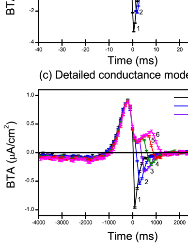
Figure 5: BTA of square-wave bursters. Burst onset is at time zero. Error bars represent the error of the mean. Different curves correspond to bursts containing different number of spikes. (a): Minimal normal form. (b): Minimal conductance-based model. (c): Detailed conductance-based model. In the three models, bursts are triggered by a small hyperpolarization, followed by a strong, depolarizing stimulus upstroke. To sustain the burst beyond 3 spikes, a second upstroke is required.

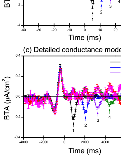
Figure 6: BTA of elliptic bursters. Burst onset is at time zero. Error bars represent the error of the mean. Different curves correspond to bursts containing different number of spikes. (a): Minimal normal form. Arrows show the position of the upstroke that terminates the burst. (b): Minimal conductance-based model. (c): Detailed conductance-based model. In (b) and (c) arrows show the position of the downstroke that terminates the burst. In the three models, bursts are triggered by an oscillating input current of a well-defined frequency. Bursts are maintained until the input signal inverts its phase.

In the three models, for $t<0$ all curves overlap. No matter how many spikes are contained in each burst, bursts are always triggered by the same type of stimulus deflection. Hence, at the time of burst initiation, there is no way to predict how many spikes the burst will contain based on the shape of the stimulus thus far. To discriminate the stimuli associated with short and long bursts, one must evaluate the shape of $I_{\rm ext}$ for positive times. Long bursts appear in response to sustained stimulation beyond burst initiation. Short bursts are terminated as soon as the stimulus drops. In the normal form (panel (a)) and in the minimal conductance-based model (panel (b)), oscillations appear during sustained stimulation, and including the first large peak, there is one oscillation per spike in the burst. However, this characteristic is not a general property of all parabolic models, since it is not observed in the detailed conductance-based model (panel (c)).

These characteristics may or may not appear in other types of bursting neurons. In Figure 5 we show the BTAs corresponding to square-wave bursters. Also here bursts are triggered by a sharp, positive stimulus deflection, and once again, up to the time of burst onset ($t\leq 0$) the shape of the stimulus does not suffice to predict how long the burst will last. This time, we can also see a shallow hyperpolarizing phase preceding the burst-triggering peak. As before, long bursts are associated with prolonged stimulation, whereas short bursts require a sharp downstroke to terminate. The shape of both the prolonged stimulation and the downstroke is remarkably similar across different models (panels (a), (b), and (c)). However, it differs from the shapes observed in the parabolic case (Figure 4). Long bursts in square-wave bursters require stimuli containing two separate peaks. In order to sustain spiking beyond the mean burst length (3 spikes per burst, for the mean currents used in Figure 5), an additional positive derivative in the current is required. This stimulus upstroke marks the initiation of the second peak in the BTA. In the minimal normal form, the second peak begins 0.5 ms after burst onset, and in the other two models, at 1 and 200 ms. In the three models, the timing between burst initiation and the beginning of the second peak coincides with the period of the spiking limit cycle at burst onset. Hence, to get long bursts we need a 2-peak oscillation in the stimulus whose frequency coincides with the frequency of the limit cycle of the fold bifurcation initiating spiking. The second peak in the stimulus therefore begins to be noticeable at the time when the second spike of the burst is fired.

Elliptic bursting is markedly different from the previous two. In Figure 6 we see that the BTAs of the three elliptic models contain a pronounced oscillatory structure. The frequency of the oscillations remains roughly constant throughout the whole of the BTA in the normal form model ((a)). In the conductance-based models (panels (b) and (c)), the frequency diminishes after burst initiation. In all three cases, the frequency before burst initiation coincides with the frequency associated with the spiral fixed point, defined by the imaginary part of the eigenvalue loosing stability. The frequency after burst initiation coincides with the frequency of the spiking limit cycle. The two frequencies coincide in the case of the normal form (a), but do not coincide in the conductance-based models (b) and (c).

Burst initiation is triggered by gradually amplifying stimulus oscillations. Once again, the BTAs corresponding to bursts of different duration coincide for $t\leq 0$. Burst termination may be due to a marked upstroke (panel (a)) or downstroke (panels (b) and (c)), as indicated by the arrows in Figure 6. In all cases, the terminating feature (be it an upstroke or a downstroke) is out of phase with respect to the ongoing oscillation. Hence, burst termination is governed by a sudden phase inversion in the stimulus. The fact that the phase inversion may appear either as a peak or a trough implies that the extinction of the burst does not depend on the sign of the stimulus deflection, but rather, on the phase inversion.

Dependence on simulation parameters

Stimulus selectivity varies in a systematic fashion when the baseline current $I_{0}$, the amount of noise $\sigma$, and the coupling strength $\alpha$ are modified. In Figure 7 we display the BTAs of the normal-form models previously shown in Figures 4-6 but now for different coupling strengths $\alpha$.

In parabolic and square-wave bursters, as $\alpha$ changes, the family of BTAs obtained for different $n$ values shifts either upward or downward. The direction of the shift is determined by the mean number of spikes per burst $\langle n\rangle$, which in turn, is a function of $\alpha$. For a given $\alpha$, the mean duration of each burst is $\langle n\rangle$. Bursts with $n>\langle n\rangle$ (panels (a1) and (b1)) require sustained excitation in order to last longer than the typical length $\langle n\rangle$. Bursts with $n<\langle n\rangle$ (panels (a3) and (b3)), instead, require a prompt downstroke to terminate firing rapidly, before the length $\langle n\rangle$ is reached. In panels a2 and b2, $\langle n\rangle\approx 3$, so some of the curves display downstrokes (those with $n<\langle n\rangle$) and others sustained excitation (those with $n>\langle n\rangle$).

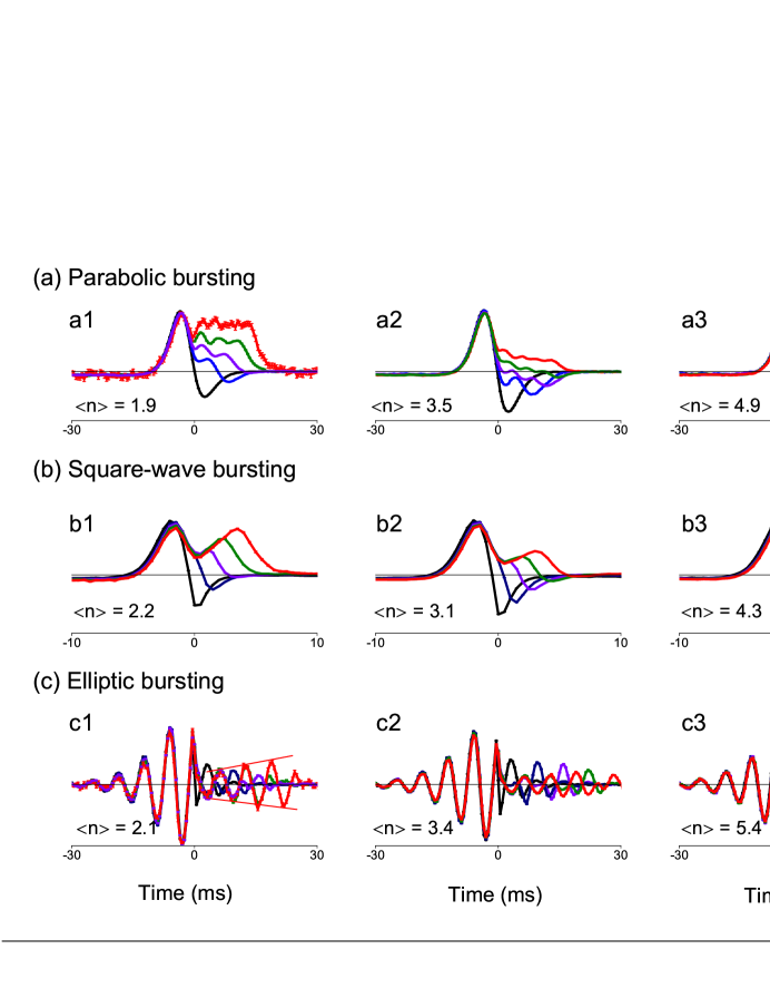
Figure 7: BTAs for different coupling strengths $\alpha$ in normal-form models. Burst onset is at time zero. Error bars represent the error of the mean, sometimes too small to be visible. Different curves correspond to bursts containing different number of spikes ranging from $n=1$ to $n=5$ with the same color code as in Figures 4-6. (a) Parabolic bursting. a1: $\alpha=0.91$. a2: $\alpha=1$. a3: $\alpha=1.05$. (b) Square-wave bursting. b1: $\alpha=1.81$. b2: $\alpha=1$. b3: $\alpha=0.55$. (c) Elliptic bursting. c1: $\alpha=1.6$. c2: $\alpha=1$. c3: $\alpha=0.6$.

The relationship between $\alpha$ and $\langle n\rangle$ is not universal, i.e., different models show different trends. For example, increasing $\alpha$ results in a larger $\langle n\rangle$ in the square-wave model of Figure 7 (b), and a smaller $\langle n\rangle$ in the parabolic case of panel (a). Yet, in conductance-based models different trends may be found. The key factor determining whether $\langle n\rangle$ grows or diminishes with $\alpha$ is the sign of the average value of the slow current. The current $I_{\rm burst}$ exerts an influence on the fast sub-system that may be excitatory, inhibitory or neutral on average. In the parabolic model of Figure 7 (a) $I_{\rm burst}$ is excitatory. In the square-wave model (panel b), $I_{\rm burst}$ is inhibitory. Yet other models sharing the same bifurcations can be engineered with mean slow currents of opposite sign. Therefore, the relationship between $\alpha$ and $\langle n\rangle$ is not a universal property of all parabolic or square-wave models. Once the relationship is given, however, stimulus selectivity varies systematically as a function of $\alpha$.

Elliptic bursters behave in the same way, though the effect is less visible by naked eye, because prolongation and termination features are not easily separated visually. After burst onset, in-phase oscillations constitute prolongation features. The last oscillation, appearing with inverted phase is a terminating feature. When $n>\langle n\rangle$, bursts need to be prolonged beyond their natural duration. The prolongation becomes increasingly difficult as time goes by, so the oscillations sustaining bursts during positive times increase in amplitude as the burst proceeds (marked with two lines in Figure 7 c1 for $n$ = 5). The terminating feature is instead small. When $n<\langle n\rangle$, bursts need to be terminated before they reach their natural duration. The termination signal must be particularly strong when the natural duration is large (large $\langle n\rangle$). Therefore, the out-of-phase terminating feature in c3 (marked with arrows, one for each $n$) has a larger amplitude than in c1.

Stimulus selectivity also varies when other parameters are modified, as for example the stimulus mean $I_{0}$ or the standard deviation $\sigma$. In these cases, again, the critical factor is how these variations affect $\langle n\rangle$. Changes in $\langle n\rangle$ originated in changes in $I_{0}$ produce BTAs that, when arranged in increasing value of $\langle n\rangle$, are in all similar to the ones depicted in Figure 7. Changes in $\sigma$ also give rise to the same phenomena, with one additional effect: For large $\sigma$, BTAs have less memory of events occurring in the distant past or distant future. As a consequence, BTAs look the same as in Figure 7, but with a damped envelope that gradually decays for positive and negative times.

Independent components in stimulus selectivity

The BTA is the average stimulus preceding a burst. When a single burst is generated, the triggering stimulus typically differs from the BTA up to a certain degree. Therefore, one can calculate not only the mean stimulus of each $n$, but also the variability around the mean. When studying a collection of scalar quantities, variability is captured by the standard deviation. With vectorial quantities, a single number does not suffice to describe variability, since there are many possible directions in which fluctuations may appear. Covariance analysis provides a tool for detecting the stimulus directions where uncorrelated variations are observed. Noticeably, variations are particularly large, or particularly small in only a few directions. These are the so-called relevant directions: Stimulus directions where the standard deviation of the burst-triggering ensemble is either larger or smaller than in the prior stimulus (see Methods). Covariance analysis also provides a systematic procedure to reveal these relevant directions (Samengo and Gollisch,, 2013). Here, the analysis is carried out for each intra-burst spike count $n$. The stimulus segments preceding bursts containing exactly $n$ spikes are identified, and their temporal correlations are captured by the covariance matrix. The eigenvectors of this matrix represent the relevant features, and the corresponding eigenvalues provide a quantitative measure of the variance of the data in these directions (see Methods). Typically, most burst-eliciting stimulus directions have approximately the same variance as the total stimulus, and only a few depart noticeably from the general trend. The eigenvectors associated with outlier eigenvalues constitute the relevant stimulus directions.

In Figure 8, we show the eigenvalues and eigenvectors of the normal form of a parabolic burster. The two most prominent outlier eigenvalues are ${\rm e}_{199}$ and ${\rm e}_{200}$, and both of them have decreased variance. In panels (b-c) we see the eigenvectors associated with each of the outlier eigenvalues, for bursts containing different numbers of spikes.

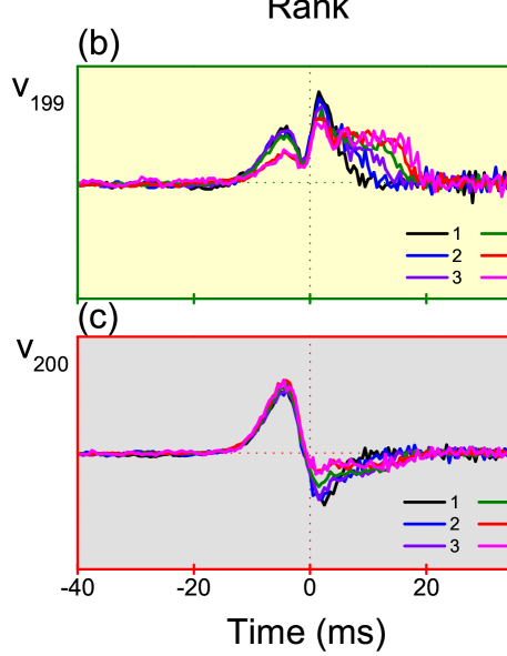
Figure 8: Covariance analysis of a parabolic burster. Data obtained by simulation of the minimal normal-form model. (a): Example spectrum of eigenvalues for stimulus segments triggering bursts containing 5 spikes. The two most clear outliers ($e_{199}$ and $e_{200}$) are marked. Insets: eigenvector corresponding to each eigenvalue. (b-c): Eigenvectors associated with outlier eigenvalues, for bursts containing $n$ spikes (one curve for each value of $n$). Burst onset is at time zero. Eigenvector ${\rm v}_{200}$ only contains stimulus features initiating the burst, whereas ${\rm v}_{199}$ mainly describes structures needed to sustain and terminate the burst.

Eigenvector ${\bf v}_{200}$ is the most significant relevant feature, since its eigenvalue has the largest deviation from unity. Its shape strongly resembles the BTA (Figure 4), except for the lack of a plateau at positive times, for long bursts. There is virtually no difference in the shape of the vectors corresponding to bursts containing different numbers of spikes. Variations in this direction capture the fluctuations in the stimulus deflection triggering bursts. Eigenvector ${\bf v}_{1}$ is therefore involved in shaping burst initiation, but it contains no features related to burst termination.

Parabolic bursting lasts for as long as the stimulus depolarizes the cell (Figure 4). That is, longer bursts are associated with more prolonged stimulation. Eigenvector ${\bf v}_{199}$ captures these differences: In Figure 8(b), we see that bursts containing a single spike are briefly stimulated, whereas 6-spikes bursts are driven for almost 20 ms after burst onset. Therefore, eigenvector ${\bf v}_{199}$ crucially captures burst termination.

Since burst initiation and burst termination are described by two different eigenvectors (${\bf v}_{200}$ and ${\bf v}_{199}$, respectively), these two processes are uncorrelated: Fluctuations in the features associated with burst initiation are not correlated with fluctuations responsible for burst termination.

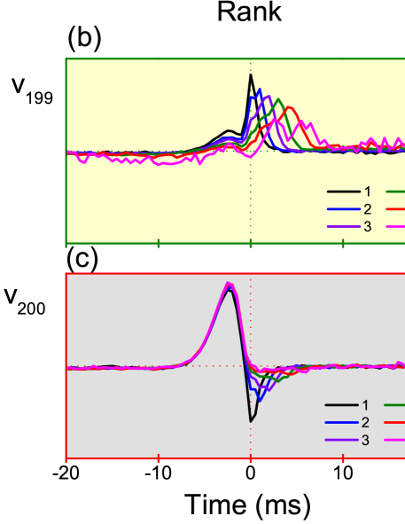
Figure 9: Covariance analysis of a square-wave burster. Data obtained by simulation of the minimal normal-form model. (a): Example spectrum of eigenvalues for stimulus segments triggering bursts containing 4 spikes. Two outliers ($e_{199}$ and $e_{200}$) are visible. Insets: eigenvector corresponding to each eigenvalue. (b-c): Eigenvectors associated with outlier eigenvalues for bursts containing $n$ spikes (one curve for each value of $n$). Burst onset is at time zero. Eigenvector ${\rm v}_{200}$ contains stimulus features initiating the burst, whereas ${\rm v}_{199}$ describes the structures needed to sustain and terminate the burst.

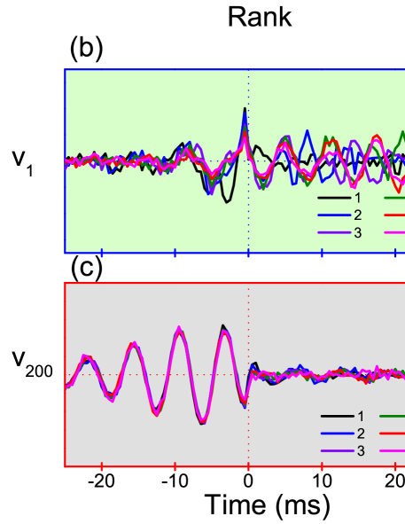
Figure 10: Covariance analysis of an elliptic burster. Data obtained by simulation of the minimal normal-form model. (a): Example spectrum of eigenvalues, for stimulus segments triggering bursts containing 4 spikes. Two outliers (${\rm v}_{1}$ and ${\rm v}_{200}$) are visible. Insets: eigenvectors corresponding to each eigenvalue. (b, c): Eigenvectors associated with outlier eigenvalues, for bursts containing $n$ spikes (one curve for each value of $n$). Burst onset is at time zero. Eigenvector ${\rm v}_{200}$ contains stimulus features initiating the burst, whereas ${\rm v}_{1}$ describes the structures needed to sustain and terminate the burst.

A similar situation is found for square-wave and elliptic bursters, as shown in Figures 9 and 10. In both cases, eigenvector ${\bf v}_{200}$ describes the shape of the stimulus features initiating the burst. In the case of a square-wave burster (Figure 9(c)), this feature is a depolarizing upstroke, whereas in the elliptic case (Figure 10(c)), bursting is initiated by an oscillation whose frequency coincides with the subthreshold resonance frequency of the cell. The remaining eigenvector (${\bf v}_{199}$ in the square-wave burster, and ${\bf v}_{1}$ in the elliptic case) represents the stimulus features terminating the burst.

When working with conductance-based models, similar results are obtained: Stimulus features responsible for burst initiation and termination tend to appear in separate eigenvectors. The eigenvectors responsible for burst initiation remain unchanged when $n$ is varied. Those responsible for burst prolongation or termination, instead, mark the differences in stimulus selectivity of different $n$ values.

Discussion

Initial studies on bursting neurons showed that they fire in a stereotyped fashion, and that regular bursting appears spontaneously even in culture tissue (Chagnac Amitai and Connors,, 1989; Silva et al.,, 1991; Steriade,, 1991; Agmon and Connors,, 1992). Bursting was thus assumed to serve as a pacemaker signal in drowsy or anesthetized states (Steriade,, 1991; Steriade et al.,, 1993), but could not encode transient information, since a perfectly periodic signal has zero information rate. More recent studies, however, have shown that the number of spikes per burst may encode specific properties of the input stimulus. In sensory systems, these include the visual system of mammals (DeBusk et al.,, 1997; Martinez-Conde et al.,, 2002), the auditory system of insects (Eyherabide et al.,, 2008, 2009; Marsat and Pollack,, 2010), the somatosensory system of leech (Arganda et al.,, 2007) and the olfactory system of rodents (Cang and Isaacson,, 2003). Theoretical studies have shown that the number of spikes per bursts encode the slope (Kepecs et al.,, 2002) or the phase (Samengo and Montemurro,, 2010) of the input current driving a cell.

Our analysis shows that these two behaviors constitute two extremes of a continuum phenomenon. Depending on the trade-off between the amount of noise in the external signal and the internal burst-related currents, neurons vary their coding capacity in a graded manner. When the external signal is constant, spike trains are perfectly regular. Neurons generate periodic bursts whose duration is determined by the oscillatory modulation produced by the slow variables. Since all bursts contain the same number of spikes, no information is encoded in burst duration. As fluctuations are incorporated to the external stimulus, bursts become irregular (see Figure 1). The degree of irregularity is determined by a trade-off beetween the amount of noise in the input and the coupling between fast and slow variables.

However, irregularity may or may not be informative. Bursts containing different number of spikes are only informative if they are selectively triggered by stimuli with specific properties. In order to assess whether there is a correspondence between burst length and stimulus attributes we calculated BTAs associated with different $n$ values. We showed that the stimulus features associated with burst firing depend on the type of bifurcations initiating and terminating spiking in each burst, and are roughly independent of additional biological properties (Figures 4-6).

The three explored models can be arranged along a resonator-integrator dimension. Elliptic bursters behave as emblematic resonators, as seen from their sharp subthreshold resonance and their precisely tuned intra-burst frequency (Figure 2). Correspondingly, stimuli triggering, prolonging and terminating elliptic bursts have strong oscillatory components. Parabolic bursters behave diametrically opposite: They are archetypical integrators. Their two bifurcations have slow onsets and lack a characteristic time scale. Accordingly, stimuli triggering parabolic bursts are depolarizing currents that need to be sustained for as long as the burst lasts. Square-wave bursters lie somewhere in between. The initiating bifurcation has a well defined frequency, but not the terminating one. Accordingly, stimuli triggering quadratic bursting have mixed characteristics: BTAs associated with long bursts contain two peaks, and the time interval between burst onset and the initiation of the second peak coincides with the frequency of the firing limit cycle at burst onset.

Covariance analysis showed that stimulus features triggering burst initiation appear in separate eigenvectors as those terminating bursts, implying that the two processes are uncorrelated. Moreover, stimulus features responsible for burst initiation do not depend on burst duration. At the time of burst onset, therefore, one cannot predict the duration of the burst based on the evolution of the stimulus thus far. Therefore, the generation of a burst –regardless of its length– reduces the uncertainty of the stimuli preceding burst generation, and thereby carries information about past stimuli. The length of the burst, in turn, reduces the uncertainty of the evolution of the stimulus during the duration of the burst, and thereby carries information about the events that take place between burst initiation and burst termination.

Parameters as the DC stimulus component $I_{0}$, the standard deviation $\sigma$ and the coupling constant $\alpha$ affect the correspondence between $n$ values and stimulus attributes. The changes, however, never mix different bursting models, that is, elliptic bursters are selective to oscillatory stimuli no matter the value of the parameters, and similar conclusions can be drawn for parabolic and square-wave bursters. When parameters are modified, the mean number of spikes per burst $\langle n\rangle$ varies. If $\langle n\rangle$ increases, it becomes more difficult to obtain short bursts, and therefore, the few short bursts that appear occur in response to markedly pronounced terminating features. If several parameters are changed simultaneously in such a way as to leave $\langle n\rangle$ constant, stimulus selectivity remains roughly unchanged.

Our results imply that in a given experiment, one may apply reverse correlation techniques to obtain BTAs and eigenvectors for different burst lengths, and from their shape, deduce the bifurcations governing the underlying dynamical system. Thereby, intrinsic properties of the recorded cells can be identified, even with extracellular measurements, where no information about the temporal evolution of the subthreshold activity is available. Care should be taken, however, to fulfill the following conditions.

• The experiment should function in a range of mean resting potentials where the recorded cell bursts intrinsically. In some experiments, all observed bursts are driven by transient stimulus fluctuations, and the neuron stops bursting as soon as a constant stimulus is applied. Those cases are not described by the present theory, because the underlying dynamical system contains a single bifurcation: the one describing the firing threshold. Such experiments should be analyzed with the theory developed for tonic neurons (Mato and Samengo,, 2008).

• The random stimulus should be appropriate for reverse correlation. In particular, it should have a high enough cutoff frequency, so that the missing high frequency components be irrelevant to neuronal dynamics, that is, when present, they be filtered out by the capacitive properties of the cell membrane. When this condition is not fulfilled, BTAs contain oscillations that do not represent intrinsic neuronal properties, but prominent stimulus frequencies, typically, the cutoff frequency. In order to avoid such artifacts, the required corrections for applying reverse-correlation techniques to colored stimuli should be made (Samengo and Gollisch,, 2013). Even so, it should be noticed that those frequencies that are absent in the stimulus, are also absent in the obtained BTAs and eigenvectors, perhaps hindering the identification of prominent frequencies in the BTAs of elliptic bursters.

• BTAs and eigenvectors should extend to positive times long enough as to ensure that all terminating features are contained. They should also be discriminated by the number of spikes per burst so that terminating features can be seen gradually displaced in time, for longer bursts.

• Noise should not be too large as to occlude the temporal evolution of BTAs and eigenvectors for positive and negative times. Recall that as noise increases, both BTAs and eigenvectors decay rapidly in time, so the features extending to the past or the future may not be discernible. Oscillations, for example, may damp out before a full cycle is completed. Since it may not be easy to decide, in a given experiment, which noise levels are appropriate, in doubtful situations, different runs using several noise levels are recommended.

If these conditions are met, and assuming that the recorded cell produces either parabolic, square-wave or elliptic bursts, one may speculate which of the three alternatives best describes the data. Elliptic bursters are the best candidates for strongly oscillating BTAs with out-of-phase terminating features. Parabolic bursters constitute the best choice for purely depolarizing BTAs that last for as long as firing is sustained. Square-wave bursters are the appropriate choice when the upstroke triggering bursts is preceded by a shallow hyperpolarization and long bursts are sustained by a two-peak stimulus structure.

Altogether, the function of bursters of the three major bifurcation types range from pure pacemaking to the encoding of information in the spike count per burst. In particular, burst onset and termination are largely uncorrelated processes and can hence independently modify the trade-off between pacemaking and information transfer. Moreover, the initiating and terminating features are determined by the specific bifurcations underlying burst initiation and termination. This implies that key computational aspects of bursting do not depend on the particular biological details of the neuron but rather on the basic topological structure of the underlying dynamical system. Physiologically, bursters and the network they are embedded in have a wide repertoire of possibilities to regulate their function. In particular, our study suggests they can do so via changes in the coupling constant $\alpha$, such as adaptation processes or short-term plasticity, as well as via changes to the effective input to the bursting neuron, such as the degree of synchronization in presynaptic neurons.

Methods

Burst identification

Spike trains are parsed into sequences of bursts. Two consecutive spikes are assigned to the same burst or to different bursts, depending on their ISI. If the ISI is larger than a pre-defined threshold, the two spikes are assigned to different bursts. Otherwise, they are taken as part of the same burst. The threshold ISI is defined as the one where the ISI distribution reaches a local minimum (arrows, in the example of Figure 11 (a)). In all the simulations, the ISI distribution has a bimodal structure. This structure allows us to define the limiting ISI without ambiguity. Once spike trains are parsed into bursts, a distribution of $n$ values is obtained (Figure 11 (b)). The mean and variance of this distribution depend on $\alpha$, $I_{0}$ and $\sigma$.

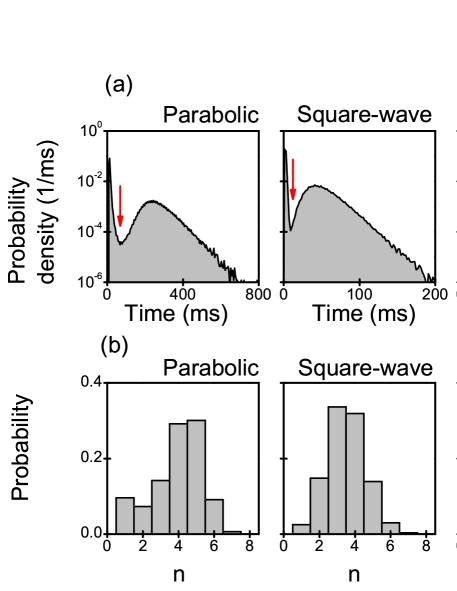
Figure 11: Statistical properties of bursting neurons. Example simulation of the minimal conductance-based models. Similar results are obtained with the normal forms, or the detailed conductance-based models. (a): ISI probability densities, with the local minimum defining the threshold ISI marked by arrows. Smaller ISIs correspond to intra-burst intervals, and longer ISIs, to inter-burst intervals. (b): Probability of finding a burst containing $n$ spikes, for different types of bursting neurons.

Stochastic stimulation

In all cases, the external current is given by Equation 2. There, $\xi(t)$ is an Ornstein-Uhlenbeck process of zero mean and unit variance, with a correlation time $\tau$. In Figures 4-6 and 8-10, the value of $I_{0}$ was chosen so that the average number of spikes per burst was approximately 3.5, and the value of $\sigma$ was chosen so that the standard deviation of the number of spikes per burst was approximately 1.5. The value of $\tau$ was chosen smaller than all the structure in the BTAs, but not as small as to require too extensive simulations in order to obtain smooth BTAs.

Model bursting neurons

For each type of bursting (parabolic, square-wave and elliptic), three neuron models are employed, with varying degree of biological detail. In all cases, with the parameters chosen for our simulations, a positive stimulus input was required in order to obtain bursting responses. If the stimulus was sufficiently high, burst firing was replaced by tonic activity.

Minimal normal-form models

These models were designed to represent the relevant bifurcation in their canonical form. The equations were taken from Izhikevich, (2007), except for the dynamics of the slow current in the elliptic case, here modified to stabilize the subthreshold behavior, since in the original model, the slow current diverges when the fast currents are quiescent.

The fast subsystem of parabolic and square-wave bursters is described by a single variable $V$ evolving with the dynamics of a quadratic integrate-and-fire model neuron. This model constitutes the canonical form of any type I neuron (Ermentrout and Kopell,, 1986). The equation is

$$\frac{{\rm d}V}{{\rm d}t}=V^{2}+\alpha I_{\rm burst}+I_{\rm ext},$$ (3)

where $I_{\rm burst}$ is the current produced by the slow subsystem as detailed below, and $I_{\rm ext}$ is the external current. The coupling constant $\alpha$ is varied in Figure 7, and set equal to unity in all other plots. There is a resetting rule supplementing Eq. 3, stating that whenever $V$ increases above $V_{\rm TH}$, it is discontinuously changed to a reset value $V_{R}$, and a spike is fired.

The fast subsystem of elliptic bursters involves two variables. The equations are usually given in radial coordinates $(r,\vartheta)$, such that the variable representing the voltage is $r\cos\vartheta$. The dynamics is governed by

$$\frac{{\rm d}r}{{\rm d}t} = I_{\rm burst}\ r+cr^{3}+dr^{5}$$

$$\frac{{\rm d}\vartheta}{{\rm d}t} = 1$$ (4)

The system of Eqs. 4 is the canonical form of a type II neuron with a subcritical bifurcation at firing onset (Brown et al.,, 2004). The external current $I_{\rm ext}$ is incorporated as an additive term in the equation for the voltage, obtained by transforming Eq. 4 to cartesian coordinates.

We now describe the dynamics of the slow subsystems. For parabolic bursters, $I_{\rm burst}=u_{1}-u_{2}$, where

$$\frac{{\rm d}u_{1}}{{\rm d}t} = -\mu_{1}u_{1}+d_{1}\delta(t-t_{\rm spike}),$$

$$\frac{{\rm d}u_{2}}{{\rm d}t} = -\mu_{2}u_{2}+d_{2}\delta(t-t_{\rm spike}),$$ (5)

where $t_{\rm spike}$ represents the time when the $V$ crosses the threshold voltage $V_{\rm TH}$ and generates a spike. At those times, the slow variables $u_{1}$ and $u_{2}$ are discontinuously reset to $u_{1}+d_{1}$ and $u_{2}+d_{2}$, respectively. For square-wave bursters, $I_{\rm burst}=-u_{1}$, where

$$\frac{{\rm d}u_{1}}{{\rm d}t}=-\mu_{1}u_{1}+d_{1}\delta(t-t_{\rm spike})$$ (6)

When $V$ crosses the threshold $V_{\rm TH}$, the slow variable $u_{1}$ is discontinuously changed to $u_{1}+d_{1}$. For elliptic bursters,

$$\frac{{\rm d}I_{\rm burst}}{{\rm d}t}=-\mu_{1}(I_{\rm burst}+\lambda r^{2})$$ (7)

In the case of elliptic bursting, no discontinuous resetting rule is used. Instead, a spike is fired whenever $r\cos\vartheta$ crosses the threshold 0.75. Table 1 specifies the parameters used in the simulations.

Parameter	Parabolic	Square-wave	Elliptic
	bursting	bursting	bursting
$I_{0}$	-0.1	-0.1	0
$\sigma$	0.25 ${\rm ms}^{1/2}$	1.4 ${\rm ms}^{1/2}$	0.75 ${\rm ms}^{1/2}$
$\tau$	1 ms	0.5 ms	0.2 ms
$V_{TH}$	20	10	-
$V_{\rm R}$	-1	1	-
$\mu_{1}$	0.1 ${\rm ms}^{-1}$	0.015 ${\rm ms}^{-1}$	0.0025 ${\rm ms}^{-1}$
$d_{1}$	1.1	0.22	-
$\mu_{2}$	0.02 ${\rm ms}^{-1}$	-	-
$d_{2}$	0.55	-	-
$\lambda$	-	-	1.25
$c$	-	-	0.4
$d$	-	-	-0.2
dt	0.1 ${\rm ms}$	0.05 ${\rm ms}$	0.01 ${\rm ms}$
$\alpha$	1	1	1

Table 1: Parameters of the minimal normal-form models used in Figs. 4-6 and 8-10. Figure 7 was built with the same parameters except for the coupling strength $\alpha$.

Minimal conductance-based models

These models are taken from Izhikevich, (2007). Spiking is induced by the fast subsystem, containing a fast persistent sodium current and a potassium current. Bursting is modulated by the slow subsystem, involving one or two additional slow variables. For all bursting types, the equations of the fast subsystem read

$$C\frac{{\rm d}V}{{\rm d}t} = -g_{\rm Na}\ m_{\infty}(V)\ (V-V_{\rm Na})-g_{\rm K}\ n\ (V-V_{\rm K})$$

$$-g_{\rm L}\ (V-V_{\rm L})+\alpha I_{\rm burst}+I_{\rm ext}$$

$$\frac{{\rm d}n}{{\rm d}t} = \left[n_{\infty}(V)-n\right]/\tau_{\rm n}.$$ (8)

In Figure 1, $\alpha$ takes the values 0.5, 1, and 1.1. Throughout the rest of the paper, $\alpha$ is maintained fixed at 1. The activation curves $x_{\infty}$ are

$$x_{\infty}(V)=\frac{1}{1+\exp\left[(V_{1/2}^{x}-V)/k^{x}\right]},$$ (9)

and the parameters depend on the type of bursting, as specified in Table 2. In the parabolic burster, the slow subsystem is described by two variables, associated with sodium and potassium currents, respectively. That is, the bursting current reads

$$I_{\rm burst}=-g_{{\rm ms}}m_{{\rm s}}(V-V_{{\rm Na}})-g_{{\rm ns}}n_{{\rm s}}(V-V_{{\rm K}}),$$ (10)

and

$$\frac{{\rm d}m_{\rm s}}{{\rm d}t} = \left[m_{{\rm s}\ \infty}(V)-m_{\rm s}\right]/\tau_{\rm ms},$$

$$\frac{{\rm d}n_{\rm s}}{{\rm d}t} = \left[n_{{\rm s}\ \infty}(V)-n_{\rm s}\right]/\tau_{\rm ns}.$$ (11)

In the square-wave and the elliptic bursters, the slow subsystem is described by a single variable, associated with a potassium current,

$$I_{\rm burst}=-g_{{\rm ns}}n_{{\rm s}}(V-V_{{\rm K}}),\ \$$ (12)

and $n_{\rm s}$ is governed by Eq. 11. Parameters are given in Table 2.

Parameter	Parabolic	Square-wave	Elliptic
	bursting	bursting	bursting
$I_{0}$	1.2 $\mu$A/cm2	4 $\mu$A/cm2	48 $\mu$A/cm2
$\sigma$	2 $\mu$A/cm2	2.75 $\mu$A/cm2	3 $\mu$A/cm2
$\tau$	1 ms	0.5 ms	1 ms
$C$	1 $\mu$F/cm2	1 $\mu$F/cm2	1 $\mu$F/cm2
$V_{\rm Na}$	60 mV	60 mV	60 mV
$V_{\rm K}$	-90 mV	-90 mV	-90 mV
$V_{\rm L}$	-80 mV	-80 mV	-80 mV
$g_{\rm Na}$	20 mS/cm2	20 mS/cm2	4 mS/cm2
$g_{\rm K}$	10 mS/cm2	9 mS/cm2	4mS/cm2
$g_{\rm L}$	8 mS/cm2	8 mS/cm2	1 mS/cm2
$V_{1/2}^{\rm m}$	-20 mV	-20 mV	-30 mV
$k^{\rm m}$	15 mV	15 mV	7 mV
$V_{1/2}^{\rm n}$	-25 mV	-25 mV	-45 mV
$k^{\rm n}$	5 mV	5 mV	5 mV
$\tau_{\rm n}$	1 ms	0.152 ms	1 ms
$g_{\rm ms}$	3 mS/cm2	-	-
$V_{1/2}^{\rm ms}$	-40 mV	-	-
$k^{\rm ms}$	5 mV	-	-
$\tau_{\rm ms}$	20 ms	-	-
$g_{\rm ns}$	20 mS/cm2	5 mS/cm2	1.5 mS/cm2
$V_{1/2}^{\rm ns}$	-20 mV	-20 mV	-20 mV
$k^{\rm ns}$	5 mV	5 mV	5 mV
$\tau_{\rm ns}$	50 ms	20 ms	60 ms

Table 2: Parameters of the minimal conductance-based models used in Figures 4-6 and 8-10. Figures 1-3 were constructed with the same parameters, except for $I_{0}$ and $\sigma$.

Detailed conductance-based models

The Chay-Cook model is a detailed conductance-based model of a pancreatic $\beta$-cell that can produce parabolic, square-wave or elliptic bursting, depending on the parameters (Chay and Cook,, 1988). The model includes two inward Ca²⁺ currents ($I_{{\rm I}}$ and $I_{{\rm S}}$), an outward delayed-rectifier Potassium current ($I_{{\rm K}}$), and a leakage current ($I_{{\rm L}}$).

$$C\frac{{\rm d}V}{{\rm d}t} = -I_{{\rm Ca}}(V,s)-I_{\rm K}(V,n)-I_{\rm L}(V)$$

$$\frac{{\rm d}n}{{\rm d}t} = \lambda\frac{n_{\infty}(V)-n}{\tau_{n}(V)}$$

$$\frac{{\rm d}s}{{\rm d}t} = \frac{s_{\infty}(V,c)-s}{\tau_{s}(V,c)}$$

$$\frac{{\rm d}c}{{\rm d}t} = f\left[-\alpha I_{{\rm Ca}}(V,s)-k_{\rm c}c\right]$$ (13)

where $V$ is the membrane potential, $c$ is the intracellular free Ca²⁺ concentration, $n$ and $s$ are the activation variables. The ionic currents are given by

$$I_{{\rm Ca}}(V,s) = I_{{\rm I}}(V)+I_{{\rm S}}(V,s)$$

$$I_{{\rm I}}(V) = g_{{\rm I}}\ m_{\infty}(V)\ \left(V-V_{{\rm Ca}}\right)$$

$$I_{{\rm S}}(V,s) = g_{{\rm S}}\ s\ \left(V-V_{{\rm Ca}}\right)$$

$$I_{{\rm K}}(V,n) = g_{{\rm K}}\ n\ \left(V-V_{{\rm K}}\right)$$

$$I_{{\rm L}}(V) = g_{{\rm L}}\ \left(V-V_{{\rm L}}\right)$$ (14)

The steady-state functions and activation times are

$$x_{\infty}(V) = \frac{1}{1+\exp\left[\left(V_{x}-V\right)/S_{x}\right]},\ \ \ {\rm for}\ x=m,n$$

$$s_{\infty}(V,c) = \frac{1}{1+\exp\left[2A(V,c)\right]},$$

$$\tau_{\rm n}(V) = \frac{\tau_{\rm n0}}{1+\exp\left[\left(V-V_{\rm n}\right)/S_{\rm n}\right]},$$

$$\tau_{\rm s}(V,c) = \frac{\tau_{\rm s0}}{2\cosh(A(V,c))},$$

$$A(V,c) = \frac{V_{{\rm s}}+S_{{\rm s}}\log(\tilde{c})-V}{2S_{{\rm s}}},$$ (15)

and $\tilde{c}=c/(1\mu{\rm M})$.

Parameter	Parabolic	Square-wave	Elliptic
	bursting	bursting	bursting
$I_{0}$	-50 $\mu$A/cm2	-100 $\mu$A/cm2	-50 $\mu$A/cm2
$\sigma$	50 $\mu$A/cm2	200 $\mu$A/cm2	60 $\mu$A/cm2
$\tau$	50 ms	50 ms	50 ms
$\tau_{n}^{0}$	9.09 ms	9.09 ms	9.09 ms
$\tau_{s}^{0}$	100 ms	0.1 ms	0.1 ms
$C$	4524 fF	4524 fF	1 4524 fF
$V_{\rm Ca}$	100 mV	100 mV	100 mV
$V_{\rm K}$	-80 mV	-80 mV	-80 mV
$V_{\rm L}$	-60 mV	-60 mV	-60 mV
$g_{\rm I}$	250 pS	250 pS	250 pS
$g_{\rm K}$	1300 pS	1300 pS	1300 pS
$g_{\rm L}$	50 pS	50 pS	50 pS
$g_{\rm S}$	10 pS	10 pS	10 pS
$V_{\rm m}$	-22 mV	-22 mV	-22 mV
$V_{\rm n}$	-9 mV	-9 mV	-9 mV
$V_{\rm s}$	-22 mV	-22 mV	-22 mV
$S_{\rm m}$	7.5 mV	7.5 mV	7.5 mV
$S_{\rm n}$	10 mV	10 mV	10 mV
$S_{\rm s}$	10 mV	10 mV	10 mV
$\alpha_{\rm n}$	5.727 $10^{-6}$ fA${}^{-1}\mu$M ms-1	5.727 $10^{-6}$ fA${}^{-1}\mu$M ms-1	5.727 $10^{-6}$ fA${}^{-1}\mu$M ms-1
$k_{\rm c}$	0.03 ms-1	0.027 ms-1	0.022 ms-1
$\lambda$	0.6	0.95	0.1
$f$	0.0015	0.002	0.002

Table 3: Parameters of the Chay-Cook model models used in Figures. 4-6 and 8-10.

Covariance analysis

In order to disclose the stimulus features responsible for burst generation, we use spike-triggered covariance techniques (Paninski,, 2003; Samengo and Gollisch,, 2013). We define $P_{n}[t_{0}|s(t)]$ as the probability of generating a burst of $n$ spikes at time $t_{0}$ conditional to a time-dependent stimulus $s(t)$. We assume that $P_{n}$ only depends on the stimulus $s(t)$ through a few relevant features $f^{1}(t-t_{0}),f^{2}(t-t_{0}),\dots f^{k}(t-t_{0})$. The stimulus and the relevant features are continuous functions of time. For computational purposes, we represent them as vectors ${\bf s}$ and ${\bf f}_{i}$ of $N$ components, where each component $s_{j}=s(j\ \delta t)$ and $f^{i}_{j}=f^{i}(j\ \delta t)$ is the value of the stimulus evaluated at discrete intervals $\delta t$. If $\delta t$ is small compared with the relevant timescales of the models, the discretized signal is still a good approximation of the original continuous function. The relevant features ${\bf f}^{1},\dots,{\bf f}^{k}$ lie in the space spanned by those eigenvectors of the matrix

$${\rm M}={\rm C_{p}}^{-1}\ {\rm C},$$ (16)

whose eigenvalues are significantly different from unity (Samengo and Gollisch,, 2013). Here, ${\rm C}$ is the $N\times N$ $n$-burst-triggered covariance matrix,

$$({\rm C})_{ij}=\frac{1}{N_{\rm n}-1}\sum_{t_{0}}s(t_{i}+t_{0})\ s(t_{j}+t_{0})-s_{0}(t_{i})\ s_{0}(t_{j}),$$

where the sum is taken over all the times $t_{0}$ where bursts of $n$ spikes are initiated, $N_{\rm n}$ is the total number of bursts witn $n$ spikes, and $s_{0}(t)$ is the n-burst-triggered average (BTA):

$$s_{0}(t)=\frac{1}{N_{\rm n}}\sum_{t_{0}}s(t+t_{0}).$$

In Equation 16$,{\rm C_{p}}$ is the $N\times N$ prior covariance matrix,

$$({\rm C_{p}})_{ij}=\overline{s(t_{i}+t)\ s(t_{j}+t)}-\left[\overline{s(t)}\right]^{2},$$

where the horizontal line represents a temporal average on the variable $t$.

The eigenvalues of $M$ that are larger than 1 correspond to directions in stimulus space where the stimulus segments associated with burst generation have an increased variance, as compared to the raw collection of stimulus segments. Such directions are often found in cells excited by stimuli that are large in modulus, and whose sign is irrelevant. Eigenvalues that lie significantly below unity are associated with stimulus directions of decreased variance. Such stimuli are often found in cells that respond to precisely tuned values of the stimulus. In general terms, the obtained eigenvalue is a measure of the ratio of variances of the two ensembles. That is, an eigenvalue that is noticeably smaller than unity indicates a certain feature for which the ratio of the variance of the burst-triggering stimuli and the variance of the raw stimuli is significantly small.

References

- Agmon and Connors, (1992) Agmon, A. and Connors, B. W. (1992). Correlation between intrinsic firing patterns and thalamocortical synaptic responses of neurons in mouse barrel cortex. The Journal of Neuroscience, 12(1):319–329.
- Alevizos et al., (1991) Alevizos, A., Skelton, M., Karagogeos, D., Weiss, K. R., and Koester, J. (1991). Possible role of bursting neuron r15 of aplysia in the control of egg-laying behavior. In Kits, K. S., Boer, H. H., and Joose, J., editors, Molluscan neurobiology, pages 61–66. North-Holland, Amsterdam.
- Arganda et al., (2007) Arganda, S., Guantes, R., and de Polavieja, G. G. (2007). Sodium pumps adapt spike bursting to stimulus statistics. Nature Neuroscience, 10(11):1467–73.
- Arnold, (2008) Arnold, V. I. (2008). Geometrical Methods in the Theory of Ordinary Differential Equations. Springer, Berlin-Heildelberg.
- Bertram et al., (1995) Bertram, R., Butte, M. J., Kiemel, T., and Sherman, A. (1995). Topological and phenomenological classification of bursting oscillations. Bulletin of Mathematical Biology, 57(3):413–39.
- Brown et al., (2004) Brown, E., Moehlis, J., and Holmes, P. (2004). On the phase reduction and response dynamics of neural oscillator populations. Neural Computation, 16(4):673–715.
- Cang and Isaacson, (2003) Cang, J. and Isaacson, J. S. (2003). In vivo whole-cell recording of odor-evoked synaptic transmission in the rat olfactory bulb. The Journal of Neuroscience, 23(10):4108–16.
- Chagnac Amitai and Connors, (1989) Chagnac Amitai, Y. and Connors, B. W. (1989). Synchronized excitation and inhibition driven by intrinsically bursting neurons in neocortex. Journal of Neurophysiology, 62(5):1149–62.
- Channell et al., (2009) Channell, P., Fuwape, I., Neiman, A., and Shilnikov, A. (2009). Variability of bursting patterns in a neuron model in the presence of noise. Journal of Computational Neuroscience, 27:527–542. 10.1007/s10827-009-0167-1.
- Chay and Cook, (1988) Chay, T. R. and Cook, D. L. (1988). Endogenous bursting patterns in excitable cells. Mathematical Biosciences, 90(1-2):139–153.
- DeBusk et al., (1997) DeBusk, B. C., DeBruyn, E. J., Snider, R. K., Kabara, J. F., and Bonds, A. B. (1997). Stimulus-dependent modulation of spike burst length in cat striate cortical cells. Journal of Neurophysiology, 78(1):199–213.
- Ermentrout and Kopell, (1986) Ermentrout, B. and Kopell, N. (1986). Parabolic bursting in an excitable system coupled with a slow oscillation. SIAM Journal on Applied Mathematics, 46:233–253.
- Eyherabide et al., (2008) Eyherabide, H. G., Rokem, A., Herz, A. V., and Samengo, I. (2008). Burst firing is a neural code in an insect auditory system. Frontiers in Computational Neuroscience, 2(0).
- Eyherabide et al., (2009) Eyherabide, H. G., Rokem, A., Herz, A. V., and Samengo, I. (2009). Bursts generate a non-reducible spike-pattern code. Frontiers in Neuroscience, 3(1):8–14.
- Gimbarzevsky et al., (1984) Gimbarzevsky, B., Miura, R. M., and Puil, E. (1984). Impedance profiles of peripheral and central neurons. Canadian journal of physiology and pharmacology, 62(4):460–2.
- Izhikevich, (2007) Izhikevich, E. M. (2007). Dynamical systems in neuroscience : the geometry of excitability and bursting. MIT Press, Cambridge, Mass.
- Izhikevich and Hoppensteadt, (2004) Izhikevich, E. M. and Hoppensteadt, F. C. (2004). Classification of bursting mappings. International Journal of Bifurcation and Chaos, 14:3847–3854.
- Kepecs et al., (2002) Kepecs, A., Wang, X. J., and Lisman, J. (2002). Bursting neurons signal input slope. The Journal of Neuroscience, 22(20):9053–62.
- Kuske and Baer, (2002) Kuske, R. and Baer, S. (2002). Asymptotic analysis of noise sensitivity in a neuronal burster. Bulletin of Mathematical Biology, 64:447–481. 10.1006/bulm.2002.0279.
- Marsat and Pollack, (2010) Marsat, G. and Pollack, G. S. (2010). The structure and size of sensory bursts encode stimulus information but only size affects behavior. Journal of comparative physiology. A, Neuroethology, sensory, neural, and behavioral physiology, 196(4):315–20.
- Martinez-Conde et al., (2002) Martinez-Conde, S., Macknik, S. L., and Hubel, D. H. (2002). The function of bursts of spikes during visual fixation in the awake primate lateral geniculate nucleus and primary visual cortex. Proceedings of the National Academy of Sciences of the United States of America, 99(21):13920–5.
- Mato and Samengo, (2008) Mato, G. and Samengo, I. (2008). Type i and type ii neuron models are selectively driven by differential stimulus features. Neural Computation, 20(10):2418–40.
- Meissner and Schmelz, (1974) Meissner, H. P. and Schmelz, H. (1974). Membrane potential of beta-cells in pancreatic islets. Pflugers Archiv : European journal of physiology, 351(3):195–206.
- Paninski, (2003) Paninski, L. (2003). Convergence properties of three spike-triggered analysis techniques. Network, 14(3):437–464.
- Pedersen and Sørensen, (2006) Pedersen, M. G. and Sørensen, M. P. (2006). The effect of noise on -cell burst period. SIAM Journal on Applied Mathematics, 67(2):pp. 530–542.
- Puil et al., (1986) Puil, E., Gimbarzevsky, B., and Miura, R. M. (1986). Quantification of membrane properties of trigeminal root ganglion neurons in guinea pigs. Journal of Neurophysiology, 55(5):995–1016.
- Rinzel, (1987) Rinzel, J. (1987). A formal classification of bursting mechanisms in excitable systems. In Teramoto, E. and Yamaguti, M., editors, Lecture Notes in Biomathematics, volume 71, pages 1578–1593. Springer-Verlag, Berlin.
- Samengo and Gollisch, (2013) Samengo, I. and Gollisch, T. (2013). Spike-triggered covariance: geometric proof, symmetry properties, and extension beyond gaussian stimuli. Journal of Computational Neuroscience, 34(1):137–161.
- Samengo and Montemurro, (2010) Samengo, I. and Montemurro, M. A. (2010). Conversion of phase information into a spike-count code by bursting neurons. PloS one, 5(3):e9669.
- Selverston and Miller, (1980) Selverston, A. I. and Miller, J. P. (1980). Mechanisms underlying pattern generation in lobster stomatogastric ganglion as determined by selective inactivation of identified neurons. i. pyloric system. Journal of Neurophysiology, 44(6):1102–21.
- Silva et al., (1991) Silva, L. R., Amitai, Y., and Connors, B. W. (1991). Intrinsic oscillations of neocortex generated by layer 5 pyramidal neurons. Science, 251(4992):432–5.
- Smith et al., (1991) Smith, J. C., Ellenberger, H. H., Ballanyi, K., Richter, D. W., and Feldman, J. L. (1991). Pre-botzinger complex: a brainstem region that may generate respiratory rhythm in mammals. Science, 254(5032):726–729.
- Steriade, (1991) Steriade, M. (1991). Alertness, quiet sleep, dreaming. In Peters, A., editor, Cerebral Cortex, volume 9, pages 279–357. Plenum, New York.
- Steriade et al., (1993) Steriade, M., McCormick, D. A., and Sejnowski, T. J. (1993). Thalamocortical oscillations in the sleeping and aroused brain. Science, 262(5134):679–85.
- Su et al., (2004) Su, J., Rubin, J., and Terman, D. (2004). Effects of noise on elliptic bursters. Nonlinearity, 17(1):133.