Diagonally Drift–Implicit Runge–Kutta Methods of Weak Order One and Two for Itô SDEs and Stability Analysis

Abstract

The class of stochastic Runge–Kutta methods for stochastic differential equations due to Rößler is considered. Coefficient families of diagonally drift–implicit stochastic Runge–Kutta (DDISRK) methods of weak order one and two are calculated. Their asymptotic stability as well as mean–square stability (MS–stability) properties are studied for a linear stochastic test equation with multiplicative noise. The stability functions for the DDISRK methods are determined and their domains of stability are compared to the corresponding domain of stability of the considered test equation. Stability regions are presented for various coefficients of the families of DDISRK methods in order to determine step size restrictions such that the numerical approximation reproduces the characteristics of the solution process.

and In honor of Professor Karl Strehmel

1 Introduction

Numerical methods are an important tool for the calculation of approximate solutions of stochastic differential equations (SDEs) which possess no analytical solution formula. Therefore, many approximation schemes have been developed in recent years and much research has been carried out to develop derivative free stochastic Runge–Kutta (SRK) type methods [2, 17, 18, 19, 27]. Similar to the well understood deterministic setting of ordinary differential equations (ODEs), one has to pay much attention to the stability properties of the solution as well as of the numerical approximations. Therefore, implicit methods have been proposed for the strong pathwise approximation of solutions of SDEs and their stability has been analyzed [2, 9, 16, 25]. However, for the approximation of moments of the solution process special numerical methods converging in the weak sense have to be applied (see, e.g., [11, 12, 13, 14, 17, 18, 19, 20, 21, 27]) and a stability analysis has to be carried out similar to that for strong approximations [9, 13, 26]. In the present paper, we present families of first and second order diagonally drift–implicit SRK (DDISRK) methods for the weak approximation of SDEs contained in the class of SRK methods proposed by Rößler [20]. Further, we analyze their asymptotic stability and mean–square stability for linear test equations with multiplicative noise. Finally, the regions of stability of the DDISRK methods are compared to the regions of stability of the linear test equation. Thus, in Section 2 we consider the class of SRK methods and coefficients families for weak order one and order two DDISRK methods are presented. Then, we discuss the concepts of stability for solutions of SDEs and for numerical approximations in Section 3 and Section 4, respectively. In Section 5, some numerical experiments are carried out in order to justify our theoretical results.

Let $(\Omega,\mathcal{F},\operatorname{P})$ be a probability space with a filtration $(\mathcal{F}_{t})_{t\geq 0}$ which fulfills the usual conditions and $\mathcal{I}=[t_{0},T]$ for some $0\leq t_{0}<T<\infty$. Then, let $X=(X_{t})_{t\in\mathcal{I}}$ denote the solution process of an Itô SDE

$${\mathrm{d}}X_{t}=a(t,X_{t})\,{\mathrm{d}}t+b(t,X_{t})\,{\mathrm{d}}W_{t},\qquad X_{t_{0}}=x_{0},$$ (1)

for $t\in\mathcal{I}$ where $a:\mathcal{I}\times\mathbb{R}^{d}\to\mathbb{R}^{d}$ is the drift and $b:\mathcal{I}\times\mathbb{R}^{d}\to\mathbb{R}^{d\times m}$ is the diffusion, $(W_{t})_{t\geq 0}$ is a $m$-dimensional Wiener process and a $\mathcal{F}_{t_{0}}$–measurable initial condition $x_{0}$ independent of $W_{t}-W_{t_{0}}$ for $t\geq t_{0}$ such that $\operatorname{E}(\|x_{0}\|^{2r})<\infty$ for some $r\in\mathbb{N}$. The $j$th column of the $d\times m$–diffusion matrix $b=(b^{ij})$ will be denoted by $b^{j}$ in the following. Further, we suppose that the conditions of the existence and uniqueness theorem [11] are fulfilled for SDE (1).

In the following, we consider time discrete approximations $Y^{h}=(Y_{t})_{t\in\mathcal{I}_{h}}$ w.r.t. a constant step size $h=\frac{T-t_{0}}{N}$ for some $N\in\mathbb{N}$ and $\mathcal{I}_{h}=\{t_{0},t_{1},\ldots,t_{N}\}$ where $t_{n}=t_{0}+n\,h$ for $0\leq n\leq N$. As usual, we also write $Y_{n}=Y_{t_{n}}$ for $0\leq n\leq N$. Further, let $C_{P}^{l}(\mathbb{R}^{d},\mathbb{R})$ denote the space of all $g\in C^{l}(\mathbb{R}^{d},\mathbb{R})$ fulfilling a polynomial growth condition [11].

Definition 1.1

A time discrete approximation $Y^{h}$ converges weakly with order $p>0$ to $X$ as $h\rightarrow 0$ at time $t\in\mathcal{I}_{h}$ if for each $f\in C_{P}^{2(p+1)}(\mathbb{R}^{d},\mathbb{R})$ exists a constant $C_{f}$, which does not depend on $h$, and a finite $\delta_{0}>0$ such that for each $h\in\,]0,\delta_{0}[\,$

$$|\operatorname{E}(f(X_{t}))-\operatorname{E}(f(Y_{t}))|\leq C_{f}\,h^{p}\,.$$ (2)

2 Diagonally Drift-Implicit Stochastic Runge–Kutta Methods

For the weak approximation of the solution of the Itô SDE (1), we consider the class of SRK methods introduced by Rößler [20]. Then, the $d$-dimensional approximation process $Y^{h}$ with $Y_{n}=Y_{t_{n}}$ for $t_{n}\in\mathcal{I}_{h}$ is given by the following SRK method of $s$-stages with $Y_{0}=x_{0}$ and

$$\begin{split}Y_{n+1}=Y_{n}&+\sum_{i=1}^{s}\alpha_{i}\,a(t_{n}+c_{i}^{(0)}h_{n},H_{i}^{(0)})\,h_{n}\\ &+\sum_{i=1}^{s}\sum_{k=1}^{m}\big{(}{\beta_{i}^{(1)}}\,\hat{I}_{(k),n}+{\beta_{i}^{(2)}}\,\frac{\hat{I}_{(k,k),n}}{\sqrt{h_{n}}}\big{)}\,b^{k}(t_{n}+c_{i}^{(1)}h_{n},H_{i}^{(k)})\\ &+\sum_{i=1}^{s}\sum_{k=1}^{m}\big{(}{\beta_{i}^{(3)}}\,\hat{I}_{(k),n}+{\beta_{i}^{(4)}}\,\sqrt{h_{n}}\big{)}\,b^{k}(t_{n}+{c}_{i}^{(2)}h_{n},\hat{H}_{i}^{(k)})\end{split}$$ (3)

for $n=0,1,\ldots,N-1$ with stage values

$$H_{i}^{(0)} =Y_{n} +\sum_{j=1}^{s}A_{ij}^{(0)}\,a(t_{n}+c_{j}^{(0)}h_{n},H_{j}^{(0)})\,h_{n}$$

$$+\sum_{j=1}^{s}\sum_{l=1}^{m}{B_{ij}^{(0)}}\,b^{l}(t_{n}+c_{j}^{(1)}h_{n},H_{j}^{(l)})\,\hat{I}_{(l),n}$$

$$H_{i}^{(k)} =Y_{n} +\sum_{j=1}^{s}A_{ij}^{(1)}\,a(t_{n}+c_{j}^{(0)}h_{n},H_{j}^{(0)})\,h_{n}$$

$$+\sum_{j=1}^{s}{B_{ij}^{(1)}}\,b^{k}(t_{n}+c_{j}^{(1)}h_{n},H_{j}^{(k)})\,\sqrt{h_{n}}$$

$$\hat{H}_{i}^{(k)} =Y_{n} +\sum_{j=1}^{s}{A}_{ij}^{(2)}\,a(t_{n}+c_{j}^{(0)}h_{n},H_{j}^{(0)})\,h_{n}$$

$$+\sum_{j=1}^{s}\sum_{\begin{subarray}{c}l=1\\ l\neq k\end{subarray}}^{m}{{B}_{ij}^{(2)}}\,b^{l}(t_{n}+c_{j}^{(1)}h_{n},H_{j}^{(l)})\,\frac{\hat{I}_{(k,l),n}}{\sqrt{h_{n}}}$$

for $i=1,\ldots,s$ and $k=1,\ldots,m$. The random variables of the method are defined by

$$\hat{I}_{(k,l),n}=\begin{cases}\tfrac{1}{2}(\hat{I}_{(k),n}\hat{I}_{(l),n}-\sqrt{h_{n}}\tilde{I}_{(k),n})&\text{if }k<l\\ \tfrac{1}{2}(\hat{I}_{(k),n}\hat{I}_{(l),n}+\sqrt{h_{n}}\tilde{I}_{(l),n})&\text{if }l<k\\ \tfrac{1}{2}(\hat{I}_{(k),n}^{2}-h_{n})&\text{if }k=l\end{cases}$$ (4)

for $1\leq k,l\leq m$ with independent random variables $\hat{I}_{(k),n}$ for $1\leq k\leq m$ and $\tilde{I}_{(k),n}$ for $1\leq k\leq m-1$ and $0\leq n<N$. Thus, only $2m-1$ independent random variables have to be simulated for each step. In the following, we choose $\hat{I}_{(k),n}$ as a three point distributed random variable with $\operatorname{P}(\hat{I}_{(k),n}=\pm\sqrt{3\,h_{n}})=\frac{1}{6}$ and $\operatorname{P}(\hat{I}_{(k),n}=0)=\frac{2}{3}$. The random variables $\tilde{I}_{(k),n}$ are defined by a two point distribution with $\operatorname{P}(\tilde{I}_{(k),n}=\pm\sqrt{h})=\tfrac{1}{2}$.

The main advantage of this class of SRK methods is the significant reduction of complexity compared to present SRK methods in recent literature, because the number of stages does not depend on the dimension $m$ of the driving Wiener process [20]. We denote by $\alpha=(\alpha_{i})$ and $\beta^{(k)}=(\beta^{(k)}_{i})$ for $1\leq k\leq 4$ the corresponding vectors of weights and by $A^{(k)}=(A^{(k)}_{ij})$ and $B^{(k)}=(B^{(k)}_{ij})$ for $k=0,1,2$ the corresponding coefficients matrices. Then, the coefficients of the SRK method (3) can be represented by an extended Butcher array:

$$c^{(0)}$$

Weak order one and two conditions for the SRK method (3) have been calculated in [20] by applying the colored rooted tree theory due to Rößler introduced in [17]. Now, let $p_{S}=p$ denote the order of convergence of the SRK method (3) if it is applied to an SDE and let $p_{D}$ with $p_{D}\geq p_{S}$ denote the order of convergence if it is applied to a deterministic ODE, i.e., SDE (1) with $b\equiv 0$ and we also write $(p_{D},p_{S})$ [17, 18]. Since we are interested in SRK methods which inherit good stability properties, we consider families of DDISRK methods which are diagonally implicit in the deterministic part of the scheme.

2.1 Weak Order One DDISRK Methods

Firstly, we consider weak order one DDISRK methods (3) with $s=1$ stage [20]. However, in order to cover the stochastic theta method [9, 11], we also consider the case that the stage number is $s=2$ for the drift function only, whereas it is still one for the diffusion function. Then, from the order conditions [20] it follows that the family of weak order one DDISRK methods is characterized by the Butcher table (5)

$$c_{1}$$ 0 0 0

0

0 0 0 0 0

0 0 0 0 0

0 0 0 0 0

0 0 0 0 0

0 0 0

0 0 0 0

(5)

with some coefficients $c_{1},c_{2},c_{3},c_{4},c_{5}\in\mathbb{R}$. As an example, in the case of $s=1$ stage we obtain for $c_{1}=c_{2}=c_{3}=c_{4}=c_{5}=0$ the explicit Euler-Maruyama scheme of order $(1,1)$ [11]. For $c_{1}=\frac{1}{2}$ and $c_{2}=c_{3}=c_{4}=c_{5}=0$ we obtain the SRK scheme DDIRDI1 with $s=1$ stage of order $(2,1)$, which reduces to the midpoint rule if it is applied to an ODE [5]. If we consider the case of $s=2$ stages, then we get for $c_{1}=0$, $c_{2}=1-\theta$, $c_{3}=\theta$, $c_{4}=1$ and $c_{5}=\theta$ for some $\theta\in[0,1]$ the SRK scheme DDIRDI2 of order $(2,1)$ which coincides with the stochastic theta method [9, 11, 23, 24]. Further, for $s=2$ stages with $c_{1}=c_{3}=\frac{3+\sqrt{3}}{6}$, $c_{2}=-\frac{1}{\sqrt{3}}$, $c_{5}=\frac{1}{2}$ and $c_{4}\in\mathbb{R}$ we get DDISRK schemes of order $(3,1)$ which are A-stable in case of ODEs [5]. Especially, in the case of $c_{4}=\frac{3}{2}$ we denote the scheme as DDIRDI3 in the following. Note that the schemes DDIRDI1 and DDIRDI2 for $\theta=\frac{1}{2}$ are also A-stable if they are applied to ODEs [5].

2.2 Weak Order Two DDISRK Methods

Next, we consider weak second order DDISRK methods (3) with $s=3$ stages. Here, we claim that $\alpha_{3}=0$ and $A^{(2)}_{ij}=0$ for $1\leq i,j\leq 3$ in order to reduce the computational effort. Since in this case the third stage $H^{(0)}_{3}$ does not matter anymore, we let $A^{(0)}_{3j}=B^{(0)}_{3j}=0$ for $1\leq j\leq 3$. Then, we can obtain $\alpha_{1}=\alpha_{2}=\frac{1}{2}$ from some order conditions of weak order two [20] and from the classification given in [4] in the case of an explicit SRK scheme. On the other hand, since we assume $A^{(2)}\equiv 0$, all conditions for $A^{(0)}$ to satisfy are $\alpha^{T}A^{(0)}e=\frac{1}{2}$ only. Therefore, we can consider arbitrary coefficients $A^{(0)}_{ij}$ as long as $\alpha^{T}A^{(0)}e=\frac{1}{2}$ is fulfilled for $\alpha_{1}=\alpha_{2}=\frac{1}{2}$. As a result of this, the weak order two DDISRK schemes (3) are given by the infinite coefficients family (6)

$$c_{1}$$ 0 0 0 0 0

0 1 0 0

0 0 0 0 0 0 0

0 0 0 0 0 0 0

0 0 0 0

0 0 0 0

0 0 0 0 0 0 0

0 0 0 0 0 0

0 0 0 0 0 0

0 0

0

(6)

with $c_{1},c_{2}\in\mathbb{R}$ and $c_{3},c_{4}\in\mathbb{R}\setminus\{0\}$. Clearly, one has to solve 2 (in general nonlinear) systems of equations from the stage values, each of dimension $d$, for the DDISRK method if $c_{1}\neq 0$ and $c_{2}\neq 0$. Therefore, as in the deterministic setting, some simplified Newton iterations have to be performed in each step in order to solve the nonlinear system of equations [3, 5]. As an example, for $c_{1}=c_{2}=\frac{3+\sqrt{3}}{6}$ and for all $c_{3},c_{4}\in\mathbb{R}\setminus\{0\}$ we obtain an DDISRK scheme of order $(3,2)$ which is A-stable if it is applied to a deterministic ODE [5].

3 Stability analysis for SDEs

For SDEs several stochastic stability concepts have been proposed in literature, see e.g., [9, 10, 11, 13, 15, 22, 23, 24, 26] and the literature therein. In the following, we consider SDE (1) with a steady solution $X_{t}\equiv 0$ such that $a(t,0)=b(t,0)=0$ holds, which is also called an equilibrium position. Suppose that there exists a unique solution $X_{t}=X(t;t_{0},x_{0})$ for all $t\geq t_{0}$ and for each nonrandom initial value $x_{0}$ under consideration. Then, stochastic stability can be defined as the stochastic counterparts of stability, asymptotic stability and asymptotic stability in the large for ODEs [1, 6, 11].

Definition 3.1

Let $X$ be the solution of the scalar Itô SDE (1). Then, the equilibrium position of the SDE is said to be

1. stochastically stable if for all $\epsilon>0$ and $t_{0}\geq 0$ holds

   $$\lim_{x_{0}\to 0}\operatorname{P}\left(\sup_{t\geq t_{0}}|X(t;t_{0},x_{0})|\geq\epsilon\right)=0\,,$$

2. stochastically asymptotically stable if (i) holds and if

   $$\lim_{x_{0}\to 0}\operatorname{P}\left(\lim_{t\to\infty}|X(t;t_{0},x_{0})|=0\right)=1\,,$$

3. or stochastically asymptotically stable in the large if (i) holds and if for all $x_{0}\in\mathbb{R}$ holds

   $$\operatorname{P}\left(\lim_{t\to\infty}|X(t;t_{0},x_{0})|=0\right)=1\,.$$

Further, stability analysis involving the $p$th moments of the solution process is also widely considered, see e.g. [1, 9, 10, 11, 13].

Definition 3.2

Let $X$ be the solution of the scalar Itô SDE (1). Then, the equilibrium position of the SDE is said to be

1. stable in the $p$th–mean if for every $\epsilon>0$ and $t_{0}\geq 0$ there exists a $\delta=\delta(t_{0},\epsilon)>0$ such that for all $t\geq t_{0}$ and $|x_{0}|<\delta$

   $$\operatorname{E}\left(|X(t;t_{0},x_{0})|^{p}\right)<\epsilon\,,$$

2. asymptotically stable in the $p$th–mean if (i) holds and if there exists a $\delta_{0}=\delta_{0}(t_{0})>0$ such that for all $|x_{0}|<\delta_{0}$

   $$\lim_{t\to\infty}\operatorname{E}\left(|X(t;t_{0},x_{0})|^{p}\right)=0\,.$$

The most frequently used cases in applications are $p=1$ and $p=2$, i.e., stability in mean (M-stability) and mean–square stability (MS-stability). In the present paper, we will focus on asymptotic stability in the large and MS-stability for a linear test equation with multiplicative noise [8, 9, 10, 23]

$${\mathrm{d}}X_{t}=\lambda\,X_{t}\,{\mathrm{d}}t+\mu\,X_{t}\,{\mathrm{d}}W_{t}$$ (7)

for $t\geq t_{0}$ and with some constants $\lambda,\mu\in\mathbb{C}$ and with a nonrandom initial condition $X_{t_{0}}=x_{0}\in\mathbb{R}\setminus\{0\}$, which reproduces the dynamics of more complex SDEs better than in the case of additive noise [7, 11]. The exact solution of (7) can be calculated as $X_{t}=x_{0}\,\exp((\lambda-\tfrac{1}{2}\mu^{2})(t-t_{0})+\mu(W_{t}-W_{t_{0}}))$ which is stochastically asymptotically stable in the large [23] if

$$\begin{split}\lim_{t\to\infty}|X_{t}|=0\text{ with probability 1}\quad&\Leftrightarrow\quad\Re(\lambda-\tfrac{1}{2}\mu^{2})<0\,.\end{split}$$ (8)

We calculate that $|X_{t}|^{p}=|x_{0}|^{p}\,\exp(p\,\Re(\lambda-\tfrac{1}{2}\mu^{2})(t-t_{0})+p\,\Re(\mu)(W_{t}-W_{t_{0}}))$ which yields $\operatorname{E}(|X_{t}|^{p})=|x_{0}|^{p}\,\exp(p\,\Re(\lambda-\tfrac{1}{2}\mu^{2})(t-t_{0})+\tfrac{1}{2}p^{2}(\Re(\mu))^{2}(t-t_{0}))$. Then the $p$th–mean stability domain where SDE (7) possesses an equilibrium position can be determined as follows:

$$\lim_{t\to\infty}\operatorname{E}(|X_{t}|^{p})=0\quad\Leftrightarrow\quad 2\,\Re(\lambda)-\Re(\mu^{2})+p\,(\Re(\mu))^{2}<0\,.$$ (9)

Thus, the equilibrium position of SDE (7) is asymptotically MS–stable if

$$\lim_{t\to\infty}\operatorname{E}(|X_{t}|^{2})=0\quad\Leftrightarrow\quad 2\,\Re(\lambda)+|\mu|^{2}<0$$ (10)

for the coefficients $\lambda,\mu\in\mathbb{C}$ (see, e.g., [9, 23, 26]). We remark that due to $\Re(2\lambda-\mu^{2})\leq 2\,\Re(\lambda)+|\mu|^{2}$ MS-stability always induces asymptotically stability in the large. Further, for $\mu=0$ the stability condition (9) reduces to the well known deterministic stability condition $\Re(\lambda)<0$.

4 Numerical stability of SRK methods

We are now looking for conditions such that a numerical method applied to SDE (7) yields numerically stable solutions. Therefore, we say that the method is numerically asymptotically stable or MS–stable if the numerical solutions $Y_{n}$ satisfy $\lim_{n\to\infty}|Y_{n}|=0$ with probability one or $\lim_{n\to\infty}\operatorname{E}\left(|Y_{n}|^{2}\right)=0$, respectively. If we apply the numerical method to the linear test equation (7), then we obtain with the parametrization $\hat{h}=\lambda\,h$ and $k=\mu\sqrt{h}$ [9, 13] a one–step difference equation of the form

$$Y_{n+1}=R_{n}(\hat{h},k)\,Y_{n}=\prod_{i=0}^{n}R_{i}(\hat{h},k)\,Y_{0}\,.$$ (11)

with a stability function $R_{n}(\hat{h},k)$. The domain of asymptotic stability of a numerical method can be determined by the following lemma [9]:

Lemma 4.1

Given a sequence of real-valued, non-negative, independent and identically distributed random variables $(|R_{n}(\hat{h},k)|)_{n\in\mathbb{N}_{0}}$, consider the sequence of random variables $(|Y_{n}|)_{n\in\mathbb{N}_{0}}$ defined by (11) where $|Y_{0}|\neq 0$ with probability 1. Suppose that the random variables $\log(R_{n}(\hat{h},k))$ are square-integrable. Then

$$\lim_{n\to\infty}|Y_{n}|=0\,,\text{ with probability 1 }\Leftrightarrow\,\operatorname{E}(\log(R_{n}(\hat{h},k)))<0\,.$$ (12)

We call the set $\mathcal{R}_{AS}=\{(\hat{h},k)\in\mathbb{C}^{2}:\operatorname{E}(\log(R_{n}(\hat{h},k)))<0\}\subset\mathbb{C}^{2}$ the domain of asymptotical stability of the method. Note that one can also find some alternative parameterizations like $k=-\frac{\mu^{2}}{\lambda}$ in the literature [1, 23, 26]. Analogously, if we calculate the mean–square norm $z_{n}=\operatorname{E}(|Y_{n}|^{2})$ then we obtain a one–step difference equation of the form $z_{n+1}=\hat{R}(\hat{h},k)\,z_{n}$ where $\hat{R}(\hat{h},k)=\operatorname{E}(|R_{n}(\hat{h},k)|^{2})$ is called the MS–stability function of the numerical method. Thus, we obviously yield MS–stability, i.e. $z_{n}\to 0$ as $n\to\infty$, if $\hat{R}(\hat{h},k)<1$. The set $\mathcal{R}_{MS}=\{(\hat{h},k)\in\mathbb{C}^{2}:\hat{R}(\hat{h},k)<1\}\subset\mathbb{C}^{2}$ is called the domain of MS–stability of the method.

Especially, the domain is called region of stability in the case of $(\hat{h},k)\in\mathbb{R}^{2}$ [23]. The numerical method is said to be $A$–stable if the domain of stability of the test equation (7) is a subset of the domain of numerical stability. Since the domain of stability for $\lambda,\mu\in\mathbb{C}$ is not easy to visualize, we restrict our attention to figures presenting the region of stability with $\lambda,\mu\in\mathbb{R}$ in the $\hat{h}$–$k^{2}$ plane. Then, for fixed values of $\lambda$ and $\mu$, the set $\{(\lambda\,h,\mu^{2}\,h)\subset\mathbb{R}^{2}:h>0\}$ is a straight ray starting at the origin and going through the point $(\lambda,\mu^{2})$. Clearly, varying the step size $h$ corresponds to moving along this ray. For $\lambda,\mu\in\mathbb{R}$, the region of asymptotical stability for SDE (7) reduces to the area of the $\hat{h}$–$k^{2}$ plane with the $\hat{h}$–axis as the lower bound if $\hat{h}<0$ and with $k^{2}>2\hat{h}$ as the lower bound if $\hat{h}\geq 0$ whereas the region of MS–stability for SDE (7) reduces to the area of the $\hat{h}$–$k^{2}$ plane with the $\hat{h}$–axis as the lower bound and $k^{2}<-2\hat{h}$ as the upper bound for $\hat{h}<0$.

In the following, all figures presenting regions of stability for some numerical method under consideration are plotted by the software Mathematica. The regions of numerical asymptotically stability and MS–stability are indicated by two dark–grey tones whereas the regions of MS–stability are more dark than the regions of asymptotical stability. Further, the corresponding regions of stability for the test equation (7) are filled by two light–grey tones whereas again the regions of MS–stability are more dark than the regions of asymptotical stability. In all presented figures, the regions of MS–stability are a subset of the regions of asymptotical stability.

4.1 Stability of Order One DDISRK Schemes

We consider the family of order one DDISRK schemes (5) with coefficients $c_{1},\ldots,c_{5}\in\mathbb{R}$. If we apply these schemes to the linear test equation (7) then we obtain the difference equation

$$Y_{n+1}=Y_{n}+(1-c_{5})\,\lambda\,h\,H_{1}^{(0)}+c_{5}\,\lambda\,h\,H_{2}^{(0)}+\mu\,\hat{I}_{(1),n}\,H^{(1)}_{1}$$ (13)

with the stage values

$$\begin{split}H^{(0)}_{1}&=Y_{n}+c_{1}\,\lambda\,h\,H^{(0)}_{1}\\ H^{(0)}_{2}&=Y_{n}+c_{2}\,\lambda\,h\,H^{(0)}_{1}+c_{3}\,\lambda\,h\,H^{(0)}_{2}+c_{4}\,\mu\,\hat{I}_{(1),n}\,H^{(1)}_{1}\\ H^{(1)}_{1}&=Y_{n}\end{split}$$ (14)

where the implicit equations for $H^{(0)}_{1}$ and $H^{(0)}_{2}$ can be solved in the case of $1-c_{1}\,\lambda\,h\neq 0$ and $1-c_{3}\,\lambda\,h\neq 0$, which is fulfilled for step sizes $h\neq\frac{1}{c_{1}\,\lambda}$ if $c_{1}\neq 0$ and $h\neq\frac{1}{c_{3}\,\lambda}$ if $c_{3}\neq 0$. With $\hat{h}=\lambda\,h$ and $k=\mu\sqrt{h}$ let

$$\begin{split}&\Gamma=1+\frac{\hat{h}-c_{3}\,\hat{h}^{2}+c_{5}\,(c_{2}+c_{3}-c_{1})\,\hat{h}^{2}}{(1-c_{1}\,\hat{h})(1-c_{3}\,\hat{h})}\,,\qquad\Sigma=\frac{c_{4}\,c_{5}\,\hat{h}}{1-c_{3}\,\hat{h}}\,k+k\,.\end{split}$$

Then, we can write (13) by the recursion formula $Y_{n+1}=R_{n}(\hat{h},k)\,Y_{n}$ with the stability function $R_{n}(\hat{h},k)=\Gamma+h^{-1/2}\,\Sigma\,\hat{I}_{(1),n}$ for $n=0,\ldots,N-1$. Since the SRK schemes (5) are of weak order one, we can substitute the tree point distributed random variables $\hat{I}_{(j),n}$ by two point distributed random variables $\tilde{I}_{(j),n}$ for $1\leq j\leq m$ in (3) and consider $R_{n}(\hat{h},k)=\Gamma+h^{-1/2}\,\Sigma\,\tilde{I}_{(1),n}$ instead. Now, we analyse the asymptotic stability of the SRK schemes (5) by applying Lemma 4.1. Further, in order to analyse the MS-stability, we calculate the mean–square norm $z_{n}=\operatorname{E}(|Y_{n}|^{2})$. Then, we obtain the recursion formula $z_{n+1}=\hat{R}(\hat{h},k)\,z_{n}$ with the MS–stability function $\hat{R}(\hat{h},k)=|\Gamma|^{2}+|\Sigma|^{2}$.

Proposition 4.2

For SDE (7) with $\lambda,\mu\in\mathbb{C}$, the SRK schemes (5) are

1. numerically asymptotical stable if $|\Gamma^{2}-3\,\Sigma^{2}|\,|\Gamma|^{4}<1$ and in the case that the random variables $\hat{I}_{(j),n}$ are replaced by $\tilde{I}_{(j),n}$ for $1\leq j\leq m$, if $|\Gamma^{2}-\Sigma^{2}|<1$,

2. numerically MS–stable if $|\Gamma|^{2}+|\Sigma|^{2}<1$.

Here, we have to point out that the distribution of the random variables used for the numerical method has significant influence on the domain of asymptotical stability. As an example, for DDIRDI1 we have $\Gamma=\frac{1+\frac{1}{2}\hat{h}}{1-\frac{1}{2}\hat{h}}$, $\Sigma=k$ and we calculate $\mathcal{R}_{AS}=\{(\hat{h},k)\in\mathbb{C}^{2}:|(1+\frac{1}{2}\hat{h})^{2}-(1-\frac{1}{2}\hat{h})^{2}k^{2}|<|1-\frac{1}{2}\hat{h}|^{2}\}$ if the random variables $\tilde{I}_{(j),n}$ are used and $\mathcal{R}_{AS}=\{(\hat{h},k)\in\mathbb{C}^{2}:|(1-\frac{1}{2}\hat{h})^{2}(1+\frac{1}{2}\hat{h})^{2}(1-3k^{2})||1+\frac{1}{2}\hat{h}|^{4}<|1-\frac{1}{2}\hat{h}|^{4}\}$ if $\hat{I}_{(j),n}$ are used. In both cases, we get $\mathcal{R}_{MS}=\{(\hat{h},k)\in\mathbb{C}^{2}:2\Re(\hat{h})+((1-\frac{1}{2}\Re(\hat{h}))^{2}+\frac{1}{4}(\Im(\hat{h}))^{2})\,|k|^{2}<0\}$. The corresponding regions of stability are presented for both cases in Figure 1. For DDIRDI2 we get $\Gamma=\frac{1+(1-\theta)\hat{h}}{1-\theta\hat{h}}$ and $\Sigma=\frac{\theta\hat{h}}{1-\theta\hat{h}}k+k$, $\theta\in[0,1]$. Then, for $\theta=\frac{1}{2}$ follows $\mathcal{R}_{AS}=\{(\hat{h},k)\in\mathbb{C}^{2}:|(1+\frac{1}{2}\hat{h})^{2}-k^{2}|<|1-\frac{1}{2}\hat{h}|^{2}\}$ if $\tilde{I}_{(j),n}$ are used, $\mathcal{R}_{AS}=\{(\hat{h},k)\in\mathbb{C}^{2}:|(1-\frac{1}{2}\hat{h})^{2}((1+\frac{1}{2}\hat{h})^{2}-3k^{2})||1+\frac{1}{2}\hat{h}|^{4}<|1-\frac{1}{2}\hat{h}|^{4}\}$ if $\hat{I}_{(j),n}$ are used and $\mathcal{R}_{MS}=\{(\hat{h},k)\in\mathbb{C}^{2}:2\Re(\hat{h})+|k|^{2}<0\}$. Thus, the scheme DDIRDI2 with $\theta=\frac{1}{2}$ is $A$–stable w.r.t. MS–stability and the corresponding regions are presented in Figure 2 (see also [9, 23]). Analogously, we can calculate the domains of stability for DDIRDI3 which are presented in Figure 3. For all considered schemes, we can see the influence of the random variables used by the scheme to the domain of asymptotical stability.

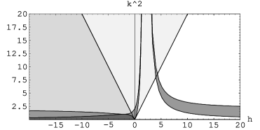
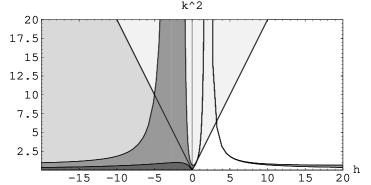
Figure 1: Asymptotical and mean–square stability region for DDIRDI1 with two point and three point distributed random variables in the left and right figure, respectively.

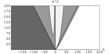
Figure 2: Asymptotical and mean–square stability region for DDIRDI2 with two point and three point distributed random variables in the left and right figure, respectively.

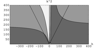
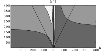
Figure 3: Asymptotical and mean–square stability region for DDIRDI3 with two point and three point distributed random variables in the left and right figure, respectively.

4.2 Stability of Order Two DDISRK Schemes

Next, we apply the DDISRK method (3) with the coefficients (6) to the linear test equation (7). Then we obtain the difference equation

$$\begin{split}Y_{n+1}=\,\,&Y_{n}+\frac{1}{2}\,\lambda\,h\,H_{1}^{(0)}+\frac{1}{2}\,\lambda\,h\,H_{2}^{(0)}\\ &+\left(1-\frac{1}{2c_{3}^{2}}\right)\,\mu\,\hat{I}_{(1)}\,H_{1}^{(1)}+\frac{1}{4c_{3}^{2}}\,\mu\,\hat{I}_{(1)}\,H_{2}^{(1)}+\frac{1}{4c_{3}^{2}}\,\mu\,\hat{I}_{(1)}\,H_{3}^{(1)}\\ &+\frac{1}{2c_{3}}\,\mu\,\frac{\hat{I}_{(1,1)}}{\sqrt{h}}\,H_{2}^{(1)}-\frac{1}{2c_{3}}\,\mu\,\frac{\hat{I}_{(1,1)}}{\sqrt{h}}\,H_{3}^{(1)}\end{split}$$ (15)

with stage values

$$\begin{split}H_{1}^{(0)}&=Y_{n}+c_{1}\,\lambda\,h\,H_{1}^{(0)}\\ H_{2}^{(0)}&=Y_{n}+(1-c_{1}-c_{2})\,\lambda\,h\,H_{1}^{(0)}+c_{2}\,\lambda\,h\,H_{2}^{(0)}+\mu\,\hat{I}_{(1)}\,H_{1}^{(1)}\\ H_{1}^{(1)}&=Y_{n}\\ H_{2}^{(1)}&=Y_{n}+c_{3}^{2}\,\lambda\,h\,H_{1}^{(0)}+c_{3}\,\mu\,\sqrt{h}\,H_{1}^{(1)}\\ H_{3}^{(1)}&=Y_{n}+c_{3}^{2}\,\lambda\,h\,H_{1}^{(0)}-c_{3}\,\mu\,\sqrt{h}\,H_{1}^{(1)}\end{split}$$ (16)

where the values $\hat{H}^{(1)}_{i}$ do not appear due to $m=1$ and $A^{(2)}\equiv 0$. Suppose that $1-c_{1}\,\lambda\,h\neq 0$ and that $1-c_{2}\,\lambda\,h\neq 0$ which can always be fulfilled for step sizes $h$ with $h\neq\frac{1}{c_{1}\,\lambda}$ and $h\neq\frac{1}{c_{2}\,\lambda}$. Then the implicit equations for $H_{1}^{(0)}$ and $H_{2}^{(0)}$ can always be solved. Let with $\hat{h}=\lambda\,h$ and $k=\mu\sqrt{h}$

$$\begin{split}\Gamma&=1+\frac{\hat{h}+(\frac{1}{2}-c_{1}-c_{2})\hat{h}^{2}}{(1-c_{1}\,\hat{h})(1-c_{2}\,\hat{h})}\,,\quad\Sigma=\frac{\hat{h}-\frac{1}{2}(c_{1}+c_{2})\hat{h}^{2}}{(1-c_{1}\,\hat{h})(1-c_{2}\,\hat{h})}\,k+k\,,\quad\Lambda=\frac{1}{2}k^{2}\,.\end{split}$$

Then, we yield for (15) the recursion formula $Y_{n+1}=R_{n}(\hat{h},k)\,Y_{n}$ with the stability function $R_{n}(\hat{h},k)=\Gamma-\Lambda+h^{-1/2}\,\Sigma\,\hat{I}_{(1),n}+h^{-1}\,\Lambda\,\hat{I}_{(1),n}^{2}$. In order to analyse the asymptotic stability of the weak order two DDISRK schemes (6) we apply again Lemma 4.1. For the determination of the domain of MS–stability, we calculate the mean–square norm of (15). Then, we obatin the recursion $z_{n+1}=\hat{R}(\hat{h},k)\,z_{n}$ with MS–stability function $\hat{R}(\hat{h},k)=|\Gamma|^{2}+|\Sigma|^{2}+2|\Lambda|^{2}$. Both stability functions $R_{n}(\hat{h},k)$ and $\hat{R}(\hat{h},k)$ depend only on the coefficients $c_{1}$ and $c_{2}$ of the scheme, i.e. the coefficients $c_{3}$ and $c_{4}$ are not relevant for the stability in the case of the scalar linear test equation (7).

Proposition 4.3

For SDE (7) with $\lambda,\mu\in\mathbb{C}$, the SRK schemes (6) are

1. numerically asymptotical stable if $|(\Gamma+2\,\Lambda)^{2}-3\,\Sigma^{2}|\,|\Gamma-\Lambda|^{4}<1$,

2. numerically MS–stable if $|\Gamma|^{2}+|\Sigma|^{2}+2|\Lambda|^{2}<1$.

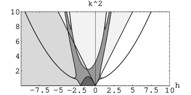
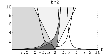
Figure 4: Asymptotical and mean–square stability regions for RI6 with $c_{1}=c_{2}=0$ on the left and for DDIRDI4 with $c_{1}=0$ and $c_{2}=\frac{1}{2}$ on the right.

If we choose $c_{1}=c_{2}=0$ and $c_{3}=c_{4}=1$ in (6), then we yield the explicit SRK scheme RI6 calculated in [20] which coincides for $m=1$ with the SRK scheme due to Platen [11, 18, 26]. If we apply Proposition 4.3 for RI6, then we obtain $\mathcal{R}_{AS}=\{(\hat{h},k)\in\mathbb{C}^{2}:|(1+\hat{h}+\frac{1}{2}\hat{h}^{2}+k^{2})^{2}-3(1+\hat{h})^{2}k^{2}||1+\hat{h}+\frac{1}{2}\hat{h}^{2}-\frac{1}{2}k^{2}|^{4}<1\}$ and $\mathcal{R}_{MS}=\{(\hat{h},k)\in\mathbb{C}^{2}:|1+\hat{h}+\frac{1}{2}\hat{h}^{2}|^{2}+|1+\hat{h}|^{2}|k|^{2}+\frac{1}{2}|k|^{4}<1\}$. The corresponding regions of stability are given in Figure 4. Further, we can choose $c_{1}=0$, $c_{2}=\frac{1}{2}$ and e.g. $c_{3}=c_{4}=1$ which defines the scheme DDIRDI4. Then, the DDIRDI4 scheme (3) is an advancement of the stochastic theta method DDIRDI2 with $\theta=\frac{1}{2}$. However, for DDIRDI4 we get $\mathcal{R}_{AS}=\{(\hat{h},k)\in\mathbb{C}^{2}:|(1+\frac{\hat{h}}{1-\frac{1}{2}\hat{h}}+k^{2})^{2}-3(1+\frac{\hat{h}-\frac{1}{4}\hat{h}^{2}}{1-\frac{1}{2}\hat{h}})^{2}k^{2}||1+\frac{\hat{h}}{1-\frac{1}{2}\hat{h}}-\frac{1}{2}k^{2}|^{4}<1\}$ and $\mathcal{R}_{MS}=\{(\hat{h},k)\in\mathbb{C}^{2}:|1+\frac{\hat{h}}{1-\frac{1}{2}\hat{h}}|^{2}+|1+\frac{\hat{h}-\frac{1}{4}\hat{h}^{2}}{1-\frac{1}{2}\hat{h}}|^{2}|k|^{2}+\frac{1}{2}|k|^{4}<1\}$. The regions of stability are given in Figure 4. Here, we can see that the good stability properties of the order one scheme DDIRDI2 are not carried over to the second order scheme DDIRDI4. Therefore, we are looking for further second order DDISRK methods with some better stability qualities.

It is usual to consider singly diagonally implicit Runge–Kutta methods for ODEs where all coefficients $A^{(0)}_{ii}$ are equal. Therefore, we assume that $c_{1}=c_{2}$ for the schemes (6) in the following. Then, the domains of stability are $\mathcal{R}_{AS}=\{(\hat{h},k)\in\mathbb{C}^{2}:|(1+\frac{\hat{h}+(\frac{1}{2}-2c_{1})\hat{h}^{2}}{(1-c_{1}\hat{h})^{2}}+k^{2})^{2}-3(1+\frac{\hat{h}-c_{1}\hat{h}^{2}}{(1-c_{1}\hat{h})^{2}})^{2}k^{2}||1+\frac{\hat{h}+(\frac{1}{2}-2c_{1})\hat{h}^{2}}{(1-c_{1}\hat{h})^{2}}-\frac{1}{2}k^{2}|^{4}<1\}$ and $\mathcal{R}_{MS}=\{(\hat{h},k)\in\mathbb{C}^{2}:|1+\frac{\hat{h}+(\frac{1}{2}-2c_{1})\hat{h}^{2}}{(1-c_{1}\hat{h})^{2}}|^{2}+|1+\frac{\hat{h}-c_{1}\hat{h}^{2}}{(1-c_{1}\hat{h})^{2}}|^{2}|k|^{2}+\frac{1}{2}|k|^{4}<1\}$ which depend on the coefficient $c_{1}$ of the scheme. In the following, we consider various values for the parameter $c_{1}$ of the DDISRK scheme (6) and we analyze the stability domain for $\lambda,\mu\in\mathbb{R}$. Therefore, we choose $c_{1}\in\{\frac{1}{4},\frac{1}{2},\frac{1}{2}+\frac{1}{6}\sqrt{3},1,\frac{3}{2},3\}$. Especially, we consider the case of $c_{1}=c_{2}=\frac{1}{2}+\frac{1}{6}\sqrt{3}$ and $c_{3}=c_{4}=1$ which we denote as the scheme DDIRDI5. Then, $A^{(0)}$ and $\alpha$ coincide with the coefficients of the well known deterministic SDIRK scheme which is $A$-stable and attains order $p_{D}=3$ for deterministic ODEs [5]. The corresponding stability regions are presented in Figures 5–7.

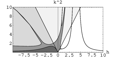
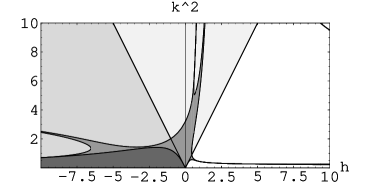
Figure 5: Stability regions for DDIRDI5 with $c_{1}=\frac{1}{4}$ on the left and $c_{1}=\frac{1}{2}$ on the right.

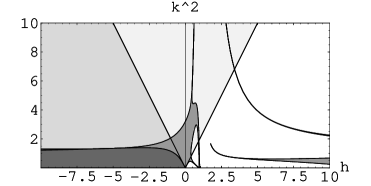
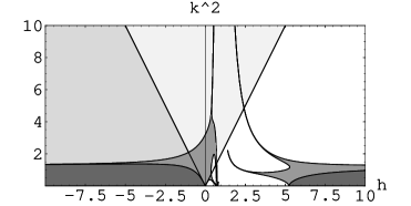
Figure 6: Stability regions for DDIRDI5 with $c_{1}=\frac{1}{2}+\frac{\sqrt{3}}{6}$ on the left and $c_{1}=1$ on the right.

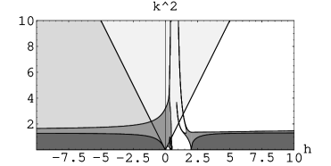
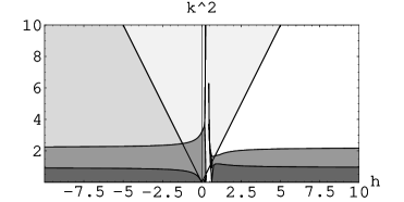
Figure 7: Stability regions for DDIRDI5 with $c_{1}=\frac{3}{2}$ on the left and $c_{1}=3$ on the right.

5 Numerical Experiments

We compare the efficiency of the proposed second order DDISRK schemes DDIRDI4 and DDIRDI5 with the second order drift–implicit SRK scheme DIPL1WM due to Platen ([11], p. 501). Therefore, we take the number of evaluations of the drift function $a$, of the diffusion functions $b^{j}$, $j=1,\ldots,m$, and the number of random numbers needed each step as a measure of the computational complexity for each considered scheme.

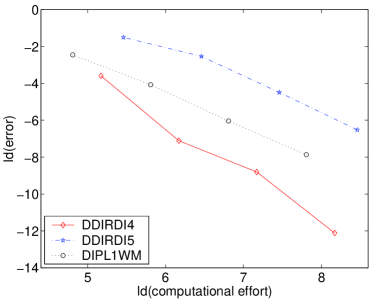
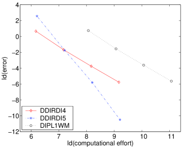
Figure 8: Error vs computational effort with double logarithmic scales for SDE (17) on the left and SDE (18) on the right hand side.

As a first example, we consider for $d=m=1$ the Itô SDE

$${\mathrm{d}}X_{t}=\big{(}\tfrac{1}{2}X_{t}+\sqrt{X_{t}^{2}+1}\big{)}\,{\mathrm{d}}t+\sqrt{X_{t}^{2}+1}\,{\mathrm{d}}W_{t}\,,\qquad X_{0}=0,$$ (17)

on the time interval $I=[0,2]$ with solution $X_{t}=\sinh(t+W_{t})$. Here, we choose $f(x)=p(\operatorname{arsinh}(x))$, where $p(z)=z^{3}-6z^{2}+8z$ is a polynomial. Then we calculate that $\operatorname{E}(f(X_{t}))=t^{3}-3t^{2}+2t$ which is approximated at time $t=2$ with step sizes $2^{-1},\ldots,2^{-4}$ and $10^{8}$ simulated trajectories. The results are presented on the left hand side of Fig. 8. As a second example, we consider a nonlinear SDE with a $10$–dimensional driving Wiener process

$$\begin{split}&{\mathrm{d}}X_{t}=X_{t}\,{\mathrm{d}}t+\frac{1}{10}\sqrt{X_{t}+\frac{1}{2}}\,{\mathrm{d}}W_{t}^{1}+\frac{1}{15}\sqrt{X_{t}+\frac{1}{4}}\,{\mathrm{d}}W_{t}^{2}+\frac{1}{20}\sqrt{X_{t}+\frac{1}{5}}\,{\mathrm{d}}W_{t}^{3}\\ &+\frac{1}{25}\sqrt{X_{t}+\frac{1}{10}}\,{\mathrm{d}}W_{t}^{4}+\frac{1}{40}\sqrt{X_{t}+\frac{1}{20}}\,{\mathrm{d}}W_{t}^{5}+\frac{1}{25}\sqrt{X_{t}+\frac{1}{2}}\,{\mathrm{d}}W_{t}^{6}+\frac{1}{20}\sqrt{X_{t}+\frac{1}{4}}\,{\mathrm{d}}W_{t}^{7}\\ &+\frac{1}{15}\sqrt{X_{t}+\frac{1}{5}}\,{\mathrm{d}}W_{t}^{8}+\frac{1}{20}\sqrt{X_{t}+\frac{1}{10}}\,{\mathrm{d}}W_{t}^{9}+\frac{1}{25}\sqrt{X_{t}+\frac{1}{20}}\,{\mathrm{d}}W_{t}^{10},\qquad X_{0}=1.\end{split}$$ (18)

with non-commutative noise. Here, we approximate the second moment of the solution $\operatorname{E}(X_{t}^{2})=-\frac{68013}{14629060}+(\frac{68013}{14629060}+1)\exp(\frac{731453}{360000}t)$ at time $t=1$ by $10^{8}$ simulated trajectories with step sizes $2^{0},\dots,2^{-3}$. The results are presented on the right hand side of Fig. 8. Here, the schemes DDIDRI4 and DDIDRI5 perform impressively better than the drift–implicit scheme DIPL1WM [11]. This is a result of the reduced complexity for the new class of efficient SRK schemes due to Rößler [20] which becomes significant especially for SDEs with high-dimensional driving Wiener processes.

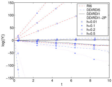
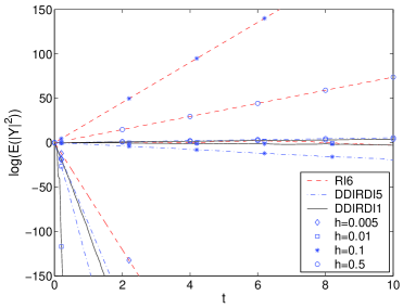
Figure 9: Asymptotical and MS–stability analysis for RI6, DDIRDI1 and DDIRDI5.

Next, we verify the theoretical results for the domains of stability of the proposed SRK methods by numerical experiments. Therefore, we consider the test equation (7) with parameters $\lambda=-200$, $\mu=\sqrt{5}$ and with initial value $X_{0}=1$ on the time interval $[0,10]$. We apply the second order explicit SRK scheme RI6 [20], the order one DDISRK scheme DDIRDI1 with two point as well as with three point distributed random variables and the order two DDISRK scheme DDIRDI5. We denote by DDIRDI1-2P the scheme DDIRDI1 if 2 point distributed random variables $\tilde{I}_{(j),n}$ are used instead of $\hat{I}_{(j),n}$.

In order to analyse the numerical asymptotically stability, a single approximation trajectory is simulated with each scheme under consideration for the step sizes $h=0.01$, $h=0.1$, $h=0.2$ and $h=0.5$. Then, we obtain the following theoretical results due to Proposition 4.2 and Proposition 4.3: the scheme RI6 is asymptotical stable for the step size $h=0.01$ and it is unstable for $h=0.1$, $h=0.2$ and $h=0.5$. DDIRDI1 and DDIRDI1-2P are stable for $h=0.01$ and $h=0.1$. In the case of $h=0.2$ only DDIRDI1-2P is stable while DDIRDI1 is unstable. Further, DDIRDI1 and DDIRDI1-2P are unstable for $h=0.5$. Finally, the scheme DDIRDI5 is asymptotical stable for $h=0.01$, $h=0.1$ and even for $h=0.2$, however it is unstable for $h=0.5$. The numerical results for a single trajectory $|Y_{n}|$ are plotted with logarithmic scale to the base 10 versus the time on the left hand side of Fig. 9. We remark that the results for DDIRDI1 with step size $h=0.01$ tend to zero after two steps and are thus not visible in Fig. 9.

For the analysis of the numerical MS–stability, the value $\operatorname{E}(|X_{t}|^{2})$ is approximated by Monte Carlo simulation with $10^{4}$ independent trajectories for the step sizes $h=0.005$, $h=0.01$, $h=0.1$ and $h=0.5$. Proposition 4.2 and Proposition 4.3 give the following results: RI6 is MS–stable for $h=0.005$ and MS–unstable for all other considered step sizes. DDIRDI1 and DDIRDI1-2P are MS–stable for $h=0.005$ and $h=0.01$, however MS–unstable for $h=0.1$ and $h=0.5$. Further, DDIRDI5 is MS–stable for step sizes $h=0.005$, $h=0.01$ and even for $h=0.1$ and MS–unstable for $h=0.5$. The corresponding numerical results of $\operatorname{E}(|Y_{n}|^{2})$ are presented with logarithmic scale to the base 10 versus the time on the right hand side of Fig. 9. Again, the numerical results exactly confirm our theoretical findings for the domains of stability.

References

- [1] K. Burrage, P. M. Burrage and T. Mitsui, Numerical solutions of stochastic differential equations – implementation and stability issues, J. Comput. Appl. Math., 125, (2000), 171–182.
- [2] K. Burrage and T. Tian, Implicit stochastic Runge–Kutta methods for stochastic differential equations, BIT, Vol. 44, (2004), 21–39.
- [3] K. Debrabant and A. Kværnø, Convergence of stochastic Runge–Kutta methods that use an iterative scheme to compute their internal stage values, SIAM J. Numer. Anal., Vol. 47, No. 1, (2008/09), 181–203.
- [4] K. Debrabant and A. Rößler, Families of efficient second order Runge–Kutta methods for the weak approximation of Itô stochastic differential equations, Applied Numerical Mathematics, Vol. 59, No. 3–4, (2009), 582–594.
- [5] E. Hairer and G. Wanner, Solving Ordinary Differential Equations II, Springer-Verlag, Berlin, 1996.
- [6] R. Z. Has’minskii, Stochastic stability of differential equations, Sijthoff & Noordhoff, Alphen aan den Rijn, Germantown, 1980.
- [7] D. B. Hernandez and R. Spigler, -stability of Runge–Kutta methods for systems with additive noise, BIT, Vol. 32, No.4, (1992), 620–633.
- [8] D. B. Hernandez and R. Spigler, Convergence and stability of implicit Runge–Kutta methods for systems with multiplicative noise, BIT, Vol. 33, No. 4, (1993), 654–669.
- [9] D. J. Higham, Mean–square and asymptotic stability of the stochastic theta method, SIAM J. Numer. Anal., Vol. 38, No. 3, (2000), 753–769.
- [10] N. Hofmann and E. Platen, Stability of Weak Numerical Schemes for Stochastic Differential Equations, Comput. Math. Appl., Vol. 28, No. 10–12, (1994), 45–57.
- [11] P. E. Kloeden and E. Platen, Numerical Solution of Stochastic Differential Equations (Applications of Mathematics 23, Springer-Verlag, Berlin, 1999).
- [12] Y. Komori, Weak first- or second-order implicit Runge–Kutta methods for stochastic differential equations with a scalar Wiener process, J. Comput. Appl. Math. (2007), doi:10.1016/j.cam.2007.06.024.
- [13] Y. Komori and T. Mitsui, Stable ROW-type weak scheme for stochastic differential equations, Monte Carlo Meth. Appl., Vol. 1, No. 4, (1995), 279–300.
- [14] G. N. Milstein and M. V. Tretyakov, Stochastic Numerics for Mathematical Physics, Scientific Computation, Springer-Verlag, Berlin, 2004.
- [15] G. N. Milstein, E. Platen and H. Schurz, Balanced implicit methods for stiff stochastic systems, SIAM J. Numer. Anal., Vol. 35, No. 3, (1998), 1010–1019.
- [16] W. P. Peterson, A general implicit splitting for stabilizing numerical simulations of Itô stochastic differential equations, SIAM J. Numer. Anal., Vol. 35, (1998), 1439–1451.
- [17] A. Rößler, Rooted tree analysis for order conditions of stochastic Runge–Kutta methods for the weak approximation of stochastic differential equations, Stochastic Anal. Appl. Vol. 24, No. 1, (2006), 97–134.
- [18] A. Rößler, Runge–Kutta methods for Itô stochastic differential equations with scalar noise, BIT, Vol. 46, No. 1, (2006), 97–110.
- [19] A. Rößler, Runge-Kutta methods for Stratonovich stochastic differential equation systems with commutative noise, J. Comput. Appl. Math., Vol. 164-165, (2004), 613–627.
- [20] A. Rößler, Second order Runge–Kutta methods for Itô stochastic differential equations, SIAM J. Numer. Anal., Vol. 47, No. 3, (2009), 1713–1738.
- [21] A. Rößler, Second order Runge–Kutta methods for Stratonovich stochastic differential equations, BIT, Vol. 47, No. 3, (2007), 657–680.
- [22] Y. Saito and T. Mitsui, T–stability of numerical scheme for stochastic differential equations, World Sci. Ser. Appl. Anal., Vol. 2, (1993), 333–344.
- [23] Y. Saito and T. Mitsui, Stability analysis of numerical schemes for stochastic differential equations, SIAM J. Numer. Anal., Vol. 33, No. 6, (1996), 2254–2267.
- [24] H. Schurz, Asymptotical mean square stability of an equilibrium point of some linear numerical solutions with multiplicative noise, Stochastic Anal. Appl., Vol. 14, (1996), 313–354.
- [25] H. Schurz, The invariance of asymptotic laws of linear stochastic systems under discretization, Z. Angew. Math. Mech., Vol. 79, No. 6, (1999), 375–382.
- [26] A. Tocino, Mean–square stability of second–order Runge–Kutta methods for stochastic differential equations, J. Comput. Appl. Math., Vol. 175, (2005), 355–367.
- [27] A. Tocino and J. Vigo-Aguiar, Weak second order conditions for stochastic Runge–Kutta methods, SIAM J. Sci. Comput., Vol. 24, No. 2, (2002), 507–523.