Families of efficient second order Runge-Kutta methods for the weak approximation of Itô stochastic differential equations

Abstract

Recently, a new class of second order Runge-Kutta methods for Itô stochastic differential equations with a multidimensional Wiener process was introduced by Rößler [10]. In contrast to second order methods earlier proposed by other authors, this class has the advantage that the number of function evaluations depends only linearly on the number of Wiener processes and not quadratically. In this paper, we give a full classification of the coefficients of all explicit methods with minimal stage number. Based on this classification, we calculate the coefficients of an extension with minimized error constant of the well-known RK32 method [2] to the stochastic case. For three examples, this method is compared numerically with known order two methods and yields very promising results.

and

Dedicated to Professor Karl Strehmel

1 Introduction

In recent years, the development of numerical methods for the approximation of stochastic differential equations (SDEs) has become a field of increasing interest, see. e.g [4, 7] and references therein. Whereas strong approximation methods are designed to obtain good pathwise solutions [1], weak approximation focuses on the expectation of functionals of the solution. Second order stochastic Runge-Kutta (SRK) methods for the weak approximation of SDEs were proposed by Kloeden and Platen [4], Komori [5], Mackevicius and Navikas [6], Tocino and Vigo-Aguiar [13], and the authors [3, 9]. However, these methods were not suitable for problems with high numbers $m$ of Wiener processes, because for these methods the number of function evaluations per step increases quadratically in $m$. Recently, new classes of SRK methods were introduced by Rößler [10, Roe06d] which overcome this problem. In Section 2 we present the one of these classes which is suitable for Itô SDEs. The aim of this paper is to give a full classification of all the explicit methods within this class with minimal stage number, which is done in Section 3. As an application, in Section 4 we extend the well known RK32 scheme [2] to an SRK method with minimized leading local error term. The performance of this method is illustrated by some numerical examples in section 5.

We denote by $(X(t))_{t\in I}$ the solution of the $d$-dimensional Itô SDE defined by

$${\mathrm{d}}X(t)=a(t,X(t))\,{\mathrm{d}}t+b(t,X(t))\,{\mathrm{d}}W(t),\qquad X({t_{0}})=x_{0},$$ (1)

with an $m$-dimensional Wiener process $(W(t))_{t\geq 0}$ and $I=[t_{0},T]$. We assume that the Borel-measurable coefficients $a:I\times\mathbb{R}^{d}\rightarrow\mathbb{R}^{d}$ and $b:I\times\mathbb{R}^{d}\rightarrow\mathbb{R}^{d\times m}$ satisfy a Lipschitz and a linear growth condition such that the Existence and Uniqueness Theorem [4] applies. In the following, let $b^{j}(t,x)=(b^{i,j}(t,x))_{1\leq i\leq d}\in\mathbb{R}^{d}$ denote the $j$th column of the diffusion matrix $b(t,x)$ for $j=1,\ldots,m$.

Let a discretization $I_{h}=\{t_{0},t_{1},\ldots,t_{N}\}$ with $t_{0}<t_{1}<\ldots<t_{N}=T$ of the time interval $I=[t_{0},T]$ with step sizes $h_{n}=t_{n+1}-t_{n}$ for $n=0,1,\ldots,N-1$ be given. Further, define $h=\max_{0\leq n<N}h_{n}$ as the maximum step size. Let $C_{P}^{l}(\mathbb{R}^{d},\mathbb{R})$ denote the space of all $g\in C^{l}(\mathbb{R}^{d},\mathbb{R})$ fulfilling a polynomial growth condition and let $g\in C_{P}^{k,l}(I\times\mathbb{R}^{d},\mathbb{R})$ if $g(\cdot,x)\in C^{k}(I,\mathbb{R})$ and $g(t,\cdot)\in C_{P}^{l}(\mathbb{R}^{d},\mathbb{R})$ for all $t\in I$ and $x\in\mathbb{R}^{d}$ [4].

Definition 1.1

A time discrete approximation $Y=(Y(t))_{t\in I_{h}}$ converges weakly with order $p$ to $X$ as $h\rightarrow 0$ at time $t\in I_{h}$ if for each $f\in C_{P}^{2(p+1)}(\mathbb{R}^{d},\mathbb{R})$ exist a constant $C_{f}$ and a finite $\delta_{0}>0$ such that

$$|\operatorname{E}(f(X(t)))-\operatorname{E}(f(Y(t)))|\leq C_{f}\,h^{p}$$ (2)

holds for each $h\in\,]0,\delta_{0}[\,$.

2 Stochastic Runge-Kutta methods

We consider the stochastic Runge-Kutta methods introduced in [10] for the weak approximation of SDE (1). Therefore, the $d$-dimensional approximation process $Y$ with $Y_{n}=Y(t_{n})$ of an explicit $s$-stage SRK method is defined by $Y_{0}=x_{0}$ and

$$\begin{split}Y_{n+1}=Y_{n}&+\sum_{i=1}^{s}\alpha_{i}\,a(t_{n}+c_{i}^{(0)}h_{n},H_{i}^{(0)})\,h_{n}\\ &+\sum_{i=1}^{s}\sum_{k=1}^{m}{\beta_{i}^{(1)}}\,b^{k}(t_{n}+c_{i}^{(1)}h_{n},H_{i}^{(k)})\,\hat{I}_{(k)}\\ &+\sum_{i=1}^{s}\sum_{k=1}^{m}{\beta_{i}^{(2)}}\,b^{k}(t_{n}+c_{i}^{(1)}h_{n},H_{i}^{(k)})\,\frac{\hat{I}_{(k,k)}}{\sqrt{h_{n}}}\\ &+\sum_{i=1}^{s}\sum_{k=1}^{m}{\beta_{i}^{(3)}}\,b^{k}(t_{n}+{c}_{i}^{(2)}h_{n},\hat{H}_{i}^{(k)})\,\hat{I}_{(k)}\\ &+\sum_{i=1}^{s}\sum_{k=1}^{m}{\beta_{i}^{(4)}}\,b^{k}(t_{n}+{c}_{i}^{(2)}h_{n},\hat{H}_{i}^{(k)})\,\sqrt{h_{n}}\end{split}$$ (3)

for $n=0,1,\ldots,N-1$ with stage values

$$H_{i}^{(0)} =Y_{n} +\sum_{j=1}^{i-1}A_{ij}^{(0)}\,a(t_{n}+c_{j}^{(0)}h_{n},H_{j}^{(0)})\,h_{n}$$

$$+\sum_{j=1}^{i-1}\sum_{l=1}^{m}{B_{ij}^{(0)}}\,b^{l}(t_{n}+c_{j}^{(1)}h_{n},H_{j}^{(l)})\,\hat{I}_{(l)}$$

$$H_{i}^{(k)} =Y_{n} +\sum_{j=1}^{i-1}A_{ij}^{(1)}\,a(t_{n}+c_{j}^{(0)}h_{n},H_{j}^{(0)})\,h_{n}$$

$$+\sum_{j=1}^{i-1}{B_{ij}^{(1)}}\,b^{k}(t_{n}+c_{j}^{(1)}h_{n},H_{j}^{(k)})\,\sqrt{h_{n}}$$

$$\hat{H}_{i}^{(k)} =Y_{n} +\sum_{j=1}^{s}{A}_{ij}^{(2)}\,a(t_{n}+c_{j}^{(0)}h_{n},H_{j}^{(0)})\,h_{n}$$

$$+\sum_{j=1}^{s}\sum_{\begin{subarray}{c}l=1\\ l\neq k\end{subarray}}^{m}{{B}_{ij}^{(2)}}\,b^{l}(t_{n}+c_{j}^{(1)}h_{n},H_{j}^{(l)})\,\frac{\hat{I}_{(k,l)}}{\sqrt{h_{n}}}$$

for $i=1,\ldots,s$ and $k=1,\ldots,m$. Here, $\alpha,\beta^{(1)},\dots,\beta^{(4)},c^{(q)}\in\mathbb{R}^{s}$ and $A^{(q)}$, $B^{(q)}\in\mathbb{R}^{s\times s}$ for $0\leq q\leq 2$ with $A_{ij}^{(q)}=B_{ij}^{(q)}=0$ for $j\geq i$ and $0\leq q\leq 1$ are the vectors and matrices of coefficients of the SRK method, $c^{(q)}=A^{(q)}e$ for $0\leq q\leq 2$ with a vector $e=(1,\ldots,1)^{T}$. In the following, the product of column vectors is defined component-wise. The coefficients of the SRK method (3) are determined by the following Butcher tableau:

$c^{(0)}$	${A}^{(0)}$	$B^{(0)}$
$c^{(1)}$	${A}^{(1)}$	$B^{(1)}$
$c^{(2)}$	${A}^{(2)}$	$B^{(2)}$
	$\alpha^{T}$	${\beta^{(1)}}^{T}$	${\beta^{(2)}}^{T}$
		${\beta^{(3)}}^{T}$	${\beta^{(4)}}^{T}$

$\hat{I}_{(k)}$ are three-point distributed random variables with $\operatorname{P}(\hat{I}_{(k)}=\pm\sqrt{3\,h_{n}})=\frac{1}{6}$ and $\operatorname{P}(\hat{I}_{(k)}=0)=\frac{2}{3}$. Further, $\hat{I}_{(k,l)}$ are defined by

$$\hat{I}_{(k,l)}=\begin{cases}\tfrac{1}{2}(\hat{I}_{(k)}\hat{I}_{(l)}-\sqrt{h_{n}}\tilde{I}_{(k)})&\text{if }k<l\\ \tfrac{1}{2}(\hat{I}_{(k)}\hat{I}_{(l)}+\sqrt{h_{n}}\tilde{I}_{(l)})&\text{if }l<k\\ \tfrac{1}{2}(\hat{I}_{(k)}^{2}-h_{n})&\text{if }k=l\end{cases}$$ (4)

with two point distributed random variables $\tilde{I}_{(k)}$ satisfying $\operatorname{P}(\tilde{I}_{(k)}=\pm\sqrt{h_{n}})=\tfrac{1}{2}$.

By the application of the multi–colored rooted tree analysis [8], order conditions for the coefficients of the SRK method (3) can be easily determined. As a result of this, the following Theorem 2.1 due to Rößler [10] gives order conditions for the SRK method (3) up to order two.

Theorem 2.1

Let $a^{i},b^{i,j}\in C_{P}^{2,4}(I\times\mathbb{R}^{d},\mathbb{R})$ for $1\leq i\leq d$, $1\leq j\leq m$. If the coefficients of the SRK method (3) fulfill the equations

$$1 .\quad\alpha^{T}e=1\qquad\qquad 2.\quad {\beta^{(4)}}^{T}e=0\qquad\qquad 3.\quad {\beta^{(3)}}^{T}e=0$$

$$4 .\quad({\beta^{(1)}}^{T}e)^{2}=1\qquad\qquad 5.\quad {\beta^{(2)}}^{T}e=0\qquad\qquad 6.\quad {\beta^{(1)}}^{T}{B^{(1)}}e=0$$

$$7 .\quad{\beta^{(4)}}^{T}A^{(2)}e=0\qquad 8.\quad {\beta^{(3)}}^{T}{B^{(2)}}e=0\qquad 9.\quad {\beta^{(4)}}^{T}({B^{(2)}}e)^{2}=0$$

then the method attains order 1 in the weak sense. In addition, if $a^{i},b^{i,j}\in C_{P}^{3,6}(I\times\mathbb{R}^{d},\mathbb{R})$ for $1\leq i\leq d$, $1\leq j\leq m$ and if the equations

$$10 .\quad\alpha^{T}A^{(0)}e=\tfrac{1}{2}\qquad\qquad\qquad\qquad\quad 11.\quad \alpha^{T}(B^{(0)}e)^{2}=\tfrac{1}{2}$$

$$12 .\quad({\beta^{(1)}}^{T}e)(\alpha^{T}B^{(0)}e)=\tfrac{1}{2}\qquad\qquad 13.\quad ({\beta^{(1)}}^{T}e)({\beta^{(1)}}^{T}A^{(1)}e)=\tfrac{1}{2}$$

$$14 .\quad{\beta^{(3)}}^{T}A^{(2)}e=0\qquad\qquad 15.\quad {\beta^{(2)}}^{T}B^{(1)}e=1$$

$$16 .\quad{\beta^{(4)}}^{T}B^{(2)}e=1\qquad\qquad 17.\quad ({\beta^{(1)}}^{T}e)({\beta^{(1)}}^{T}(B^{(1)}e)^{2})=\tfrac{1}{2}$$

$$18 .\quad({\beta^{(1)}}^{T}e)({\beta^{(3)}}^{T}(B^{(2)}e)^{2})=\tfrac{1}{2}\qquad 19.\quad {\beta^{(1)}}^{T}(B^{(1)}(B^{(1)}e))=0$$

$$20 .\quad{\beta^{(3)}}^{T}(B^{(2)}(B^{(1)}e))=0\qquad 21.\quad {\beta^{(3)}}^{T}(B^{(2)}(B^{(1)}(B^{(1)}e)))=0$$

$$22 .\quad{\beta^{(1)}}^{T}(A^{(1)}(B^{(0)}e))=0\qquad 23.\quad {\beta^{(3)}}^{T}(A^{(2)}(B^{(0)}e))=0$$

$$24 .\quad{\beta^{(4)}}^{T}(A^{(2)}e)^{2}=0\qquad 25.\quad {\beta^{(4)}}^{T}(A^{(2)}(A^{(0)}e))=0$$

$$26 .\quad\alpha^{T}(B^{(0)}(B^{(1)}e))=0\qquad 27.\quad {\beta^{(2)}}^{T}A^{(1)}e=0$$

$$28 .\quad{\beta^{(1)}}^{T}((A^{(1)}e)(B^{(1)}e))=0\qquad 29.\quad {\beta^{(3)}}^{T}((A^{(2)}e)(B^{(2)}e))=0$$

$$30 .\quad{\beta^{(4)}}^{T}(A^{(2)}(B^{(0)}e))=0\qquad 31.\quad {\beta^{(2)}}^{T}(A^{(1)}(B^{(0)}e))=0$$

$$32 .\quad{\beta^{(4)}}^{T}((B^{(2)}e)^{2}(A^{(2)}e))=0\qquad 33.\quad {\beta^{(4)}}^{T}(A^{(2)}(B^{(0)}e)^{2})=0$$

$$34 .\quad{\beta^{(2)}}^{T}(A^{(1)}(B^{(0)}e)^{2})=0\qquad 35.\quad {\beta^{(1)}}^{T}(B^{(1)}(A^{(1)}e))=0$$

$$36 .\quad{\beta^{(3)}}^{T}(B^{(2)}(A^{(1)}e))=0\qquad 37.\quad {\beta^{(2)}}^{T}(B^{(1)}e)^{2}=0$$

$$38 .\quad{\beta^{(4)}}^{T}(B^{(2)}(B^{(1)}e))=0\qquad 39.\quad {\beta^{(2)}}^{T}(B^{(1)}(B^{(1)}e))=0$$

$$40 .\quad{\beta^{(1)}}^{T}(B^{(1)}e)^{3}=0\qquad 41.\quad {\beta^{(3)}}^{T}(B^{(2)}e)^{3}=0$$

$$42 .\quad{\beta^{(1)}}^{T}(B^{(1)}(B^{(1)}e)^{2})=0\qquad 43.\quad {\beta^{(3)}}^{T}(B^{(2)}(B^{(1)}e)^{2})=0$$

$$44 .\quad{\beta^{(4)}}^{T}(B^{(2)}e)^{4}=0\qquad 45.\quad {\beta^{(4)}}^{T}(B^{(2)}(B^{(1)}e))^{2}=0$$

$$46 .\quad{\beta^{(4)}}^{T}((B^{(2)}e)(B^{(2)}(B^{(1)}e)))=0 47.\quad \alpha^{T}((B^{(0)}e)(B^{(0)}(B^{(1)}e)))=0$$

$$48 .\quad{\beta^{(1)}}^{T}((A^{(1)}(B^{(0)}e))(B^{(1)}e))=0 49.\quad {\beta^{(3)}}^{T}((A^{(2)}(B^{(0)}e))(B^{(2)}e))=0$$

$$50 .\quad{\beta^{(1)}}^{T}(A^{(1)}(B^{(0)}(B^{(1)}e)))=0 51.\quad {\beta^{(3)}}^{T}(A^{(2)}(B^{(0)}(B^{(1)}e)))=0$$

$$52 .\quad{\beta^{(4)}}^{T}((B^{(2)}(A^{(1)}e))(B^{(2)}e))=0 53.\quad {\beta^{(1)}}^{T}(B^{(1)}(A^{(1)}(B^{(0)}e)))=0$$

$$54 .\quad{\beta^{(3)}}^{T}(B^{(2)}(A^{(1)}(B^{(0)}e)))=0 55.\quad {\beta^{(1)}}^{T}((B^{(1)}e)(B^{(1)}(B^{(1)}e)))=0$$

$$56 .\quad{\beta^{(3)}}^{T}((B^{(2)}e)(B^{(2)}(B^{(1)}e)))=0 57.\quad {\beta^{(1)}}^{T}(B^{(1)}(B^{(1)}(B^{(1)}e)))=0$$

$$58 .\quad{\beta^{(4)}}^{T}((B^{(2)}e)(B^{(2)}(B^{(1)}e)^{2}))=0 59.\quad {\beta^{(4)}}^{T}((B^{(2)}e)(B^{(2)}(B^{(1)}(B^{(1)}e))))=0$$

are fulfilled, then the SRK method (3) attains order 2 in the weak sense.

It turns out that explicit order one SRK methods need at least $s=1$ stage while order two SRK methods need $s\geq 3$ stages. This is due to e.g. conditions 4., 6. and 17., which can not be fulfilled in the case of $s\leq 2$ stages for explicit order two SRK methods. In the following, we distinguish between the stochastic and the deterministic order of convergence. Let $p_{S}=p$ denote the order of convergence of the SRK method if it is applied to an SDE and let $p_{D}$ with $p_{D}\geq p_{S}$ denote the order of convergence of the SRK method if it is applied to a deterministic ordinary differential equation (ODE), i.e., SDE (1) with $b\equiv 0$. We also write $(p_{D},p_{S})$ in the following.

3 Parameter families for SRK methods

3.1 Coefficients for SRK methods of order (1,1)

First, we analyze explicit SRK methods (3) of order $p_{D}=p_{S}=1$ with $s=1$ stage. Considering the order one conditions 1.–9. in Theorem 2.1, the corresponding coefficients are uniquely determined for $c_{1}\in\{-1,1\}$ by

$$\alpha_{1}=1,\qquad\beta_{1}^{(1)}=c_{1},\qquad\beta_{1}^{(2)}=0,\qquad\beta_{1}^{(3)}=0,\qquad\beta_{1}^{(4)}=0.$$ (5)

The resulting class of SRK schemes coincides with the well-known Euler-Maruyama scheme.

3.2 Coefficients for SRK methods of order (2,1)

Next, we consider the case of $s=2$ stage explicit SRK methods (3). As already mentioned in Section 2, it is not possible to attain order $p_{S}=2$. However, we can find some SRK methods of order $p_{D}=2$ and $p_{S}=1$ corresponding to the following parameter family: From condition 1. of Theorem 2.1 follows $\alpha_{1}=1-\alpha_{2}$ and taking into account the order two condition 10. we obtain $\alpha_{2}=\frac{1}{2A^{(0)}_{21}}$ for $A^{(0)}_{21}\neq 0$. Further, condition 2. yields $\beta^{(4)}_{1}=-\beta^{(4)}_{2}$, condition 3. results in $\beta^{(3)}_{1}=-\beta^{(3)}_{2}$ and condition 5. is fulfilled if $\beta^{(2)}_{1}=-\beta^{(2)}_{2}$ while condition 4. holds for $\beta^{(1)}_{1}=c_{1}-\beta^{(1)}_{2}$ with $c_{1}\in\{-1,1\}$. Finally, considering condition 6. we need that $\beta^{(1)}_{2}=0$ or $B^{(1)}_{21}=0$, considering condition 8. analogously that $\beta^{(3)}_{2}=0$ or $B^{(2)}_{11}+B^{(2)}_{12}=B^{(2)}_{21}+B^{(2)}_{22}$ and for condition 7. and 9. that $\beta^{(4)}_{2}=0$ or $A^{(2)}_{11}+A^{(2)}_{12}=A^{(2)}_{21}+A^{(2)}_{22}$ and $(B^{(2)}_{11}+B^{(2)}_{12})^{2}=(B^{(2)}_{21}+B^{(2)}_{22})^{2}$ hold. Thus, this class of SRK methods is determined by

$$\alpha^{T} =\begin{bmatrix}1-\frac{1}{2c_{2}}&&\frac{1}{2c_{2}}\end{bmatrix}, \quad\quad{\beta^{(1)}}^{T} =\begin{bmatrix}c_{1}-c_{4}&&c_{4}\end{bmatrix}, \quad\quad{\beta^{(2)}}^{T} =\begin{bmatrix}c_{5}&&-c_{5}\end{bmatrix},$$

$${\beta^{(3)}}^{T} =\begin{bmatrix}c_{6}&&-c_{6}\end{bmatrix}, \quad{\beta^{(4)}}^{T} =\begin{bmatrix}c_{7}&&-c_{7}\end{bmatrix},$$

$$A^{(0)} =\begin{bmatrix}0&&0\\ c_{2}&&0\end{bmatrix}, \quad A^{(1)} =\begin{bmatrix}0&&0\\ c_{8}&&0\end{bmatrix}, \quad A^{(2)} =\begin{bmatrix}c_{9}&&c_{10}\\ c_{11}&&c_{12}\end{bmatrix},$$

$$B^{(0)} =\begin{bmatrix}0&&0\\ c_{3}&&0\end{bmatrix}, \quad B^{(1)} =\begin{bmatrix}0&&0\\ c_{17}&&0\end{bmatrix}, \quad B^{(2)} =\begin{bmatrix}c_{13}&&c_{14}\\ c_{15}&&c_{16}\end{bmatrix},$$ (6)

for $c_{1}\in\{-1,1\}$ and $c_{2},\ldots,c_{17}\in\mathbb{R}$ with $c_{2}\neq 0$, $c_{4}\,c_{17}=0$, $c_{6}(c_{13}+c_{14}-c_{15}-c_{16})=0$, $c_{7}(c_{9}+c_{10}-c_{11}-c_{12})=0$ and $c_{7}((c_{13}+c_{14})^{2}-(c_{15}+c_{16})^{2})=0$.

3.3 Coefficients for SRK methods of order (2,2)

Now, we consider explicit SRK methods (3) of order $p_{D}=p_{S}=2$ with $s=3$ stages. Then, the SRK schemes of the class under consideration are completely characterized by the following families of coefficients which follow from the order conditions in Theorem 2.1:

We have $\alpha_{1}=1-\alpha_{2}-\alpha_{3}$ due to condition 1. From condition 4. it follows that $\beta^{(1)}_{3}=c_{1}-\beta^{(1)}_{2}-\beta^{(1)}_{1}$ with $c_{1}\in\{-1,1\}$. Due to conditions 2., 3., 7., 24., 16., 14., 18. and 8. we need $\sum_{i=1}^{3}A^{(2)}_{1i}=\sum_{i=1}^{3}A^{(2)}_{2i}=\sum_{i=1}^{3}A^{(2)}_{3i}$. From conditions 3., 8., 18. and 41. follows that $\sum_{i,j=1}^{3}B^{(2)}_{i,j}=0$ and that ${{b}}_{i}:=\sum_{j=1}^{3}B^{(2)}_{ij}$, $i=1,2,3$ are pairwise different. Further, we have $\beta^{(3)}_{1}=\frac{c_{1}}{2({{b}}_{1}-{{b}}_{2})({{b}}_{2}+2{{b}}_{1})}$, $\beta^{(3)}_{2}=\frac{c_{1}}{2({{b}}_{2}-{{b}}_{1})({{b}}_{1}+2{{b}}_{2})}$, $\beta^{(3)}_{3}=\frac{c_{1}}{2(2{{b}}_{1}+{{b}}_{2})({{b}}_{1}+2{{b}}_{2})}$. From conditions 2., 9. and 16. we obtain $\beta^{(4)}_{1}=\frac{{{b}}_{1}}{({{b}}_{1}-{{b}}_{2})({{b}}_{2}+2{{b}}_{1})}$, $\beta^{(4)}_{2}=\frac{{{b}}_{2}}{({{b}}_{2}-{{b}}_{1})({{b}}_{1}+2{{b}}_{2})}$, $\beta^{(4)}_{3}=\frac{-{{b}}_{1}-{{b}}_{2}}{(2{{b}}_{1}+{{b}}_{2})({{b}}_{1}+2{{b}}_{2})}$. With 44. it follows now from the above that exactly for one $i$ from $1,2,3$ it holds ${{b}}_{i}=0$. Without loss of generality we can assume that ${{b}}_{1}=0$. Due to conditions 15. and 37. we need $B^{(1)}_{21}\neq 0$ and from conditions 17. and 40. follows $\beta^{(1)}_{3}\neq 0$. Now, by condition 19. follows that $B^{(1)}_{32}=0$ and we deduce from 6., 17. and 40. that $B^{(1)}_{31}=-B^{(1)}_{21}$. With conditions 5., 15. and 37. follows that $\beta^{(2)}_{2}=\frac{1}{2B^{(1)}_{21}}$, $\beta^{(2)}_{3}=-\frac{1}{2B^{(1)}_{21}}$ and $\beta^{(2)}_{1}=0$. Conditions 4., 6. and 17. yield $\beta^{(1)}_{1}=c_{1}-\frac{c_{1}}{2(B^{(1)}_{21})^{2}}$ and $\beta^{(1)}_{2}=\beta^{(1)}_{3}=\frac{c_{1}}{4(B^{(1)}_{21})^{2}}$. From condition 56. and 58. we obtain $B^{(2)}_{22}=-B^{(2)}_{33}$ and $B^{(2)}_{23}=-B^{(2)}_{33}$. Condition 43. yields now $B^{(2)}_{12}=-B^{(2)}_{13}$. Condition 46. gives $B^{(2)}_{32}=B^{(2)}_{33}$. Condition 20. leads to $B^{(2)}_{13}=0$. Now, due to 13. and 28. we need that $A^{(1)}_{21}=(B^{(1)}_{21})^{2}$ and $A^{(1)}_{31}=(B^{(1)}_{21})^{2}-A^{(1)}_{32}$.
To fulfill 11., 12., 22., 23., 30. and 33., we obtain the following cases:

1. $B^{(0)}_{21}=0,B^{(0)}_{31}+B^{(0)}_{32}=c_{1},\alpha_{3}=\frac{1}{2},A^{(2)}_{13}=A^{(2)}_{23}=A^{(2)}_{33}$,

2. $A^{(1)}_{32}=0,B^{(0)}_{21}=c_{1},B^{(0)}_{31}+B^{(0)}_{32}=0,\alpha_{2}=\frac{1}{2},A^{(2)}_{12}=A^{(2)}_{22}=A^{(2)}_{32}$,

3. $A^{(1)}_{32}=0,B^{(0)}_{21}=B^{(0)}_{31}+B^{(0)}_{32}=c_{1},\alpha_{2}+\alpha_{3}=\frac{1}{2},A^{(2)}_{12}+A^{(2)}_{13}=A^{(2)}_{22}+A^{(2)}_{23}=A^{(2)}_{32}+A^{(2)}_{33}$,

4. $A^{(1)}_{32}=0,B^{(0)}_{21}\neq 0\neq B^{(0)}_{31}+B^{(0)}_{32}\neq B^{(0)}_{21},A^{(2)}_{22}=A^{(2)}_{32},A^{(2)}_{23}=A^{(2)}_{33},A^{(2)}_{12}=A^{(2)}_{32}+(A^{(2)}_{33}-A^{(2)}_{13})\frac{B^{(0)}_{31}+B^{(0)}_{32}}{B^{(0)}_{21}}$, $\alpha_{2}=\frac{1}{2}\frac{1-c_{1}(B^{(0)}_{31}+B^{(0)}_{32})}{B^{(0)}_{21}(B^{(0)}_{21}-B^{(0)}_{31}-B^{(0)}_{32})}$, $\alpha_{3}=-\frac{1}{2}\frac{1-c_{1}B^{(0)}_{21}}{(B^{(0)}_{31}+B^{(0)}_{32})(B^{(0)}_{21}-B^{(0)}_{31}-B^{(0)}_{32})}$.

However, from 26. and 51. it follows

1. $B^{(0)}_{32}=0$ or

2. $\alpha_{3}=0,A^{(2)}_{23}+A^{(2)}_{33}=2A^{(2)}_{13}$.

Finally, the equations 10. and 25. imply the cases

1. $\alpha_{2}(A^{(2)}_{23}-A^{(2)}_{33})\neq\alpha_{3}(A^{(2)}_{22}-A^{(2)}_{32})$, $A^{(0)}_{21}=\frac{1}{2}\frac{A^{(2)}_{23}-A^{(2)}_{33}}{\alpha_{2}(A^{(2)}_{23}-A^{(2)}_{33})-\alpha_{3}(A^{(2)}_{22}-A^{(2)}_{32})}$, $A^{(0)}_{31}=-\frac{1}{2}\frac{A^{(2)}_{22}-A^{(2)}_{32}}{\alpha_{2}(A^{(2)}_{23}-A^{(2)}_{33})-\alpha_{3}(A^{(2)}_{22}-A^{(2)}_{32})}-A^{(0)}_{32}$,

2. $A^{(2)}_{23}=A^{(2)}_{33}$, $A^{(2)}_{22}=A^{(2)}_{32}$, $\alpha_{2}\neq 0$, $A^{(0)}_{21}=\frac{1-2\alpha_{3}(A^{(0)}_{31}+A^{(0)}_{32})}{2\alpha_{2}}$,

3. $A^{(2)}_{23}=A^{(2)}_{33}$, $A^{(2)}_{22}=A^{(2)}_{32}$, $\alpha_{2}=0$, $\alpha_{3}\neq 0$, $A^{(0)}_{31}=\frac{1}{2\alpha_{3}}-A^{(0)}_{32}$.

With these settings, all the remaining order conditions are now fulfilled.
Summarizing our results, we have the following classification for the SRK schemes of order $p_{D}=p_{S}=2$ for the considered class with $s=3$ stages: For $c_{1}\in\{-1,1\}$ and $c_{2},c_{3},c_{4},c_{5}\in\mathbb{R}$ with $c_{3}\neq 0$ and $c_{4}\neq 0$ holds

$${\beta^{(1)}}^{T} =\begin{bmatrix}c_{1}-\frac{c_{1}}{2c_{3}^{2}}&&\frac{c_{1}}{4c_{3}^{2}}&&\frac{c_{1}}{4c_{3}^{2}}\end{bmatrix}, \quad\quad{\beta^{(2)}}^{T} =\begin{bmatrix}0&&\frac{1}{2c_{3}}&&-\frac{1}{2c_{3}}\end{bmatrix},$$ (7)

$${\beta^{(4)}}^{T} =\begin{bmatrix}0&&\frac{1}{2c_{4}}&&-\frac{1}{2c_{4}}\end{bmatrix}, \quad\quad{\beta^{(3)}}^{T} =\begin{bmatrix}-\frac{c_{1}}{2c_{4}^{2}}&&\frac{c_{1}}{4c_{4}^{2}}&&\frac{c_{1}}{4c_{4}^{2}}\end{bmatrix},$$ (8)

$$A^{(1)} =\begin{bmatrix}0&&0&&0\\ c_{3}^{2}&&0&&0\\ c_{3}^{2}-c_{2}&&c_{2}&&0\end{bmatrix}, \quad\quad B^{(1)} =\begin{bmatrix}0&&0&&0\\ c_{3}&&0&&0\\ -c_{3}&&0&&0\end{bmatrix},$$ (9)

$$B^{(2)} =\begin{bmatrix}0&&0&&0\\ c_{4}+2c_{5}&&-c_{5}&&-c_{5}\\ -c_{4}-2c_{5}&&c_{5}&&c_{5}\end{bmatrix}.$$ (10)

Now, the following cases are possible:

In the case 1ai) we get with $c_{6},\dots,c_{12}\in\mathbb{R}$ that

$$\alpha^{T}=\begin{bmatrix}\frac{1}{2}-c_{11}&&c_{11}&&\frac{1}{2}\end{bmatrix},\quad B^{(0)}=\begin{bmatrix}0&&0&&0\\ 0&&0&&0\\ c_{1}&&0&&0\end{bmatrix},$$ (11)

$$A^{(0)}=\begin{bmatrix}0&&0&&0\\ 0&&0&&0\\ c_{12}&&1-c_{12}&&0\end{bmatrix},\quad A^{(2)}=\begin{bmatrix}c_{6}-c_{7}&&c_{7}&&c_{8}\\ c_{6}-c_{9}&&c_{9}&&c_{8}\\ c_{6}-c_{10}&&c_{10}&&c_{8}\end{bmatrix}.$$ (12)

In the case 1aii) we obtain with $c_{6},\dots,c_{12}\in\mathbb{R}$ and $c_{10}\neq 0$ that

$$\alpha^{T}=\begin{bmatrix}\frac{1}{2}-c_{10}&&c_{10}&&\frac{1}{2}\end{bmatrix},\quad B^{(0)}=\begin{bmatrix}0&&0&&0\\ 0&&0&&0\\ c_{1}&&0&&0\end{bmatrix},$$ (13)

$$A^{(0)}=\begin{bmatrix}0&&0&&0\\ \frac{1-c_{11}}{2c_{10}}&&0&&0\\ c_{11}-c_{12}&&c_{12}&&0\end{bmatrix},\quad A^{(2)}=\begin{bmatrix}c_{6}-c_{7}&&c_{7}&&c_{8}\\ c_{6}-c_{9}&&c_{9}&&c_{8}\\ c_{6}-c_{9}&&c_{9}&&c_{8}\end{bmatrix}.$$ (14)

Considering the case 1aiii) we obtain with $c_{6},\dots,c_{11}\in\mathbb{R}$ that

$$\alpha^{T}=\begin{bmatrix}\frac{1}{2}&&0&&\frac{1}{2}\end{bmatrix},\quad B^{(0)}=\begin{bmatrix}0&&0&&0\\ 0&&0&&0\\ c_{1}&&0&&0\end{bmatrix},$$ (15)

$$A^{(0)}=\begin{bmatrix}0&&0&&0\\ c_{10}&&0&&0\\ 1-c_{11}&&c_{11}&&0\end{bmatrix},\quad A^{(2)}=\begin{bmatrix}c_{6}-c_{7}&&c_{7}&&c_{8}\\ c_{6}-c_{9}&&c_{9}&&c_{8}\\ c_{6}-c_{9}&&c_{9}&&c_{8}\end{bmatrix}.$$ (16)

For the case 2ai) we get with $c_{2}=0$ in (9) and $c_{6},\dots,c_{12}\in\mathbb{R}$, $c_{9}\neq c_{10}$ the coefficients

$$\alpha^{T}=\begin{bmatrix}\frac{1}{2}-c_{11}&&\frac{1}{2}&&c_{11}\end{bmatrix},\quad B^{(0)}=\begin{bmatrix}0&&0&&0\\ c_{1}&&0&&0\\ 0&&0&&0\end{bmatrix},$$ (17)

$$A^{(0)}=\begin{bmatrix}0&&0&&0\\ 1&&0&&0\\ c_{12}&&-c_{12}&&0\end{bmatrix},\quad A^{(2)}=\begin{bmatrix}c_{6}-c_{8}&&c_{7}&&c_{8}\\ c_{6}-c_{9}&&c_{7}&&c_{9}\\ c_{6}-c_{10}&&c_{7}&&c_{10}\end{bmatrix}.$$ (18)

In the case 2aii) we obtain with $c_{2}=0$ in (9) and $c_{6},\dots,c_{12}\in\mathbb{R}$ the coefficients

$$\alpha^{T}=\begin{bmatrix}\frac{1}{2}-c_{10}&&\frac{1}{2}&&c_{10}\end{bmatrix},\quad B^{(0)}=\begin{bmatrix}0&&0&&0\\ c_{1}&&0&&0\\ 0&&0&&0\end{bmatrix},$$ (19)

$$A^{(0)}=\begin{bmatrix}0&&0&&0\\ 1-2c_{10}c_{11}&&0&&0\\ c_{11}-c_{12}&&c_{12}&&0\end{bmatrix},\quad A^{(2)}=\begin{bmatrix}c_{6}-c_{8}&&c_{7}&&c_{8}\\ c_{6}-c_{9}&&c_{7}&&c_{9}\\ c_{6}-c_{9}&&c_{7}&&c_{9}\end{bmatrix}.$$ (20)

For the case 2bi) we get with $c_{2}=0$ in (9) and $c_{6},\dots,c_{11}\in\mathbb{R}$, $c_{8}\neq c_{9}$ the coefficients

$$\alpha^{T}=\begin{bmatrix}\frac{1}{2}&&\frac{1}{2}&&0\end{bmatrix},\quad B^{(0)}=\begin{bmatrix}0&&0&&0\\ c_{1}&&0&&0\\ c_{10}&&-c_{10}&&0\end{bmatrix},$$ (21)

$$A^{(0)}=\begin{bmatrix}0&&0&&0\\ 1&&0&&0\\ c_{11}&&-c_{11}&&0\end{bmatrix},\quad A^{(2)}=\begin{bmatrix}c_{6}-c_{8}&&c_{7}&&c_{8}\\ c_{6}-c_{9}&&c_{7}&&c_{9}\\ c_{6}-2c_{8}+c_{9}&&c_{7}&&2c_{8}-c_{9}\end{bmatrix}.$$ (22)

In the cases 2bii), 3bii) respectively 4bii) we obtain with $c_{2}=0$ in (9) and $c_{6},\dots,c_{12}\in\mathbb{R}$

$$\alpha^{T}=\begin{bmatrix}\frac{1}{2}&&\frac{1}{2}&&0\end{bmatrix},\,\,\,\,B^{(0)}=\begin{bmatrix}0&&0&&0\\ c_{1}&&0&&0\\ c_{9}-c_{10}&&c_{10}&&0\end{bmatrix},$$ (23)

$$A^{(0)}=\begin{bmatrix}0&&0&&0\\ 1&&0&&0\\ c_{11}&&c_{12}&&0\end{bmatrix},\quad A^{(2)}=\begin{bmatrix}c_{6}&&c_{7}&&c_{8}\\ c_{6}&&c_{7}&&c_{8}\\ c_{6}&&c_{7}&&c_{8}\end{bmatrix},$$ (24)

where $c_{9}=0$ in the case 2bii), $c_{9}=c_{1}$ for 3bii) and $0\neq c_{9}\neq c_{1}$ for 4bii), respectively.
Considering the case 3ai) we find with $c_{2}=0$ in (9) and $c_{6},\dots,c_{12}\in\mathbb{R}$, $c_{9}\neq c_{10}$ that

$$\alpha^{T}=\begin{bmatrix}\frac{1}{2}&&\frac{1}{2}-c_{11}&&c_{11}\end{bmatrix},B^{(0)}=\begin{bmatrix}0&&0&&0\\ c_{1}&&0&&0\\ c_{1}&&0&&0\end{bmatrix},$$ (25)

$$A^{(0)}=\begin{bmatrix}0&&0&&0\\ 1&&0&&0\\ 1-c_{12}&&c_{12}&&0\end{bmatrix},\,\,\quad A^{(2)}=\begin{bmatrix}c_{6}&&c_{7}&&c_{8}\\ c_{6}&&c_{9}&&c_{7}+c_{8}-c_{9}\\ c_{6}&&c_{10}&&c_{7}+c_{8}-c_{10}\end{bmatrix}.$$ (26)

For the case 3aii) we obtain with $c_{2}=0$ in (9) and $c_{6},\dots,c_{12}\in\mathbb{R}$, $c_{10}\neq\frac{1}{2}$, that

$$\alpha^{T}=\begin{bmatrix}\frac{1}{2}&&\frac{1}{2}-c_{10}&&c_{10}\end{bmatrix},B^{(0)}=\begin{bmatrix}0&&0&&0\\ c_{1}&&0&&0\\ c_{1}&&0&&0\end{bmatrix},$$ (27)

$$A^{(0)}=\begin{bmatrix}0&&0&&0\\ \frac{1-2c_{10}c_{11}}{1-2c_{10}}&&0&&0\\ c_{11}-c_{12}&&c_{12}&&0\end{bmatrix},\,\,\quad A^{(2)}=\begin{bmatrix}c_{6}&&c_{7}&&c_{8}\\ c_{6}&&c_{9}&&c_{7}+c_{8}-c_{9}\\ c_{6}&&c_{9}&&c_{7}+c_{8}-c_{9}\end{bmatrix}.$$ (28)

In the case 3aiii) respectively 4aiii) we get with $c_{2}=0$ in (9) and $c_{6},\dots,c_{12}\in\mathbb{R}$ with $0\neq c_{10}$

$$\alpha^{T}=\begin{bmatrix}\frac{1}{2}&&0&&\frac{1}{2}\end{bmatrix},\,\,\,\,B^{(0)}=\begin{bmatrix}0&&0&&0\\ c_{10}&&0&&0\\ c_{1}&&0&&0\end{bmatrix},$$ (29)

$$A^{(0)}=\begin{bmatrix}0&&0&&0\\ c_{11}&&0&&0\\ 1-c_{12}&&c_{12}&&0\end{bmatrix},\,\,A^{(2)}=\begin{bmatrix}c_{6}+(c_{9}-c_{7})(1-\frac{c_{1}}{c_{10}})&&c_{8}+(c_{9}-c_{7})\frac{c_{1}}{c_{10}}&&c_{7}\\ c_{6}&&c_{8}&&c_{9}\\ c_{6}&&c_{8}&&c_{9}\end{bmatrix},$$ (30)

where $c_{10}=c_{1}$ in the case 3aiii) and $c_{10}\neq c_{1}$ in the case 4aiii).
Considering the case 3bi) we obtain with $c_{2}=0$ in (9) and $c_{6},\dots,c_{11}\in\mathbb{R}$, $c_{7}\neq c_{9}$, that

$$\alpha^{T}=\begin{bmatrix}\frac{1}{2}&&\frac{1}{2}&&0\end{bmatrix},B^{(0)}=\begin{bmatrix}0&&0&&0\\ c_{1}&&0&&0\\ c_{1}-c_{10}&&c_{10}&&0\end{bmatrix},$$ (31)

$$A^{(0)}=\begin{bmatrix}0&&0&&0\\ 1&&0&&0\\ 1-c_{11}&&c_{11}&&0\end{bmatrix},\,\,\quad A^{(2)}=\begin{bmatrix}c_{6}&&c_{7}&&c_{8}\\ c_{6}&&c_{9}&&c_{7}+c_{8}-c_{9}\\ c_{6}&&2c_{7}-c_{9}&&c_{9}+c_{8}-c_{7}\end{bmatrix}.$$ (32)

Next, we have the case 4aii) with $c_{2}=0$ in (9) and $c_{6},\dots,c_{13}\in\mathbb{R}$ with $0\neq c_{10}\neq c_{11}\neq 0$, $c_{11}\neq c_{1}$,

$$\alpha^{T}=\begin{bmatrix}1+\frac{1-c_{1}(c_{10}+c_{11})}{2c_{10}c_{11}}&&\frac{1}{2}\frac{1-c_{1}c_{11}}{c_{10}(c_{10}-c_{11})}&&-\frac{1}{2}\frac{1-c_{1}c_{10}}{c_{11}(c_{10}-c_{11})}\end{bmatrix},$$ (33a)

$$B^{(0)}=\begin{bmatrix}0&&0&&0\\ c_{10}&&0&&0\\ c_{11}&&0&&0\end{bmatrix},\quad A^{(0)}=\begin{bmatrix}0&&0&&0\\ \frac{c_{10}}{c_{11}}\frac{c_{11}(c_{11}-c_{10})-c_{12}(1-c_{1}c_{10})}{c_{1}c_{11}-1}&&0&&0\\ c_{12}-c_{13}&&c_{13}&&0\end{bmatrix}$$ (33b)

$$A^{(2)}=\begin{bmatrix}c_{6}+(c_{9}-c_{7})(1-\frac{c_{11}}{c_{10}})&&c_{8}+(c_{9}-c_{7})\frac{c_{11}}{c_{10}}&&c_{7}\\ c_{6}&&c_{8}&&c_{9}\\ c_{6}&&c_{8}&&c_{9}\end{bmatrix}.$$ (33c)

In the remaining cases 1bi)-1biii), 2aiii), 2biii),3biii), 4ai), 4bi) and 4biii) there doesn’t exist a solution.

4 Application: An SRK scheme with minimized error coefficients

Based on the classification given in section 3, as an example we will now extend the well known method RK32 of Kutta [2] to an SRK method of order (3,2). The Butcher array of RK32 is obtained from family (33) by setting $c_{10}=\frac{6\mp\sqrt{6}}{10}$, $c_{11}=\frac{3\pm 2\sqrt{6}}{5}$, $c_{12}=1$, $c_{13}=2$. Due to some symmetry in the method, the sign of $c_{1}$ has no influence, and we choose $c_{1}=1$. Now, we want to determine the remaining coefficients by minimizing the expectation of the local error. Therefore, we distinguish between the cases $m=1$ (only one Wiener process) and $m>1$. In the case of $m=1$, to save computational effort we require that $A^{(2)}$ equals the zero matrix, because then we don’t have to evaluate the stages $\hat{H}^{(k)}$.
Now, let $le_{f}(h)$ be the weak local error of the method starting at the point $(t,x)$ with respect to the functional $f$ and step size $h$, i. e.

$$le_{f}(h)=\operatorname{E}\big{(}f(Y(t+h))-f(X(t+h))|Y(t)=X(t)=x\big{)}.$$

As in the deterministic case, by the colored rooted tree analysis one obtains the representation

$$le_{f}(h)=\sum_{\begin{subarray}{c}\textbf{t}\in TS(\Delta)\\ \rho(\textbf{t})=3\end{subarray}}lec_{\textbf{t}}\,F(\textbf{t})(x)\,h^{3}+\mathcal{O}(h^{4}),$$

where $TS(\Delta)$ denotes a set of trees, $\rho(\textbf{t})$ the order of the tree t, $F(\textbf{t})$ the elementary differential connected with the tree t and $lec_{\textbf{t}}$ a coefficient depending only on t and the numerical method (see [8, 9, 10] for details).
Let $lec=(lec_{\textbf{t}})_{\textbf{t}\in TS(\Delta)}$ be the vector of these coefficients. In the following, we want to minimize $\|lec\|$ in the Euclidean norm. Then, using again the rooted tree analysis, a tedious calculation (for $m=1$ there exist 164 rooted trees of order three) yields that in the Euclidean norm we have in the case of $c_{10}=\frac{6-\sqrt{6}}{10}$

$\|lec\|^{2}=\frac{60500644673+24530366872\sqrt{6}-(217+88\sqrt{6})(128250000c_{3}^{2}-92062500c_{3}^{4})}{24000000(24+11\sqrt{6})^{2}}$

which is minimized by $c_{3}=\pm 3\sqrt{\frac{38}{491}}$, which gives $\|lec\|\approx 1.275$. In the case of $c_{10}=\frac{6+\sqrt{6}}{10}$ instead, we would obtain $\|lec\|\approx 1.296$, so we choose the minus sign in the following. The remaining coefficients of the method, $c_{4}$ and $c_{5}$, are determined by considering $\|lec\|$ in the case of two Wiener processes. Its minimal value $2.859$ is attained for $c_{5}=\pm\frac{491}{513}\sqrt{\frac{221}{4955}}$, $c_{4}=\mp 4\sqrt{\frac{221}{4955}}$. For $c_{3}$, $c_{4}$ and $c_{5}$, the method is invariant to the choice of the sign, so we obtain finally the scheme DRI1 presented in Table 1.

In the case $m>1$, we cannot avoid completely the evaluation of the stages $\hat{H}^{(k)}$ by letting $A^{(2)}$ equal to the zero matrix, so one could try to use the additional degrees of freedom to minimize the local error. The resulting method differs from DRI1 only in $A^{(2)}$, which is now given by

$$A^{(2)}=\left(\begin{matrix}\frac{2(-3442595658+1259007085\sqrt{6})}{1554073317(-6+\sqrt{6})}&&-\frac{8(212963260+73915807\sqrt{6})}{1554073317(-6\sqrt{6})}&&\frac{(4(-1111473969+371403611\sqrt{6})}{23311099755}\\ \frac{2}{27}(7-2\sqrt{6})&&\frac{8}{81}(3+\sqrt{6})&&\frac{4}{81}(-3+\sqrt{6})\\ \frac{2}{27}(7-2\sqrt{6})&&\frac{8}{81}(3+\sqrt{6})&&\frac{4}{81}(-3+\sqrt{6})\end{matrix}\right),$$

and by $c^{(2)}$ which fulfills now $c^{(2)}=(\frac{2}{3},\frac{2}{3},\frac{2}{3})$. For $m=1$, this method has again $\|lec\|\approx 1.275$. But in the case of $m=2$, we achieve $\|lec\|\approx 2.765$. However, this is only $3.4\%$ less than $\|lec\|$ achieved by DRI1. Due to the additional $m$ function evaluations needed for $A^{(2)}\neq 0$ in the case $m>1$ (because for $A^{(2)}=0$ we would have $\hat{H}_{1}^{(k)}=H_{1}^{(k)}$, $k=1,\dots,m$), we favor the SRK method DRI1 also for $m>1$.

$$\begin{array}[]{r|ccccc|ccccc|cccccc}0&&&&&&&&&&&&&\\ \frac{1}{2}&\frac{1}{2}&&&&&\frac{6-\sqrt{6}}{10}&&&&&&\\ 1&-1&2&&&&\frac{3+2\sqrt{6}}{5}&&0&&&&\\ \hline\cr 0&&&&&&&&&&&\\ \frac{342}{491}&\frac{342}{491}&&&&&3\sqrt{\frac{38}{491}}&&&&&&&\\ \frac{342}{491}&\frac{342}{491}&&0&&&-3\sqrt{\frac{38}{491}}&&0&&&&&\\ \hline\cr 0&&&&&&0&&0&&0&&&\\ 0&0&&&&&-\frac{214}{513}\sqrt{\frac{1105}{991}}&&-\frac{491}{513}\sqrt{\frac{221}{4955}}&&-\frac{491}{513}\sqrt{\frac{221}{4955}}&&&&&\\ 0&0&&0&&&\frac{214}{513}\sqrt{\frac{1105}{991}}&&\frac{491}{513}\sqrt{\frac{221}{4955}}&&\frac{491}{513}\sqrt{\frac{221}{4955}}&&&&&\\ \hline\cr&\frac{1}{6}&&\frac{2}{3}&&\frac{1}{6}&\frac{193}{684}&&\frac{491}{1368}&&\frac{491}{1368}&&0&&\frac{1}{6}\sqrt{\frac{491}{38}}&&-\frac{1}{6}\sqrt{\frac{491}{38}}\\ \cline{2-17}\cr&&&&&&-\frac{4955}{7072}&&\frac{4955}{14144}&&\frac{4955}{14144}&&0&&-\frac{1}{8}\sqrt{\frac{4955}{221}}&&\frac{1}{8}\sqrt{\frac{4955}{221}}\end{array}$$

Table 1: Coefficients of the SRK scheme DRI1 with $p_{D}=3$ and $p_{S}=2$.

5 Numerical example

In the following, the SRK scheme DRI1 presented in Section 4 is applied to three test equations in order to analyze its order of convergence in comparison to some well known schemes. Therefore, the functional $u=\operatorname{E}(f(X(t)))$ is approximated by a Monte Carlo simulation. The performance of DRI1 is compared to the second order SRK schemes PL1WM due to Platen [4], NON due to Komori [5], which in contrast to all other schemes is designed for the weak approximation of Stratonovich SDEs, RDI3WM and RDI4WM due to the authors [3] and the extrapolated Euler-Maruyama scheme EXEM [12] also attaining order two, which is given by $2\operatorname{E}(f(Z^{h/2}(t)))-\operatorname{E}(f(Z^{h}(t)))$ based on the Euler-Maruyama approximations $Z^{h/2}(t)$ and $Z^{h}(t)$ calculated with step sizes $h$ and $h/2$. The sample average $u_{M,h}=\frac{1}{M}\sum_{k=1}^{M}f(Y(t,\omega_{k}))$, $\omega_{k}\in\Omega$, of $M$ independent simulated realizations of the considered approximation $Y(t)$ is calculated in order to estimate the expectation. In the following, we denote by $\hat{\mu}=u_{M,h}-\operatorname{E}(f(X(t)))$ the mean error and by $\hat{\sigma}^{2}_{\mu}$ the empirical variance of the mean error. Further, we calculate the confidence interval with boundaries $a$ and $b$ to the level of 90% for the estimated error $\hat{\mu}$ (see [4] for details).

As first example, we consider the non-linear SDE [4, 6]

$$dX(t)=\left(\tfrac{1}{2}X(t)+\sqrt{X(t)^{2}+1}\right)\,dt+\sqrt{X(t)^{2}+1}\,dW(t),\qquad X(0)=0,$$ (34)

on the time interval $I=[0,2]$ with the solution $X(t)=\sinh(t+W(t))$. Here, we choose $f(x)=p(\operatorname{arsinh}(x))$, where $p(z)=z^{3}-6z^{2}+8z$ is a polynomial. Then the expectation of the solution can be calculated as

$$\operatorname{E}(f(X(t)))=t^{3}-3t^{2}+2t\,\,.$$ (35)

The solution $\operatorname{E}(f(X(t)))$ is approximated with step sizes $2^{-1},\ldots,2^{-4}$ and $M=10^{9}$ simulations are performed in order to determine the systematic error of the considered schemes at time $t=2$. The results for the applied schemes are presented in Table 2. The orders of convergence correspond to the slope of the regression lines plotted in the left hand side of Figure 1 where we get the order $1.80$ for EXEM, order $1.81$ for PL1WM, order $1.93$ for RDI3WM, order $2.01$ for RDI4WM, order $2.41$ for NON (applied to the corresponding Stratonovich version of (34)) and order $2.01$ for the scheme DRI1.
Of course, these results have to be related with the computational effort of the schemes which we take in the following as sum of the number of evaluations of the drift function $a$ and of each diffusion function $b^{j}$, $1\leq j\leq m$, as well as the number of random variables that have to be simulated. Then we can compare the computational effort versus the errors of the analyzed schemes. The results are presented in the right hand side of Figure 1. The Platen scheme, RDI4WM and the new scheme DRI1 yield comparable results and all three are better than RDI3WM and much more efficient than the extrapolated Euler method. For higher precision, NON performs best.

Table 2: Mean errors, empirical variances and confidence intervals for SDE (34).

	$h$	$\hat{\mu}$	$\hat{\sigma}_{\mu}^{2}$	$a$	$b$
EXEM	$2^{-1}$	-1.359E-00	2.990E-06	-1.359E-00	-1.359E-00
	$2^{-2}$	-6.614E-01	7.315E-06	-6.620E-01	-6.607E-01
	$2^{-3}$	-1.945E-01	8.629E-06	-1.952E-01	-1.938E-01
	$2^{-4}$	-5.570E-02	9.014E-06	-5.641E-02	-5.499E-02
PL1WM	$2^{-1}$	-3.837E-01	1.885E-06	-3.841E-01	-3.834E-01
	$2^{-2}$	-1.165E-01	3.207E-06	-1.169E-01	-1.161E-01
	$2^{-3}$	-3.348E-02	2.475E-06	-3.386E-02	-3.311E-02
	$2^{-4}$	-8.949E-03	3.447E-06	-9.390E-03	-8.509E-03
RDI3WM	$2^{-1}$	-3.926E-01	1.400E-06	-3.929E-01	-3.923E-01
	$2^{-2}$	-1.041E-01	2.787E-06	-1.045E-01	-1.037E-01
	$2^{-3}$	-2.748E-02	2.427E-06	-2.785E-02	-2.711E-02
	$2^{-4}$	-7.054E-03	1.813E-06	-7.373E-03	-6.734E-03
RDI4WM	$2^{-1}$	-3.760E-01	1.488E-06	-3.762E-01	-3.757E-01
	$2^{-2}$	-9.454E-02	2.823E-06	-9.494E-02	-9.414E-02
	$2^{-3}$	-2.318E-02	2.441E-06	-2.355E-02	-2.281E-02
	$2^{-4}$	-5.816E-03	1.816E-06	-6.135E-03	-5.496E-03
NON	$2^{-1}$	-3.393E-01	2.530E-06	-3.396E-01	-3.389E-01
	$2^{-2}$	-4.354E-02	3.371E-06	-4.398E-02	-4.311E-02
	$2^{-3}$	-9.707E-03	2.208E-06	-1.006E-02	-9.355E-03
	$2^{-4}$	-2.119E-03	2.952E-06	-2.526E-03	-1.711E-03
DRI1	$2^{-1}$	-3.684E-01	1.720E-06	-3.687E-01	-3.681E-01
	$2^{-2}$	-9.271E-02	2.939E-06	-9.312E-02	-9.231E-02
	$2^{-3}$	-2.270E-02	2.122E-06	-2.304E-02	-2.235E-02
	$2^{-4}$	-5.617E-03	2.931E-06	-6.023E-03	-5.212E-03

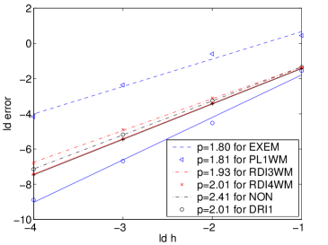
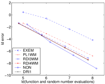
Figure 1: Orders of convergence and computational effort per simulation path versus precision for SDE (34).

As a second example, a multi-dimensional SDE with initial value $X(0)=(1,1)^{T}$ and noncommutative noise driven by a $2$-dimensional Wiener process is considered [3]:

$$\begin{split}d\begin{pmatrix}X^{1}\\ X^{2}\end{pmatrix}&=\begin{pmatrix}-\frac{273}{512}&0\\ -\frac{1}{160}&-\frac{785}{512}+\frac{\sqrt{2}}{8}\end{pmatrix}\,\begin{pmatrix}X^{1}\\ X^{2}\end{pmatrix}\,dt+\begin{pmatrix}\frac{1}{4}X^{1}&\frac{1}{16}X^{1}\\ \frac{1-2\sqrt{2}}{4}X^{2}&\frac{1}{10}X^{1}+\frac{1}{16}X^{2}\end{pmatrix}\,d\begin{pmatrix}W^{1}\\ W^{2}\end{pmatrix}.\end{split}$$ (36)

Here, we are interested in the second moments which depend on both, the drift and the diffusion function (see [4] for details). Therefore, we choose $f(x)=(x^{1})^{2}$ and obtain

$$\begin{split}\operatorname{E}(f(X(t)))=\exp(-t)\,.\end{split}$$ (37)

We approximate $\operatorname{E}(f(X(t)))$ at $t=10$ by $M=8\cdot 10^{7}$ simulated trajectories with step sizes $2^{0},\ldots,2^{-3}$. The results for the schemes in consideration are presented in Table 3 and Figure 2. Here, the order of convergence is $1.72$ for EXEM, $2.32$ for PL1WM, $2.14$ for RDI3WM, $2.17$ for RDI4WM, $2.07$ for NON and order $2.17$ for our new scheme DRI1.

Table 3: Mean errors, empirical variances and confidence intervals for SDE (36).

	$h$	$\hat{\mu}$	$\hat{\sigma}_{\mu}^{2}$	$a$	$b$
EXEM	$2^{-0}$	-2.165E-05	1.678E-14	-2.169E-05	-2.160E-05
	$2^{-1}$	-7.684E-06	1.418E-14	-7.724E-06	-7.643E-06
	$2^{-2}$	-2.266E-06	1.501E-14	-2.308E-06	-2.224E-06
	$2^{-3}$	-6.078E-07	3.567E-14	-6.725E-07	-5.432E-07
PL1WM	$2^{-0}$	3.093E-05	9.082E-15	3.090E-05	3.097E-05
	$2^{-1}$	4.947E-06	1.085E-14	4.906E-06	4.987E-06
	$2^{-2}$	1.071E-06	5.886E-15	1.041E-06	1.101E-06
	$2^{-3}$	2.435E-07	4.652E-15	2.172E-07	2.699E-07
RDI3WM	$2^{-0}$	-1.092E-05	2.481E-15	-1.094E-05	-1.090E-05
	$2^{-1}$	-2.335E-06	8.234E-15	-2.370E-06	-2.299E-06
	$2^{-2}$	-5.143E-07	5.519E-15	-5.431E-07	-4.856E-07
	$2^{-3}$	-1.285E-07	4.581E-15	-1.546E-07	-1.023E-07
RDI4WM	$2^{-0}$	-9.312E-06	3.403E-15	-9.334E-06	-9.289E-06
	$2^{-1}$	-1.893E-06	8.765E-15	-1.929E-06	-1.857E-06
	$2^{-2}$	-4.096E-07	5.591E-15	-4.386E-07	-3.807E-07
	$2^{-3}$	-1.035E-07	4.597E-15	-1.297E-07	-7.724E-08
NON	$2^{-0}$	6.396E-06	1.588E-14	6.347E-06	6.445E-06
	$2^{-1}$	1.548E-06	1.266E-14	1.504E-06	1.591E-06
	$2^{-2}$	3.799E-07	6.172E-15	3.495E-07	4.102E-07
	$2^{-3}$	8.544E-08	4.713E-15	5.889E-08	1.120E-07
DRI1	$2^{-0}$	-9.391E-06	3.332E-15	-9.414E-06	-9.369E-06
	$2^{-1}$	-1.908E-06	8.710E-15	-1.944E-06	-1.872E-06
	$2^{-2}$	-4.127E-07	5.587E-15	-4.416E-07	-3.838E-07
	$2^{-3}$	-1.041E-07	4.597E-15	-1.304E-07	-7.792E-08

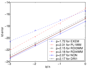
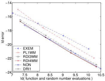
Figure 2: Orders of convergence and computational effort per simulation path versus precision for SDE (36).

Comparing the computational effort versus precision, in this example the schemes DRI1 and RDI4WM perform better than NON and RDI3WM and clearly better than EXEM and the Platen scheme.
Our last example is a nonlinear SDE with 10 Wiener processes,

$$dX(t)=X(t)\,dt+\frac{1}{10}\sqrt{X(t)+\frac{1}{2}}\,dW_{1}(t)+\frac{1}{15}\sqrt{X(t)+\frac{1}{4}}\,dW_{2}(t)$$ (38)

$$+\frac{1}{20}\sqrt{X(t)+\frac{1}{5}}\,dW_{3}(t)+\frac{1}{25}\sqrt{X(t)+\frac{1}{10}}\,dW_{4}(t)+\frac{1}{40}\sqrt{X(t)+\frac{1}{20}}\,dW_{5}(t)$$

$$+\frac{1}{25}\sqrt{X(t)+\frac{1}{2}}\,dW_{6}(t)+\frac{1}{20}\sqrt{X(t)+\frac{1}{4}}\,dW_{7}(t)+\frac{1}{15}\sqrt{X(t)+\frac{1}{5}}\,dW_{8}(t)$$

$$+\frac{1}{20}\sqrt{X(t)+\frac{1}{10}}\,dW_{9}(t)+\frac{1}{25}\sqrt{X(t)+\frac{1}{20}}\,dW_{10}(t),\qquad X(0)=1.$$

Here, we consider the fourth moment, i. e., $f(x)=x^{4}$, and obtain

$$\operatorname{E}(f(X(t)))=\frac{\scriptstyle 4625768169}{\scriptstyle 73570420483600}-\frac{\scriptstyle 2998776077847}{\scriptstyle 113706563209000}e^{\frac{731453}{360000}t}+\frac{\scriptstyle 80235120932849}{\scriptstyle 78178246418000}e^{\frac{251453}{60000}t}.$$ (39)

We approximate $E(f(X(t)))$ at $t=1$ by $M=2\cdot 10^{7}$ simulated trajectories with step sizes $2^{0},\dots,2^{-3}$ and obtain the results presented in Table 4 and Figure 3. The order of convergence is $1.30$ for EXEM, $1.60$ for PL1WM, $1.86$ for RDI3WM, $1.91$ for RDI4WM, $1.62$ for NON and $2.02$ for DRI1. If we take the computational effort into account, we see that DRI1 performs impressively better than all other schemes, which is what we expected for high numbers of Wiener processes.

Table 4: Mean errors, empirical variances and confidence intervals for SDE (38).

	$h$	$\hat{\mu}$	$\hat{\sigma}_{\mu}^{2}$	$a$	$b$
EXEM	$2^{0}$	-2.793E+01	7.005E-04	-2.794E+01	-2.792E+01
	$2^{-1}$	-1.420E+01	2.521E-03	-1.421E+01	-1.418E+01
	$2^{-2}$	-5.658E+00	7.216E-03	-5.687E+00	-5.629E+00
	$2^{-3}$	-1.872E+00	1.040E-02	-1.907E+00	-1.837E+00
PL1WM	$2^{-0}$	-2.266E+01	1.183E-03	-2.268E+01	-2.265E+01
	$2^{-1}$	-9.218E+00	1.954E-03	-9.234E+00	-9.203E+00
	$2^{-2}$	-2.965E+00	4.226E-03	-2.987E+00	-2.942E+00
	$2^{-3}$	-8.294E-01	4.294E-03	-8.519E-01	-8.070E-01
RDI3WM	$2^{0}$	-1.019E+01	1.727E-03	-1.021E+01	-1.018E+01
	$2^{-1}$	-3.161E+00	2.324E-03	-3.177E+00	-3.144E+00
	$2^{-2}$	-8.582E-01	4.494E-03	-8.812E-01	-8.353E-01
	$2^{-3}$	-2.136E-01	4.373E-03	-2.363E-01	-1.910E-01
RDI4WM	$2^{0}$	-9.546E+00	1.930E-03	-9.561E+00	-9.531E+00
	$2^{-1}$	-2.824E+00	2.436E-03	-2.840E+00	-2.807E+00
	$2^{-2}$	-7.398E-01	4.557E-03	-7.629E-01	-7.167E-01
	$2^{-3}$	-1.791E-01	4.392E-03	-2.017E-01	-1.564E-01
NON	$2^{0}$	5.331E+00	4.219E-03	5.309E+00	5.353E+00
	$2^{-1}$	1.883E+00	5.097E-03	1.858E+00	1.907E+00
	$2^{-2}$	5.877E-01	2.975E-03	5.690E-01	6.063E-01
	$2^{-3}$	1.850E-01	2.832E-03	1.668E-01	2.033E-01
DRI1	$2^{0}$	-9.465E+00	1.103E-03	-9.476E+00	-9.453E+00
	$2^{-1}$	-2.743E+00	3.070E-03	-2.762E+00	-2.724E+00
	$2^{-2}$	-6.834E-01	2.531E-03	-7.006E-01	-6.662E-01
	$2^{-3}$	-1.425E-01	2.704E-03	-1.603E-01	-1.247E-01

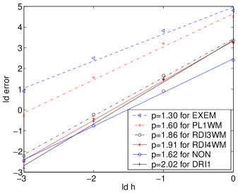
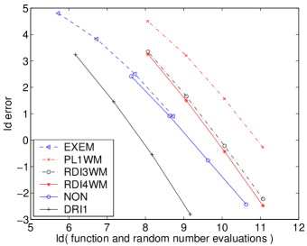
Figure 3: Orders of convergence and computational effort per simulation path versus precision for SDE (38).

6 Conclusion

In the present work, a full classification of the coefficients for a new class of efficient explicit SRK methods of order $(1,1)$ for $s=1$ and order $(2,1)$ for $s=2$ stages as well as for order $(2,2)$ with $s=3$ stages is calculated. Based on this classification, coefficients for an extension of the deterministic RK32 scheme to the stochastic case with minimized error constant are given. For three examples, this scheme is finally compared with the order two Platen and extrapolated Euler scheme, the schemes RDI3WM and RDI4WM and NON. It turns out that the new developed scheme performs very well and especially much better than all other schemes in the case of a high number of Wiener processes.

References

- [1] K. Burrage and P. M. Burrage, High strong order explicit Runge-Kutta methods for stochastic ordinary differential equations, Appl. Numer. Math., 22, No. 1-3, (1996) 81–101.
- [2] J. C. Butcher, Numerical methods for ordinary differential equations, John Wiley & Sons, West Sussex, 2003.
- [3] K. Debrabant, A. Rößler, Classification of stochastic Runge-Kutta methods for the weak approximation of stochastic differential equations, Math. Comput. Simulation 77 (4) (2008) 408–420.
- [4] P. E. Kloeden and E. Platen, Numerical solution of stochastic differential equations (Applications of Mathematics 23, Springer-Verlag, Berlin, 1999).
- [5] Y. Komori, Weak second-order stochastic Runge-Kutta methods for non-commutative stochastic differential equations, J. Comput. Appl. Math. 206 (1) (2007) 158–173.
- [6] V. Mackevicius and J. Navikas, Second order weak Runge-Kutta type methods for Itô equations, Math. Comput. Simul., Vol. 57, No. 1–2, (2001), 29–34.
- [7] G. N. Milstein, Numerical integration of stochastic differential equations, Kluwer Academic Publishers, Dordrecht, 1995.
- [8] A. Rößler, Rooted tree analysis for order conditions of stochastic Runge-Kutta methods for the weak approximation of stochastic differential equations, Stochastic Anal. Appl. Vol. 24, No. 1, (2006), 97–134.
- [9] A. Rößler, Runge-Kutta methods for Itô stochastic differential equations with scalar noise, BIT, Vol. 46, No. 1, (2006), 97–110.
- [10] A. Rößler, Second order Runge–Kutta methods for Itô stochastic differential equations, SIAM J. Numer. Anal., Vol. 47, No. 3, (2009), 1713–1738.
- [11] A. Rößler, Second order Runge–Kutta methods for Stratonovich stochastic differential equations, BIT, Vol. 47, No. 3, (2007), 657–680.
- [12] D. Talay and L. Tubaro, Expansion of the global error for numerical schemes solving stochastic differential equations, Stochastic Anal. Appl., Vol. 8, No. 4, (1990),94–120.
- [13] A. Tocino and J. Vigo-Aguiar, Weak second order conditions for stochastic Runge-Kutta methods, SIAM J. Sci. Comput., Vol. 24, No. 2, (2002), 507–523.