22institutetext: Aalto University Metsähovi Radio Observatory and Dept of Radio Science and Engineering, P.O. Box 13000, FI-00076 AALTO, Finland
33institutetext: African Institute for Mathematical Sciences, 6-8 Melrose Road, Muizenberg, Cape Town, South Africa
44institutetext: Agenzia Spaziale Italiana Science Data Center, Via del Politecnico snc, 00133, Roma, Italy
55institutetext: Agenzia Spaziale Italiana, Viale Liegi 26, Roma, Italy
66institutetext: Astrophysics Group, Cavendish Laboratory, University of Cambridge, J J Thomson Avenue, Cambridge CB3 0HE, U.K.
77institutetext: Astrophysics & Cosmology Research Unit, School of Mathematics, Statistics & Computer Science, University of KwaZulu-Natal, Westville Campus, Private Bag X54001, Durban 4000, South Africa
88institutetext: CITA, University of Toronto, 60 St. George St., Toronto, ON M5S 3H8, Canada
99institutetext: CNRS, IRAP, 9 Av. colonel Roche, BP 44346, F-31028 Toulouse cedex 4, France
1010institutetext: California Institute of Technology, Pasadena, California, U.S.A.
1111institutetext: Centre for Theoretical Cosmology, DAMTP, University of Cambridge, Wilberforce Road, Cambridge CB3 0WA, U.K.
1212institutetext: Centro de Estudios de Física del Cosmos de Aragón (CEFCA), Plaza San Juan, 1, planta 2, E-44001, Teruel, Spain
1313institutetext: Computational Cosmology Center, Lawrence Berkeley National Laboratory, Berkeley, California, U.S.A.
1414institutetext: Consejo Superior de Investigaciones Científicas (CSIC), Madrid, Spain
1515institutetext: DSM/Irfu/SPP, CEA-Saclay, F-91191 Gif-sur-Yvette Cedex, France
1616institutetext: DTU Space, National Space Institute, Technical University of Denmark, Elektrovej 327, DK-2800 Kgs. Lyngby, Denmark
1717institutetext: Département de Physique Théorique, Université de Genève, 24, Quai E. Ansermet,1211 Genève 4, Switzerland
1818institutetext: Departamento de Física Fundamental, Facultad de Ciencias, Universidad de Salamanca, 37008 Salamanca, Spain
1919institutetext: Departamento de Física, Universidad de Oviedo, Avda. Calvo Sotelo s/n, Oviedo, Spain
2020institutetext: Department of Astronomy and Astrophysics, University of Toronto, 50 Saint George Street, Toronto, Ontario, Canada
2121institutetext: Department of Astrophysics/IMAPP, Radboud University Nijmegen, P.O. Box 9010, 6500 GL Nijmegen, The Netherlands
2222institutetext: Department of Electrical Engineering and Computer Sciences, University of California, Berkeley, California, U.S.A.
2323institutetext: Department of Physics & Astronomy, University of British Columbia, 6224 Agricultural Road, Vancouver, British Columbia, Canada
2424institutetext: Department of Physics and Astronomy, Dana and David Dornsife College of Letter, Arts and Sciences, University of Southern California, Los Angeles, CA 90089, U.S.A.
2525institutetext: Department of Physics and Astronomy, University College London, London WC1E 6BT, U.K.
2626institutetext: Department of Physics, Florida State University, Keen Physics Building, 77 Chieftan Way, Tallahassee, Florida, U.S.A.
2727institutetext: Department of Physics, Gustaf Hällströmin katu 2a, University of Helsinki, Helsinki, Finland
2828institutetext: Department of Physics, Princeton University, Princeton, New Jersey, U.S.A.
2929institutetext: Department of Physics, University of Alberta, 11322-89 Avenue, Edmonton, Alberta, T6G 2G7, Canada
3030institutetext: Department of Physics, University of California, One Shields Avenue, Davis, California, U.S.A.
3131institutetext: Department of Physics, University of California, Santa Barbara, California, U.S.A.
3232institutetext: Department of Physics, University of Illinois at Urbana-Champaign, 1110 West Green Street, Urbana, Illinois, U.S.A.
3333institutetext: Dipartimento di Fisica e Astronomia G. Galilei, Università degli Studi di Padova, via Marzolo 8, 35131 Padova, Italy
3434institutetext: Dipartimento di Fisica e Scienze della Terra, Università di Ferrara, Via Saragat 1, 44122 Ferrara, Italy
3535institutetext: Dipartimento di Fisica, Università La Sapienza, P. le A. Moro 2, Roma, Italy
3636institutetext: Dipartimento di Fisica, Università degli Studi di Milano, Via Celoria, 16, Milano, Italy
3737institutetext: Dipartimento di Fisica, Università degli Studi di Trieste, via A. Valerio 2, Trieste, Italy
3838institutetext: Dipartimento di Fisica, Università di Roma Tor Vergata, Via della Ricerca Scientifica, 1, Roma, Italy
3939institutetext: Discovery Center, Niels Bohr Institute, Blegdamsvej 17, Copenhagen, Denmark
4040institutetext: Dpto. Astrofísica, Universidad de La Laguna (ULL), E-38206 La Laguna, Tenerife, Spain
4141institutetext: European Space Agency, ESAC, Planck Science Office, Camino bajo del Castillo, s/n, Urbanización Villafranca del Castillo, Villanueva de la Cañada, Madrid, Spain
4242institutetext: European Space Agency, ESTEC, Keplerlaan 1, 2201 AZ Noordwijk, The Netherlands
4343institutetext: Helsinki Institute of Physics, Gustaf Hällströmin katu 2, University of Helsinki, Helsinki, Finland
4444institutetext: INAF - Osservatorio Astronomico di Padova, Vicolo dell’Osservatorio 5, Padova, Italy
4545institutetext: INAF - Osservatorio Astronomico di Roma, via di Frascati 33, Monte Porzio Catone, Italy
4646institutetext: INAF - Osservatorio Astronomico di Trieste, Via G.B. Tiepolo 11, Trieste, Italy
4747institutetext: INAF Istituto di Radioastronomia, Via P. Gobetti 101, 40129 Bologna, Italy
4848institutetext: INAF/IASF Bologna, Via Gobetti 101, Bologna, Italy
4949institutetext: INAF/IASF Milano, Via E. Bassini 15, Milano, Italy
5050institutetext: INFN, Sezione di Bologna, Via Irnerio 46, I-40126, Bologna, Italy
5151institutetext: INFN, Sezione di Roma 1, Università di Roma Sapienza, Piazzale Aldo Moro 2, 00185, Roma, Italy
5252institutetext: IPAG: Institut de Planétologie et d’Astrophysique de Grenoble, Université Joseph Fourier, Grenoble 1 / CNRS-INSU, UMR 5274, Grenoble, F-38041, France
5353institutetext: IUCAA, Post Bag 4, Ganeshkhind, Pune University Campus, Pune 411 007, India
5454institutetext: Imperial College London, Astrophysics group, Blackett Laboratory, Prince Consort Road, London, SW7 2AZ, U.K.
5555institutetext: Infrared Processing and Analysis Center, California Institute of Technology, Pasadena, CA 91125, U.S.A.
5656institutetext: Institut Néel, CNRS, Université Joseph Fourier Grenoble I, 25 rue des Martyrs, Grenoble, France
5757institutetext: Institut Universitaire de France, 103, bd Saint-Michel, 75005, Paris, France
5858institutetext: Institut d’Astrophysique Spatiale, CNRS (UMR8617) Université Paris-Sud 11, Bâtiment 121, Orsay, France
5959institutetext: Institut d’Astrophysique de Paris, CNRS (UMR7095), 98 bis Boulevard Arago, F-75014, Paris, France
6060institutetext: Institute for Space Sciences, Bucharest-Magurale, Romania
6161institutetext: Institute of Astronomy and Astrophysics, Academia Sinica, Taipei, Taiwan
6262institutetext: Institute of Astronomy, University of Cambridge, Madingley Road, Cambridge CB3 0HA, U.K.
6363institutetext: Institute of Theoretical Astrophysics, University of Oslo, Blindern, Oslo, Norway
6464institutetext: Instituto de Astrofísica de Canarias, C/Vía Láctea s/n, La Laguna, Tenerife, Spain
6565institutetext: Instituto de Física de Cantabria (CSIC-Universidad de Cantabria), Avda. de los Castros s/n, Santander, Spain
6666institutetext: Jet Propulsion Laboratory, California Institute of Technology, 4800 Oak Grove Drive, Pasadena, California, U.S.A.
6767institutetext: Jodrell Bank Centre for Astrophysics, Alan Turing Building, School of Physics and Astronomy, The University of Manchester, Oxford Road, Manchester, M13 9PL, U.K.
6868institutetext: Kavli Institute for Cosmology Cambridge, Madingley Road, Cambridge, CB3 0HA, U.K.
6969institutetext: LAL, Université Paris-Sud, CNRS/IN2P3, Orsay, France
7070institutetext: LERMA, CNRS, Observatoire de Paris, 61 Avenue de l’Observatoire, Paris, France
7171institutetext: Laboratoire AIM, IRFU/Service d’Astrophysique - CEA/DSM - CNRS - Université Paris Diderot, Bât. 709, CEA-Saclay, F-91191 Gif-sur-Yvette Cedex, France
7272institutetext: Laboratoire Traitement et Communication de l’Information, CNRS (UMR 5141) and Télécom ParisTech, 46 rue Barrault F-75634 Paris Cedex 13, France
7373institutetext: Laboratoire de Physique Subatomique et de Cosmologie, Université Joseph Fourier Grenoble I, CNRS/IN2P3, Institut National Polytechnique de Grenoble, 53 rue des Martyrs, 38026 Grenoble cedex, France
7474institutetext: Laboratoire de Physique Théorique, Université Paris-Sud 11 & CNRS, Bâtiment 210, 91405 Orsay, France
7575institutetext: Lawrence Berkeley National Laboratory, Berkeley, California, U.S.A.
7676institutetext: Max-Planck-Institut für Astrophysik, Karl-Schwarzschild-Str. 1, 85741 Garching, Germany
7777institutetext: McGill Physics, Ernest Rutherford Physics Building, McGill University, 3600 rue University, Montréal, QC, H3A 2T8, Canada
7878institutetext: MilliLab, VTT Technical Research Centre of Finland, Tietotie 3, Espoo, Finland
7979institutetext: Mullard Space Science Laboratory, University College London, Surrey RH5 6NT, U.K.
8080institutetext: National University of Ireland, Department of Experimental Physics, Maynooth, Co. Kildare, Ireland
8181institutetext: Niels Bohr Institute, Blegdamsvej 17, Copenhagen, Denmark
8282institutetext: Observational Cosmology, Mail Stop 367-17, California Institute of Technology, Pasadena, CA, 91125, U.S.A.
8383institutetext: Optical Science Laboratory, University College London, Gower Street, London, U.K.
8484institutetext: SB-ITP-LPPC, EPFL, CH-1015, Lausanne, Switzerland
8585institutetext: SISSA, Astrophysics Sector, via Bonomea 265, 34136, Trieste, Italy
8686institutetext: School of Physics and Astronomy, Cardiff University, Queens Buildings, The Parade, Cardiff, CF24 3AA, U.K.
8787institutetext: School of Physics and Astronomy, University of Nottingham, Nottingham NG7 2RD, U.K.
8888institutetext: Space Sciences Laboratory, University of California, Berkeley, California, U.S.A.
8989institutetext: Special Astrophysical Observatory, Russian Academy of Sciences, Nizhnij Arkhyz, Zelenchukskiy region, Karachai-Cherkessian Republic, 369167, Russia
9090institutetext: Stanford University, Dept of Physics, Varian Physics Bldg, 382 Via Pueblo Mall, Stanford, California, U.S.A.
9191institutetext: Sub-Department of Astrophysics, University of Oxford, Keble Road, Oxford OX1 3RH, U.K.
9292institutetext: Theory Division, PH-TH, CERN, CH-1211, Geneva 23, Switzerland
9393institutetext: UPMC Univ Paris 06, UMR7095, 98 bis Boulevard Arago, F-75014, Paris, France
9494institutetext: Université de Toulouse, UPS-OMP, IRAP, F-31028 Toulouse cedex 4, France
9595institutetext: University of Granada, Departamento de Física Teórica y del Cosmos, Facultad de Ciencias, Granada, Spain
9696institutetext: Warsaw University Observatory, Aleje Ujazdowskie 4, 00-478 Warszawa, Poland
Planck 2013 results. XXVI. Background geometry and topology of the Universe
The new cosmic microwave background (CMB) temperature maps from Planck provide the highest-quality full-sky view of the surface of last scattering available to date. This allows us to detect possible departures from the standard model of a globally homogeneous and isotropic cosmology on the largest scales. We search for correlations induced by a possible non-trivial topology with a fundamental domain intersecting, or nearly intersecting, the last scattering surface (at comoving distance ), both via a direct search for matched circular patterns at the intersections and by an optimal likelihood search for specific topologies. For the latter we consider flat spaces with cubic toroidal (T3), equal-sided chimney (T2) and slab (T1) topologies, three multi-connected spaces of constant positive curvature (dodecahedral, truncated cube and octahedral) and two compact negative-curvature spaces. These searches yield no detection of the compact topology with the scale below the diameter of the last scattering surface. For most compact topologies studied the likelihood maximized over the orientation of the space relative to the observed map shows some preference for multi-connected models just larger than the diameter of the last scattering surface. Since this effect is also present in simulated realizations of isotropic maps, we interpret it as the inevitable alignment of mild anisotropic correlations with chance features in a single sky realization; such a feature can also be present, in milder form, when the likelihood is marginalized over orientations. Thus marginalized, the limits on the radius of the largest sphere inscribed in topological domain (at log-likelihood-ratio relative to a simply-connected flat Planck best-fit model) are: in a flat Universe, for the T3 cubic torus; for the T2 chimney; for the T1 slab; and in a positively curved Universe, for the dodecahedral space; for the truncated cube; and for the octahedral space. The limit for a wider class of topologies, i.e., those predicting matching pairs of back-to-back circles, among them tori and the three spherical cases listed above, coming from the matched-circles search is at 99 % confidence level. Similar limits apply to a wide, although not exhaustive, range of topologies.
We also perform a Bayesian search for an anisotropic global Bianchi VIIh geometry. In the non-physical setting where the Bianchi cosmology is decoupled from the standard cosmology, Planck data favour the inclusion of a Bianchi component with a Bayes factor of at least 1.5 units of log-evidence. Indeed, the Bianchi pattern is quite efficient at accounting for some of the large-scale anomalies found in Planck data. However, the cosmological parameters that generate this pattern are in strong disagreement with those found from CMB anisotropy data alone. In the physically motivated setting where the Bianchi parameters are coupled and fitted simultaneously with the standard cosmological parameters, we find no evidence for a Bianchi VIIh cosmology and constrain the vorticity of such models to (95 % confidence level).
Key Words.:
cosmology: observations — cosmic background radiation — cosmological parameters — Gravitation — Methods: data analysis — Methods: statistical1 Introduction
This paper, one of a set of papers associated with the 2013 release of data from the Planck111Planck (http://www.esa.int/Planck) is a project of the European Space Agency (ESA) with instruments provided by two scientific consortia funded by ESA member states (in particular the lead countries France and Italy), with contributions from NASA (USA) and telescope reflectors provided by a collaboration between ESA and a scientific consortium led and funded by Denmark. mission (Planck Collaboration I 2014), describes the use of Planck data to limit departures from the global isotropy and homogeneity of spacetime. We will use Planck’s measurements of the cosmic microwave background (CMB) to assess the properties of anisotropic geometries (i.e., Bianchi models) and non-trivial topologies (e.g., the torus). The simplest models of spacetime are globally isotropic and simply connected. Although both are supported by both local observations and previous CMB observations, without a fundamental theory of the birth of the Universe, observational constraints on departures from global isotropy are necessary. General Relativity itself places no restrictions upon the topology of the Universe, as was recognised very early on (e.g., de Sitter 1917); most proposed theories of quantum gravity predict topology-change in the early Universe which could be visible at large scales today.
The Einstein field equations relate local properties of the curvature to the matter content in spacetime. By themselves they do not restrict the global properties of the space, allowing a universe with a given local geometry to have various global topologies. Friedmann–Robertson-–Walker (FRW) models of the universe observed to have the same average local properties everywhere still have freedom to describe quite different spaces at large scales. Perhaps the most remarkable possibility is that a vanishing or negative local curvature () does not necessarily mean that our Universe is infinite. Indeed we can still be living in a universe of finite volume due to the global topological multi-connectivity of space, even if described by the flat or hyperbolic FRW solutions. In particular, quantum fluctuations can produce compact spaces of constant curvature, both flat (e.g., Zeldovich & Starobinskii 1984) and curved (e.g., Coule & Martin 2000; Linde 2004), within the inflationary scenario.
The primary CMB anisotropy alone is incapable of constraining curvature due to the well-known geometrical degeneracy which produces identical small-scale fluctuations when the recombination sound speed, initial fluctuations, and comoving distance to the last scattering surface are kept constant (e.g., Bond et al. 1997; Zaldarriaga & Seljak 1997; Stompor & Efstathiou 1999). The present results from Planck (Planck Collaboration XVI 2014) can therefore place restrictive constraints on the curvature of the Universe only when considering secondary anisotropies or non-CMB data: at 95 %, considering CMB primary anisotropy and lensing from Planck (in the natural units with we use throughout). This is equivalent to constraints on the radius of curvature for positive curvature () and for negative curvature (). CMB primary anisotropy alone gives limits on roughly a factor of two less restrictive (and strongly dependent on priors).
Thus, the global nature of the Universe we live in is still an open question and studying the observational effects of a possible finite universe is one way to address it. With topology not affecting local mean properties that are found to be well described by FRW parameters, its main observational effect is in setting boundary conditions on perturbation modes that can be excited and developed into the structure that we observe. Studying structure on the last scattering surface is the best-known way to probe the global organisation of our Universe and the CMB provides the most detailed and best understood dataset for this purpose.
We can also relax assumptions about the global structure of spacetime by allowing anisotropy about each point in the Universe. This yields more general solutions to Einstein’s field equations, leading to the so-called Bianchi cosmologies. For small anisotropy, as demanded by current observations, linear perturbation about the standard FRW model may be applied. A universal shear and rotation induce a characteristic subdominant, deterministic signature in the CMB, which is embedded in the usual stochastic anisotropies. The deterministic CMB temperature fluctuations that result in the homogenous Bianchi models were first examined by Collins & Hawking (1973) and Barrow et al. (1985) (and subsequently Barrow 1986), however no dark energy component was included as it was not considered plausible at the time. More recently, Jaffe et al. (2006c), and independently Bridges et al. (2007), extended these solutions for the open and flat Bianchi VIIh models to include cosmologies with dark energy. It is these solutions to Bianchi VIIh models that we study in the current article. More accurate solutions were since derived by Pontzen & Challinor (2007), Pontzen (2009) and Pontzen & Challinor (2011), where recombination is treated in a more sophisticated manner and reionisation is supported. Furthermore, we note that in these works (Pontzen & Challinor 2007; Pontzen 2009; Pontzen & Challinor 2011) the induced CMB polarisation contributions that arise in Bianchi models have also been derived, although here focus is given to temperature contributions.
In this paper, we will explicitly consider models of global topology and anisotropy. In a chaotic inflation scenario, however, our post-inflationary patch might exhibit large-scale local topological features (“handles” and “holes”) the can mimic a global multiply-connected topology in our observable volume. Similarly, it might also have residual shear or rotation which could mimic the properties of a global Bianchi spacetime.
Planck’s ability to discriminate and remove large-scale astrophysical foregrounds (Planck Collaboration XII 2014) reduces the systematic error budget associated with measurements of the CMB sky significantly. Planck data therefore allow refined limits on the scale of the topology and the presence of anisotropy. Moreover, previous work in this field has been done by a wide variety of authors using a wide variety of data (e.g., COBE, WMAP 1-year, 3-year, 5-year, etc.) and in this work we perform a coherent analysis.
In Sect. 2, we discuss previous attempts to limit the topology and global isotropy of the Universe. In Sect. 3 we discuss the signals induced in topologically non-trivial and Bianchi universes. In Sect. 4 the Planck data we use in the analysis are presented, and in Sect. 5 the methods we have developed to detect those signals are discussed. We apply those methods in Sect. 6 and discuss the results in Sect. 7.
2 Previous results
The first searches for non-trivial topology on cosmic scales looked for repeated patterns or individual objects in the distribution of galaxies (Sokolov & Shvartsman 1974; Fang & Sato 1983; Fagundes & Wichoski 1987; Lehoucq et al. 1996; Roukema 1996; Weatherley et al. 2003; Fujii & Yoshii 2011). The last scattering surface from which the CMB is released represents the most distant source of photons in the Universe, and hence the largest scales with which we could probe the topology of the Universe. This first became possible with the DMR instrument on the COBE satellite (Bennett et al. 1996): various searches found no evidence for non-trivial topologies (e.g., Starobinskij 1993; Sokolov 1993; Stevens et al. 1993; de Oliveira-Costa & Smoot 1995; Levin et al. 1998; Bond et al. 1998, 2000b; Rocha et al. 2004; but see also Roukema 2000b, a), but sparked the creation of robust statistical tools, along with greater care in the enumeration of the possible topologies for a given geometry (see, for example, Lachieze-Rey & Luminet 1995 and Levin 2002 for reviews). With data from the WMAP satellite (Jarosik et al. 2011), these theoretical and observational tools were applied to a high-quality dataset for the first time. Luminet et al. (2003) and Caillerie et al. (2007) claimed the low value of the low multipoles (compared to standard CDM cosmology) as evidence for missing large-scale power as predicted in a closed universe with a small fundamental domain (see also Aurich 1999; Aurich et al. 2004, 2005, 2006, 2008; Aurich & Lustig 2013; Lew & Roukema 2008; Roukema et al. 2008). However, searches in pixel space (Cornish et al. 2004; Key et al. 2007; Niarchou et al. 2004; Bielewicz & Riazuelo 2009; Dineen et al. 2005) and in harmonic space (Kunz et al. 2006) determined that this was an unlikely explanation for the low power. Bond et al. (1998, 2000a) and Riazuelo et al. (2004a, b) presented some of the mathematical formalism for the computation of the correlations induced by topology in a form suitable for use in cosmological calculations. Phillips & Kogut (2006) presented efficient algorithms for the computation of the correlation structure of the flat torus and applied it via a Bayesian formalism to the WMAP data; similar computations for a wider range of geometries were performed by Niarchou & Jaffe (2007).
These calculations used a variety of different vintages of the COBE and WMAP data, as well as a variety of different sky cuts (including the unmasked internal linear combination (ILC) map, not originally intended for cosmological studies). Nonetheless, none of the pixel-space calculations which took advantage of the full correlation structure induced by the topology found evidence for a multiply-connected topology with a fundamental domain within or intersecting the last scattering surface. Hence in this paper we will attempt to corroborate this earlier work and put the calculations on a consistent footing.
The open and flat Bianchi type VIIh models have been compared previously to both the COBE (Bunn et al. 1996; Kogut et al. 1997) and WMAP (Jaffe et al. 2005, 2006b) data, albeit ignoring dark energy, in order to place limits on the global rotation and shear of the Universe. A statistically significant correlation between one of the Bianchi VIIh models and the WMAP ILC map (Bennett et al. 2003) was first detected by Jaffe et al. (2005). However, it was noted that the parameters of this model are inconsistent with standard constraints. Nevertheless, when the WMAP ILC map was “corrected” for the best-fit Bianchi template, some of the so-called “anomalies” reported in WMAP data disappear (Jaffe et al. 2005, 2006b; Cayón et al. 2006; McEwen et al. 2006). A modified template fitting technique was performed by Land & Magueijo (2006) and, although a statistically significant template fit was not reported, the corresponding “corrected” WMAP data were again free of many large scale “anomalies”. Subsequently, Ghosh et al. (2007) used the bipolar power spectrum of WMAP data to constrain the amplitude of any Bianchi component in the CMB. Due to the renewed interest in Bianchi models, solutions to the CMB temperature fluctuations induced in Bianchi VIIh models when incorporating dark energy were since derived by Jaffe et al. (2006c) and Bridges et al. (2007). Nevertheless, the cosmological parameters of the Bianchi template embedded in WMAP data in this setting remain inconsistent with constraints from the CMB alone (Jaffe et al. 2006a, c). Furthermore, Pontzen & Challinor (2007) compared the polarisation power spectra of the best-fit Bianchi VIIh model found by Jaffe et al. (2006a) with the WMAP 3-year data (Page et al. 2007) and also concluded that the model could be ruled out since it produced greater polarization than observed in the WMAP data. A Bayesian analysis of Bianchi VIIh models was performed by Bridges et al. (2007) using WMAP ILC data to explore the joint cosmological and Bianchi parameter space via Markov chain Monte Carlo sampling, where it was again determined that the parameters of the resulting Bianchi cosmology were inconsistent with standard constraints. In a following study by Bridges et al. (2008) it was suggested that the CMB “cold spot” (Vielva et al. 2004; Cruz et al. 2006; Vielva 2010) could be driving evidence for a Bianchi component. Recently, this Bayesian analysis has been revisited by McEwen et al. (2013) to handle partial-sky observations and to use nested sampling methods (Skilling 2004; Feroz & Hobson 2008; Feroz et al. 2009). McEwen et al. (2013) conclude that WMAP 9-year temperature data do not favour Bianchi VIIh cosmologies over CDM.
3 CMB correlations in anisotropic and multiply-connected universes
3.1 Topology
All FRW models can describe multi-connected universes. In the case of flat space, there are a finite number of compactifications, the simplest of which are those of the torus. All of them have continuous parameters that describe the length of periodicity in some or all directions (e.g., Riazuelo et al. 2004b). In a space of constant non-zero curvature the situation is notably different — the presence of a length scale (the curvature radius ) precludes topological compactification at an arbitrary scale. The size of the space must now reflect its curvature, linking topological properties to . In the case of hyperbolic spacetimes, the list of possible compact spaces of constant negative curvature is still infinite, but discrete (Thurston 1982), while in the positive curvature spherical space there is only a finite set of well-proportioned possibilities (i.e., those with roughly comparable sizes in all directions; there are also the countably infinite lens and prism topologies) for a multi-connected space (e.g., Gausmann et al. 2001; Riazuelo et al. 2004a).
The effect of topology is equivalent to considering the full simply-connected three-dimensional spatial slice of the spacetime (known as the covering space) as being filled with repetitions of a shape which is finite in some or all directions (the fundamental domain) — by analogy with the two-dimensional case, we say that the fundamental domain tiles the covering space. For the flat and hyperbolic geometries, there are infinite copies of the fundamental domain; for the spherical geometry, with a finite volume, there is a finite number of tiles. Physical fields repeat their configuration in every tile, and thus can be viewed as defined on the covering space but subject to periodic boundary conditions. Topological compactification always break isotropy, and for some topologies also the global homogeneity of physical fields. Positively curved and flat spaces studied in this paper are homogeneous, however hyperbolic multi-connected spaces are never homogeneous.
| Size | Spherical | Hyperbolic | |||||
|---|---|---|---|---|---|---|---|
| Dodecahedral | Truncated Cube | Octahedral | m004(,1) | v3543(2,3) | |||
| 0.16 | 0.41 | 0.82 | 0.98 | 6.45 | |||
| 0.31 () | 0.39 () | 0.45 | 0.54 | 0.89 | |||
| 0.37 | 0.56 | 0.56 | 0.64 | 1.22 | |||
| 0.40 | 0.58 | 0.79 () | 0.75 | 1.33 | |||
The primary observable effect of a multi-connected universe is the existence of directions in which light could circumnavigate the space in cosmological time more than once, i.e., the radial distance to the surface of last scattering exceeds the size of the universe. In these cases, the surface of last scattering can intersect the (notional) edge of a fundamental domain. At this intersection, we can view the same spacetime event from multiple directions — conversely, it appears in different directions when observed from a single point.
Thus, temperature perturbations in one direction, , become correlated with those in another direction by an amount that differs from the usual isotropic correlation function , where denotes the angle between and . Considering a pixelized map, this induces a correlation matrix which depends on quantities other than the angular distance between pixels and . This break from statistical isotropy can therefore be used to constrain topological models. Hence, we need to calculate the pixel-space correlation matrix or its equivalent in harmonic space.
In this paper we consider the following topologies using the likelihood method: a) toroidal flat models with equal-length compactification size in three directions, denoted ;222In a slight abuse of notation, the lengths will be given in units of in , but in physical units elsewhere. b) toroidal flat models with different compactification lengths, parametrized by , denoted ; c) three major types of single-action positively curved spherical manifolds with dodecahedral, truncated cubical and octahedral fundamental domains (, , compactification groups correspondingly, see Gausmann et al. 2001); and d) two sample negative curvature hyperbolic spaces, m004(,1) being one of the smallest known compact hyperbolic spaces as well as the relatively large v3543(2,3).333The nomenclature for hyperbolic spaces follows J. Weeks’ census, as incorporated in the freely available SnapPea software, http://www.geometrygames.org/SnapPea; see also Thurston & Levy (1997). Scales of fundamental domains of compactified curved spaces are fixed in the units of curvature and are summarised in Table 1, where we quote the volume , radius of the largest sphere that can be inscribed in the domain (equal to the distance to the nearest face from the origin of the domain), the smallest sphere in which the domain can be inscribed (equal to the distance to the farthest vertex), and the intermediate scale that is taken to be the distance to the edges for spherical spaces and the “spine” distance for hyperbolic topologies. For the cubic torus with edge length , these lengths are , and . The ratio is a good indicator of the shape of the fundamental domain. Note that when is less than , multiple images on large scales are not present, although the correlation matrix is still modified versus the singly-connected limit. The effects of topology usually become strong when exceeds the intermediate ; conversely, for flat and nearly-flat geometries, there are limits to the allowed topologies (Mota et al. 2011).
A much wider class of topologies is explicitly constrained using the matched circles method. As discussed in Sect. 5.1, because of computational limitations we restrict our analysis to pairs of circles centered around antipodal points, so called back-to-back circles. Thus, we can constrain all topologies predicting pairs of such circles. The strongest constraints are imposed on topologies predicting back-to-back circles in all directions i.e., all the single action manifolds, among them tori of any shape and the three spherical cases considered explicitly in the likelihood analysis. Weaker constraints are imposed on topologies with all back-to-back circles centred on a great circle of the celestial sphere such as half-turn, quarter-turn, third-turn and sixth-turn spaces, as well as Klein and chimney spaces. The statistic can also constrain the multi-connected spaces predicting one pair of antipodal matching circles such as Klein or chimney spaces with horizontal flip, vertical flip or half-turn and slab space translated without screw motion. Other topologies catalogued in Riazuelo et al. (2004b) are not constrained by this analysis: the Hantzsche-Wendt space; the chimney space with half-turn and flip; the generic slab space; the slab space with flip; spherical manifolds with double and linked action; and all the hyperbolic topologies including those two cases considered using the likelihood method.
3.1.1 Computing correlation matrices
The CMB temperature pixel-pixel correlation matrix is defined as the ensemble-average product of the temperature at two different pixels:
| (1) |
It can be calculated as a double radial integral of the ensemble average of the product of the source functions that describe the transport of photons through the universe from the last scattering surface to the observer:
| (2) |
where and are unit vectors that point at pixels and on the sky, and and are proper distances along radial rays pointing towards the last scattering surface.
Two techniques have been developed to compute the CMB correlation function for multiply-connected universes. In one approach, one constructs the orthonormal set of basis functions that satisfy the boundary conditions imposed by compactification (eigenfunctions of the Laplacian operator furnish such a basis), and assembles the spatial correlation function of the source from such a basis (Cornish & Spergel 1999; Lehoucq et al. 2002). In the other approach, one applies the method of images to create the compactified version of from the one computed on the universal covering space by resumming the latter over the images of the 3D spatial positions (Bond et al. 1998, 2000a, 2000b):
| (3) |
where the superscripts and refer to the quantity in the multiply-connected space and its universal cover, respectively. The tilde refers to the need for sum regularization in the models with an infinite set of images, e.g., hyperbolic and flat toroidal ones. is the discrete subgroup of motions which defines the multiply-connected space and is the spatial point on the universal cover obtained by the action of the motion on the point . Note that we can consider the location of one of the pixels as fixed and consider the action of on the other due to symmetry. This equation defines the action of on the source function itself, needed unless all the terms in the source function are scalar quantities (which is the case if one limits consideration to Sachs-Wolfe terms) when the action is trivial.
Both methods are general, but have practical considerations to take into account when one increases the pixel resolution. For computing up to the resolution corresponding to harmonic mode both methods have been tested and were found to work equally well. In this paper we employ both approaches.
The main effect of the compactification is that is no longer a function of the angular separation between the pixels and only, due to the lack of global isotropy. In harmonic space the two-point correlation function of the CMB is given by
| (4) |
where is the Kronecker delta symbol and are the spherical harmonic coefficients of the temperature on the sky when decomposed into the spherical harmonics by
| (5) |
Note that the two-point correlation function is no longer diagonal, nor is it -independent, as in an isotropic universe.
A flat universe provides an example when the eigenfunctions of the Laplacian are readily available in a set of plane waves. The topological compactification in the flat space discretizes the spectrum of the wavevector magnitudes and selects the subset of allowed directions. For example, for a toroidal universe the length of the fundamental cell needs to be an integer multiple of the wavelength of the modes. We therefore recover a discrete sum over modes for a triplet of integers, instead of an integral over ,
where is the radiation transfer function (e.g., Bond & Efstathiou 1987; Seljak 1996). We refer to the cubic torus with three equal sides as the T3 topology; it is also possible for the fundamental domain to be compact in only two spatial dimensions (e.g., the so-called T2 “chimney” space) or one (the T1 “slab”, similar to the “lens” spaces available in manifolds with constant positive curvature) in which case the sum is replaced by an integral in those directions. These models serve as approximations to modifications to the local topology of the global manifold (albeit on cosmological scales): for example, the chimney space can mimic a “handle” connecting different regions of an approximately flat manifold.
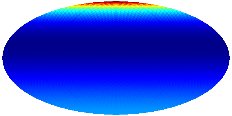
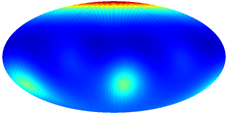
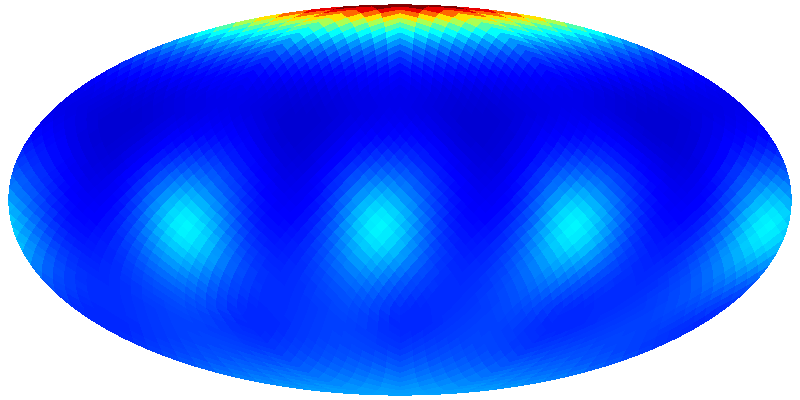
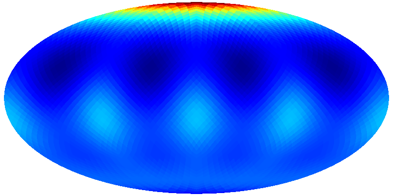
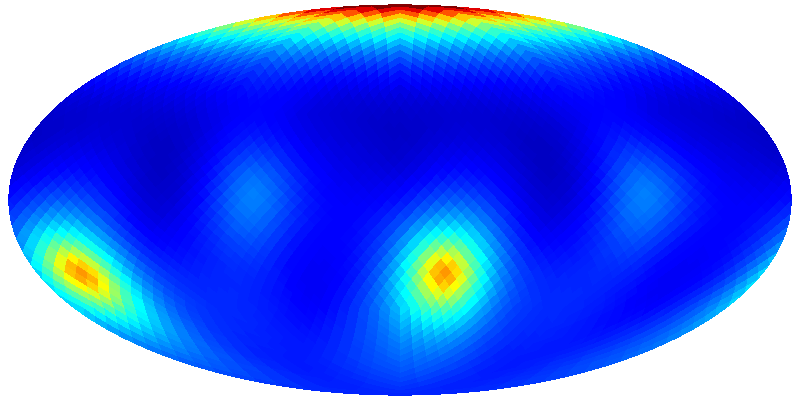
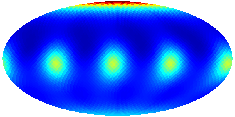
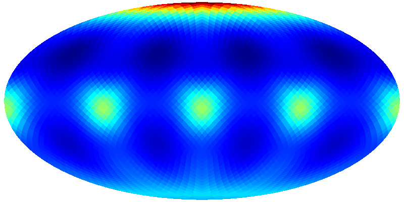
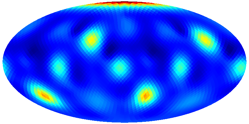
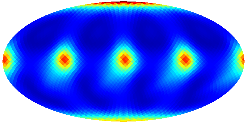
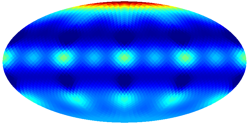
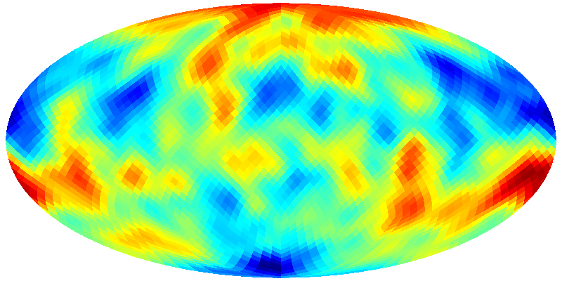
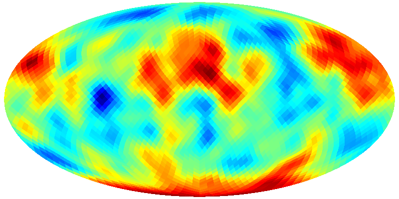
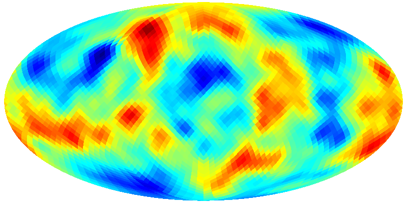
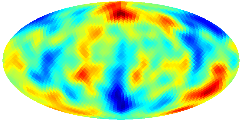
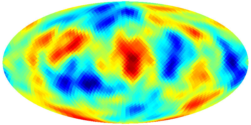
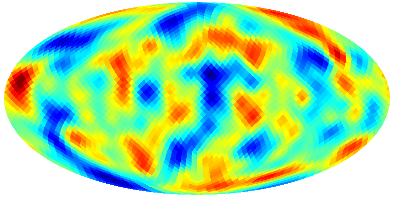
In Fig. 1 we show rows of the pixel-space correlation matrix for a number of multiply-connected topologies as a map, showing the magnitude of the correlation within a particular pixel. For the simply-connected case, the map simply shows the same information as the correlation function ; for the topologically non-trivial cases, we see the correlations depend on distance and direction and differ from pixel to pixel (i.e., from row to row of the matrix). In Fig. 2 we show example maps of CMB anisotropies in universes with these topologies, created by direct realisations of Gaussian fields with the correlation matrices of Fig. 1.


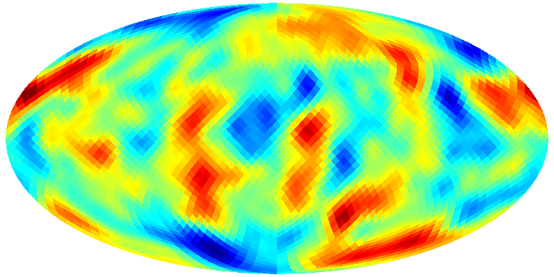

3.2 Bianchi
Bianchi cosmologies include the class of homogeneous but anisotropic cosmologies, where the assumption of isotropy about each point in the Universe is relaxed. For small anisotropy, as demanded by current observations, linear perturbation about the standard FRW model may be applied, leading to a subdominant, deterministic contribution to the CMB fluctuations. In this setting CMB fluctuations may be viewed as the sum of a deterministic Bianchi contribution and the usual stochastic contribution that arises in the CDM model. The deterministic CMB temperature fluctuations that result in the Bianchi models were derived by Barrow et al. (1985), although no dark energy component was included. More recently, Jaffe et al. (2006c), and independently Bridges et al. (2007), extended these solutions for the open and flat Bianchi VIIh models to include cosmologies with dark energy. We defer the details of the CMB temperature fluctuations induced in Bianchi models to these works and give only a brief description here.
Bianchi VIIh models describe a universe with overall rotation, parameterized by an angular velocity, , and a three-dimensional rate of shear, parameterized by the tensor ; we take these to be relative to the axis. The model has a free parameter, first identified by Collins & Hawking (1973), describing the comoving length-scale over which the principal axes of shear and rotation change orientation. The ratio of this length scale to the present Hubble radius is typically denoted , which defines the parameter of type VIIh models through (Barrow et al. 1985)
| (7) |
where the total energy density . The parameter acts to change the “tightness” of the spiral-type CMB temperature contributions that arise due to the geodesic focusing of Bianchi VIIh cosmologies. The shear modes of combinations of orthogonal coordinate axes are also required to describe a Bianchi cosmology. The present dimensionless vorticity may be related to the dimensionless shear modes by (Barrow et al. 1985)
| (8) |
where is the Hubble parameter. The spherical harmonic coefficients of the Bianchi VIIh induced temperature component are proportional to and are non-zero for azimuthal modes only (Barrow et al. 1985; McEwen et al. 2006; Pontzen & Challinor 2007). Hence, varying the phase of corresponds to an azimuthal rotation, i.e. a change of coordinates, while the rotationally invariant part depends on , and we are thus free to choose equality of shear modes (Pontzen & Challinor 2007), which we do for consistency with previous studies (e.g. Jaffe et al. 2005). The amplitude of the deterministic CMB temperature fluctuations induced in Bianchi VIIh cosmologies may be characterised by either or since these parameters influence the amplitude of the induced temperature contribution only and not its morphology. The handedness of the coordinate system is also free in Bianchi VIIh models, hence both left- and right-handed models arise. Since the Bianchi-induced temperature fluctuations are anisotropic on the sky the orientation of the resulting map may vary also, introducing three additional degrees-of-freedom. The orientation of the map is described by the Euler angles444The active Euler convention is adopted, corresponding to the rotation of a physical body in a fixed coordinate system about the , and axes by , and respectively. , where for the swirl pattern typical of Bianchi templates is centred on the South pole.
Examples of simulated Bianchi VIIh CMB temperature maps are illustrated in Fig. 3 for a range of parameters. In the analysis performed herein the BIANCHI2555http://www.jasonmcewen.org/ (McEwen et al. 2013) code is used to simulate the temperature fluctuations induced in Bianchi VIIh models. Bianchi VIIh models induce only large scale temperature fluctuations in the CMB and consequently Bianchi maps have a particularly low band-limit, both globally and azimuthally (i.e., in both and in spherical harmonic space; indeed, as mentioned only those harmonic coefficients with are non-zero).


4 Data description
We use Planck maps that have been processed by the various component-separation pipelines described in Planck Collaboration XII (2014). The methods produce largely consistent maps of the sky, with detailed differences in pixel intensity, noise properties, and masks. Here, we consider maps produced by the Commander-Ruler, NILC, SMICA and SEVEM methods. Each provides its own mask and we also consider the conservative common mask.
We note that because our methods rely on rather intensive pixel- or harmonic-space calculations, in particular considering a full set of three-dimensional orientations and, for the likelihood methods, manipulation of an anisotropic correlation matrix, computational efficiency requires the use of data degraded from the native HEALPix (Górski et al. 2005) resolution of the Planck maps. Because the signatures of either a multiply-connected topology or a Bianchi model are most prominent on large angular scales, this does not result in a significant loss of ability to detect and discriminate amongst the models (see Sect. 5.3). However, it is worth pointing out that the likelihood and matched circles methods are sensitive to different angular scales as applied to Planck data here. The likelihood method explicitly retains only low- (large-scale) information in its correlation matrix, whereas the matched-circles method considers anisotropies at angular scales down to tens of arcminutes (still large in comparison to the native resolution of the Planck maps). Of course, the matched-circles method exploits the correlation of the small-scale patterns along matched circles potentially separated by large angles; this effect is not generated by intrinsically large angular scale anisotropies but by the boundary conditions of the fundamental domain imposed by the multiply connected topology. As described in Sect. 5.1, the matched circles statistic used here damps the anisotropies at the largest angular scales relative to those at smaller scales so sensitivity of the method does not rely on the former.
The topology analyses both rely on degraded maps and masks. The matched-circles method smooths with a 30′ Gaussian filter and degrades the maps to , and uses a mask derived from the SEVEM component separation method. Because the performance of the matched-circles statistic depends on anisotropies on smaller angular scales, it can be significantly degraded by the point source cut. As there are more point sources detected in the Planck maps than in the WMAP maps, the problem of point source masking is more severe in the present case. We mask only those point sources from the full-resolution SEVEM mask with amplitude, after smoothing and extrapolation to the 143 or 217 GHz channels, greater than the faintest source originally detected at those frequencies. The mask derived in this way retains of the sky.
The likelihood method smooths the maps and masks with an 11∘ Gaussian filter and then degrades them to and conservatively masks out any pixel with more than of its original subpixels masked. At full resolution, the common mask retains a fraction of the sky, and when degraded to (the high-resolution point-source masks are largely filled in the degraded masks). The Bianchi analysis is performed in harmonic space, and so does not require explicit degradation in pixel space. Rather, a noisy mask is added in pixel space to effectively marginalise the pixel values in the masked region (as described in more detail below; see also McEwen et al. 2013), before the data are transformed at full resolution into harmonic space and considered only up to a specified maximum harmonic , where correlations due to the mask are taken into account.
Different combinations of these maps and masks are used to discriminate between the topological and anisotropic models described in Sect. 3.
5 Methods
5.1 Topology: circles in the sky
The first set of methods, exemplified by the circles-in-the-sky of Cornish et al. (1998), involves a frequentist analysis using a statistic which is expected to differ between the models examined. For the circles, this uses the fact that the intersection of the topological fundamental domain with the surface of last scattering is a circle, which one potentially views from two different directions in a multiply-connected universe. Of course, the matches are not exact due to noise, foregrounds, the integrated Sachs-Wolfe (ISW) and Doppler effects along the different lines of sight.
By creating a statistic based on the matching of different such circles, we can compare Monte Carlo simulations of both a simply-connected, isotropic null model with specific anisotropic or topological models. We may then calibrate detections and non-detections using Monte Carlo simulations. In principle, these simulations should take into account the complications of noise, foreground contributions, systematics, the ISW and Doppler effects. However, they do not include gravitational lensing of the CMB as the lensing deflection angle is small compared to the minimal angular scale taken into account in our analysis. Note that the null test is generic (i.e., not tied to a specific topology) but any detection must be calibrated with specific simulations for a chosen topology or anisotropic model. A very similar technique can be used for polarisation by taking into account the fact that the polarisation pattern itself is now not directly repeated, but rather that the underlying quadrupole radiation field around each point on the sky is now seen from different directions (Bielewicz et al. 2012). These methods have been applied successfully to COBE DMR and WMAP data, and have recently been shown to be feasible for application to Planck data (Bielewicz et al. 2012).
The idea of using the matched circles to study topology is due to Cornish et al. (1998). In that work, a statistical tool was developed to detect correlated circles in all sky maps of the CMB anisotropy — the circle comparison statistic. In our studies we will use version of this statistic optimised for the small-scale anisotropies as defined by Cornish et al. (2004):
| (9) |
where and denote the Fourier coefficients of the temperature fluctuations around two circles of angular radius centered at different points on the sky, and , respectively, with relative phase . The th harmonic of the temperature anisotropies around the circle is weighted by the factor , taking into account the number of degrees of freedom per mode. Such weighting enhances the contribution of small-scale structure relative to large-scale fluctuations and is especially important since the large-scale fluctuations are dominated by the ISW effect. This can obscure the image of the last scattering surface and reduce the ability to recognise possible matched patterns on it.
The above statistic corresponds to pair of circles with the points ordered in a clockwise direction (phased). For alternative ordering, when along one of the circles the points are ordered in an anti-clockwise direction (anti-phased), the Fourier coefficients are complex conjugated, defining the statistic. This allows the detection of both orientable and non-orientable topologies. For orientable topologies the matched circles have anti-phased correlations while for non-orientable topologies they have a mixture of anti-phased and phased correlations.
The statistic has a range over the interval . Circles that are perfectly matched have , while uncorrelated circles will have a mean value of . Although the statistic can also take negative values for the temperature anisotropy generated by the Doppler term (Bielewicz et al. 2012), anticorrelated circles are not expected for the total temperature anisotropy considered in this work. To find matched circles for each radius , the maximum value is determined.
Because general searches for matched circles are computationally very intensive, we restrict our analysis to a search for pairs of circles centered around antipodal points, so called back-to-back circles. As described above, the maps were also downgraded to , which greatly speeds up the computations required, but with no significant loss of discriminatory power, as seen in Sect. 5.3.1. More details on the numerical implementation of the algorithm can be found in the paper by Bielewicz & Banday (2011).
As mentioned in Sect. 3.1, the constraints we will derive concern topologies that predict matching pairs of back-to-back circles. However, the constraints do not apply to those universes for which the orientation of the matched circles is impossible to detect due to partial masking on the sky. Because of the larger sky fraction removed by the Planck common mask than for WMAP this probability is larger for the analysis of the Planck maps. Moreover, the smaller fraction of the sky used in the search of matched circles results in a false detection level larger with our mask than for the 7-year KQ85 WMAP mask. As a result we obtain weaker — but more conservative — constraints on topology than for similar analyses of WMAP data (Bielewicz & Banday 2011).
To draw any conclusions from an analysis based on the statistic , it is very important to correctly estimate the threshold for a statistically significant match of circle pairs. We used 300 Monte Carlo simulations of CMB maps, described in detail in Section 5.3.1, to establish the threshold such that fewer than 1 % of simulations would yield a false event.
5.2 Bayesian analyses
The second set of methods take advantage of the fact that the underlying small-scale physics is unchanged in both anisotropic and topological models compared to the standard cosmology, and thus a Gaussian likelihood function will still describe the statistics of temperature and polarization on the sky, albeit no longer with isotropic correlations. When considering specific topologies, these likelihood methods instead calculate the pixel-pixel correlation matrix. This has been done for various torus topologies (which are a continuous family of possibilities) in the flat Universe as well as for locally hyperbolic and spherical geometries (which have a discrete set of possibilities for a given value of the curvature). More general likelihood-based techniques have been developed for generic mild anisotropies in the initial power spectrum (Hanson & Lewis 2009), which may have extension to other models. For the Bianchi setting, an isotropic zero-mean Gaussian likelihood is recovered by subtracting a deterministic Bianchi component from the data, where the cosmological covariance matrix remains diagonal in harmonic space but masking introduces non-diagonal structure that must be taken into account.
Because these methods use the likelihood function directly, they can take advantage of any detailed noise correlation information that is available, including any correlations induced by the foreground-removal process. We denote the data by the vector , which may be in the form of harmonic coefficients or pixel temperatures or, in general, coefficients of the temperature expansion in any set of basis functions. We denote the model under examination by the discrete parameter , which can take on the appropriate value denoting the usual isotropic case, or the Bianchi case, or one of the possible multiply-connected universes. The continuous parameters of model are given by the vector , which for this case we can partition into for the cosmological parameters shared with the usual isotropic and simply-connected case, and which denotes the parameters for the appropriate anisotropic case, be it a topologically non-trivial universe or a Bianchi model. Note that all of the anisotropic cases contain “nuisance parameters” which give the orientation of either the fundamental domain or the Bianchi template which we can marginalize over as appropriate.
Given this notation, the posterior distribution for the parameters of a particular model, , is given by Bayes’ theorem:
| (10) |
Here, is the joint prior probability of the standard cosmological parameters and those describing the anisotropic universe , is the likelihood, and the normalizing constant is the Bayesian evidence, which can be used to compare the models to one another.
We will usually take the priors to be simple “non-informative” distributions (e.g., uniform over the sphere for orientations, uniform in length for topology scales, etc.) as appropriate. The form of the likelihood function will depend on the anisotropic model: for multiply-connected models, the topology induces anisotropic correlations, whereas for the Bianchi model, there is a deterministic template, which depends on the Bianchi parameters, in addition to the standard isotropic cosmological perturbations. We will assume that any other non-Gaussian signal (either from noise or cosmology) is negligible (Planck Collaboration XXIII 2014; Planck Collaboration XXIV 2014) and use an appropriate multivariate Gaussian likelihood.
Given the signal and noise correlations, and a possible Bianchi template, the procedure is similar to that used in standard cosmological-parameter estimation, with a few complications. Firstly, the evaluation of the likelihood function is computationally expensive and usually limited to large angular scales. This means that in practice the effect of the topology on the likelihood is usually only calculated on those large scales. Secondly, the orientation of the fundamental domain or Bianchi template requires searching (or marginalizing) over three additional parameters, the Euler angles.
5.2.1 Topology
In topological studies, the parameters of the model consist of , the set of cosmological parameters for the fiducial best-fit flat cosmological model, and , the topological parameters which include the set of compactification lengths for flat toroidal model or the curvature parameter for curved spaces, and a choice of compactification . In our studies we keep fixed, and vary for a select choice of compactifications listed in Sect. 3.1. These parameters define the predicted two-point signal correlation matrix for each model, which are precomputed. Additional internal parameters, including the amplitude of the signal and the angles of orientation of the fundamental domain of the compact space relative to the sky (e.g., parameterized by a vector of the three Euler angles), are maximized and/or marginalized over during likelihood evaluation.
The likelihood, i.e., the probability to find a temperature data map with associated noise matrix given a certain topological model is then given by
| (11) | |||||
Working with a cut-sky, it is often easier to start the analysis with data and a correlation matrix given in pixel space. However, especially in the realistic case of negligible noise on large scales, the matrix is poorly conditioned in pixel space, and pixel space evaluation of the likelihood is, as a rule, not robust. Indeed, there are typically more pixels than independent modes that carry information about the signal (e.g., even in the standard isotropic case, sub-arcminute pixels would not be useful due to beam-smoothing; with anisotropic correlations and masked regions of the sky, more complicated linear combinations of pixels even on large scales may have very little signal content). Therefore in general we expand the temperature map , the theoretical correlation matrix and the noise covariance matrix in a discrete set of mode functions , orthonormal over the pixelized sphere, possibly with weights , , obtaining the coefficients of expansion
| (12) |
Next we select such modes for comparison and consider the likelihood marginalized over the remainder of the modes
| (13) | |||||
where and are restricted to the block of chosen modes. Flexibility in choosing mode functions and their number is used to achieve the compromise between the robust invertibility of the projected matrix on the one hand, and the amount of discriminating information retained in the data on the other. The weights can be used to improve the accuracy of transforms on a pixelized sky.
For full-sky analysis the natural choice of the mode functions is the set of ordinary spherical harmonics which leads to standard harmonic analysis with modes limited to a suitably chosen . Here, where we focus on masked data, we have made a somewhat different choice. As a mode set for comparison we use the largest eigenvectors of the matrix, restricted to the masked sky, for the fiducial flat isotropic model with best-fit parameters . We emphasize that the correlation matrix computed for this reduced dataset has fewer modes, but contains no additional assumptions beyond those of the original .
Since computation of matrices for a range of topological models is expensive, we do not aim to determine the full Bayesian evidence which would require marginalization over all parameters , , an overall amplitude of the correlation matrix (proportional to the physical amplitude or the scalar amplitude ) , and orientation (Euler angles) , and would in addition be sensitive to the prior probabilities assumed for the size of the fundamental domain. Instead we directly compare the likelihood along the changing set of that has as its limit the flat fiducial model defined by . In case of toroidal topology such a limit is achieved by taking compactification lengths to infinity, while for curved models we vary in comparison to the flat limit . In the latter case, for the spherical spaces we change and together with to track the CMB geometrical degeneracy line in which the recombination sound speed, initial fluctuations, and comoving distance to the last scattering surface are kept constant (e.g., Bond et al. 1997; Zaldarriaga & Seljak 1997; Stompor & Efstathiou 1999), and for hyperbolic spaces we vary while keeping and fixed to fiducial values. Note that hyperbolic multi-connected spaces, in contrast to tori and the single-action positive curvature manifolds considered in this paper, are not only anisotropic but also inhomogeneous. Therefore, the likelihood is expected to be dependent on the position of the observer. We do not study this dependence here.
For each parameter choice, we find the likelihood at the best orientation of the topology with respect to the sky after marginalizing over the amplitude of the signal (hence, this can be considered a profile likelihood with respect to the orientation parameters). This likelihood is compared both with the fiducial model applied to the observed temperature map and with the likelihood of the topological model applied to the simulated realization of the isotropic map drawn from the fiducial model. Such a strategy is optimized for the detection of topological signatures. For non-detections, the marginalized likelihood can be a better probe of the overall power of the data to reject a non-trivial topology, and so for real data below, we also show the likelihood marginalized over the orientations . We estimate the marginalized likelihood from the random sample of 10,000 orientations, drawn statistically uniformly on the sphere of unit quaternions representing rotations of the fundamental domain relative to the observed sky.
5.2.2 Bianchi
For the Bianchi analysis the posterior distribution of the parameters of model is given by Bayes’ Theorem, specified in Eq. 10, similar to the topological setting. The approach of McEwen et al. (2013) is followed, where the likelihood is made explicit in the context of fitting a deterministic Bianchi template embedded in a stochastic CMB background, defined by the power spectrum for a given cosmological model with parameters . The Bianchi VIIh parameters are denoted . The corresponding likelihood is given by
| (14) |
where
| (15) |
and and are the spherical harmonic coefficients of the data and Bianchi template, respectively, considered up to the harmonic band-limit . A band-limit of is considered in the subsequent analysis for computational tractibility and since this is sufficient to capture the structure of the CMB temperature fluctuations induced in Bianchi VIIh models in the vacinity of the best-fit model found in WMAP data (see, e.g., McEwen et al. 2006). The likelihood is computed in harmonic space where rotations of the Bianchi template can be performed efficiently (McEwen et al. 2006).
The covariance matrix depends on whether the full-sky or partial-sky masked setting is considered. In the full-sky setting as first considered by Bridges et al. (2007), where is the diagonal CMB covariance matrix with entries on the diagonal. In the case of a zero Bianchi component, Eq. 14 then reduces to the likelihood function used commonly to compute parameter estimates from the power spectrum estimated from CMB data (e.g. Verde et al. 2003). In the masked setting considered subsequently, the situation is a little more involved.
In order to handle a mask in the harmonic space analysis of Bianchi models we follow the approach of McEwen et al. (2013), where masking noise is added to the data to effectively marginalise over the pixel values of the data in the masked region. The masking noise is chosen to be zero-mean and large in the masked region of the data, and zero elsewhere. Consequently, the masking noise is anisotropic over the sky but may be chosen to be uncorrelated, and may thus be defined by its covariance
| (16) |
where is Kronecker delta symbol, denotes the angular coordinate of pixel , and the variance of the noise for pixel is given by a constant value in the masked regions and zero elsewhere. By synthetically adding masking noise that is much larger than the original data in the masked region of the sky, we effectively marginalise over the pixel values of the data in this region. The noisy mask introduces coupling in harmonic space that must be accounted for in the analysis. The covariance matrix of the resultant data is given by , where is the non-diagonal mask covariance matrix:
| (17) |
and is the area of pixel (see McEwen et al. (2013) for further details).
The of the likelihood for the Bianchi case hence differs from the topology case by the nonzero Bianchi template and the use of a correlation matrix to account for the presence of the mask.
In the most physically motivated scenario, the Bianchi and cosmological parameters are coupled (e.g. the total density of the Bianchi and standard cosmological model are identical). However, it is also interesting to consider Bianchi templates as phenomenological models with parameters decoupled from the standard cosmological parameters, particularly for comparison with previous studies. Both scenarios are considered in the subsequent analysis. In the decoupled scenario a flat cosmological model is considered, whereas in the coupled scenario an open cosmological model is considered to be consistent with the Bianchi VIIh model; we label these models the flat-decoupled-Bianchi model and the the open-coupled-Bianchi model, respectively.
To determine whether the inclusion of a Bianchi component better describes the data the Bayesian evidence is examined, as given by
| (18) |
Using the Bayesian evidence to distinguish between models naturally incorporates Occam’s razor, trading off model simplicity and accuracy. In the absence of any prior information on the preferred model, the Bayes factor given by the ratio of Bayesian evidences (i.e., ) is identical to the ratio of the model probabilities given the data. The Bayes factor is thus used to distinguish models. The Jeffreys scale (Jeffreys 1961) is often used as a rule-of-thumb when comparing models via their Bayes factor. The log-Bayes factor (also called the log-evidence difference) represents the degree by which the model corresponding to is favoured over the model corresponding to , where: is regarded as inconclusive; as significant; as strong; and as conclusive (without loss of generality we have assumed ). For reference, a log-Bayes factor of 2.5 corresponds to odds of 1 in 12, approximately, while a factor of 5 corresponds to odds of 1 in 150, approximately.
The ANICOSMO666http://www.jasonmcewen.org/ code (McEwen et al. 2013) is used to perform a Bayesian analysis of Bianchi VIIh models, which in turn uses the public MultiNest777http://www.mrao.cam.ac.uk/software/multinest/ code (Feroz & Hobson 2008; Feroz et al. 2009) to sample the posterior distribution and compute evidence values by nested sampling (Skilling 2004). We sample the parameters describing the Bianchi VIIh model and those describing the standard cosmology simultaneously.
5.3 Simulations and Validation
5.3.1 Topology
Circles-in-the-Sky
Before beginning the search for pairs of matched circles in the Planck data, we validate our algorithm using simulations of the CMB sky for a universe with 3-torus topology for which the dimension of the cubic fundamental domain is , and with cosmological parameters corresponding to the model (see Komatsu et al. 2011, Table 1) determined from the 7-year WMAP results combined with the measurements of the distance from the baryon acoustic oscillations and the Hubble constant. We performed simulations computing directly the coefficients up to the multipole of order as described in Bielewicz & Banday (2011) and convolving them with the same smoothing beam profile as used for the data, i.e., a Gaussian beam with 30′ FWHM. In particular, we verified that our code is able to find all pairs of matched circles in such a map. The map with marked pairs of matched circles with radius and the statistic for the map are shown in Fig. 4 and Fig. 5, respectively. Note that the peak amplitudes in the statistic, corresponding to the temperature correlation for matched circles, decrease with radius of the circles. Cornish et al. (2004) noted that this is primarily caused by the Doppler term, which becomes increasingly anticorrelated for circles with radius smaller than .
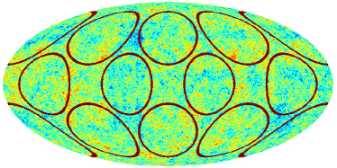
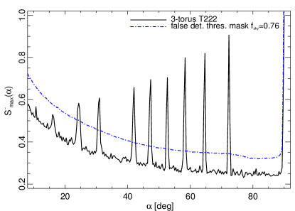
The intersection of the peaks in the matching statistic with the false detection level estimated for the CMB map corresponding to the simply-connected universe defines the minimum radius of the correlated circles which can be detected for this map. The height of the peak with the smallest radius seen in Fig. 5 indicates that the minimum radius is about .
For the Monte Carlo simulations of the CMB maps for the simply-connected universe we used the same cosmological parameters as for the multi-connected universe, i.e., corresponding to the CDM model determined from the 7-year WMAP results. The maps were also convolved with the same beam profile as for the simulated map for the 3-torus universe and data, as well as masked with the same cut used for the analysis of data. The false detection threshold was established such that fewer than 1 % of 300 Monte Carlo simulations would yield a false event.
Bayesian Analysis
Because of the expense of the calculation of the correlation matrix, we wish to limit the number of three-dimensional wavevectors we consider, as well as the number of spherical harmonic modes , and finally the number of different correlation matrices as a whole. We need to ensure that the full set of matrices that we calculate contains all of the available information on the correlations induced by the topology in a sufficiently fine-grained grid. For this purpose, we consider the Kullback-Leibler (KL) divergence as a diagnostic (see, e.g., Kunz et al. 2006, 2008, for applications of the KL divergence to topology). The KL divergence between two probability distributions and is given by
| (19) |
If the two distributions are Gaussian with correlation matrices and , this expression simplifies to
| (20) |
and is thus a measure of the discrepancy between the correlation matrices. The KL divergence can be interpreted as the ensemble average of the log-likelihood-ratio between realizations of the two distributions. Hence, they enable us to probe the ability to tell if, on average, we can distinguish realizations of from a fixed without having to perform a brute-force Monte Carlo integration. Thus, the KL divergence is related to ensemble averages of the likelihood-ratio plots that we present for simulations (Fig. 10) and real data (Sect. 6), but does not depend on simulated or real data.
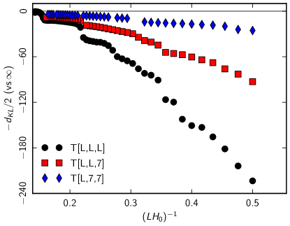
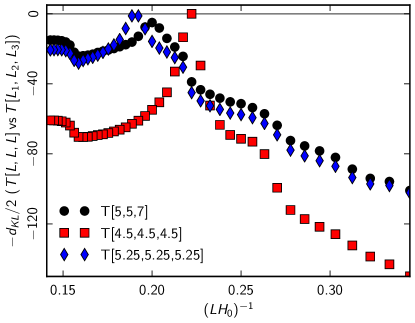
We first use the KL divergence to determine the size of the fundamental domain which we can consider to be equivalent to the simply-connected case (i.e., the limit in which all dimensions of the fundamental domain go to infinity). We note that in our standard CDM model, the distance to the surface of last scattering is . We would naively expect that as long as the sphere enclosing the last scattering surface can be enclosed by the fundamental domain (), we would no longer see the effects of non-trivial topology. However, because the correlation matrix includes the full three-dimensional correlation information (not merely the purely geometrical effects of completely correlated points) we would see some long-scale correlation effects even for larger fundamental domains. In Fig. 6 we show the KL divergence (as a function of so that the simply-connected limit is at a finite position) for the (cubic), (chimney) and (slab) spaces and show that it begins to level off for , although these topologies are still distinguishable from the torus which is yet closer to the value for a simply-connected universe . These figures indicate that a length of is an acceptable proxy for the simply-connected infinite Universe. The figures, as well as the likelihoods computed on simulations and data, show steps and other structures on a variety of scales corresponding to the crossing of the different length scales of the fundamental domain , , and crossing the last scattering surface; smaller fundamental domains with longer intersections with the last scattering surface are easier to detect.
Computational limitations further prevent us from calculating the likelihood at arbitrary values of the fundamental domain size parameters. We must therefore ensure that our coarse-grained correlation matrices are sufficient to detect a topology even if it lies between our gridpoints. In Fig. 7 we show the KL divergence as a function of the size of the fundamental domain, relative to various models, both aligned with our grid () and in between our grid points (). We see that the peak is wide enough that we can detect a peak within of the correct value. We also show that we can detect anisotropic fundamental domains even when scanning through cubic tori: we show a case which approximates a “chimney” universe with one direction much larger than the distance to the last scattering surface.
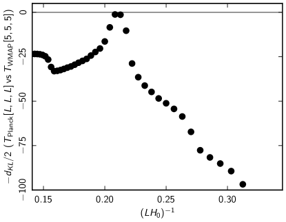
Because our topological analyses do not simultaneously vary the background cosmological parameters along with those describing the topology, we also probe the sensitivity to the cosmology. In Fig. 8 we show the effect of varying the fiducial cosmology from the Planck Collaboration XVI (2014) best-fit values to those reported by WMAP (Komatsu et al. 2011).888We use the wmap7+bao+h0 results from http://lambda.gsfc.nasa.gov. We see that this induces a small bias of but does not hinder the ability to detect a non-trivial topology. This indicates that small deviations from the correct background cosmology do not hinder our ability to detect (or rule out) topological signals.
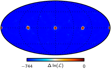
We have also directly validated the topological Bayesian techniques with simulations. In Fig. 9 we show the log-likelihood for the above simulations as a function of two of the Euler angles, maximized over the third. We find a strong peak at the correct orientation, with a multiplicity due to the degenerate orientations corresponding to the faces of the cube (there are peaks at the North and South poles, which are difficult to see in this projection). Note that the peaks correspond to ratios of more than compared to the relatively smooth minima elsewhere.
In Fig. 10 we also test the ability of the Bayesian likelihood technique to detect the compactification of the space in the simulated temperature realizations drawn from the dodecahedral closed model. For curved geometries, the size of the fundamental domain is fixed with respect to the varying curvature scale (), whereas the distance to the last scattering is constant. Hence we plot the likelihood as a function of , inversely proportional to the scale of the fundamental domain.
Two mulitply-connected realizations of the sky were tested: one corresponding to the space in which the last scattering sphere can be just inscribed into the fundamental domain, , when just the first large angle correlations appear, and the second drawn from a somewhat smaller space for which . We see detections in both cases, stronger as the fundamental domain shrinks relative to . We also calculate the likelihood for a model known to be simply-connected.
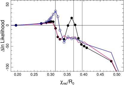
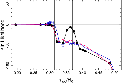
Note that the likelihood taken at the best orientations of the compact models generically shows a slight increase relative to that for the limiting simply connected space as one brings the size of the fundamental domain down to the size of the last scattering surface (), followed, in the absence of signal in the map, by a rapid drop as soon as the models smaller than are applied. This small increase is also present in the fiducial exactly isotropic sky, a single realization of which is shown in the figure, but is a generic feature irrespective of the topology being tested (occurring also in models with ), and thus should not be taken as an indication for compact topology. The reason for the increase is the possibility of aligning the model with a weak anisotropic correlation feature with chance patterns of a single sky realization. However the fit drastically worsens as soon as the correlation features in a model become pronounced. Moreover, the feature becomes considerably less significant when the likelihood is marginalized over the orientation (Euler angles) of the fundamental domain.
All of these results (KL divergences and likelihoods) were computed with , corresponding approximately to , indicating that this is more than adequate for detecting even relatively small fundamental domains such as the case simulated above. We also calculate between the correlation matrices for the torus (as a proxy for the simply-connected case) and the torus, as a function of the maximum multipole used in the calculation of the correlation matrix: we find that continues to increase beyond . Thus, higher-resolution maps (as used by the matched-circles methods) contain more information, but with the very low level of noise in the Planck CMB maps, would nonetheless give a robust detection of a multiply-connected topology, even with the conservative foreground masking we apply.
We note that it is difficult to compress the content of these likelihood figures down to limits upon the size of the fundamental domain. This arises because it is difficult to provide a physically-motivated prior distribution for quantities related to the size of the fundamental domain. Most naive priors would diverge toward arbitrarily large fundamental domain sizes or would otherwise depend on arbitrary limits to the topological parameters.
5.3.2 Bianchi
The ANICOSMO code (McEwen et al. 2013) is used to perform a Bayesian analysis of Bianchi VIIh models, which has been extensively validated by McEwen et al. (2013) already; we briefly summarise the validation performed for the masked analysis. In McEwen et al. (2013) a CMB map is simulated, in which a simulated Bianchi temperature map with a large vorticity (i.e., amplitude) is embedded, before applying a beam, adding isotropic noise and applying a mask. Both the underlying cosmological and Bianchi parameters used to generate the simulations are well recovered. For this simulation the coupled Bianchi model is favoured over CDM, with a log-Bayes factor of . As expected, one finds that the log-Bayes factor favours CDM in simulations where no Bianchi component is added. For further details see McEwen et al. (2013).
6 Results
We now discuss the results of applying the circles-in-the-sky and likelihood methods to Planck data to study topology and Bianchi VIIh cosmologies.
6.1 Topology
Neither the circles-in-the-sky search nor the likelihood method find evidence for a multiply-connected topology. We show the matched circle statistic in Fig. 11. We do not find any statistically significant correlation of circle pairs in any map. As seen in Fig. 5, the minimum radius at which the peaks expected for the matching statistic are larger than the false detection level is . Thus, we can exclude at the confidence level of 99 % any topology that predicts matching pairs of back-to-back circles larger than this radius, assuming that relative orientation of the fundamental domain and mask allows its detection. This implies that in a flat universe described otherwise by the Planck fiducial CDM model, a confidence-limit lower bound on the size of the fundamental domain is . This is better than the limits from the marginalized likelihood ratios below for the tori and octahedron topologies and slightly worse than the limits for the dodecahedron and truncated cube. However, this constraint is not limited only to these few topologies. The frequentist analysis provides constraints upon a much wider class of topologies than those explicitly considered in the Bayesian likelihood approach; it concerns all topologies listed in Sect. 3.1.
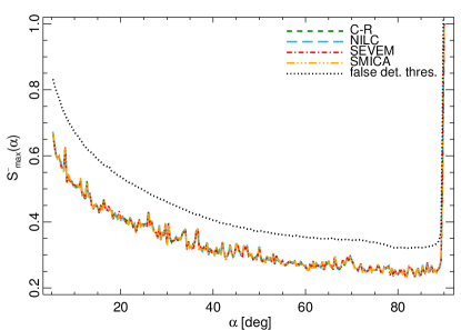
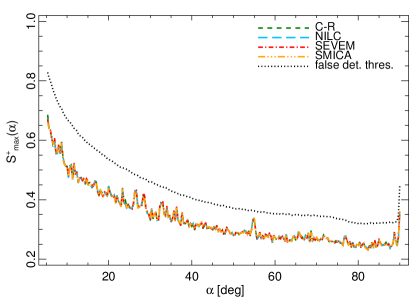
The likelihood method also show no evidence of a multiply connected universe. We present the likelihood for various models. In Fig. 12 we show the likelihood (marginalized over amplitude and maximized over orientation of the fundamental domain) for the cubic torus, fixing the background cosmology to the best-fit flat Universe Planck model (Planck Collaboration XVI 2014). We see that this is maximized for , i.e., showing no evidence for non-trivial topology. Note that the likelihood shows mild features as the size goes through the other scales associated with the topology, in particular a small increase in the likelihood when the scale of the inscribed sphere is crossed. However, the same increase is found when the toroidal model is compared to a single realization of a strictly isotropic fiducial sky, and thus, should not be interpreted as a detection of multi-connected topology. The origin of this likelihood behaviour at best fit angles is that the freedom of orientation can be used to align small enhancements in large-angle correlations in the anisotropic model with random features in the given single realization of the sky. When marginalized over all possible orientations the effect is significantly reduced; the slight rise is from a likelihood of , which is comparable to the numerical noise inherent in our stochastic integration. For even smaller spaces, more extensive correlations of the temperature can no longer be accommodated and for the likelihood of the T3 cubic toroidal model drops quickly, although not strictly monotonically.
In Figs. 13 and 14 we show the likelihood for the chimney and slab topologies, which are also maximized in the simply-connected limit. The T2 chimney, with only two compact dimensions, is less constrained than the T3 cube, and the T1 slab, with one compact dimension, even less so.
We find similar limits for the topologies allowed in a closed universe with a locally spherical geometry. In Fig. 15 we show the likelihood for the dodecahedral fundamental domain, in Fig. 16 for the truncated cube, and in Fig. 17 for the octahedron. In this case, we do not fix the background cosmological model, but rather account for the geometrical degeneracy line which links and with . The degeneracy relations are approximated as and . As in the toroidal case, there is no detection of a small space at the level expected from the simulations of Sect. 5. Fundamental domains larger than the last scattering diameter are preferred for the dodecahedral and truncated cube spaces with somewhat weaker restriction for the octahedral case. Note that an observationally motivated prior on or would be yet more restrictive on the fundamental domain size. For all three topologies, again as in the toroidal case, the maximum of the likelihood at best fit orientation is detected for the finite volume spaces with at the level relative to the fiducial flat simply-connected model. Since this feature is seen in the isotropic fiducial sky as well, we cannot take it as an indication of a detection of a multi-connected space. In the case of curved spaces we see that this mild increase disappears when we consider the likelihood marginalized over orientations.
We present numerical limits for these flat and positively curved spaces in Table 2. Because of the one-sided nature of these limits, we characterize the shape of the likelihood by the steepness of its fall from the value as the scale of the fundamental domain goes to infinity (i.e., the simply-connected limit). Hence, we show limits for , (roughly equivalent to a — 99 % confidence limit — fall for a Gaussian; because of the very steep gradient, the limits are very similar) and (). Note that the limits differ depending on whether we marginalize or maximize the likelihood over the orientation angles. We show lower limits on the quantity ( for a torus with edge length ) in units of the last scattering distance (in conventional units, for the fiducial Planck parameters; Planck Collaboration XVI 2014). In most cases, the limits are roughly — the scale of the fundamental domain must be greater than that of the last scattering surface. We place the most restrictive limits on the dodecahedron with using marginalized values for . Conversely, the chimney and slab spaces are less constrained as the expected correlations are weaker in one or two directions; for the slab space, we only constrain .
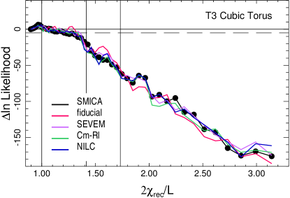
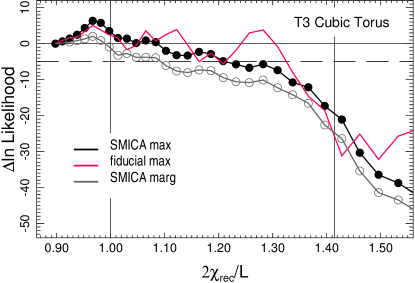
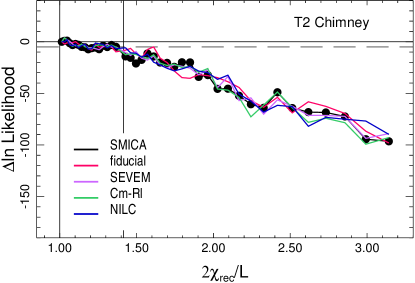
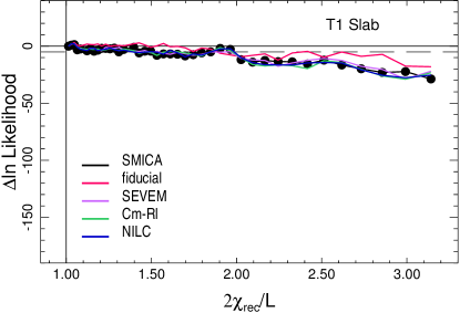
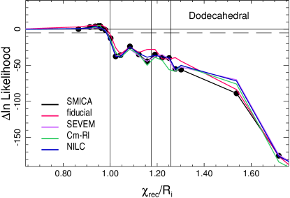
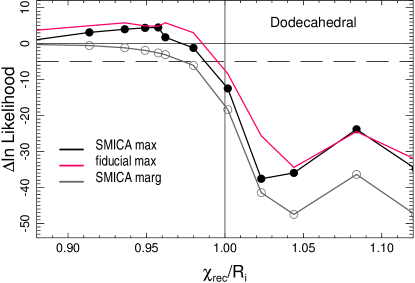
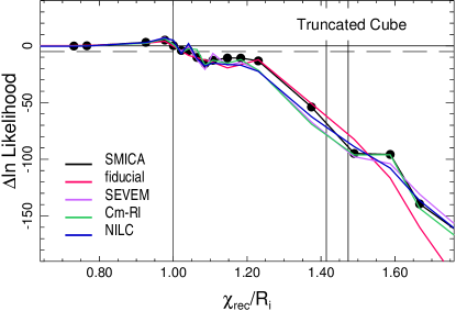
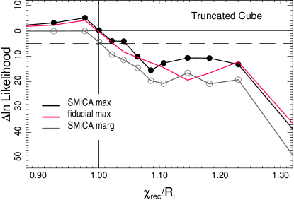
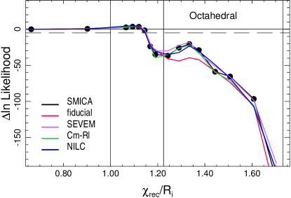
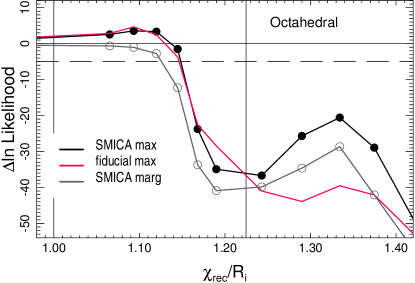
|
||||||||||||||||||||||||||||||||||||||||||||||||||||||||||||||||||
In Fig. 18 we show the likelihood for the two hyperbolic models listed in Table 1, which also show no detection of the multi-connected topology. In the hyperbolic case we space the range of space sizes by varying while keeping as well as constant at fiducial values.
All of these results show at least some increase in the likelihood for certain orientations when one of the characteristic scales of the fundamental domain (, , or ) just exceed the surface of last scattering, and so no longer produces matched patterns, but induces extra correlations at large angular separations. Chance patterns can then mimic these correlations, and this is exacerbated by our conservative sky masks, which allow arbitrary patterns in the masked regions.
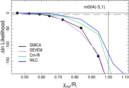
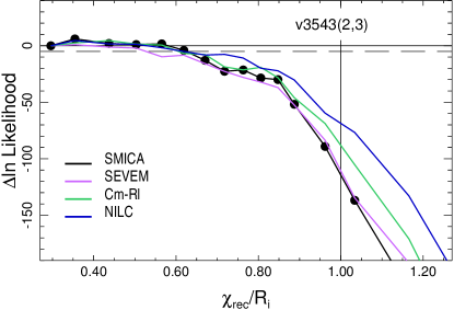
6.2 Bianchi
Masked Planck data are analysed for evidence of a Bianchi VIIh component, where the prior parameter ranges adopted are the same as those specified by McEwen et al. (2013). The analysis is performed on the SMICA component-separated map, using the mask defined for this method, and is repeated on the SEVEM component-separated map for validation purposes (using the mask defined for the SEVEM method). The Bayes factors for the various Bianchi VIIh models and the equivalent standard cosmological models are shown in Table 3.
| Model | SMICA | SEVEM |
|---|---|---|
| Flat-decoupled-Bianchi (left-handed) | ||
| Flat-decoupled-Bianchi (right-handed) | ||
| Open-coupled-Bianchi (left-handed) | ||
| Open-coupled-Bianchi (right-handed) |

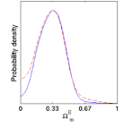
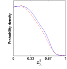
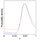
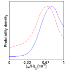
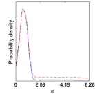
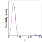
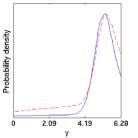
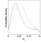
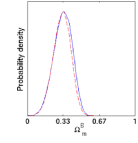
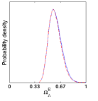
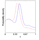
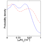
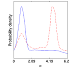
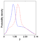
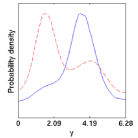
For the phenomenological flat-decoupled-Bianchi model, evidence in support of a left-handed Bianchi template is found. On the Jeffreys scale (Jeffreys 1961), evidence for this model would be referred to as strong for the SMICA map and significant for the SEVEM map. For both SMICA and SEVEM component-separated data, recovered posterior distributions for the flat-decoupled-Bianchi model are shown in Fig. 19(a), where similar posterior distributions are recovered for both component separation methods. Recall that the Bianchi parameters are decoupled from the standard cosmology in the flat-decoupled-Bianchi model, hence for this model and are specific to the Bianchi model and should not be compared with standard values. The maximum a posteriori (MAP) best-fit template found for SMICA component-separated data is shown in Fig. 20(b), with the difference between this template and the template found in WMAP 9-year data (McEwen et al. 2013) shown in Fig. 21. Note that the template found in Planck data is very similar to the template found in WMAP 9-year data (McEwen et al. 2013), which in turn is similar to the template first found by Jaffe et al. (2005). However, the template found in WMAP 9-year data (McEwen et al. 2013) is only significant in full-sky data, but not when the 9-year KQ75 WMAP mask (Bennett et al. 2012) is applied. Since the Planck SMICA and SEVEM masks are less conservative than the KQ75 mask, these findings suggest data near the Galactic plane may be playing a considerable role in supporting a Bianchi component in Planck data. The SMICA CMB map and a Bianchi-subtracted version of this map are also shown in Fig. 20. The best-fit parameters of the templates found in Planck SMICA and SEVEM component-separated data are displayed in Table 4, for both the MAP and mean-posterior estimates. The analysis was also performed on a SMICA component-separated Gaussian simulation, yielding a null detection (i.e., no evidence for a Bianchi component), as expected.
| Bianchi Parameter | SMICA | SEVEM | ||||
|---|---|---|---|---|---|---|
| MAP | Mean | MAP | Mean | |||
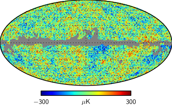
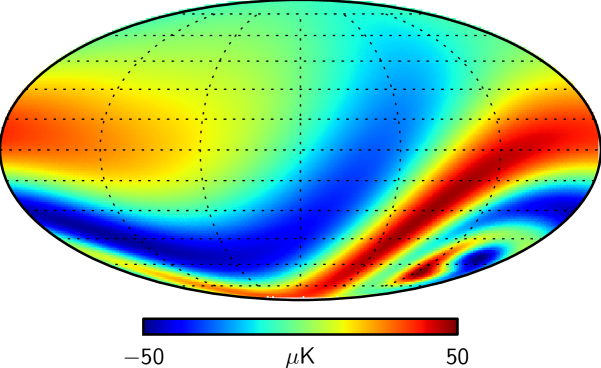
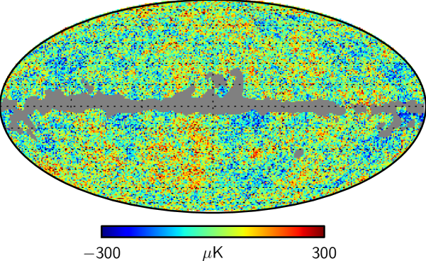
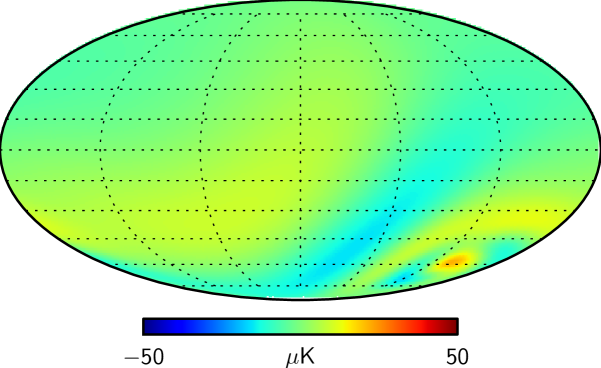
For the most physically motivated open-coupled-Bianchi model where the Bianchi VIIh model is coupled to the standard cosmology, there is no evidence in support of a Bianchi contribution. Recovered posterior distributions for the open-coupled-Bianchi model are shown in Fig. 19(b) for both SMICA and SEVEM component-separated data. Although the cosmological Bianchi parameters agree reasonably well between these different component-separated data, the posterior distributions recovered for the Euler angles differ. For SEVEM data, an additional mode of the posterior distribution is found; the mode found with SMICA data is still present in SEVEM data but is not dominant. Consequently, the best-fit estimates for the Euler angles differ between the SMICA and SEVEM component-separated data. Note that the additional mode found in SEVEM data is also present in WMAP 9-year data (McEwen et al. 2013). The resulting best-fit parameters for the the open-coupled-Bianchi model are displayed in Table 5, while the corresponding MAP best-fit maps are shown in Fig. 22. Nevertheless, for both SMICA and SEVEM data the Bayes factors computed (Table 3) do not favour the inclusion of any Bianchi component for the open-coupled-Bianchi model. Planck data thus do not provide evidence in support of Bianchi VIIh cosmologies. However, neither is it possible to conclusively discount Bianchi VIIh cosmologies in favour of CDM cosmologies. The constraints (95% confidence level) on the vorticity of the physical coupled Bianchi VIIh left-handed models and (95% confidence level) for right-handed models are recovered from SMICA component-separated data.
| Bianchi Parameter | SMICA | SEVEM | ||||
|---|---|---|---|---|---|---|
| MAP | Mean | MAP | Mean | |||
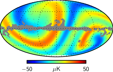
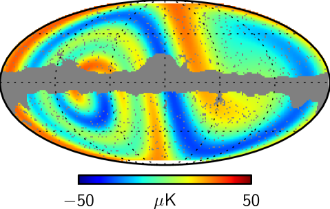
7 Discussion
We have used the Planck temperature anisotropy maps to probe the large-scale structure of spacetime. We have calculated the Bayesian likelihood for specific topological models in universes with locally flat, hyperbolic and spherical geometries, all of which find no evidence for a multiply-connected topology with a fundamental domain within the last scattering surface. After calibration on simulations, direct searches for matching circles resulting from the intersection of the fundamental topological domain with the surface of last scattering also give a null result at high confidence. These results use conservative masks of the sky, unlike previous WMAP results, which used full-sky internal linear combination maps (not originally intended for cosmological studies) or less conservative foreground masks. Hence, the results presented here, while corroborating the previous non-detections, use a single, self-consistent, and conservative dataset. The masked sky also increases the possibility of chance patterns in the actual sky mimicking the correlations expected for topologies with a characteristic scale near that of the last scattering surface.
Depending on the shape of the fundamental domain, we find (Table 2) with detailed 99 % confidence limits (considering the likelihood marginalized over the orientation of the fundamental domain) varying from for the cubic torus in a flat universe to for the dodecahedron in a positively curved universe, with somewhat weaker constraints for poorly-proportioned spaces that are considerably larger along some directions. In the case of the torus and octahedron topologies, a tighter constraint of comes from the matched circles method (albeit with a somewhat different interpretation of frequentist and Bayesian limits). The constraint derived using this method applies to a wide class of topologies, listed in Sect. 3.1, predicting matching pairs of back-to-back circles.
Note that the results derived using the likelihood method make use of the expected pixel-space correlations as a unique signal of non-trivial topology. Hence, although a small fundamental domain will suppress power on the largest scales of the CMB, observation of such low power on large scales as observed by COBE (Bond et al. 2000), and confirmed by WMAP (Luminet et al. 2003), is not sufficient for the detection of topology. Conversely, because our methods search directly for these correlations (and indeed marginalize over the amplitude of fluctuations), a slight modification of the background FRW cosmology by lowering power in some or all multipoles (Planck Collaboration XV 2014) will not affect the ability to detect the correlations induced by such topologies.
Similarly, using a Bayesian analysis we find no evidence for a physical, anisotropic Bianchi VIIh universe. However, Planck data do provide evidence supporting a phenomenological Bianchi VIIh component, where the parameters of the Bianchi component are decoupled from standard cosmology. The resulting best-fit Bianchi VIIh template found in Planck data is similar to that found in WMAP data previously (Jaffe et al. 2005; McEwen et al. 2013). However, although this Bianchi component can produce some of the (possibly anisotropic) temperature patterns seen on the largest angular scales (see also Planck Collaboration XXIII 2014), there is no set of cosmological parameters which can simultaneously produce these patterns and the observed anisotropies on other scales. Moreover, the parameters of the best-fit Bianchi VIIh template in the decoupled setting are in strong disagreement with other measurements of the cosmological parameters.
These results are expected from previous measurements from COBE and WMAP, but Planck’s higher sensitivity and lower level of foreground contamination provides further confirmation. We have shown that the results are insensitive to the details of the preparation of the temperature maps (in particular, the method by which the cosmological signal is separated from astrophysical foreground contamination). Future Planck measurement of CMB polarization will allow us to further test models of anisotropic geometries and non-trivial topologies and may provide more definitive conclusions, for example allowing us to moderately extend the sensitivity to large-scale topology (Bielewicz et al. 2012).
Acknowledgements.
The development of Planck has been supported by: ESA; CNES and CNRS/INSU-IN2P3-INP (France); ASI, CNR, and INAF (Italy); NASA and DoE (USA); STFC and UKSA (UK); CSIC, MICINN, JA and RES (Spain); Tekes, AoF and CSC (Finland); DLR and MPG (Germany); CSA (Canada); DTU Space (Denmark); SER/SSO (Switzerland); RCN (Norway); SFI (Ireland); FCT/MCTES (Portugal); and PRACE (EU). A description of the Planck Collaboration and a list of its members, including the technical or scientific activities in which they have been involved, can be found at http://www.sciops.esa.int/index.php?project=planck&page=Planck_Collaboration. The authors thank the anonymous referee for helpful comments and acknowledge the use of the UCL Legion High Performance Computing Facility (Legion@UCL), and associated support services, in the completion of this work. Part of the computations were performed on the Andromeda cluster of the University of Geneve, the Hopper Cray XE6 at NERSC and on the GPC supercomputer at the SciNet HPC Consortium. SciNet is funded by: the Canada Foundation for Innovation under the auspices of Compute Canada; the Government of Ontario; Ontario Research Fund - Research Excellence; and the University of Toronto.References
- Aurich (1999) Aurich, R. 1999, ApJ, 524, 497
- Aurich et al. (2008) Aurich, R., Janzer, H. S., Lustig, S., & Steiner, F. 2008, Classical and Quantum Gravity, 25, 125006
- Aurich & Lustig (2013) Aurich, R. & Lustig, S. 2013, MNRAS, 433, 2517
- Aurich et al. (2005) Aurich, R., Lustig, S., & Steiner, F. 2005, Classical and Quantum Gravity, 22, 2061
- Aurich et al. (2006) Aurich, R., Lustig, S., & Steiner, F. 2006, MNRAS, 369, 240
- Aurich et al. (2004) Aurich, R., Lustig, S., Steiner, F., & Then, H. 2004, Classical and Quantum Gravity, 21, 4901
- Barrow (1986) Barrow, J. D. 1986, Canadian Journal of Physics, 64, 152
- Barrow et al. (1985) Barrow, J. D., Juszkiewicz, R., & Sonoda, D. H. 1985, Mon. Not. Roy. Astron. Soc., 213, 917
- Bennett et al. (1996) Bennett, C. L., Banday, A. J., Gorski, K. M., et al. 1996, ApJ, 464, L1
- Bennett et al. (2003) Bennett, C. L., Halpern, M., Hinshaw, G., et al. 2003, ApJS, 148, 1
- Bennett et al. (2012) Bennett, C. L., Larson, D., Weiland, J. L., et al. 2012, ArXiv e-prints
- Bielewicz & Banday (2011) Bielewicz, P. & Banday, A. J. 2011, MNRAS, 412, 2104
- Bielewicz et al. (2012) Bielewicz, P., Banday, A. J., & Górski, K. M. 2012, MNRAS, 421, 1064
- Bielewicz & Riazuelo (2009) Bielewicz, P. & Riazuelo, A. 2009, MNRAS, 396, 609
- Bond & Efstathiou (1987) Bond, J. R. & Efstathiou, G. 1987, Monthly Notices of the Royal Astronomical Society, 226, 655
- Bond et al. (1997) Bond, J. R., Efstathiou, G., & Tegmark, M. 1997, Monthly Notices of the Royal Astronomical Society, 291, L33
- Bond et al. (2000) Bond, J. R., Jaffe, A. H., & Knox, L. E. 2000, Astrophysical Journal, 533, 19
- Bond et al. (1998) Bond, J. R., Pogosyan, D., & Souradeep, T. 1998, Classical and Quantum Gravity, 15, 2671
- Bond et al. (2000a) Bond, J. R., Pogosyan, D., & Souradeep, T. 2000a, Phys. Rev. D, 62, 043005
- Bond et al. (2000b) Bond, J. R., Pogosyan, D., & Souradeep, T. 2000b, Phys. Rev. D, 62, 043006
- Bridges et al. (2008) Bridges, M., McEwen, J. D., Cruz, M., et al. 2008, Mon. Not. Roy. Astron. Soc., 390, 1372
- Bridges et al. (2007) Bridges, M., McEwen, J. D., Lasenby, A. N., & Hobson, M. P. 2007, Mon. Not. Roy. Astron. Soc., 377, 1473
- Bunn et al. (1996) Bunn, E. F., Ferreira, P. G., & Silk, J. 1996, Phys. Rev. Lett., 77, 2883
- Caillerie et al. (2007) Caillerie, S., Lachièze-Rey, M., Luminet, J.-P., et al. 2007, Astronomy and Astrophysics, 476, 691
- Cayón et al. (2006) Cayón, L., Banday, A. J., Jaffe, T., et al. 2006, Mon. Not. Roy. Astron. Soc., 369, 598
- Collins & Hawking (1973) Collins, C. B. & Hawking, S. W. 1973, MNRAS, 162, 307
- Cornish & Spergel (1999) Cornish, N. J. & Spergel, D. N. 1999, math/9906017
- Cornish et al. (1998) Cornish, N. J., Spergel, D. N., & Starkman, G. D. 1998, Classical and Quantum Gravity, 15, 2657
- Cornish et al. (2004) Cornish, N. J., Spergel, D. N., Starkman, G. D., & Komatsu, E. 2004, Physical Review Letters, 92, 201302
- Coule & Martin (2000) Coule, D. & Martin, J. 2000, Physical Review D, 61, 063501
- Cruz et al. (2006) Cruz, M., Tucci, M., Martínez-González, E., & Vielva, P. 2006, Mon. Not. Roy. Astron. Soc., 369, 57
- de Oliveira-Costa & Smoot (1995) de Oliveira-Costa, A. & Smoot, G. F. 1995, ApJ, 448, 477
- de Sitter (1917) de Sitter, W. 1917, Proc. Roy. Acad. Amsterdam, 20, 229
- Dineen et al. (2005) Dineen, P., Rocha, G., & Coles, P. 2005, Monthly Notices of the Royal Astronomical Society, 358, 1285
- Fagundes & Wichoski (1987) Fagundes, H. V. & Wichoski, U. F. 1987, Nature, 322, L5
- Fang & Sato (1983) Fang, L.-Z. & Sato, H. 1983, Communications in Theoretical Physics, 2, 1055
- Feroz & Hobson (2008) Feroz, F. & Hobson, M. P. 2008, Mon. Not. Roy. Astron. Soc., 384, 449
- Feroz et al. (2009) Feroz, F., Hobson, M. P., & Bridges, M. 2009, Mon. Not. Roy. Astron. Soc., 398, 1601
- Fujii & Yoshii (2011) Fujii, H. & Yoshii, Y. 2011, A&A, 529, A121
- Gausmann et al. (2001) Gausmann, E., Lehoucq, R., Luminet, J.-P., Uzan, J.-P., & Weeks, J. 2001, Classical and Quantum Gravity, 18, 5155
- Ghosh et al. (2007) Ghosh, T., Hajian, A., & Souradeep, T. 2007, Phys. Rev. D., 75, 083007
- Górski et al. (2005) Górski, K. M., Hivon, E., Banday, A. J., et al. 2005, Astrophys. J., 622, 759
- Hanson & Lewis (2009) Hanson, D. & Lewis, A. 2009, Phys.Rev.D, 80:063004,2009
- Jaffe et al. (2005) Jaffe, T. R., Banday, A. J., Eriksen, H. K., Górski, K. M., & Hansen, F. K. 2005, Astrophys. J. Lett., 629, L1
- Jaffe et al. (2006a) Jaffe, T. R., Banday, A. J., Eriksen, H. K., Górski, K. M., & Hansen, F. K. 2006a, A&A, 460, 393
- Jaffe et al. (2006b) Jaffe, T. R., Banday, A. J., Eriksen, H. K., Górski, K. M., & Hansen, F. K. 2006b, Astrophys. J., 643, 616
- Jaffe et al. (2006c) Jaffe, T. R., Hervik, S., Banday, A. J., & Górski, K. M. 2006c, Astrophys. J., 644, 701
- Jarosik et al. (2011) Jarosik, N., Bennett, C. L., Dunkley, J., et al. 2011, ApJS, 192, 14
- Jeffreys (1961) Jeffreys, H. 1961, Theory of probability, 3rd edn. (Oxford: Oxford University Press)
- Key et al. (2007) Key, J. S., Cornish, N. J., Spergel, D. N., & Starkman, G. D. 2007, Phys. Rev. D, 75, 084034
- Kogut et al. (1997) Kogut, A., Hinshaw, G., & Banday, A. J. 1997, Phys. Rev. D., 55, 1901
- Komatsu et al. (2011) Komatsu, E., Smith, K. M., Dunkley, J., et al. 2011, ApJS, 192, 18
- Kunz et al. (2006) Kunz, M., Aghanim, N., Cayon, L., et al. 2006, Phys.Rev., D73, 023511
- Kunz et al. (2008) Kunz, M., Aghanim, N., Riazuelo, A., & Forni, O. 2008, Physical Review D, 77, 23525
- Lachieze-Rey & Luminet (1995) Lachieze-Rey, M. & Luminet, J. 1995, Physics Reports, 254, 135
- Land & Magueijo (2006) Land, K. & Magueijo, J. 2006, Mon. Not. Roy. Astron. Soc., 367, 1714
- Lehoucq et al. (1996) Lehoucq, R., Lachieze-Rey, M., & Luminet, J. P. 1996, A&A, 313, 339
- Lehoucq et al. (2002) Lehoucq, R., Weeks, J., Uzan, J.-P., Gausmann, E., & Luminet, J.-P. 2002, Classical and Quantum Gravity, 19, 4683
- Levin (2002) Levin, J. 2002, Physics Reports, 365, 251
- Levin et al. (1998) Levin, J., Scannapieco, E., & Silk, J. 1998, Nature, 58, 103516
- Lew & Roukema (2008) Lew, B. & Roukema, B. 2008, A&A, 482, 747
- Linde (2004) Linde, A. 2004, Journal of Cosmology and Astroparticle Physics, 2004, 004
- Luminet et al. (2003) Luminet, J.-P., Weeks, J. R., Riazuelo, A., Lehoucq, R., & Uzan, J.-P. 2003, Nature, 425, 593
- McEwen et al. (2006) McEwen, J. D., Hobson, M. P., Lasenby, A. N., & Mortlock, D. J. 2006, Mon. Not. Roy. Astron. Soc., 369
- McEwen et al. (2013) McEwen, J. D., Josset, T., Feeney, S. M., Peiris, H. V., & Lasenby, A. N. 2013, MNRAS, 436, 3680
- Mota et al. (2011) Mota, B., Rebouças, M. J., & Tavakol, R. 2011, Phys. Rev. D, 84, 083507
- Niarchou & Jaffe (2007) Niarchou, A. & Jaffe, A. H. 2007, Physical Review Letters, 99, 81302
- Niarchou et al. (2004) Niarchou, A., Jaffe, A. H., & Pogosian, L. 2004, Phys. Rev. D, 69, 063515
- Page et al. (2007) Page, L., Hinshaw, G., Komatsu, E., et al. 2007, ApJS, 170, 335
- Phillips & Kogut (2006) Phillips, N. G. & Kogut, A. 2006, ApJ, 645, 820
- Planck Collaboration I (2014) Planck Collaboration I. 2014, A&A, in press, [arXiv:astro-ph/1303.5062]
- Planck Collaboration II (2014) Planck Collaboration II. 2014, A&A, in press, [arXiv:astro-ph/1303.5063]
- Planck Collaboration III (2014) Planck Collaboration III. 2014, A&A, in press, [arXiv:astro-ph/1303.5064]
- Planck Collaboration IV (2014) Planck Collaboration IV. 2014, A&A, in press, [arXiv:astro-ph/1303.5065]
- Planck Collaboration IX (2014) Planck Collaboration IX. 2014, A&A, in press, [arXiv:astro-ph/1303.5070]
- Planck Collaboration V (2014) Planck Collaboration V. 2014, A&A, in press, [arXiv:astro-ph/1303.5066]
- Planck Collaboration VI (2014) Planck Collaboration VI. 2014, A&A, in press, [arXiv:astro-ph/1303.5067]
- Planck Collaboration VII (2014) Planck Collaboration VII. 2014, A&A, in press, [arXiv:astro-ph/1303.5068]
- Planck Collaboration VIII (2014) Planck Collaboration VIII. 2014, A&A, in press, [arXiv:astro-ph/1303.5069]
- Planck Collaboration X (2014) Planck Collaboration X. 2014, A&A, in press, [arXiv:astro-ph/1303.5071]
- Planck Collaboration XI (2014) Planck Collaboration XI. 2014, A&A, in press, [arXiv:astro-ph/1312.1300]
- Planck Collaboration XII (2014) Planck Collaboration XII. 2014, A&A, in press, [arXiv:astro-ph/1303.5072]
- Planck Collaboration XIII (2014) Planck Collaboration XIII. 2014, A&A, in press, [arXiv:astro-ph/1303.5073]
- Planck Collaboration XIV (2014) Planck Collaboration XIV. 2014, A&A, in press, [arXiv:astro-ph/1303.5074]
- Planck Collaboration XIX (2014) Planck Collaboration XIX. 2014, A&A, in press, [arXiv:astro-ph/1303.5079]
- Planck Collaboration XV (2014) Planck Collaboration XV. 2014, A&A, in press, [arXiv:astro-ph/1303.5075]
- Planck Collaboration XVI (2014) Planck Collaboration XVI. 2014, A&A, in press, [arXiv:astro-ph/1303.5076]
- Planck Collaboration XVII (2014) Planck Collaboration XVII. 2014, A&A, in press, [arXiv:astro-ph/1303.5077]
- Planck Collaboration XVIII (2014) Planck Collaboration XVIII. 2014, A&A, in press, [arXiv:astro-ph/1303.5078]
- Planck Collaboration XX (2014) Planck Collaboration XX. 2014, A&A, in press, [arXiv:astro-ph/1303.5080]
- Planck Collaboration XXI (2014) Planck Collaboration XXI. 2014, A&A, in press, [arXiv:astro-ph/1303.5081]
- Planck Collaboration XXII (2014) Planck Collaboration XXII. 2014, A&A, in press, [arXiv:astro-ph/1303.5082]
- Planck Collaboration XXIII (2014) Planck Collaboration XXIII. 2014, A&A, in press, [arXiv:astro-ph/1303.5083]
- Planck Collaboration XXIV (2014) Planck Collaboration XXIV. 2014, A&A, in press, [arXiv:astro-ph/1303.5084]
- Planck Collaboration XXIX (2014) Planck Collaboration XXIX. 2014, A&A, in press, [arXiv:astro-ph/1303.5089]
- Planck Collaboration XXV (2014) Planck Collaboration XXV. 2014, A&A, in press, [arXiv:astro-ph/1303.5085]
- Planck Collaboration XXVI (2014) Planck Collaboration XXVI. 2014, A&A, in press, [arXiv:astro-ph/1303.5086]
- Planck Collaboration XXVII (2014) Planck Collaboration XXVII. 2014, A&A, in press, [arXiv:astro-ph/1303.5087]
- Planck Collaboration XXVIII (2014) Planck Collaboration XXVIII. 2014, A&A, in press, [arXiv:astro-ph/1303.5088]
- Planck Collaboration XXX (2014) Planck Collaboration XXX. 2014, A&A, in press, [arXiv:astro-ph/1309.0382]
- Planck Collaboration XXXI (2014) Planck Collaboration XXXI. 2014, In preparation
- Pontzen (2009) Pontzen, A. 2009, Phys. Rev. D, 79, 103518
- Pontzen & Challinor (2007) Pontzen, A. & Challinor, A. 2007, Mon. Not. Roy. Astron. Soc., 380, 1387
- Pontzen & Challinor (2011) Pontzen, A. & Challinor, A. 2011, Classical and Quantum Gravity, 28, 185007
- Riazuelo et al. (2004a) Riazuelo, A., Uzan, J.-P., Lehoucq, R., & Weeks, J. 2004a, Phys. Rev. D, 69, 103514
- Riazuelo et al. (2004b) Riazuelo, A., Weeks, J., Uzan, J.-P., Lehoucq, R., & Luminet, J.-P. 2004b, Phys. Rev. D, 69, 103518
- Rocha et al. (2004) Rocha, G., Cayón, L., Bowen, R., et al. 2004, Monthly Notices of the Royal Astronomical Society, 351, 769
- Roukema (1996) Roukema, B. F. 1996, MNRAS, 283, 1147
- Roukema (2000a) Roukema, B. F. 2000a, Classical and Quantum Gravity, 17, 3951
- Roukema (2000b) Roukema, B. F. 2000b, MNRAS, 312, 712
- Roukema et al. (2008) Roukema, B. F., Buliński, Z., & Gaudin, N. E. 2008, A&A, 492, 657
- Seljak (1996) Seljak, U. 1996, ApJ, 463, 1
- Skilling (2004) Skilling, J. 2004, in American Institute of Physics Conference Series, Vol. 735, American Institute of Physics Conference Series, ed. R. Fischer, R. Preuss, & U. V. Toussaint, 395–405
- Sokolov & Shvartsman (1974) Sokolov, D. D. & Shvartsman, V. F. 1974, Soviet Journal of Experimental and Theoretical Physics, 39, 196
- Sokolov (1993) Sokolov, I. Y. 1993, Soviet Journal of Experimental and Theoretical Physics Letters, 57, 617
- Starobinskij (1993) Starobinskij, A. A. 1993, Soviet Journal of Experimental and Theoretical Physics Letters, 57, 622
- Stevens et al. (1993) Stevens, D., Scott, D., & Silk, J. 1993, Physical Review Letters, 71, 20
- Stompor & Efstathiou (1999) Stompor, R. & Efstathiou, G. 1999, MNRAS, 302, 735
- Thurston & Levy (1997) Thurston, W. & Levy, S. 1997, Three-dimensional geometry and topology. 1 (1997), Princeton Mathematical Series (Princeton University Press)
- Thurston (1982) Thurston, W. P. 1982, Bulletin of the American Mathematical Society, 6, 357
- Verde et al. (2003) Verde, L., Peiris, H. V., Spergel, D. N., et al. 2003, Astrophys. J. Supp., 148, 195
- Vielva (2010) Vielva, P. 2010, Advances in Astronomy
- Vielva et al. (2004) Vielva, P., Martínez-González, E., Barreiro, R. B., Sanz, J. L., & Cayón, L. 2004, Astrophys. J., 609, 22
- Weatherley et al. (2003) Weatherley, S. J., Warren, S. J., Croom, S. M., et al. 2003, Nature, 342, L9
- Zaldarriaga & Seljak (1997) Zaldarriaga, M. & Seljak, U. 1997, Physical Review D, 55, 1830
- Zeldovich & Starobinskii (1984) Zeldovich, Y. B. & Starobinskii, A. A. 1984, Soviet Astronomy Letters, 10, 135