28
22institutetext: Aalto University Metsähovi Radio Observatory, Metsähovintie 114, FIN-02540 Kylmälä, Finland
33institutetext: African Institute for Mathematical Sciences, 6-8 Melrose Road, Muizenberg, Cape Town, South Africa
44institutetext: Agenzia Spaziale Italiana Science Data Center, Via del Politecnico snc, 00133, Roma, Italy
55institutetext: Agenzia Spaziale Italiana, Viale Liegi 26, Roma, Italy
66institutetext: Astrophysics Group, Cavendish Laboratory, University of Cambridge, J J Thomson Avenue, Cambridge CB3 0HE, U.K.
77institutetext: Astrophysics & Cosmology Research Unit, School of Mathematics, Statistics & Computer Science, University of KwaZulu-Natal, Westville Campus, Private Bag X54001, Durban 4000, South Africa
88institutetext: CITA, University of Toronto, 60 St. George St., Toronto, ON M5S 3H8, Canada
99institutetext: CNRS, IRAP, 9 Av. colonel Roche, BP 44346, F-31028 Toulouse cedex 4, France
1010institutetext: California Institute of Technology, Pasadena, California, U.S.A.
1111institutetext: Centre for Theoretical Cosmology, DAMTP, University of Cambridge, Wilberforce Road, Cambridge CB3 0WA, U.K.
1212institutetext: Centro de Estudios de Física del Cosmos de Aragón (CEFCA), Plaza San Juan, 1, planta 2, E-44001, Teruel, Spain
1313institutetext: Computational Cosmology Center, Lawrence Berkeley National Laboratory, Berkeley, California, U.S.A.
1414institutetext: Consejo Superior de Investigaciones Científicas (CSIC), Madrid, Spain
1515institutetext: DSM/Irfu/SPP, CEA-Saclay, F-91191 Gif-sur-Yvette Cedex, France
1616institutetext: DTU Space, National Space Institute, Technical University of Denmark, Elektrovej 327, DK-2800 Kgs. Lyngby, Denmark
1717institutetext: Département de Physique Théorique, Université de Genève, 24, Quai E. Ansermet,1211 Genève 4, Switzerland
1818institutetext: Departamento de Física Fundamental, Facultad de Ciencias, Universidad de Salamanca, 37008 Salamanca, Spain
1919institutetext: Departamento de Física, Universidad de Oviedo, Avda. Calvo Sotelo s/n, Oviedo, Spain
2020institutetext: Department of Astronomy and Astrophysics, University of Toronto, 50 Saint George Street, Toronto, Ontario, Canada
2121institutetext: Department of Astrophysics/IMAPP, Radboud University Nijmegen, P.O. Box 9010, 6500 GL Nijmegen, The Netherlands
2222institutetext: Department of Electrical Engineering and Computer Sciences, University of California, Berkeley, California, U.S.A.
2323institutetext: Department of Physics & Astronomy, University of British Columbia, 6224 Agricultural Road, Vancouver, British Columbia, Canada
2424institutetext: Department of Physics and Astronomy, Dana and David Dornsife College of Letter, Arts and Sciences, University of Southern California, Los Angeles, CA 90089, U.S.A.
2525institutetext: Department of Physics and Astronomy, University College London, London WC1E 6BT, U.K.
2626institutetext: Department of Physics and Astronomy, University of Sussex, Brighton BN1 9QH, U.K.
2727institutetext: Department of Physics, Florida State University, Keen Physics Building, 77 Chieftan Way, Tallahassee, Florida, U.S.A.
2828institutetext: Department of Physics, Gustaf Hällströmin katu 2a, University of Helsinki, Helsinki, Finland
2929institutetext: Department of Physics, Princeton University, Princeton, New Jersey, U.S.A.
3030institutetext: Department of Physics, University of California, Berkeley, California, U.S.A.
3131institutetext: Department of Physics, University of California, One Shields Avenue, Davis, California, U.S.A.
3232institutetext: Department of Physics, University of California, Santa Barbara, California, U.S.A.
3333institutetext: Department of Physics, University of Illinois at Urbana-Champaign, 1110 West Green Street, Urbana, Illinois, U.S.A.
3434institutetext: Dipartimento di Fisica e Astronomia G. Galilei, Università degli Studi di Padova, via Marzolo 8, 35131 Padova, Italy
3535institutetext: Dipartimento di Fisica e Scienze della Terra, Università di Ferrara, Via Saragat 1, 44122 Ferrara, Italy
3636institutetext: Dipartimento di Fisica, Università La Sapienza, P. le A. Moro 2, Roma, Italy
3737institutetext: Dipartimento di Fisica, Università degli Studi di Milano, Via Celoria, 16, Milano, Italy
3838institutetext: Dipartimento di Fisica, Università degli Studi di Trieste, via A. Valerio 2, Trieste, Italy
3939institutetext: Dipartimento di Fisica, Università di Roma Tor Vergata, Via della Ricerca Scientifica, 1, Roma, Italy
4040institutetext: Dipartimento di Matematica, Università di Roma Tor Vergata, Via della Ricerca Scientifica, 1, Roma, Italy
4141institutetext: Discovery Center, Niels Bohr Institute, Blegdamsvej 17, Copenhagen, Denmark
4242institutetext: Dpto. Astrofísica, Universidad de La Laguna (ULL), E-38206 La Laguna, Tenerife, Spain
4343institutetext: European Space Agency, ESAC, Planck Science Office, Camino bajo del Castillo, s/n, Urbanización Villafranca del Castillo, Villanueva de la Cañada, Madrid, Spain
4444institutetext: European Space Agency, ESTEC, Keplerlaan 1, 2201 AZ Noordwijk, The Netherlands
4545institutetext: Helsinki Institute of Physics, Gustaf Hällströmin katu 2, University of Helsinki, Helsinki, Finland
4646institutetext: INAF - Osservatorio Astronomico di Padova, Vicolo dell’Osservatorio 5, Padova, Italy
4747institutetext: INAF - Osservatorio Astronomico di Roma, via di Frascati 33, Monte Porzio Catone, Italy
4848institutetext: INAF - Osservatorio Astronomico di Trieste, Via G.B. Tiepolo 11, Trieste, Italy
4949institutetext: INAF Istituto di Radioastronomia, Via P. Gobetti 101, 40129 Bologna, Italy
5050institutetext: INAF/IASF Bologna, Via Gobetti 101, Bologna, Italy
5151institutetext: INAF/IASF Milano, Via E. Bassini 15, Milano, Italy
5252institutetext: INFN, Sezione di Bologna, Via Irnerio 46, I-40126, Bologna, Italy
5353institutetext: INFN, Sezione di Roma 1, Università di Roma Sapienza, Piazzale Aldo Moro 2, 00185, Roma, Italy
5454institutetext: IPAG: Institut de Planétologie et d’Astrophysique de Grenoble, Université Joseph Fourier, Grenoble 1 / CNRS-INSU, UMR 5274, Grenoble, F-38041, France
5555institutetext: IUCAA, Post Bag 4, Ganeshkhind, Pune University Campus, Pune 411 007, India
5656institutetext: Imperial College London, Astrophysics group, Blackett Laboratory, Prince Consort Road, London, SW7 2AZ, U.K.
5757institutetext: Infrared Processing and Analysis Center, California Institute of Technology, Pasadena, CA 91125, U.S.A.
5858institutetext: Institut Néel, CNRS, Université Joseph Fourier Grenoble I, 25 rue des Martyrs, Grenoble, France
5959institutetext: Institut Universitaire de France, 103, bd Saint-Michel, 75005, Paris, France
6060institutetext: Institut d’Astrophysique Spatiale, CNRS (UMR8617) Université Paris-Sud 11, Bâtiment 121, Orsay, France
6161institutetext: Institut d’Astrophysique de Paris, CNRS (UMR7095), 98 bis Boulevard Arago, F-75014, Paris, France
6262institutetext: Institute for Space Sciences, Bucharest-Magurale, Romania
6363institutetext: Institute of Astronomy and Astrophysics, Academia Sinica, Taipei, Taiwan
6464institutetext: Institute of Astronomy, University of Cambridge, Madingley Road, Cambridge CB3 0HA, U.K.
6565institutetext: Institute of Theoretical Astrophysics, University of Oslo, Blindern, Oslo, Norway
6666institutetext: Instituto de Astrofísica de Canarias, C/Vía Láctea s/n, La Laguna, Tenerife, Spain
6767institutetext: Instituto de Física de Cantabria (CSIC-Universidad de Cantabria), Avda. de los Castros s/n, Santander, Spain
6868institutetext: Jet Propulsion Laboratory, California Institute of Technology, 4800 Oak Grove Drive, Pasadena, California, U.S.A.
6969institutetext: Jodrell Bank Centre for Astrophysics, Alan Turing Building, School of Physics and Astronomy, The University of Manchester, Oxford Road, Manchester, M13 9PL, U.K.
7070institutetext: Kavli Institute for Cosmology Cambridge, Madingley Road, Cambridge, CB3 0HA, U.K.
7171institutetext: LAL, Université Paris-Sud, CNRS/IN2P3, Orsay, France
7272institutetext: LERMA, CNRS, Observatoire de Paris, 61 Avenue de l’Observatoire, Paris, France
7373institutetext: Laboratoire AIM, IRFU/Service d’Astrophysique - CEA/DSM - CNRS - Université Paris Diderot, Bât. 709, CEA-Saclay, F-91191 Gif-sur-Yvette Cedex, France
7474institutetext: Laboratoire Traitement et Communication de l’Information, CNRS (UMR 5141) and Télécom ParisTech, 46 rue Barrault F-75634 Paris Cedex 13, France
7575institutetext: Laboratoire de Physique Subatomique et de Cosmologie, Université Joseph Fourier Grenoble I, CNRS/IN2P3, Institut National Polytechnique de Grenoble, 53 rue des Martyrs, 38026 Grenoble cedex, France
7676institutetext: Laboratoire de Physique Théorique, Université Paris-Sud 11 & CNRS, Bâtiment 210, 91405 Orsay, France
7777institutetext: Lawrence Berkeley National Laboratory, Berkeley, California, U.S.A.
7878institutetext: Max-Planck-Institut für Astrophysik, Karl-Schwarzschild-Str. 1, 85741 Garching, Germany
7979institutetext: McGill Physics, Ernest Rutherford Physics Building, McGill University, 3600 rue University, Montréal, QC, H3A 2T8, Canada
8080institutetext: MilliLab, VTT Technical Research Centre of Finland, Tietotie 3, Espoo, Finland
8181institutetext: National University of Ireland, Department of Experimental Physics, Maynooth, Co. Kildare, Ireland
8282institutetext: Niels Bohr Institute, Blegdamsvej 17, Copenhagen, Denmark
8383institutetext: Observational Cosmology, Mail Stop 367-17, California Institute of Technology, Pasadena, CA, 91125, U.S.A.
8484institutetext: Optical Science Laboratory, University College London, Gower Street, London, U.K.
8585institutetext: SB-ITP-LPPC, EPFL, CH-1015, Lausanne, Switzerland
8686institutetext: SISSA, Astrophysics Sector, via Bonomea 265, 34136, Trieste, Italy
8787institutetext: School of Physics and Astronomy, Cardiff University, Queens Buildings, The Parade, Cardiff, CF24 3AA, U.K.
8888institutetext: School of Physics and Astronomy, University of Nottingham, Nottingham NG7 2RD, U.K.
8989institutetext: Space Research Institute (IKI), Russian Academy of Sciences, Profsoyuznaya Str, 84/32, Moscow, 117997, Russia
9090institutetext: Space Sciences Laboratory, University of California, Berkeley, California, U.S.A.
9191institutetext: Special Astrophysical Observatory, Russian Academy of Sciences, Nizhnij Arkhyz, Zelenchukskiy region, Karachai-Cherkessian Republic, 369167, Russia
9292institutetext: Stanford University, Dept of Physics, Varian Physics Bldg, 382 Via Pueblo Mall, Stanford, California, U.S.A.
9393institutetext: Sub-Department of Astrophysics, University of Oxford, Keble Road, Oxford OX1 3RH, U.K.
9494institutetext: Theory Division, PH-TH, CERN, CH-1211, Geneva 23, Switzerland
9595institutetext: UPMC Univ Paris 06, UMR7095, 98 bis Boulevard Arago, F-75014, Paris, France
9696institutetext: Université de Toulouse, UPS-OMP, IRAP, F-31028 Toulouse cedex 4, France
9797institutetext: University of Granada, Departamento de Física Teórica y del Cosmos, Facultad de Ciencias, Granada, Spain
9898institutetext: Warsaw University Observatory, Aleje Ujazdowskie 4, 00-478 Warszawa, Poland
Planck 2013 results. XXIV. Constraints on primordial non-Gaussianity
The Planck nominal mission cosmic microwave background (CMB) maps yield unprecedented constraints on primordial non-Gaussianity (NG). Using three optimal bispectrum estimators, separable template-fitting (KSW), binned, and modal, we obtain consistent values for the primordial local, equilateral, and orthogonal bispectrum amplitudes, quoting as our final result , , and ( CL statistical). Non-Gaussianity is detected in the data; using skew- statistics we find a nonzero bispectrum from residual point sources, and the Integrated-Sachs-Wolfe-lensing bispectrum at a level expected in the scenario. The results are based on comprehensive cross-validation of these estimators on Gaussian and non-Gaussian simulations, are stable across component separation techniques, pass an extensive suite of tests, and are confirmed by skew-, wavelet bispectrum and Minkowski functional estimators. Beyond estimates of individual shape amplitudes, we present model-independent, three-dimensional reconstructions of the Planck CMB bispectrum and thus derive constraints on early-Universe scenarios that generate primordial NG, including general single-field models of inflation, excited initial states (non-Bunch-Davies vacua), and directionally-dependent vector models. We provide an initial survey of scale-dependent feature and resonance models. These results bound both general single-field and multi-field model parameter ranges, such as the speed of sound, ( CL), in an effective field theory parametrization, and the curvaton decay fraction ( CL). The Planck data significantly limit the viable parameter space of the ekpyrotic/cyclic scenarios. The amplitude of the four-point function in the local model ( CL). Taken together, these constraints represent the highest precision tests to date of physical mechanisms for the origin of cosmic structure.
Key Words.:
cosmology: cosmic background radiation – cosmology: observations – cosmology: theory – cosmology: early Universe – cosmology: inflation – methods: data analysis1 Introduction
This paper, one of a set associated with the 2013 release of data from the Planck111Planck (http://www.esa.int/Planck) is a project of the European Space Agency (ESA) with instruments provided by two scientific consortia funded by ESA member states (in particular the lead countries France and Italy), with contributions from NASA (USA) and telescope reflectors provided by a collaboration between ESA and a scientific consortium led and funded by Denmark. mission (Planck Collaboration I 2013), describes the constraints on primordial non-Gaussianity (NG) obtained using the cosmic microwave background (CMB) maps derived from the data acquired by Planck during its nominal operations period, i.e., between 12 August 2009 and 27 November 2010.
Primordial NG is one of the most informative fingerprints of the origin of structure in the Universe, probing physics at extremely high energy scales inaccessible to laboratory experiments. Possible departures from a purely Gaussian distribution of the CMB anisotropies provide powerful observational access to this extreme physics (Allen et al. 1987; Salopek & Bond 1990; Falk et al. 1993; Gangui et al. 1994; Verde et al. 2000; Gangui & Martin 2000b; Wang & Kamionkowski 2000; Komatsu & Spergel 2001; Acquaviva et al. 2003; Maldacena 2003; Babich et al. 2004; for recent reviews Bartolo et al. 2004a, Liguori et al. 2010, Chen 2010b, Komatsu 2010, Yadav & Wandelt 2010). A robust detection of primordial NG – or a strong constraint on it – discriminates among competing mechanisms for the generation of the cosmological perturbations in the early Universe. Different inflationary models, firmly rooted in modern theoretical particle physics, predict different amplitudes, shapes, and scale dependence of NG. As a result, primordial NG is complementary to the scalar-spectral index of curvature perturbations and the tensor-to-scalar amplitude ratio, distinguishing between inflationary models that are degenerate on the basis of their power spectra alone. Even in the simplest models of inflation, consisting of a single slowly-rolling scalar field, a small (but calculable) level of NG is predicted (Acquaviva et al. 2003; Maldacena 2003); this is undetectable in present-quality CMB and large-scale structure measurements. However, as demonstrated by a large body of work in recent years, extending this simplest paradigm will generically lead to detectable levels of NG in CMB anisotropies. Critically, a robust detection of primordial NG would rule out all canonical single-field slow-roll models of inflation, pointing to physics beyond the simplest “textbook” picture of inflation. Conversely, significant improvements in the constraints on primordial NG strongly limit extensions to the simplest paradigm, thus providing powerful clues to the physical mechanism that generated cosmic structure.
If the primordial fluctuations are Gaussian-distributed, then they are completely characterised by their two-point correlation function, or equivalently, their power spectrum. If they are non-Gaussian, there is additional statistical information in the higher-order correlation functions, which is not captured by the two-point correlation function. In particular, the 3-point correlation function, or its Fourier counterpart, the bispectrum, is important because it is the lowest-order statistic that can distinguish between Gaussian and non-Gaussian perturbations. One of the main goals of this paper is to constrain the amplitude and shape of primordial NG using the angular bispectrum of the CMB anisotropies. The CMB angular bispectrum is related to the primordial bispectrum defined by
| (1) |
Here we define the potential in terms of the comoving curvature perturbation on super-horizon scales by . In matter domination, on super-horizon scales, is equivalent to Bardeen’s gauge-invariant gravitational potential (Bardeen 1980), and we adopt this notation for historical consistency. The bispectrum measures the correlation among three perturbation modes. Assuming translational and rotational invariance, it depends only on the magnitudes of the three wavevectors. In general the bispectrum can be written as
| (2) |
Here, is the so-called “nonlinearity parameter” (Gangui et al. 1994; Wang & Kamionkowski 2000; Komatsu & Spergel 2001; Babich et al. 2004), a dimensionless parameter measuring the amplitude of NG. The bispectrum is measured by sampling triangles in Fourier space. The dependence of the function on the type of triangle (i.e., the configuration) formed by the three wavevectors describes the shape of the bispectrum (Babich et al. 2004), which encodes much physical information. It can also encode the scale dependence, i.e., the running, of the bispectrum (Chen 2005c).222Specifically, one can define the shape of the bispectrum as the dependence of on the ratios of momenta, e.g., and , once the overall scale of the triangle is fixed. The scale dependence of the bispectrum can be characterized by the dependence of on the overall scale , once the ratios and are fixed (see, e.g., Chen 2010b). Different NG shapes are linked to distinctive physical mechanisms that can generate such non-Gaussian fingerprints in the early Universe. For example, the so-called “local” NG (Gangui et al. 1994; Verde et al. 2000; Wang & Kamionkowski 2000; Komatsu & Spergel 2001) is characterized by a signal that is maximal for “squeezed” triangles with (or permutations; Maldacena 2003) which occurs, in general, when the primordial NG is generated on super-horizon scales. Conversely, “equilateral” NG (Babich et al. 2004) peaks for equilateral configurations , due to correlations between fluctuation modes that are of comparable wavelengths, which can occur if the three perturbation modes mostly interact when they cross the horizon approximately at the same time. Other relevant shapes include the so-called “folded” (or flattened) NG (Chen et al. 2007b), which is due to correlations between perturbation modes that are enhanced for , or the “orthogonal” NG (Senatore et al. 2010) that generates a signal with a positive peak at the equilateral configuration and a negative peak at the folded configuration.
We now sketch how non-Gaussian information in the initial conditions is transferred to observable quantities (in this instance, the CMB anisotropies) in the context of inflation. Primordial perturbations in the inflaton field(s) (where denotes quantum fluctuations about the background value ) can be characterized by the comoving curvature perturbation , since this is conserved on super-horizon scales for adiabatic perturbations. The inflaton fluctuations (in the flat gauge) induce a curvature perturbation333For the curvature perturbation, we follow the notation and sign conventions of Komatsu et al. (2011). is also sometimes denoted (see e.g., Lidsey et al. 1997, Lyth & Riotto 1999 and references therein), while the comoving curvature perturbation as defined, e.g., in Malik & Wands (2009) is such that . at linear order; however, nonlinearities induce corrections to this relation. The primordial NG in the curvature perturbation is intrinsically nonlinear, so that its contribution to the CMB anisotropies is transferred linearly at leading order. In particular, at the linear level, the curvature perturbation is related to Bardeen’s gravitational potential during the matter-dominated epoch by and , where is the linear radiation transfer function; thus, any primordial NG will be transferred to the CMB even at linear order. For example, in the large-angular scale limit, the linear Sachs-Wolfe effect reads . Further, any other field excited during the inflationary phase which develops quantum fluctuations contributing to the primordial curvature perturbation – whether or not it is driving inflation – can leave its non-Gaussian imprint in the CMB anisotropies.
Thus the bispectrum of Eq. (1) measures the fundamental (self-) interactions of the scalar field(s) involved in the inflationary phase and/or generating the primordial curvature perturbation, as well as measuring nonlinear processes occurring during or after inflation. It therefore brings insights into the fundamental physics behind inflation, possibly allowing for the first time a reconstruction of the inflationary Lagrangian itself. For example, in a large class of inflationary models which involve additional light field(s) different from the inflaton, the super-horizon evolution of the fluctuations in the additional field(s) and their transfer to the adiabatic curvature perturbations can generate a large primordial NG of the local type. This is the case for curvaton-type models (Linde & Mukhanov 1997; Lyth & Wands 2002; Lyth et al. 2003) where the late-time decay of a scalar field, belonging to the non-inflationary sector of the theory, induces curvature perturbations; models where the curvature perturbation is generated by the local fluctuations of the inflaton’s coupling to matter during the reheating phase (Kofman 2003; Dvali et al. 2004a); and multi-field models of inflation (see, e.g., Bartolo et al. 2002, Bernardeau & Uzan 2002, Vernizzi & Wands 2006, Rigopoulos et al. 2006, 2007; Lyth & Rodriguez 2005, Byrnes & Choi 2010). Since the nonlinear processes take place on super-horizon scales, the form of NG is local in real space and thus, in Fourier space, the bispectrum correlates large and small Fourier modes. “Equilateral” NG (Babich et al. 2004) is a generic feature of single-field models with a non-canonical kinetic term, which can also generate the “orthogonal” type of NG (Senatore et al. 2010). In general, these models are characterized by higher-derivative interactions of the inflaton field. The correlation between the fluctuation modes is suppressed when one of the modes is on super-horizon scales, because the derivative terms are redshifted away, so that the correlation is maximal for three modes of comparable wavelengths that cross the horizon at the same time. An example of “folded” NG is the one generated in a class of single-field models with non-Bunch-Davies vacuum (Chen et al. 2007b; Holman & Tolley 2008). Indeed, these and other types of primordial NG can also be produced in other models, and we refer to Sect. 2 for more details. All these models can easily yield primordial NG with an amplitude much bigger than the one predicted in the standard models of single-field slow-roll inflation, for which the NG amplitude turns out to be proportional to the usual slow-roll parameters (Acquaviva et al. 2003; Maldacena 2003).
Given that a robust detection of primordial NG would represent a breakthrough in the understanding of the physics governing the Universe during its very first stages, it is crucial that all sources of contamination are sufficiently understood to firmly control their effects. In particular, any nonlinearity in the post-inflationary Universe can introduce NG into perturbations that were initially Gaussian. Therefore, one must ensure that a primordial origin is not ascribed to a non-primordial contaminant; however, estimators of (primordial) NG from CMB data will also typically be sensitive to such contaminating signals. Potential non-primordial sources of NG can be classified into four broad categories: instrumental systematic effects (see e.g., Donzelli et al. 2009); residual foregrounds and point sources; secondary CMB anisotropies, such as the Sunyaev-Zeldovich (SZ) effect (Zeldovich & Sunyaev 1969), gravitational lensing (see Lewis & Challinor 2006 for a review), the Integrated Sachs-Wolfe (ISW) effect (Sachs & Wolfe 1967) or the Rees-Sciama effect (Rees & Sciama 1968); and effects arising from nonlinear (second-order) perturbations in the Boltzmann equations (due to the nonlinear nature of General Relativity and the nonlinear dynamics of the photon-baryon fluid at recombination). Among the secondary anisotropies, the cross-correlation of the ISW/Rees-Sciama and lensing (Goldberg & Spergel 1999) produces the dominant contamination to the (local) primordial NG. The impact is mainly on the local type of primordial NG, because the ISW-lensing correlation couples the large-scale gravitational potential fluctuations sourcing the ISW effect with the small-scale lensing effects of the CMB, thus producing a bispectrum which peaks on the squeezed configurations, as for the local shape. Detailed analyses have shown that the ISW-lensing bispectrum can introduce a bias to local primordial NG, while the bias to equilateral primordial NG is negligible (see Serra & Cooray 2008, Smith & Zaldarriaga 2011, Hanson et al. 2009b, Lewis et al. 2011, Mangilli & Verde 2009, Junk & Komatsu 2012, Lewis 2012, Mangilli et al. 2013). In our analysis we have carefully accounted for this effect (we report the values of the ISW-lensing bias in Sect. 5.2, and demonstrate the detection of the effect with skew-s), as well as validating our results through an extensive suite of simulations and null tests in order to quantify the effects of systematic effects and diffuse and point-source foregrounds. Finally, a consistent treatment of weak NG in the CMB must account for additional contributions that arise at the nonlinear (second-order) level both in the gravitational perturbations after inflation ends, and for the evolution of the CMB anisotropies at second-order in perturbation theory at large and small angular scales. It has been shown that these second-order CMB effects yield negligible contamination to primordial NG for Planck-quality data (Bartolo et al. 2004b; Creminelli & Zaldarriaga 2004b; Bartolo et al. 2005; Boubekeur et al. 2009; Nitta et al. 2009; Senatore et al. 2009; Khatri & Wandelt 2009; Bartolo & Riotto 2009; Khatri & Wandelt 2010; Bartolo et al. 2010c; Creminelli et al. 2011b; Bartolo et al. 2012; Huang & Vernizzi 2013; Su et al. 2012; Pettinari et al. 2013).
Previous constraints on various shapes of primordial NG come from the WMAP-9 data (Bennett et al. 2012). For the local shape they find ( CL). For equilateral-type NG, they obtain ( CL), while for the orthogonal shape ( CL). Other analyses employing different estimators give compatible constraints. Limits on other shapes, such as e.g. flattened and feature models, have also been obtained (Fergusson et al. 2012).
Before concluding this section let us point out the connection between the analyses presented here and in the companion paper Planck Collaboration XXIII (2013) on the statistical and isotropy properties of the CMB. Statistical anisotropy and NG are essentially two alternative descriptions of the same phenomenon on the sky (Ferreira & Magueijo 1997). Specifically any Gaussian but statistically anisotropic model becomes, after averaging over the possible (a priori unknown) orientations of the anisotropy, a statistically isotropic non-Gaussian model. For example local NG can be generated by large-scale field fluctuations that couple to the small-scale power. For the given fixed realization of large-scale modes that we see, the small-scale anisotropies look anisotropic on the sky, and it is equally valid to describe this as a Gaussian anisotropic model (assuming the large-scale modes are Gaussian). In this paper we mostly focus on the non-Gaussian interpretation of various physically motivated models, although it is useful to bear both perspectives in mind, in particular when considering what forms of non-primordial signal might cause contamination. Planck Collaboration XXIII (2013) consider a broad class of more general phenomenological forms of anisotropy, which are complementary to the analysis presented here.
This paper is organized as follows. In Sect. 2, we present models generating primordial NG that have been tested in this paper. Section 3 summarizes the statistical estimators used to constrain the CMB bispectrum from Planck data and the methods for the reconstruction of the CMB bispectrum. Section 4 summarizes the statistical estimator used to constrain the CMB trispectrum. In Sect. 5, we discuss the non-primordial contributions to the CMB bispectrum and trispectrum, including foreground residuals after component separation and focusing on the bias induced by the ISW-lensing bispectrum. Section 6 describes an extensive suite of tests performed on realistic simulations to validate the different estimator pipelines, and compare their performance. Using simulations, we also quantify the impact on of using a variety of component-separation techniques. Section 7 contains our main results: we present constraints on for the local, equilateral, and orthogonal bispectra, and a selected set of other bispectrum shapes; we show a reconstruction of the CMB bispectrum, and give limits on the CMB trispectrum. In Sect. 8 we validate these results by performing a series of null tests on the data to assess the robustness of our results. We also evaluate the impact of the Planck data processing on the primordial NG signal. In Sect. 9, we discuss the main implications of Planck’s constraints on primordial NG for early Universe models. We conclude in Sect. 10. The realistic Planck simulations used in various steps of the analysis and validation tests are described in Appendix A. Appendix B contains a derivation of the expected scatter between results on the same map from different estimators used in the validation tests of Sect. 6, while Appendix C presents a comparison of constraints on some selected non-standard bispectrum shapes using different foreground-cleaned maps.
2 Inflationary models for primordial non-Gaussianity
There is a simple reason why standard single-field models of slow-roll inflation predict a tiny level of NG, of the order of the usual slow-roll parameters :444This has been shown in the pioneering research which demonstrated that perturbations produced in single-field models of slow-roll inflation are characterized by a low-amplitude NG (Salopek & Bond 1990; Falk et al. 1993; Gangui et al. 1994). Later Acquaviva et al. (2003) and Maldacena (2003) obtained a complete quantitative prediction for the nonlinearity parameter in single-field slow-roll inflation models, also showing that the predicted NG is characterized by a shape dependence which is more complex than suggested by previous results expressed in terms of the simple parameterization (Gangui et al. 1994; Verde et al. 2000; Wang & Kamionkowski 2000; Komatsu & Spergel 2001), where is the linear gravitational potential. in order to achieve an accelerated period of expansion, the inflaton potential must be very flat, thus suppressing the inflaton (self-)interactions and any sources of nonlinearity, and leaving only its weak gravitational interactions as the main source of NG. This fact leads to a clear distinction between the simplest models of inflation, and scenarios where a significant amplitude of NG can be generated (e.g., Komatsu 2010), as follows. The simplest inflationary models are based on a set of minimal conditions: (i) a single weakly-coupled neutral single scalar field (the inflaton, which drives inflation and generates the curvature perturbations); (ii) with a canonical kinetic term; (iii) slowly rolling down its (featureless) potential; (iv) initially lying in a Bunch-Davies (ground) vacuum state. In the last few years, an important theoretical realization has taken place: a detectable amplitude of NG with specific triangular configurations (corresponding broadly to well-motivated classes of physical models) can be generated if any one of the above conditions is violated (Bartolo et al. 2004a; Liguori et al. 2010; Chen 2010b; Komatsu 2010; Yadav & Wandelt 2010):
-
•
“local” NG, where the signal peaks in “squeezed” triangles () (e.g., multi-field models of inflation);
-
•
“equilateral” NG, peaking for . Examples of this class include single-field models with non-canonical kinetic term (Chen et al. 2007b), such as -inflation (Armendariz-Picon et al. 1999; Chen et al. 2007b) or Dirac-Born-Infield (DBI) inflation (Silverstein & Tong 2004; Alishahiha et al. 2004), models characterized by more general higher-derivative interactions of the inflaton field, such as ghost inflation (Arkani-Hamed et al. 2004), and models arising from effective field theories (Cheung et al. 2008);
- •
-
•
“orthogonal” NG which is generated, e.g., in single-field models of inflation with a non-canonical kinetic term (Senatore et al. 2010), or with general higher-derivative interactions.
All these models naturally predict values of . A detection of such a signal would rule out the simplest models of single-field inflation, which, obeying all the conditions above, are characterized by weak gravitational interactions with .
The above scheme provides a general classification of inflationary models in terms of the corresponding NG shapes, which we adopt for the data analysis presented in this paper:
-
1.
“general” single-field inflationary models (tested using the equilateral, orthogonal and folded shapes);
-
2.
multi-field models of inflation (tested using the local shape).
In each class, there exist specific realizations of inflationary models which are characterized by the same underlying physical mechanism, generating a specific NG shape. We will investigate these classes of inflationary models by constraining the corresponding NG content, focusing on amplitudes and shapes. We also perform a survey of non-standard models giving rise to alternative specific shapes of NG. Different NG shapes are observationally distinguishable if their cross-correlation is sufficiently low; almost all of the shapes analysed in this paper are highly orthogonal to each other (e.g., Babich et al. 2004; Fergusson & Shellard 2007).
There are exceptional cases which evade this classification: for example, some exotic non-local single-field theories of inflation produce local NG (Barnaby & Cline 2008), while some multi-field models can produce equilateral NG, e.g., if some particle production mechanism is present (examples include trapped inflation Green et al. 2009, and some models of axion inflation Barnaby & Peloso 2011; Barnaby et al. 2011, 2012b). Another example arises in a class of multi-field models where the second scalar field is not light, but has a mass , of the order of the Hubble rate during inflation. Then NG with an intermediate shape, interpolating between local and equilateral, can be produced – “quasi-single field” models of inflation (Chen & Wang 2010a, b) – for which the NG shape is similar to the so-called constant NG of Fergusson & Shellard (2007). Furthermore, there is the possibility of a superposition of shapes (and/or running of NG), generated if different mechanisms sourcing NG act simultaneously during the inflationary evolution. For example, in multi-field DBI inflation, equilateral NG is generated at horizon crossing from the higher-derivative interactions of the scalar fields, and it adds to the local NG arising from the super-horizon nonlinear evolution (e.g., Langlois et al. 2008a, b; Arroja et al. 2008; Renaux-Petel 2009).
In the following subsections, we discuss each of these possibilities in turn. The reader already familiar with this background material may skip to Sect. 3.
2.1 General single-field models of inflation
Typically in models with a non-standard kinetic term (or more general higher-derivative interactions), inflaton perturbations propagate with an effective sound speed which can be smaller than the speed of light, and this results in a contribution to the NG amplitude in the limit . For example, models with a non-standard kinetic term are described by an inflaton Lagrangian , where , with at most one derivative on , and the sound speed is .
In this case, two interaction terms give the dominant contribution to primordial NG, one of the type and the other of the type , which arise from expanding the Lagrangian. Each of these two interaction terms generates a bispectrum with a shape similar to the equilateral type, with the second inflaton interaction yielding a nonlinearity parameter , independent of the amplitude of the other bispectrum. Equilateral NG is usually generated by derivative interactions of the inflaton field; derivative terms are suppressed when one perturbation mode is frozen on super-horizon scales during inflation, and the other two are still crossing the horizon, so that the correlation between the three perturbation modes will be suppressed, while it is maximal when all the three modes cross the horizon at the same time, which happens for .
The equilateral type NG is well approximated by the template (Creminelli et al. 2006)
| (3) | |||||
where is the power spectrum of Bardeen’s gravitational potential with normalization and scalar spectral index . For example, the models introduced in the string theory framework based on the DBI action (Silverstein & Tong 2004; Alishahiha et al. 2004) can be described within the -class, and they give rise to an equilateral NG with an overall amplitude for , which turns out typically to be . 555An effectively single-field model with a non-standard kinetic term and a reduced sound speed for the adiabatic perturbation modes might also arise in coupled multi-field systems, where the heavy fields are integrated out: see discussions in, e.g., Tolley & Wyman (2010); Achúcarro et al. (2011); Shiu & Xu (2011).
The equilateral shape emerges also in models characterized by more general higher-derivative interactions, such as ghost inflation (Arkani-Hamed et al. 2004) or models within effective field theories of inflation (Cheung et al. 2008; Senatore et al. 2010; Bartolo et al. 2010a).
Taken individually, each higher-derivative interaction of the inflaton field generically gives rise to a bispectrum with a shape which is similar – but not identical to – the equilateral form (an example is provided by the two interaction terms discussed above for an inflaton with a non-standard kinetic term). Therefore it has been shown, using an effective field theory approach to inflationary perturbations, that it is possible to build a combination of the corresponding similar equilateral shapes to generate a bispectrum that is orthogonal to the equilateral one, the so-called “orthogonal” shape. This can be approximated by the template (Senatore et al. 2010)
| (4) | |||||
The orthogonal bispectrum can also arise as the predominant shape in some inflationary realizations of Galileon inflation (Renaux-Petel et al. 2011).
Non-separable single-field bispectrum shapes: While most single-field inflation bispectra can be well-characterized by the equilateral and orthogonal shapes, we note that these are separable ansätze which only approximate the contributions from two leading order terms in the cubic Lagrangian. In an effective field theory approach these correspond to two shapes which can be associated directly with the inflaton field interactions and (in the language of the effective field theory of inflation the inflaton scalar degree of freedom is related to the comoving curvature perturbation as ). They are, respectively (Senatore et al. 2010, see also Chen et al. 2007b 666Notice that the two shapes (2.1) and (6) correspond to a linear combination of the two shapes found in Chen et al. (2007b).)
| (5) | |||
| (6) |
These shapes differ from equilateral in the flattened or collinear limit. DBI inflation gives a closely related shape of particular interest phenomenologically (Alishahiha et al. 2004),
For brevity, we have given the scale-invariant form of the shape functions, without the mild power spectrum running. There are also sub-leading order terms which give rise to additional non-separable shapes, but these are expected to be much smaller without special fine-tuning.
2.2 Multi-field models
This class of models generally includes an additional light scalar field (or more fields) during inflation, which can be different from the inflaton, and whose fluctuations contribute to the final primordial curvature perturbation of the gravitational potential. It could be the case of inflation driven by several scalar fields – “multiple-field inflation” – or the one where the inflaton drives the accelerated expansion, while other scalar fields remain subdominant during inflation. This encompasses, for instance, a large class of multi-field models which leads to non-Gaussian isocurvature perturbations (for earlier works, see e.g., Linde & Mukhanov 1997, Peebles 1997, Bucher & Zhu 1997). More importantly, such models can also lead to cross-correlated and non-Gaussian adiabatic and isocurvature modes, where NG is first generated by large nonlinearities in some scalar (possibly non-inflatonic) sector of the theory, and then efficiently transferred to the inflaton adiabatic sector(s) through the cross-correlation of adiabatic and isocurvature perturbations777This may happen, for instance, if the inflaton field is coupled to the other scalar degrees of freedom, as expected on particle physics grounds. These scalar degrees of freedom may have large self-interactions, so that their quantum fluctuations are intrinsically non-Gaussian, because, unlike the inflaton case, the self-interaction strength in such an extra scalar sector does not suffer from the usual slow-roll conditions. (Bartolo et al. 2002; Bernardeau & Uzan 2002; Vernizzi & Wands 2006; Rigopoulos et al. 2006, 2007; Lyth & Rodriguez 2005; Tzavara & van Tent 2011; for a review on NG from multiple-field inflation models, see, Byrnes & Choi 2010). Another interesting possibility is the curvaton model (Mollerach 1990; Enqvist & Sloth 2002; Lyth & Wands 2002; Moroi & Takahashi 2001), where a second light scalar field, subdominant during inflation, decays after inflation ends, producing the primordial density perturbations which can be characterized by a high NG level (e.g., Lyth & Wands 2002; Lyth et al. 2003; Bartolo et al. 2004d). NG in the curvature perturbation can be generated at the end of inflation, e.g., due to the nonlinear dynamics of (p)reheating (e.g., Enqvist et al. 2005; Chambers & Rajantie 2008; Barnaby & Cline 2006; see also Bond et al. 2009) or, as in modulated (p)reheating and modulated hybrid inflation, due to local fluctuations in the decay rate/interactions of the inflaton field (Kofman 2003; Dvali et al. 2004a, b; Bernardeau et al. 2004; Zaldarriaga 2004; Lyth 2005; Salem 2005; Lyth & Riotto 2006; Kolb et al. 2006; Cicoli et al. 2012). The common feature of all these models is that a large NG in the curvature perturbation can be produced via both a transfer of super-horizon non-Gaussian isocurvature perturbations in the second field (not necessarily the inflaton) to the adiabatic density perturbations, and via additional nonlinearities in the transfer mechanism. Since, typically, this process occurs on super-horizon scales, the form of NG is local in real space. Being local in real space, the bispectrum correlates large and small scale Fourier modes. The local bispectrum is given by (Falk et al. 1993; Gangui et al. 1994; Verde et al. 2000; Wang & Kamionkowski 2000; Komatsu & Spergel 2001)
| (8) | |||||
Most of the signal-to-noise ratio in fact peaks in the squeezed configurations ()
| (9) |
The typical example of a curvature perturbation that generates the bispectrum of Eq. (8) is the standard local form for the gravitational potential (Hodges et al. 1990; Kofman et al. 1991; Salopek & Bond 1990; Gangui et al. 1994; Verde et al. 2000; Wang & Kamionkowski 2000; Komatsu & Spergel 2001)
| (10) |
where is the linear Gaussian gravitational potential and is the amplitude of a quadratic nonlinear correction (though this is not the only possibility: e.g., the gravitational potential produced in multiple-field inflation models generally cannot be reduced to the Eq. (10)). For example, in the (simplest) adiabatic curvaton models, the NG amplitude turns out to be (Bartolo et al. 2004d, c) , for a quadratic potential of the curvaton field (Lyth & Wands 2002; Lyth et al. 2003; Lyth & Rodriguez 2005; Malik & Lyth 2006; Sasaki et al. 2006), where is the “curvaton decay fraction” evaluated at the epoch of the curvaton decay in the sudden decay approximation. Therefore, for , a high level of NG is imprinted.
There exists a clear distinction between multi-field and single-field models of inflation that can be probed via a consistency condition (Maldacena 2003; Creminelli & Zaldarriaga 2004a; Chen et al. 2007b; Chen 2010b): in the squeezed limit, single-field models predict a bispectrum
| (11) |
and thus in the squeezed limit, in a model-independent sense (i.e., not only for standard single-field models). This means that a significant detection of local NG (in the squeezed limit) would rule out a very large class of single-field models of inflation (not just the simplest ones). Although based on very general conditions, the consistency condition of Eq. (11) can be violated in some well-motivated inflationary settings (we refer the reader to Chen (2010b); Chen et al. (2013) and references therein for more details).
Quasi-single field inflation: Quasi-single field inflation has an extra field (or fields) with mass close to the Hubble parameter during inflation; these models evolve quiescently, producing a calculable non-Gaussian signature (Chen & Wang 2010b). The resulting one-parameter bispectrum smoothly interpolates between local and equilateral models, though in a non-trivial manner:
| (12) |
where and is the Neumann function of order . Quasi-single field models can also produce an essentially “constant” bispectrum defined by . The constant model is the simplest possible non-zero primordial shape, with all its late-time CMB structure simply reflecting the behaviour of the transfer functions.
Alternatives to inflation: Local NG can also be generated in some alternative scenarios to inflation, for instance in cyclic/ekpyrotic models (for a review, see Lehners 2010), due to the same basic curvaton mechanism described above. In this case, typical values of the nonlinearity parameter can easily reach .
2.3 Non-standard models giving rise to alternative specific forms of NG
Non-Bunch-Davies vacuum and higher-derivative interactions: Another interesting bispectrum shape is the folded one, which peaks in flattened configurations. To facilitate data analyses, the flat shape has been usually parametrized by the template (Meerburg et al. 2009)
| (13) | |||||
The initial quantum state of the inflaton is usually specified by requiring that, at asymptotically early times and short distances, its fluctuations behave as in flat space. Deviations from this standard “Bunch-Davies” vacuum can result in interesting features in the bispectrum. Models with an initial non-Bunch-Davies vacuum state (Chen et al. 2007b; Holman & Tolley 2008; Meerburg et al. 2009; Ashoorioon & Shiu 2011) can generate sizeable NG similar to this type. NG highly correlated with such a template can be produced in single-field models of inflation from higher-derivative interactions (Bartolo et al. 2010a), and in models where a “Galilean” symmetry is imposed (Creminelli et al. 2011a). In both cases, cubic inflaton interactions with two derivatives of the inflaton field arise. Single-field inflation models with a small sound speed, studied in Senatore et al. (2010), can generate the flat shape, as a result of a linear combination of the orthogonal and equilateral shapes. In fact, from a simple parametrization point of view, the flat shape can be always written as (Senatore et al. 2010). Despite this, we provide constraints also on the amplitude of the flat bispectrum shape of Eq. (13).
For models with excited (i.e., non-Bunch-Davies) initial states, the resulting NG shapes are model-dependent, but they are usually characterized by the importance of flattened or collinear triangles, with along the edges of the tetrapyd. We will denote the original flattened bispectrum shape, given in Eq. (6.2) and (6.3) of Chen et al. (2007b), by ; it is generically much more flattened than the “flat” model of Eq. (13). Although this shape was derived specifically for power-law -inflation, it encapsulates several different shapes, with amplitudes which can vary between different phenomenological models. These shapes are also typically oscillatory, being regularized by a cutoff scale giving the oscillation period; this cutoff is determined by the (finite) time in the past when the non-Bunch-Davies component was initially excited. For excited canonical single-field inflation, the two leading order shapes can be described (Agullo & Parker 2011) by the ansatz
| (14) | |||
where is dominated by squeezed configurations, has a flattened shape, and . Note that for all oscillatory shapes, the relevant bispectrum equation defines the normalisation of . The flattened signal is most easily enhanced in the limit of small sound speed , for which a regularized ansatz is given by (Chen 2010b)
| (15) |
Scale-dependent feature and resonant models: Oscillating bispectra can be generated from violation of a smooth slow-roll evolution (“feature” or “resonant” NG). These models have the distinctive property of a strong running NG, which breaks approximate scale-invariance. A sharp feature in the inflaton potential forces the inflaton field away from the attractor solution, and causes oscillations as it relaxes back; these oscillations can appear in the bispectrum (Wang & Kamionkowski 2000; Chen et al. 2007a, 2008), as well as the power spectrum and other correlators. An analytic form for the oscillatory bispectrum for these feature models is (Chen et al. 2008)
| (16) |
where is a phase factor and is a scale associated with the feature, which is linked in turn to an effective multipole periodicity of the CMB bispectrum. Typically, these oscillations will decay with an envelope of the form for a model-dependent parameter .
Closely related “resonant” bispectra can be created by periodic features superimposed on a smooth inflation potential (Chen et al. 2008; Flauger & Pajer 2011); these induce small periodic features in the background evolution, with which the quantum inflaton fluctuations can resonate while still inside the horizon. Resonant models are particularly relevant in the context of axion inflation models (e.g., Flauger et al. 2010; Flauger & Pajer 2011; Barnaby et al. 2012b). These mechanisms also create oscillatory behaviour in the bispectrum, but with a more constant amplitude and a wavelength that becomes logarithmically stretched. Here, the resonant oscillations for most models can be represented in the form
| (17) |
where the constant and is a phase.
Finally, we note that periodic features in the inflationary potential can excite the vacuum state, as well as perturbing the background inflation trajectory (Chen 2010a). Such models offer the intriguing possibility of combining the flattened non-Bunch-Davies shape with periodic oscillations:
| (18) |
This ansatz represents the dominant folded resonant contribution in inflationary models with non-canonical kinetic terms, which competes with resonant (Eq. (17)) and equilateral (Eq. (3)) contributions; however, for slow-roll single-field inflation, there are additional terms.
Directional dependence motivated by gauge fields: Additional variations of the bispectrum shape have been proposed for models with vector fields, which can have an additional directional dependence through the parameter where . For example, primordial magnetic fields sourcing curvature perturbations can cause a dependence on both and (Shiraishi et al. 2012), and a coupling between the inflaton and the gauge field strength can yield a dependence (Barnaby et al. 2012a; Bartolo et al. 2013). We can parameterize these shapes as variations on the local shape, following Shiraishi et al. (2013), as
| (19) |
where is the Legendre polynomial with and . For example, for we have the shape
| (20) |
Also the recently introduced “solid inflation” model (Endlich et al. 2012) generates bispectra similar to Eq. (19). Here and in the following the nonlinearity parameters are related to the coefficients by , , and . The shapes exhibit sharp variations in the flattened limit for e.g., , while in the squeezed limit, is suppressed whereas grows like the local bispectrum shape (i.e., the case). Whether or not the underlying gauge field models prove robust, this directional dependence on the wave vectors is a generic feature which yields distinct bispectrum families, deserving closer study.
Warm inflation: In warm inflation (Berera 1995), where dissipative effects are important, a non-Gaussian signal can be generated (e.g., Moss & Xiong 2007) that peaks in the squeezed limit – but with a more complex shape than the local one – and exhibiting a low cross-correlation with the other shapes (see references in Liguori et al. 2010).
2.4 Higher-order non-Gaussianity: the trispectrum
The connected four-point functions of CMB anisotropies (or the harmonic counterpart, the so-called trispectrum) can also provide crucial information about the mechanism that gave rise to the primordial curvature perturbations (Okamoto & Hu 2002). The primordial trispectrum is usually characterised by two amplitudes and : is most often related to -type contributions, while is the amplitude of intrinsic cubic nonlinearities in the primordial gravitational potential (corresponding, in terms of field interactions, to a scalar-exchange and to a contact interaction term, respectively). They correspond to ’soft’ limits of the full four-point function, with respectively the diagonal and one side of the general wavevector trapezoid being much smaller than the others. In the CMB maps they appear respectively approximately as a spatial variation in amplitude of the small-scale fluctuations, and a spatial variations in the value of correlated with the large-scale temperature. In addition to possible primordial signals that are the focus of this paper there is also expected to be a large lensing trispectrum (of very different shape), discussed in detail in Planck Collaboration XVII (2013).
The simplest local trispectrum is given by
| (21) | |||||
where . Previous constraints on and have been derived, e.g., by Smidt et al. (2010) who obtained and (at CL) analysing WMAP-5 data; for the same datasets Fergusson et al. (2010b) obtained ( CL). This kind of trispectrum typically arises in multi-field inflationary models where large NG arise from the conversion of isocurvature perturbations on superhorizon scales. If the curvature perturbation is the standard local form, in real space one has . In this case, ; however, in general the trispectrum amplitude can be larger.
The trispectrum is a complementary observable to the CMB bispectrum as it can further distinguish different inflationary scenarios. This is because the same interactions that lead to the bispectrum might be responsible also for a large trispectrum, so that the different NG parameters can be related to each other in a well-defined way within specific models. If there is a non-zero squeezed-shape bispectrum there must necessarily be a trispectrum, with (Suyama & Yamaguchi 2008; Suyama et al. 2010; Sugiyama et al. 2011; Sugiyama 2012; Lewis 2011; Smith et al. 2011; Assassi et al. 2012; Kehagias & Riotto 2012). In the simplest inflationary scenarios the prediction would be , but larger values would indicate more complicated dynamics. Several inflationary scenarios have been found in which the bispectrum is suppressed, thus leaving the trispectrum as the largest higher-order correlator in the data. A detection of a large trispectrum and a negligible bispectrum would be a smoking gun for these models. This is the case, for example, of certain curvaton and multi-field field models of inflation (Byrnes et al. 2006; Sasaki et al. 2006; Byrnes & Choi 2010), which for particular parameter choice can produce a significant and and small . Large trispectra are also possible in single-field models of inflation with higher-derivative interactions (see, e.g., Chen et al. 2009; Arroja et al. 2009; Senatore & Zaldarriaga 2011; Bartolo et al. 2010b), but these would be suppressed in the squeezed limit since they are generated by derivative interactions at horizon-crossing, and hence only project weakly onto the local shapes. These equilateral trispectra arise can be well-described by some template forms (Fergusson et al. 2010b). Naturally, higher-order correlations could also be considered, but are not directly studied in this paper.
3 Statistical estimation of the CMB bispectrum
In this Section, we review the statistical techniques that we use to estimate the nonlinearity parameter . We begin by fixing some notation and describing the CMB angular bispectrum in Sect. 3.1. We then introduce in Sect. 3.2 the optimal bispectrum estimator. From Sect. 3.2.1 onwards we describe in detail the different implementations of the optimal estimator that were developed and applied to Planck data.
3.1 The CMB angular bispectrum
Temperature anisotropies are represented using the coefficients of a spherical harmonic decomposition of the CMB map,
| (22) |
we write for the angular power spectrum and for the corresponding (ideal) estimator; hats “” denote estimated quantities. The CMB angular bispectrum is the three-point correlator of the :
| (23) |
If the CMB sky is rotationally invariant, the angular bispectrum can be factorized as follows:
| (24) |
where is the so called reduced bispectrum, and is the Gaunt integral, defined as:
| (25) | |||||
| (28) |
where is a geometrical factor,
| (31) |
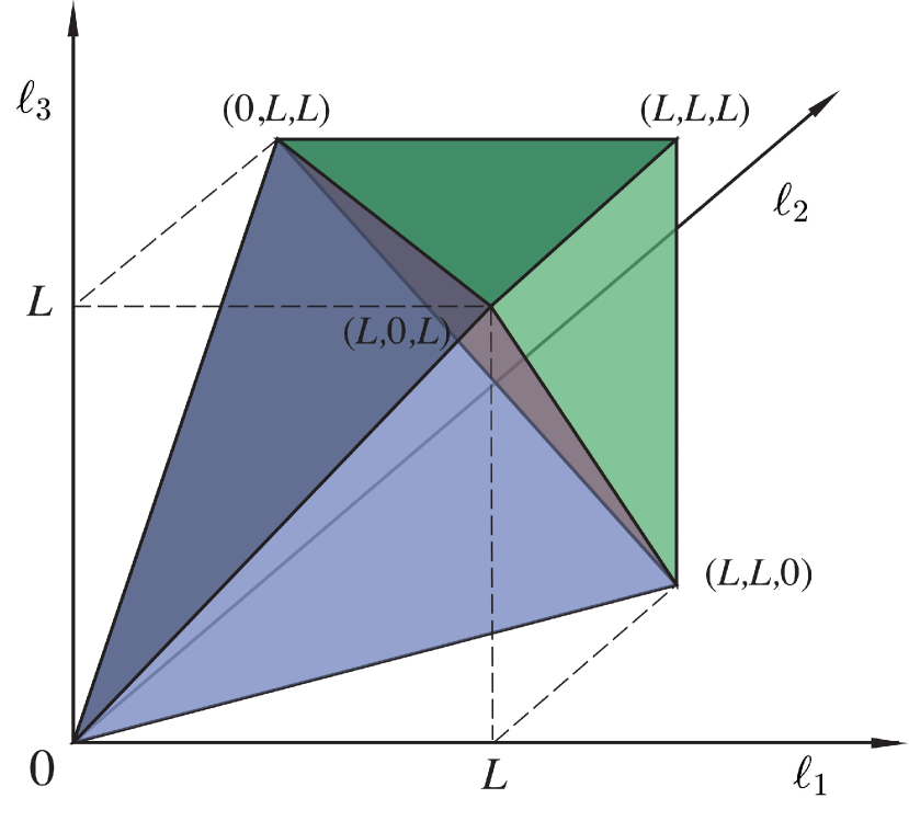
The Wigner- symbol in parentheses enforces rotational symmetry, and allows us to restrict attention to a tetrahedral domain of multipole triplets , satisfying both a triangle condition and a limit given by some maximum resolution (the latter being defined by the finite angular resolution of the experiment under study). This three-dimensional domain of allowed multipoles, sometimes referred to in the following as a “tetrapyd”, is illustrated in Fig. 1 and it is explicitly defined by
| (32) | |||
Here, is the isotropic subset of the full space of bispectra, denoted by .
One can also define an alternative rotationally-invariant reduced bispectrum in the following way:
| (33) |
Note that this is equal to times the angle-averaged bispectrum as defined in the literature. From Eqs. (24) and (25), and the fact that the sum over all of the Wigner- symbol squared is equal to 1, it is easy to see that is related to the reduced bispectrum by
| (34) |
The interest in this bispectrum is that it can be estimated directly from maximally-filtered maps of the data:
| (35) |
where the filtered maps are defined as:
| (36) |
This can be seen by replacing the in Eq. (33) by its estimate and then using Eq. (25) to rewrite the Wigner symbol in terms of a Gaunt integral, which in its turn is expressed as an integral over the product of three spherical harmonics.
3.2 CMB bispectrum estimators
The full bispectrum for a high-resolution map cannot be evaluated explicitly because of the sheer number of operations involved, , as well as the fact that the signal will be too weak to measure in individual multipoles with any significance. Instead, we essentially use a least-squares fit to compare the bispectrum of the observed CMB multipoles with a particular theoretical bispectrum . We then extract an overall “amplitude parameter” for that specific template, after defining a suitable normalization convention so that we can write , where is defined as the value of the theoretical bispectrum ansatz for .
Optimal 3-point estimators, introduced by Heavens (1998) (see also Gangui & Martin 2000a), are those which saturate the Cramér-Rao bound. Taking into account the fact that instrument noise and masking can break rotational invariance, it has been shown that the general optimal estimator can be written as (Babich 2005; Creminelli et al. 2006; Senatore et al. 2010; Verde et al. 2013):
| (37) | ||||
where is the inverse of the covariance matrix and is a suitable normalization chosen to produce unit response to .
In the expression of the optimal estimator above we note the presence of two contributions, one (hereafter defined the “cubic term” of the estimator) is cubic in the observed and correlates the bispectrum of the data to the theoretical fitting template , while the other is linear in the observed (hereafter, the “linear term”), which is zero on average. In the rotationally-invariant case the linear term is proportional to the monopole in the map, which has been set to zero, so in this case the estimator simply reduces to the cubic term. However, when rotational invariance is broken by realistic experimental features such as a Galactic mask or an anisotropic noise distribution, the linear term has an important effect on the estimator variance. In this case, the coupling between different would in fact produce a spurious increase in the error bars (coupling of Fourier modes due to statistical anisotropy can be “misinterpreted” by the estimator as NG). The linear term correlates the observed to the power spectrum anisotropies and removes this effect, thus restoring optimality (Creminelli et al. 2006; Yadav et al. 2008, 2007).
The actual problem with Eq. (37) is that its direct implementation to get an optimal estimator would require measurement of all the bispectrum configurations from the data. As already mentioned at the beginning of this section, the computational cost of this would scale like and be totally prohibitive for high-resolution CMB experiments. Even taking into account the constraints imposed by isotropy, the number of multipole triples is of the order of at Planck resolution, and the number of different observed bispectrum configurations is of the order of . For each of them, costly numerical evaluation of the Wigner symbol is also required. This is completely out of reach of existing supercomputers. It is then necessary to find numerical solutions that circumvent this problem and in the following subsections we will show how the different estimators used for the Planck data analysis address this challenge. Before entering into a more accurate description of these different methods, we would like however to stress again that they are all going to be different implementations of the optimal estimator defined by Eq. (37); therefore they are conceptually equivalent and expected to produce results that are in very tight agreement. This will later on allow for stringent validation tests based on comparing different pipelines. On the other hand, it will soon become clear that the different approaches that we are going to discuss also open up a range of additional applications beyond simple estimation for standard bispectra. Such applications include, for example, full bispectrum reconstruction (in a suitably smoothed domain), tests of directional dependence of , and other ways to reduce the amount of data, going beyond simple single-number estimation. So different methods will also provide a vast range of complementary information.
Another important preliminary point, to notice before discussing different techniques, is that none of the estimators in the following sections implement exactly Eq. (37), but a slightly modified version of it. In Eq. (37) the CMB multipoles always appear weighted by the inverse of the full covariance matrix. Inverse covariance filtering of CMB data at the high angular resolutions achieved by experiments like WMAP and Planck is another very challenging numerical issue, which was fully addressed only recently (Smith et al. 2009; Komatsu et al. 2011; Elsner & Wandelt 2013). For our analyses we developed two independent inverse-covariance filtering pipelines. The former is based on an extension to Planck resolution of the algorithm used for WMAP analysis (Smith et al. 2009; Komatsu et al. 2011); the latter is based on the algorithm described in Elsner & Wandelt (2013). However, detailed comparisons interestingly showed that our estimators perform equally well (i.e., they saturate the Cramér-Rao bound) if we approximate the covariance matrix as diagonal in the filtering procedure and we apply a simple diffusive inpainting procedure to the masked areas of the input CMB maps. A more detailed description of our inpainting and Wiener filtering algorithms can be found in Sect. 3.3.
In the diagonal covariance approximation, the minimum variance estimator is obtained by making the replacement in the cubic term and then including the linear term that minimizes the variance for this class of cubic estimator (Creminelli et al. 2006). This procedure leads to the following expression:
| (38) |
where the tilde denotes the modification of and to incorporate instrument beam and noise effects, and indicates that the multipoles are obtained from a map that was masked and preprocessed through the inpainting procedure detailed in Sect. 3.3. This means that
| (39) |
where denotes the experimental beam, and is the noise power spectrum. For simplicity of notation, in the following we will drop the tilde and always assume that beam, noise and inpainting effects are properly included.
Using Eqs. (33) and (34) we can rewrite Eq. (3.2) in terms of the bispectrum :
| (40) |
In the above expression, is the theoretical template for (with ) and denotes the observed bispectrum (the cubic term), extracted from the (inpainted) data using Eq. (35). is the linear correction, also computed using Eq. (35) by replacing two of the filtered temperature maps by simulated Gaussian ones and averaging over a large number of them (three permutations). The variance in the inverse-variance weights is given by (remember that these should be viewed as being the quantities with tildes, having beam and noise effects included) with a permutation factor ( when all are equal, when two are equal, and otherwise). Both Eqs. (3.2) and (40) will be used in the following. Eq. (3.2) will provide the starting point for the KSW, skew- and modal estimators, while Eq. (40) will be the basis for the binned and wavelets estimators.
Next, we will describe in detail the different methods, and show how they address the numerical challenge posed by the necessity to evaluate a huge number of bispectrum configurations. To summarize loosely: the KSW estimator, the skew- approach and the separable modal methodology achieve massive reductions in computational costs by exploiting structural properties of , e.g., separability. On the other hand, the binned bispectrum and the wavelet approaches achieve computational gains by data compression of .
3.2.1 The KSW estimator
To understand the rationale behind the KSW estimator (Komatsu et al. 2005, 2003; Senatore et al. 2010; Creminelli et al. 2006; Yadav et al. 2008, 2007; Yadav & Wandelt 2008; Smith & Zaldarriaga 2011), assume that the theoretical reduced bispectrum can be exactly decomposed into a separable structure, e.g., there exist some sequences of functions such that we can approximate as
| (41) | |||||
where is a radial coordinate. This assumption is fulfilled in particular by the local shape (Komatsu & Spergel 2001; Babich et al. 2004), with and involving integrals of products of spherical Bessel functions and CMB radiation transfer functions. Let us consider the optimal estimator of Eq. (3.2) and neglect for the moment the linear part. Exploiting Eq. (41) and the factorizability property of the Gaunt integral (Eq. (25)), the cubic term of the estimator can be written as:
| (42) |
where
| (43) |
and
| (44) |
From the formulae above we see that the overall triple integral over all the configurations has been factorized into a product of three separate sums over different . This produces a massive reduction in computational time, as the problem now scales like instead of the original . Moreover, the bispectrum can be evaluated in terms of a cubic statistic in pixel space from Eq. (42), and the functions , are obtained from the observed by means of Fast Harmonic Transforms.
It is easy to see that the linear term can be factorized in analogous fashion. Again considering the local shape type of decomposition of Eq. (41), it is possible to find:
| (45) |
where denotes a Monte Carlo (MC) average over simulations accurately reproducing the properties of the actual data set (basically we are taking a MC approach to estimate the product between the theoretical bispectrum and the covariance matrix appearing in the linear term expression).
The estimator can be finally expressed as a function of and :
| (46) |
Whenever it can be applied, the KSW approach makes the problem of estimation computationally feasible, even at the high angular resolution of the Planck satellite. One important caveat is that factorizability of the shape, which is the starting point of the method, is not a general property of theoretical bispectrum templates. Strictly speaking, only the local shape is manifestly separable. However, a large class of inflationary models can be extremely well approximated by separable equilateral and orthogonal templates (Babich et al. 2004; Creminelli et al. 2006; Senatore et al. 2010). The specific expressions of cubic and linear terms are of course template-dependent, but as long as the template itself is separable their structure is analogous to the example shown in this Section, i.e., they can be written as pixel space integrals of cubic products of suitably-filtered CMB maps (involving MC approximations of the covariance for the linear term). For a complete and compact summary of KSW implementations for local, equilateral and orthogonal bispectra see Komatsu et al. (2009, Appendix).
3.2.2 The Skew- Extension
The skew- statistics were introduced by Munshi & Heavens (2010) to address an issue with estimators such as KSW which reduce the map to an estimator of for a given type of NG. This level of data compression, to a single number, has the disadvantage that it does not allow verification that a NG signal is of the type which has been estimated. KSW on its own cannot tell if a measurement of of given type is actually caused by NG of that type, or by contamination from some other source or sources. The skew- statistics perform a less radical data compression than KSW (to a function of ), and thus retain enough information to distinguish different NG signals. The desire to find a statistic which is able to fulfil this rôle, but which is still optimal, drives one to a statistic which is closely related to KSW, and indeed reduces to it when the scale-dependent information is not used. A further advantage of the skew- is that it allows joint estimation of the level of many types of NG simultaneously. This requires a large number of simulations for accurate estimation of their covariance matrix, and they are not used in this role in this paper. However, they do play an important part in identifying which sources of NG are clearly detected in the data, and which are not.
We define the skew- statistics by extending from KSW, as follows: from Eq. (42), the numerator can be rewritten as
| (47) |
where
| (48) | |||||
and
| (49) | |||||
The skew- approach allows for the full implementation of the KSW procedure, when the sum in Eq. (47) is fully evaluated; furthermore, it allows for extra degrees of flexibility, e.g., by restricting the sum to subsets of the multipole space, which may highlight specific features of the NG signal. Each form of NG considered has its own , hence its own set of skew-, denoted , and we have chosen to illustrate here with the local form, but as with KSW the method can be extended to other separable shapes, and some skew- do not involve integrals, such as the ISW-lensing skew statistic. Note that in this paper we do not fit the directly, but instead we estimate the NG using KSW, and then verify (or not) the nature of the NG by comparing the skew- with the theoretical expectation. No further free parameters are introduced at this stage. This procedure allows investigation of KSW detections of NG of a given type, assessing whether or not they are actually due to NG of that type.
3.2.3 Separable Modal Methodology
Primordial bispectra need not be manifestly separable (like the local bispectrum), or be easily approximated by separable ad hoc templates (equilateral and orthogonal), so the direct KSW approach above cannot be applied generically (nor to late-time bispectra). However, we can employ a highly-efficient generalization by considering a complete basis of separable modes describing any late-time bispectrum (see Fergusson & Shellard 2007; Fergusson et al. 2010a), as applied to WMAP-7 data for a wide variety of separable and non-separable bispectrum models (Fergusson et al. 2012). See also Planck Collaboration XXIII (2013) and Planck Collaboration XXV (2013). We can achieve this by expanding the signal-to-noise-weighted bispectrum as
| (50) |
where the (non-orthogonal) separable modes are defined by
| (51) |
It is more efficient to label the basis as , with the subscript representing an ordering of the products (e.g., by distance ). The are any complete basis functions up to a given resolution of interest and they can be augmented with other special functions adapted to target particular bispectra. The modal coefficients in the bispectrum of Eq. (50) are given by the inner product of the weighted bispectrum with each mode
| (52) |
where the modal transformation matrix is
| (53) |
In the following, the specific basis functions we employ include either weighted Legendre-like polynomials or trigonometric functions. These are combined with the Sachs-Wolfe local shape and the separable ISW shape in order to obtain high correlations to all known bispectrum shapes (usually in excess of 99%).
Substituting the separable mode expansion of Eq. (50) into the estimator and exploiting the separability of the Gaunt integral (Eq. (25)), yields
| (54) |
where the represent versions of the original CMB map filtered with the basis function (and the weights ), that is,
| (55) |
The maps incorporate the same mask and a realistic model of the inhomogeneous instrument noise; a large ensemble of these maps, calculated from Gaussian simulations, is used in the averaged linear term in the estimator of Eq. (3.2.3), allowing for the subtraction of these important effects. Defining the integral over these convolved product maps as cubic and linear terms respectively,
| (56) | ||||
| (57) |
the estimator reduces to a simple sum over the mode coefficients
| (58) |
where . The estimator sum in Eq. (58) is now straightforward to evaluate because of separability, since it has been reduced to a product of three sums over the observational maps (Eq. (3.2.3)), followed by a single 2D integral over all directions (Eq. (56)). The number of operations in evaluating the estimator sum is only .
For the purposes of testing a wide range inflationary models, we can also define a set of primordial basis functions for wavenumbers satisfying the triangle condition (again we will order the with ). This provides a separable expansion for an arbitrary primordial shape function , that is,
| (59) |
Using the same transfer functions as in the KSW integral (42), we can efficiently project forward each separable primordial mode to a corresponding late-time solution (essentially the projected CMB bispectrum for ). By finding the inner product between these projected modes and the CMB basis functions , we can obtain the transformation matrix (Fergusson et al. 2010a, b)
| (60) |
which projects the primordial expansion coefficients to late-time:
| (61) |
When is calculated once we can efficiently convert any given primordial bispectrum into its late-time CMB bispectrum counterpart using Eq. (50). We can use this to extend the KSW methodology and to search for the much broader range of primordial models beyond local, equilateral and orthogonal, having validated on these standard shapes.
3.2.4 Binned Bispectrum
In the binned bispectrum approach (Bucher et al. 2010), the computational gains are achieved by data compression of the observed . This is quite feasible, because like the power spectrum the bispectrum is a rather smooth function, with features on the scale of the acoustic peaks. In this way one obtains an enormous reduction of the computational resources needed at the cost of only a tiny increase in variance (typically ).
More precisely, the following statistic is considered,
| (62) |
where the are intervals (bins) of multipole values , for , with and , and the other bin boundaries chosen in such a way as to minimize the variance of . The binned bispectrum is then obtained by using instead of in the expression for the sample bispectrum of Eq. (35), to obtain:
| (63) |
The linear term is binned in an analogous way, and the theoretical bispectrum template and variance are also binned by summing them over the values of inside the bin. Finally is determined using the binned version of Eq. (40), i.e., by replacing all quantities by their binned equivalent and replacing the sum over by a sum over bin indices . An important point is that the binned bispectrum estimator does not mix the observed bispectrum and the theoretical template weights until the very last step of the computation of (the final sum over bin indices). Thus, the (binned) bispectrum of the map is also a direct output of the code. Moreover, one can easily study the -dependence of the results by omitting bins from this final sum.
The full binned bispectrum allows one to explore the bispectral properties of maps independent of a theoretical model. Binned bispectra have been used to compare component separation maps and single-frequency maps dominated by foregrounds, as presented in Sects. 3.4.2 and 7. In its simplest implementation, which is used in this paper, the binned estimator uses top-hat filters in harmonic space, which makes the Gaussian noise independent between different bins; however, slightly overlapping bins could be used to provide better localization properties in pixel space. In this sense the binned estimator is related to the wavelet estimators, which we discuss below.
3.2.5 Wavelet estimator
Wavelet methods are well-established in the CMB literature and have been applied to virtually all areas of the data analysis pipeline, including map-making and component separation, point source detection, search for anomalies and anisotropies, cross-correlation with large scale structure and the ISW effect, and many others (see for instance Antoine & Vandergheynst 1998, Martínez-González et al. 2002, Cayon et al. 2003, McEwen et al. 2007a, Pietrobon et al. 2006, Starck et al. 2006, McEwen et al. 2007b, Cruz et al. 2007, Faÿ et al. 2008, Feeney et al. 2011, Geller & Mayeli 2009a, Geller & Mayeli 2009b, Starck et al. 2010, Scodeller et al. 2011, Fernández-Cobos et al. 2012). These methods have the advantage of possessing localization properties both in real and harmonic space, allowing the effects of masked regions and anisotropic noise to be dealt with efficiently.
In terms of the current discussion, wavelets can be viewed as a way to compress the sample bispectrum vector by a careful binning scheme in the harmonic domain. See also Planck Collaboration XXIII (2013). In particular, the wavelet bispectrum can be rewritten as
| (64) |
where
| (65) |
Here is the position on the sky at which the wavelet coefficient is evaluated and is is the dispersion of the wavelet coefficient map for the scale . The filters can be seen as the coefficients of the expansion into spherical harmonic of the Spherical Mexican Hat Wavelet (SMHW) filter
| (66) |
Here is a normalizing constant and represents the distance between and , evaluated on the stereographic projection on the tangent plane at ; is the corresponding angular distance, evaluated on the spherical surface.
The implementation of the linear-term correction can proceed in analogy with the earlier cases. However, note that, in view of the real-space localization properties of the wavelet filters, the linear term here is smaller than for KSW and related approaches, although not negligible. Moreover, it can be well-approximated by a term-by-term sample-mean subtraction for the wavelet coefficients, which allows for a further reduction of computational costs. Further details can be found in Curto et al. (2011a, b, 2012); Regan et al. (2013) (see also Lan & Marinucci 2008; Rudjord et al. 2009; Pietrobon et al. 2009, 2010; Donzelli et al. 2012 for related needlet-based procedures).
3.3 Wiener filtering
As discussed in Sect. 3.2, the bispectrum estimator requires, in principle, inverse covariance filtering of the data to achieve optimality (equivalent to Wiener filtering up to a trivial multiplication by the inverse of the signal power spectrum).
We have used the iterative method of Elsner & Wandelt (2013) for Wiener filtering simulations and data. The algorithm makes use of a messenger field, introduced to mediate between the pixel space and harmonic space representation, where noise and signal properties can be specified most directly. Since the Wiener filter is the maximum a posteriori solution, we monitor the of the current solution as a convergence diagnostics. We terminate the algorithm as soon as the improvement in the posterior between two consecutive steps has dropped below a threshold of , where is the standard deviation of -distributed variables with a number of degrees of freedom given by the number of observed pixels. Results of this method have been cross-validated using an independent conjugate gradient inversion algorithm with multi-grid preconditioning, originally developed for the analysis of WMAP data in Smith et al. (2009). Applying this estimator to simulations pre-processed using the above mentioned algorithms yielded optimal error bars as expected.
However, we found that optimal error bars could also be achieved for all shapes using a much simpler diffusive inpainting pre-filtering procedure that can be described as follows: all masked areas of the sky (both Galactic and point sources) are filled in with an iterative scheme. Each pixel in the mask is filled with the average of all surrounding pixels, and this is repeated times over all masked pixels (we checked on simulations that convergence of all estimates was achieved with iterations). Note that the effect of this inpainting procedure, especially visible for the Galactic mask, is effectively to apodize the mask, reproducing small-scale structure near the edges and only large-scale modes in the interior. This helps to prevent propagating any sharp-edge effects or lack of large-scale power in the interior of the mask to the unmasked regions during harmonic transforms.
Any bias and/or excess variance arising from the inpainting procedure were assessed through MC validation (see Sect. 6) and found to be negligible. Since the inpainting procedure is particularly simple to implement, easily allows inclusion of realistic correlated-noise models in the simulations, and retains optimality, we chose inpainting as our data filtering procedure for the analysis.
3.4 CMB bispectrum reconstruction
3.4.1 Modal bispectrum reconstruction
Modal and related estimators can be used to reconstruct the full bispectrum from the modal coefficients obtained from map filtering with the separable basis functions (Eq. (56)) (Fergusson et al. 2010a). It is easy to show that the expectation value for (or equivalently ) for an ensemble of non-Gaussian maps generated with a CMB bispectrum shape given by (Eq. (52)) (with amplitude ) is
| (67) |
where is defined in Eq. (3.2.3). Hence, we expect the best fit coefficients for a particular realization to be given by the s themselves (for a sufficiently large signal). Assuming that we can extract the coefficients accurately from a particular experiment, we can directly reconstruct the CMB bispectrum using the expansion of Eq. (3.2.3), that is,
| (68) | |||||
| (69) |
where, for convenience, we have also defined orthonormalized basis functions with coefficients and such that . This method has been validated for simulated maps, showing the accurate recovery of CMB bispectra, and it has been applied to the WMAP-7 data to reconstruct the full 3D CMB bispectrum (Fergusson et al. 2012).
To quantify whether or not there is a model-independent deviation from Gaussianity, we can consider the total integrated bispectrum. By summing over all multipoles, we can define a total integrated nonlinearity parameter which, with the orthonormal modal decomposition of Eq. (69) becomes (Fergusson et al. 2012)
| (70) |
where is the normalization for the local model. The expectation value contains more than just the three-point correlator, with contributions from products of the two-point correlators and even higher-order contributions,
| (71) |
Here is the full 6-point function over the unconnected Gaussian part, i.e., the product of 3 . So, for a Gaussian input this recovers an average of 1 per mode. In the non-Gaussian case the leading-order contributions after the Gaussian part are the bispectrum squared and the product of the power spectrum and the trispectrum, which enter at the same order (for additional explanations see Fergusson et al. 2012).
3.4.2 Smoothed binned bispectrum reconstruction
As explained in Sect. 3.2.4, the full binned bispectrum of the maps under study is one of the products of the binned estimator code.
Given the relatively fine binning (about 50 bins up to or ), most of the measurement in any single bin-triplet is noise. If combinations of maps are chosen so that the CMB primordial signal dominates, most of this noise is Gaussian, reflecting the fact that even when , for a particular statistical realization, is almost certainly non-zero. If our goal is to test whether there is any statistically significant signal, then it makes sense to normalize by defining a new field , which is the binned bispectrum divided by its expected standard deviation (computed in the standard way assuming Gaussian statistics). The distribution of in any one bin-triplet is very nearly Gaussian as a result of the central limit theorem, and there is almost no correlation between different bins.
We could study the significance of the extreme values at this fine resolution, but it also makes sense to smooth in order to detect features coherent over a wider range of . If the three-dimensional domain over which the bispectrum is defined (consisting of those triplets in the range satisfying the triangle inequality and parity condition) did not have boundaries, the smoothing would be more straightforward. We smooth with a Gaussian kernel of varying width in , normalized so that the smoothed function in each pixel would be normal-distributed if the input map were Gaussian. In this way, based on the extreme values, it is possible to decide on whether there is a statistically significant NG signal in the map in a “blind” (non-parametric) way.
4 Statistical estimation of the CMB trispectrum
4.1 The squeezed-diagonal trispectrum:
The 4-point function, or equivalently the trispectrum, of the CMB, can also place interesting constraints on inflationary physics. There are several physically interesting “shapes” of the trispectrum (e.g., Huang & Shiu 2006; Byrnes et al. 2006; Fergusson et al. 2010b; Izumi et al. 2012), in analogy to the bispectrum case. In the simplest non-Gaussian models, the CMB bispectrum has larger signal-to-noise than the trispectrum, but there are examples of technically natural models in which the trispectrum has larger signal-to-noise (e.g., Senatore & Zaldarriaga 2011; Baumann & Green 2012; see also Bartolo et al. 2010b). This can happen in models in which the field modulating the fluctuation amplitude is only weakly correlated to the observed large-scale curvature perturbation.
Analysis of the trispectrum is more challenging than that of the bispectrum, due to the increased range of systematic effects and secondary signals which can contribute. For example, gravitational lensing of the CMB generates a many-sigma contribution to the trispectrum, though it has a distinctive anisotropic shape that differs from primordial NG modulated by scalar fields. As an instrumental example, any mismatch between the true covariance of the observed CMB plus noise and the covariance which is assumed in the analysis (due, for example, to mischaracterisation of the pointing, beams, or noise properties) will generally lead to biases in the estimated trispectrum. Due to these challenges, we have deferred a full analysis of the primordial trispectrum to a future paper, and here focus on the simplest squeezed shape that can provide useful constraints on primordial models, .
is most easily understood as measuring the large-scale modulation of small-scale power. The constraints on show that such a modulation must be small if correlated with the temperature. However it is possible for multi-field inflation models to produce squeezed-shape modulations which are uncorrelated with the large-scale curvature perturbations. Such models can be constrained by the trispectrum, conventionally parameterized by in the squeezed-diagonal shape.
For example, consider the case where a small-scale Gaussian curvature perturbation is modulated by another field so that the primordial perturbation is given by
| (72) |
where is a large-scale modulating field (with amplitude ). The large-scale modes of can be measured from the modulation they induce in the small-scale power spectrum. If has a nearly scale-invariant spectrum, the nearly-white cosmic variance noise on the reconstruction dominates on small-scales, so only the very largest modes can be reconstructed (Kogo & Komatsu 2006). A reconstruction of is going to be limited to only very large-scale variations, in which case the scale of the variation is very large compared to the width of the last-scattering surface; i.e., in any particular direction a large-scale modulating field will modulate all small-scale perturbations through the last-scattering surface by approximately the same amount. This approximation is good at the percent level, and can readily be related to the full trispectrum estimator, as discussed in more detail in Pearson et al. (2012, Sect. IV); see also Okamoto & Hu 2002; Munshi et al. 2011; Smidt et al. 2010.
A large-scale power modulation therefore translates directly into a large-scale modulation of the small-scale CMB temperature:
| (73) |
where are the usual small-scale Gaussian CMB temperature anisotropies and is the radial distance to the last-scattering surface. We can quantify the trispectrum as a function of modulation scale by using the power spectrum of the modulation,
| (74) |
As is conventional, we normalize relative to , the power spectrum of the primordial curvature perturbation at the location of the recombination surface. The field is directly observable, but is not, since the curvature perturbation can only be constrained very indirectly on very large scales. We shall therefore give constraints on , which is directly constrained by Planck, but also on for comparison with the inflation literature. Note that corresponds to an modulation.
A general quadratic estimator methodology for reconstructing was developed in Hanson & Lewis (2009), which we broadly follow here. The structure is essentially identical to that for lensing reconstruction (Planck Collaboration XVII 2013), where here instead of reconstructing a lensing potential (or deflection angle), we are reconstructing a scalar modulation field. The quadratic maximum likelihood estimator for the large-scale modulation field (assuming it is small) is given by
| (75) |
where is a quadratic function of the filtered data that can be calculated quickly in real space:
| (76) |
Here is an inverse-variance filtering sky map (which accounts for sky cuts and inhomogeneous noise), and is the lensed . The “mean field” can be estimated from simulations, along with the Fisher normalization that is given by the covariance of . The indices are included here, since we shall be using different sky maps with independent noise to avoid noise biases at the level of modulation field reconstruction. For low and high the reconstruction noise is very nearly constant (white, because each small patch of sky gives a nearly-uncorrelated but noisy estimate of the small-scale power), and the reconstruction is very local.
In practice the inverse-variance filtering is imperfect, the noise cannot be modelled exactly, and the normalizing Fisher matrix evaluated from simulations would be inaccurate. Instead we focus on directly, which is approximately an inverse-variance weighed reconstruction of the modulation, and is manifestly very local in real space (and hence zero in the cut part of the sky). Since the reconstruction noise, which also approximately determines the normalization, is nearly white (constant in ), in real space has an expectation nearly proportional to the underlying modulation outside the mask.
We then define an estimator of the modulation power spectrum
| (77) |
where
| (78) |
is a noise bias for zero signal estimated from simulations. The normalization is the analytic ideal full-sky normalization which is very close to a constant, and is a calibration factor determined from with-signal simulations. On small scales , but has some scale dependence: it increases towards at at very low . We shall sometimes plot , corresponding to the uncalibrated reconstruction of the power modulation, which is very local in real space.
For each value of the modulation scale , Eq. (77) defines a separate estimator for
| (79) |
We can combine estimators from all by constructing
| (80) |
where and is the covariance of from simulations with . On the full-sky the estimators from each would be independent, but the mask introduces significant coupling between the very low multipoles and this form of the estimator allows us to account for this. In the full-sky uncorrelated approximation, with a nearly scale-invariant primordial spectrum and using the whiteness of the reconstruction noise, the estimator for simplifies to (Pearson et al. 2012)
| (81) |
where . This result does not require many simulations to estimate the covariance accurately for inversion, and is typically expected to give very similar results with an error bar that is less than larger. We calculate both as a cross-check, but report results for because it is more robust, and in our simulation results actually has slightly lower tails (though larger variance). Mean fields and the bias are estimated in all cases from 1000 zero- simulations, and the mask used retains about of the sky.
If there is a nearly scale-invariant signal, so as expected in most multi-field inflation models, the contributions fall rapidly , as expected when measuring a scale-invariant signal that has large white reconstruction noise. The signal is therefore on very large scales, with typically half the Fisher signal in the dipole modulation and of the signal at , justifying the squeezed approximations used. We use for the estimators, which includes almost all of the signal-to-noise but avoids excessive contamination with the ‘blue’ spectrum of lensing contributions. However, due to the small number of modes involved, the posterior distributions of can have quite broad tails corresponding to the finite probability that all the largest-scale modulation modes just happen to be near zero. To improve constraints on large values it can help to include a larger range of , and we consider up to , which is about the limit of where the approximations are valid.
5 Non-primordial contributions to the CMB bispectrum and trispectrum
In this subsection we present the steps followed to account for and remove the main non-primordial contributions to CMB NG.
5.1 Foreground subtraction
Foreground emission signals in the microwave bands have a strong non-Gaussian signature. Therefore any residual emission in the CMB data can give a spurious apparent primordial NG detection. In our analysis we considered Planck CMB foreground-cleaned maps created using several independent techniques, as described in Planck Collaboration XII (2013): explicit parametrization and fitting of foregrounds in real space (Commander-Ruler, C-R) (Eriksen et al. 2006, 2008); Spectral Matching of foregrounds implementing Independent Component Analysis (SMICA) (Delabrouille et al. 2003; Cardoso et al. 2008); Internal Linear Combination (Needlet Internal Linear Combination, (NILC) (Delabrouille et al. 2009); and Internal Template Fitting (SEVEM) (Fernández-Cobos et al. 2012). These and other techniques underwent a pre-launch testing phase (Leach et al. 2008). Each method provides a Planck CMB foreground-cleaned map with a confidence mask, which defines the trusted cleaned region of the sky; an estimate of the noise in the output CMB map obtained from half-ring difference maps; and an estimate of the beam transfer function of the processed map. The resolution reaches 5 arcminutes. In addition a union of all the confidence masks, denoted as U73, is provided. Channels from both the Low Frequency Instrument (LFI, Planck Collaboration II 2013) and the High Frequency Instrument (HFI, Planck Collaboration VI 2013) of Planck are used to achieve each of the reconstructed CMB templates. The validation of CMB reconstruction through component separation is based on the inspection of several observables, as explained in detail in Planck Collaboration XII (2013): the two-point correlation function and derived cosmological parameters; indicators of NG including the results presented in the present paper; and cross-correlation with known foreground templates. Based on various figures-of-merit, the foreground cleaning techniques performed comparably well (Planck Collaboration XII 2013).
In order to test foreground residuals a battery of simulations is required. In the simulations the foreground emission was modelled with the pre-launch version of the Planck Sky Model (PSM), based on observations of the emission from our own Galaxy and known extra-Galactic sources, largely in the radio and infrared bands. The PSM is described in Delabrouille et al. (2012) and includes models of CMB (including a dipole), diffuse Galactic emissions (synchrotron, free-free, thermal dust, Anomalous Microwave Emission and CO molecular lines), emission from compact objects (thermal SZ effect, kinetic SZ effect, radio sources, infrared sources, correlated far-infrared background and ultra-compact H ii regions). The sky model includes total intensity as well as polarization, which was not used in this paper.
The PSM has been used to create the sixth round of Full Focal Plane (FFP6) simulations, a set of simulations for the 2013 data release based on detailed models of the sky and instrument (e.g., noise properties, beams, satellite pointing and map-making process), consisting of both Gaussian and non-Gaussian CMB realizations. A description of the FFP6 simulations can be found in Appendix A (see Planck Collaboration ES (2013) for details). The FFP6 set has been used to test and validate the component separation algorithms employed in Planck and to establish uncertainties on the outputs (Planck Collaboration XII 2013). We will also use FFP6 simulations in the next Sections in order to validate our analysis (see Sects. 6, 7, 8).
5.2 The Integrated Sachs-Wolfe-lensing bispectrum
One of the most relevant mechanisms that can generate NG from secondary CMB anisotropies is the coupling between weak lensing and the ISW (Sachs & Wolfe 1967) effect. This is in fact the leading contribution to the CMB secondary bispectrum with a blackbody frequency dependence (Goldberg & Spergel 1999; Verde & Spergel 2002; Giovi et al. 2005).
| ISW-lensing bias Shape . SMICA NILC SEVEM C-R Local . 7.1 7.0 7.1 6.0 Equilateral . 0.4 0.5 0.4 1.4 Orthogonal . 22 21 21 19 |
| ISW-lensing amplitude Method . SMICA NILC SEVEM C-R KSW . 0.81 0.31 0.85 0.32 0.68 0.32 0.75 0.32 Binned . 0.91 0.37 1.03 0.37 0.83 0.39 0.80 0.40 Modal . 0.77 0.37 0.93 0.37 0.60 0.37 0.68 0.39 |
Weak lensing of the CMB is caused by gradients in the matter gravitational potential that distorts the CMB photon geodesics. The ISW on the other hand arise because of time-varying gravitational potentials due to the linear and nonlinear growth of structure in the evolving Universe. Both the lensing and the ISW effect are then related to the matter gravitational potential and thus are correlated phenomena. This gives rise to a non-vanishing 3-point correlation function. Furthermore, lensing is related to nonlinear processes which are therefore non-Gaussian. A detailed description of the signal, which accounts also for the contribution from the early-ISW effect, can be found in Lewis (2012).
The ISW-lensing bispectrum takes the form:
| (82) |
where P, L, and ISW indicate primordial, lensing and ISW contributions respectively. This becomes
| (83) |
where is the Gaunt integral and is the reduced bispectrum given by
| (84) |
Here is the lensed CMB power spectrum and is the ISW-lensing cross-power spectrum (Lewis 2012; Goldberg & Spergel 1999; Verde & Spergel 2002; Cooray & Hu 2000) that expresses the statistical expectation of the correlation between the lensing and the ISW effect.
As shown in Hanson et al. (2009b), Mangilli & Verde (2009), and Lewis et al. (2011), the ISW-lensing bispectrum can introduce a contamination in the constraints on primordial local NG from the CMB bispectrum. Both bispectra are maximal for squeezed or nearly squeezed configurations. The bias on a primordial (e.g., local) due to the presence of the ISW-lensing cross correlation signal is
| (85) |
with
| (86) |
where and refer respectively to the ISW-lensing and the primordial bispectrum, and is defined below Eq. (40).
The bias in the estimation of the three primordial from Planck is given in Table 1. As one can see, taking into account the statistical error bars shown, e.g., in Table 8, the local shape is most affected by this bias (at the level of more than ), followed by the orthogonal shape (at the level of about ), while the equilateral shape is hardly affected. In this paper we have taken into account the bias reported in Table 1 by subtracting it from the measured .888See Kim et al. (2013) for other debiasing techniques.
The results for the amplitude of the ISW-lensing bispectrum from the different foreground-cleaned maps are given in Table 2. It should be noted that the binned and modal estimators are less correlated to the exact template for the ISW-lensing shape than they are for the primordial shapes, hence their larger error bars compared to KSW (which uses the exact template by construction (Mangilli et al. 2013)). The conclusion is that we detect the ISW-lensing bispectrum at a value consistent with the fiducial value of 1, at a significance level of (taking the SMICA-KSW value as reference). For details about comparisons between different estimators and analysis of the data regarding primordial shapes we refer the reader to Sects. 6 and Sect. 7.
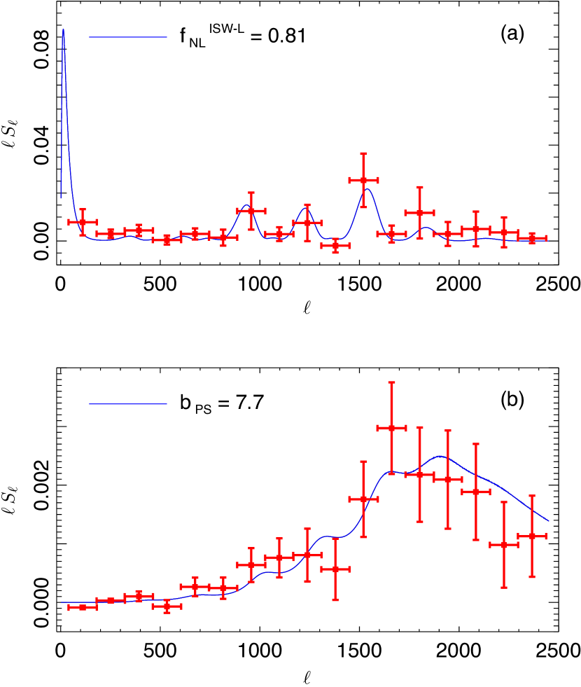
We show for the SMICA map in the top figure of Fig. 2 the measured skew- spectrum (see Sect. 3.2.2) for optimal detection of the ISW-lensing bispectrum, along with the best-fitting estimates of from the KSW method for different values of . It should be noted that the skew- spectrum is not a fit to the KSW data points; its shape is fully fixed by the template under consideration, with only the overall amplitude as a free parameter. Hence the agreement between the curve and the points is good evidence that KSW is really detecting the ISW-lensing effect and not some other source of NG. Note that point sources, at the level determined by their own skew-spectrum, do not contribute significantly to the ISW-lensing statistic). See Planck Collaboration XVII (2013), Planck Collaboration XIX (2013) for further information about the detection by Planck of the ISW-lensing signal.
5.3 Point-sources bispectrum
Extra-Galactic point sources at Planck frequencies are divided into two broad categories: radio sources with synchrotron and/or free-free emission; and infrared galaxies with thermal emission from dust heated by young stars. Radio sources are dominant at central CMB frequencies up to 143 GHz, and can be considered unclustered (Toffolatti et al. 1998; González-Nuevo et al. 2005). Hence their bispectrum is constant and is related to their number counts as
| (87) |
with the flux density, the number counts per steradian, the flux cut and the conversion factor from flux to relative temperature elevation, depending on the frequency and instrumental bandpass.
Infrared galaxies become important at higher frequencies, 217GHz and above, and are highly clustered in dark matter halos, which enhances their bispectrum on large angular scales (Lacasa et al. 2012; Curto et al. 2013). However, in the Planck context it was shown by Lacasa & Aghanim (2012) that the IR bispectrum is more than 90% correlated with the Poissonian template of the radio sources. So a joint estimation of with a Poissonian bispectrum template will essentially account for the IR signal, and provide quasi-identical values compared to an analysis accounting for the IR bispectrum template. Indeed, in our final optimal bispectrum constraints for primordial shapes, we will account for the potential contamination from point sources by jointly fitting primordial and Poisson templates to the data.
Our final measured point-source bispectrum amplitudes from the data are reported in Table 3. The amplitude is expressed in dimensionless units, i.e., it has been divided by the appropriate power of the monopole temperature , and has been multiplied by . As shown in Sect. 8.1, the Poisson template is the only one that still evolves significantly between and . This explains the differences between the values of the KSW and binned (that use ) and the modal (that uses ) estimators. It has been shown that for the same value of all three estimators agree very well.
We finally conclude from Table 3 that we detect the point-source bispectrum with high significance in the SMICA, NILC, and SEVEM cleaned maps, while it is absent from the C-R cleaned map. The measured skew- spectrum of the SMICA map in the bottom figure of Fig. 2 gives further evidence that the NG from foreground point sources is convincingly detected. The only degree of freedom in this plot is the amplitude, which is not set by a direct fit to the skew-, but rather is estimated by KSW. As a result, the good agreement with the shape of this skew- spectrum is powerful evidence that there is NG from point sources. However, this still turns out to be a negligible contaminant for primordial studies, due to the very low correlation between the Poisson bispectrum and the primordial shapes.
| Point source bispectrum amplitude/ Method . SMICA NILC SEVEM C-R KSW. 7.7 1.5 9.2 1.7 7.6 1.7 1.1 5.1 Binned. 7.7 1.6 8.2 1.6 7.5 1.7 0.9 4.8 Modal. 10 3 11 3 10 3 0.5 6 |
5.4 Non-primordial contributions to the trispectrum
The main non-instrumental source of non-primordial signal is the kinematic modulation dipole due to the peculiar velocity of the earth, , whose magnitude is (Challinor & van Leeuwen 2002; Kosowsky & Kahniashvili 2011; Amendola et al. 2011). If data are used to constrain using the dipole modulation (which shrinks the Fisher error by a factor of two relative to starting at ), the dipole-induced signal must be subtracted, since its modulation reconstruction has signal-to-noise larger than unity at Planck resolution. Confirmation that this signal is detected with the expected magnitude and direction is a good test of our methodology. The dipole signal seen by Planck is studied in detail in Planck Collaboration XXVII (2013), so we only summarize the key points here.
The local Doppler effect modulates the observed CMB temperature by at leading order, so that . The spectrum in each direction remains a blackbody, but the relative response in the intensity at the observed Planck frequencies is however frequency dependent. The effective thermodynamic fractional temperature anisotropy at each frequency for zero peculiar velocity is defined by
| (88) |
With peculiar velocity the temperature depends on the second order term , so expanding the Planck function to second order then gives a change in the effective small-scale temperature anisotropy from both first and second order terms in the expansion of :
| (89) | |||||
where (and we neglect small second-order non-modulation terms). Thus the anisotropies in the Planck maps have a dipolar modulation given by , where for the frequency bands we use , , and in the direction of CMB dipole. In addition our peculiar velocity induces kinetic aberration, which looks at leading order exactly like a dipole lensing convergence and only projects weakly into the power anisotropy estimator. For constraining both of the expected kinematic signals can be included in the simulations, and hence subtracted in the mean field of the modulation reconstruction.
Secondary effects are dominated by the significant and very blue lensing signal. However unlike for the bispectrum lensing only overlaps with at a small fraction of the error bar as long as only low modulation multipoles are used, where the signal peaks (Pearson et al. 2012). We include lensing in the simulations, so lensing is straightforwardly accounted for in our analysis by its inclusion in the noise bias (Eq. (78)) and mean field.
A variety of instrumental effects can also give a spurious modulation signal if not modelled accurately. In particular the mean field due to anisotropic noise is very large (Hanson et al. 2009a). On the ultra-large scales of interest for , our understanding of the noise is not adequate to calculate accurately and subtract this large signal. Instead, as for the power spectrum estimation, we use cross-map estimators that have no noise mean field on average. Both the noise and most other instrumental effects such as gain variations are expected to produce a signal with approximate symmetry about the ecliptic plane. Our modulation reconstruction methodology is especially useful here, since we can easily inspect the orientation of any signal found; for example a naive treatment of the noise not using cross-maps would give a large apparent quadrupolar modulation signal aligned with the ecliptic, corresponding to percent-level misestimation of the noise mean field from inaccurate noise simulation.
Beam asymmetries are included in the simulation, as described in Planck Collaboration XVII (2013), but their effect is very small, since the modulation we are reconstructing is isotropic.
Since we are reconstructing a modulation of small-scale power, the estimator is totally insensitive to smooth large-scale foregrounds. However large-scale variation in small-scale foreground power can mimic a trispectrum modulation. We project out 857 GHz as a dust template in our inverse-variance filtering procedure, as described in Appendix A of Planck Collaboration XVII (2013), but do not include any other foreground model in the trispectrum analysis. Any unmodelled foreground power variation would increase the signal, so our modelling is sufficient to place a robust upper limit.
6 Validation Tests
The results quoted in this paper have all been cross-validated using multiple bispectrum-based estimators from different groups. Having multiple estimators was extremely useful for the entire analysis, for two main reasons. First, it allowed great improvement in the robustness of the final results. In the early stages of the work the comparison between different independent techniques helped to resolve bugs and other technical issues in the various computer codes, while during the later stages it was very useful to understand the data and find the optimal way of extracting information about the various bispectrum templates. Secondly, besides these cross-checking purposes, different estimators provide also interesting complementary information, going beyond simple estimation. For example, the binned and modal estimators provide a reconstruction of the full bispectrum of the data (smoothed in different domains), the skew- estimator allows monitoring of the contribution to from different sources of NG, the wavelets reconstruction allows directionality tests, and so on.
In this Section we are concerned with the first point above, that is, the use of multiple bispectrum-based pipelines as a way to improve the robustness of the results. For this purpose, a large amount of work was dedicated to the development and analysis of various test maps, in order to validate the estimators. This means not only checking that the various estimators recover the input within the expected errors, but also that the results agree on a map-by-map basis.
The Section is split into two parts. Sect. 6.1 shows results on a set of initially full-sky, noiseless, Gaussian CMB simulations, to which we add, in several steps, realistic complications, including primordial NG, anisotropic coloured noise, and a mask, showing the impact on the results at each step. In Sect. 6.2 we show our results on a set of simulations that mimic the real data as closely as possible (except for the presence of foreground residuals, which will be studied in Sect. 8.4): no primordial NG, but NG due to the ISW-lensing effect; simulated instrumental effects and realistic noise; and simulations passed through the component separation pipelines. In fact these are the FFP6 simulations (see Appendix A) that are used to determine the error bars for the final Planck results.
We present here only a small subset of the large number of validation tests that were performed. For example, we also had a number of “blind challenges”, in which the different groups received a simulated data set with an unknown value of input for a given shape and they had to report their estimated values. In addition different noise models were tested (white vs. coloured and isotropic vs. anisotropic), leading to the conclusion that it is important to make the noise in the estimator calibration as realistic as possible (coloured and anisotropic). We also tested different Galactic and point source masks, with and without inpainting, concluding that it is best to fill in both the point sources and the Galactic mask, using a sufficient number of iterations in our diffusive procedure to entirely fill in the point source gaps, while at the same time only effectively apodizing the Galactic mask (no small-scale structure in its interior). There were also various tests on FFP simulations of Planck data with Gaussian or non-Gaussian CMB and all foregrounds, provided by the PSM (see Appendix A.4). These simulations were tested both before and after they had passed through the component separation pipelines. In all comparison tests the results were consistent with input values and differences between estimators were consistent with theoretical expectations.
6.1 Validation of estimators in the presence of primordial non-Gaussianity
The aim of the first set of validation tests is threefold. First, we want to study the level of agreement from different estimators in ideal conditions (i.e., full-sky noiseless data). The expected scatter between measurements is, in this case, entirely due to the slightly imperfect correlation between weights of estimators that adopt different schemes to approximate the primordial shape templates. For this case the scatter can be computed analytically (see Appendix B for details). We can then verify that our results in ideal conditions match theoretical expectations. This is done in Sect. 6.1.1. Second, we want to make sure that the estimators are unbiased and correctly recover in input for local, equilateral, and orthogonal shapes. This is done in Sects. 6.1.2 and 6.1.3, where a superposition of local, equilateral and orthogonal bispectra is included in the simulations and the three values are estimated both independently and jointly. Finally we want to understand how much the agreement between pipelines in ideal conditions is degraded when we include a realistic correlated noise component and a sky cut, thus requiring the introduction of a linear term in the estimators in order to account for off-diagonal covariance terms introduced by the breaking of rotational invariance. Since we want to study the impact of adding noise and masking separately, we will first work on a set of full-sky maps with noise in Sect. 6.1.2, and then add a mask in Sect. 6.1.3.
The tests were applied to the KSW, binned and modal estimators. These are the bispectrum pipelines used to analyse Planck data in Sect. 7. Our goal for this set of tests is not so much to attain the tightest possible agreement between methods, as it is to address the points summarized in the above paragraph. For this reason the estimator implementations used in this specific Section were slightly less accurate but faster to compute than those adopted for the final data analysis of Sect. 7. The primary difference with respect to the main analysis is that a smaller number of simulations was used to calibrate the linear term (80–100 in these tests, as against 200 or more for the full analysis). For the modal estimator we also use a faster expansion with a smaller number of modes: 300 here versus 600 in the high accuracy version of the pipeline999While most of the modal results in this paper come from the most accurate 600 modes pipeline, a few computationally intensive data validation tests of Sect. 8 also use the fast 300 modes version; therefore the results in this Section also provide a direct validation of the fast modal pipeline. used in Sect. 7. Even with many fewer modes, the modal estimator is still quite accurate: the correlation coefficient for the modal expansion of the local template is , while for the equilateral and orthogonal shapes it is .
6.1.1 Ideal Gaussian simulations
As a basis for the other tests we start with the ideal case, a set of 96 simulations of a full-sky Gaussian CMB, with a Gaussian beam with FWHM 5 arcmin and without any noise, cut off at in our analyses. The independent Fisher matrix error bars in that case are for local NG, for equilateral, and for orthogonal.
Note that this test does not make sense for all estimators, and hence results are not included for all of them. For example, for the binned estimator the optimal binning depends on the noise. While this dependence is not very strong, the difference between no noise and Planck noise is sufficiently large that a completely different binning would have to be used just for this test, going against the purpose of this Section to validate the estimators as used for the data analysis.101010While the binning with 48 bins and used in the validation tests of Sects. 6.1.2 and 6.1.3 is also slightly different from the binning used for the data analysis with 51 bins and , these differences are very small and the binnings have very similar correlation coefficients of 0.99 or more for local and equilateral shapes, and 0.95 for orthogonal.
The purpose here is mostly aimed at checking consistency with the following formula (derived in Appendix B) for the expected scatter (standard deviation) between results of the same map from an exact and an approximate estimator:
| (90) |
Here is the standard deviation of the exact estimator and is the correlation coefficient that gives the correlation of the approximate bispectrum template with the exact one, defined as
| (91) |
where the label “th” denotes the initial bispectrum shape to fit to the data, and “exp” is the approximate expanded one. Note that this formula has been obtained under the simplifying assumptions of Gaussianity, full-sky coverage and homogeneous noise. For applications dealing with more realistic cases we might expect the scatter to become larger, while remaining qualitatively consistent.
The results averaged over the whole set of maps are given in Table 4 for the KSW and modal estimators individually, as well as for their difference. The plane wave modal expansion implemented here achieves about 98% correlation with the separable shapes used by KSW. According to the formula above we then expect a standard deviation of map-by-map differences of order for a given shape, where is the corresponding error bar. Looking at the left-hand side of Table 4, we see that the error bars are 4 for local NG, 50 for equilateral, and 30 for orthogonal. So we predict a standard deviation of map-by-map differences of 0.8, 10 and 6 for local, equilateral, and orthogonal NG, respectively. As one can see from the “Modal-KSW” column, the measurements are in excellent agreement with the theoretical expectation.
|
||||||||||||||||||||||
6.1.2 Non-Gaussian simulations with realistic noise
| Shape . KSW Binned Modal Binned KSW Modal KSW Independent Local . 13.8 5.2 14.1 5.2 14.1 5.3 0.3 2.1 0.4 2.6 Equilateral . 63 57 62 58 64 57 0.9 20 1.0 18 Orthogonal . 52 37 58 40 54 37 6.0 13 2.2 12 Joint Local . 11.7 6.2 12.0 6.6 12.0 6.4 0.2 2.7 0.2 3.2 Equilateral . 31 59 29 61 31 59 1.8 21 0.2 19 Orthogonal . 20 43 22 47 21 42 2.1 16 0.6 15 |
|
||||||||||||||||||||||||||||||||||||||||||||||||||||||||||||||
A set of 96 full-sky non-Gaussian CMB simulations was created according to the process described by Fergusson et al. (2010a), with local , equilateral , and orthogonal . The effect of a 5 arcmin beam was added, as well as realistic coloured and anisotropic noise according to the specifications of the SMICA cleaned map. The independent Fisher matrix error bars in that case are for local, for equilateral, and for orthogonal NG, while the joint ones are respectively , , and .
The results averaged over the whole set are given in Table 5 for the various estimators individually, as well as for the differences with respect to KSW. Compared to the previous case we now deviate from the exact theoretical expectation for two reasons: we include a realistic correlated noise component; and we have NG in the maps. The presence of NG in the input maps will lower the agreement between estimators with respect to the Gaussian case if the correlation between weights is not exactly 100%. This is even more true in this specific case, where NG of three different kinds is present in the input maps and also cross-correlation terms between different expanded shapes are involved (and propagated over in the joint analysis). Moreover, when noise is included the specific modal expansion used for this test is 95% correlated to the separable KSW local shape (so there is a 3% reduction of the correlation compared to the ideal case for the modal local shape); we thus expect a further degradation of the level of agreement for this specific case. Finally, in order to correct for noise effects, a linear term has to be added to the estimators. Since the linear term is obtained by MC averaging over just 80 or 96 simulations in this test (depending on the estimator), MC errors are also adding to the measured differences. Of course the MC error can be reduced by increasing the number of simulations in the linear term sample. We do this for the analysis of the real data and in Sect. 6.2, but it was computationally too expensive for this set of preliminary validation tests, so we decided here to just account for it in the final interpretation of the results.
As a consequence of the above, we can no longer expect the map-by-map differences to follow perfectly the theoretical expectation, obtained in the previous Section in idealized conditions (full-sky, no noise, and Gaussianity). With these caveats in mind, the agreement between different pipelines remains very good, being about in most cases and about for the modal-KSW difference in the local case, which can be easily explained by the fact that this is the set of weights with the lowest correlation (95%, as mentioned above). All estimators are unbiased and recover the correct input values.
|
||||||||||||||||||||||||||||||||||||||||||||||||||
6.1.3 Impact of the mask
To the simulations of Sect. 6.1.2 we now apply the Planck union mask - denoted U73 - masking both the Galaxy and the brightest point sources and leaving 73% of the sky unmasked (Planck Collaboration XII 2013). This is the same mask used to analyse Planck data in Sect. 7. The independent Fisher matrix error bars in that case (taking into account the correction) are for local NG, for equilateral, and for orthogonal, while the joint ones are respectively , , and .
All masked areas of the sky (both Galactic and point sources) are filled in with a simple iterative method. In this simple inpainting method each pixel in the mask is filled with the average of all eight surrounding pixels, and this is repeated 2000 times over all masked pixels. The filling-in helps to avoid propagating the effect of a sharp edge and the lack of large-scale power inside the mask to the unmasked regions during harmonic transforms. This inpainting method is the one that was used to produce all NG results in this paper for methods that need it (KSW, binned and modal).
The results averaged over the whole set of simulations are given in Table 6 for the various estimators individually, as well as for the differences with respect to KSW. The map-by-map results are shown in Fig. 3.
This is the most realistic case we consider in this set of tests. Besides noise, we also include a sky cut and our usual mask inpainting procedure. All the caveats mentioned for the previous case are still valid, and possibly emphasized by the inclusion of mask and inpainting. In the light of this, the agreement is still very good, worsening a bit with respect to the “full-sky + noise” case only for the local measurement, where the mask is indeed expected to have the biggest impact. In the joint analysis all estimators recover the correct input values for the local and orthogonal cases, but all estimators find a value for equilateral NG that is somewhat too low. It is unclear whether this is an effect of masking and inpainting on the equilateral measurement or just a statistical fluctuation for this set of simulations. In any case, this potential bias is small compared to the statistical uncertainty, so that it would not have a significant impact on the final results.
To summarize the results of this Sect. 6.1, we performed an extensive set of validation tests between different estimators using strongly, but not perfectly, correlated primordial NG templates in their weights. The test consisted in comparing the measured by the different estimators for different sets of simulations, on a map-by-map basis. We started from ideal conditions: full-sky Gaussian noiseless maps. In this case we computed a theoretical formula providing the expected standard deviation of the differences, as a function of the correlations between the input NG templates in the different estimators. Our results match this formula very well. In the other two simulation sets we added realistic features (noise, mask and inpainting) and we included a linear combination of local, equilateral and orthogonal NG. First of all we verified that all the pipelines correctly recover the three input values, hence they are unbiased. Moreover, we observed that adding such features produces an expected slight degradation of the level of agreement between different pipelines, that nevertheless remains very good: about – for equilateral and orthogonal NG, and about – for local NG, which is the shape most affected by mask and noise contamination.
6.2 Validation of estimators on realistic Planck simulations
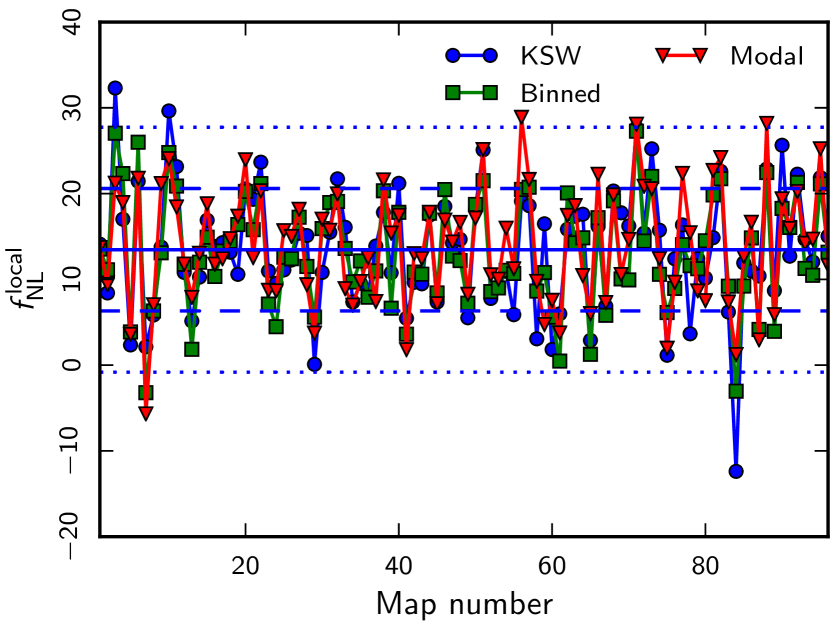
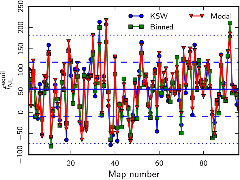
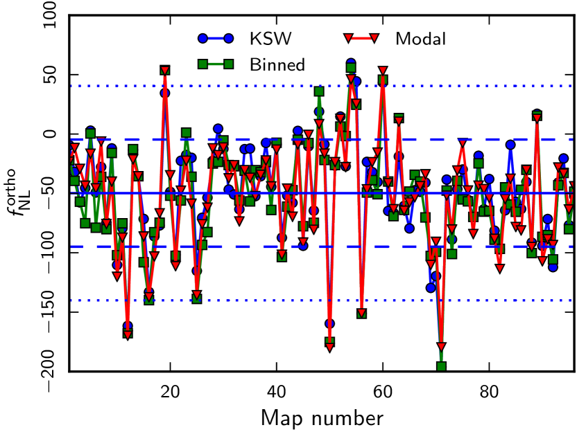
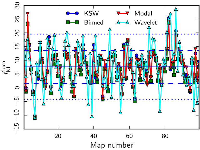
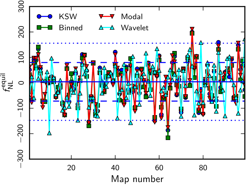
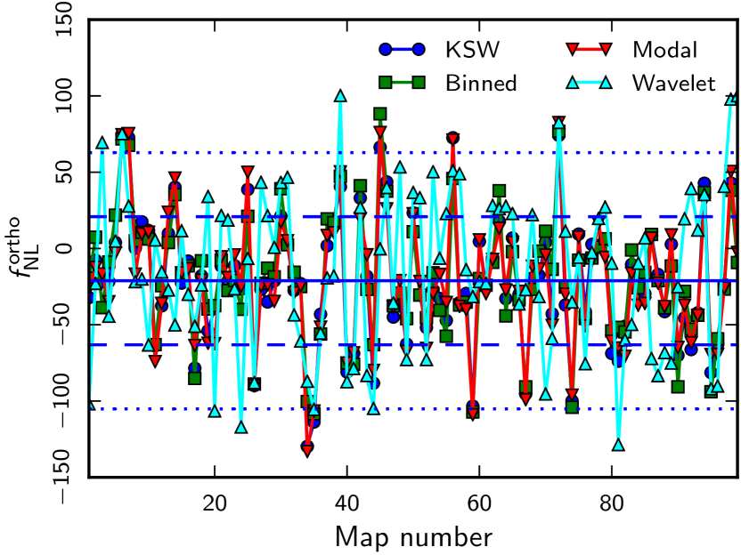
In the tests of the previous Subsection we checked the bias of the estimators and studied their level of agreement, given the correlation between their weights, in the presence of noise and a sky cut. To speed up the computation while still retaining enough accuracy for the purposes of that analysis, we used a relatively small number of maps for linear term calibrations (80–100) and used a smaller number of modes than usual in the modal estimator. In the present Subsection we instead try to simulate as accurately as possible real data analysis conditions. Our goal is to obtain an accurate MC-based expectation of the scatter between different measurements when the pipelines are run on actual Planck maps.
To this aim we use FFP6 simulation maps described in Appendix A. The original FFP6 maps were lensed using the Lenspix algorithm, and processed through the SMICA component separation pipeline. They were then multiplied by the Galactic and point source mask U73 as in the actual analysis, and inpainted as usual. Since our final results show full consistency with Gaussianity for local, equilateral and orthogonal shapes, we do not include any primordial in these maps. We note that although the simulations were passed through SMICA in order to provide a realistic filtering of the data, they did not include any foreground components. The impact of foreground residuals will be studied separately in Sect. 8.4.
The configuration of all bispectrum pipelines was the same as used for the final data analysis, which implies a correlation of or better between the weights of the KSW, binned and modal estimators. Linear terms were calibrated using simulations, after verifying that this number allows accurate convergence for all the shapes. For this test we also included the wavelet bispectrum pipeline described in Sect. 3. Although this last estimator turns out to be about suboptimal and, in its current implementation, less correlated with the primordial templates than the other estimators, it does provide an additional interesting cross-check of our results by introducing another decomposition basis. We thus used it to analyse SMICA data in Sect. 7, while the other three pipelines were used on all maps.
A comparison of the measured map-by-map for all shapes and estimators is shown in Fig. 4. As an overall figure of merit of the level of agreement achieved by different pipelines we take as usual the standard deviation of the map-by-map differences, . Table 7 shows that the final agreement between the three optimal pipelines (KSW, binned, and modal) is close to saturating the ideal bound in Eq. (90) determined by the imperfect correlation of the weights, i.e., it varies from about once to twice for an correlation. This is very consistent with the level of agreement that we find between estimators for the final results from the data, providing a good indication that no spurious NG features are present in the actual data set when compared to our simulations. It should be noted that we found a similarly good level of agreement between estimators for the non-primordial shapes of point sources and ISW-lensing, although we chose not to present those results here in order to focus on the primordial shapes. Finally, regarding the wavelet pipeline, the lower weight correlation and suboptimal error bars produce an expected larger scatter when compared to the other estimators. Nonetheless, the level of agreement is still of order , which is quite acceptable for consistency checks of the optimal results. Again, this MC expectation agrees with what we see in our results on the real data.
7 Results
For our analysis of Planck data we considered foreground-cleaned maps obtained with the four component separation methods SMICA, NILC, SEVEM, and C-R. For each map, amplitudes for the local, equilateral, and orthogonal primordial shapes have been measured using three (four for SMICA) bispectrum estimators described in Sect. 3. The results can be found in Sect. 7.1. These estimators, as explained earlier, basically use an expansion of the theoretical bispectrum templates in different domains, and truncate the expansion when a high level of correlation with the primordial templates is achieved. These accurate decompositions, which are highly correlated with each other, are then matched to the data in order to extract . The different expansions are all different implementations of the maximum-likelihood estimator given in Eq. (37). So the final estimates are all expected to be optimal, and measure from nearly identical fitting templates. As discussed and tested in detail on simulations in Sect. 6, central values from different methods are expected to be consistent with each other within about . It is then clear that comparing outputs from both different estimators and different component separation methods, as we do, allows for stringent internal consistency checks and improved robustness of the final results.
In addition, the binned and modal techniques produce shape-independent full bispectrum reconstructions in their own different domains. These reconstructions, discussed in Sect. 7.2, complement the standard measurements in an important way, since they allow detection of possible NG features in the three-point function of the data that do not correlate significantly with the standard primordial shapes. This advantage is shared by the skew- method, also applied to the data. A detection of such features would either produce a warning that some residual spurious NG effects are still present in the data or provide an interesting hint of “non-standard” primordial NG that is not captured by the local, equilateral and orthogonal shapes. Additional constraints for a broad range of specific models are provided in Sect. 7.3 (see also Sect. 2.3). In Sect. 7.4 we present the constraints on local NG obtained with Minkowski Functionals. Finally, in Sect. 7.5 we present our CMB trispectrum results.
7.1 Constraints on local, equilateral and orthogonal
|
||||||||||||||||||||
| Independent ISW-lensing subtracted Shape . KSW Binned Modal KSW Binned Modal SMICA Local . 9.8 5.8 9.2 5.9 8.3 5.9 2.7 5.8 2.2 5.9 1.6 6.0 Equilateral . 37 75 20 73 20 77 42 75 25 73 20 77 Orthogonal . 46 39 39 41 36 41 25 39 17 41 14 42 NILC Local . 11.6 5.8 10.5 5.8 9.4 5.9 4.5 5.8 3.6 5.8 2.7 6.0 Equilateral . 41 76 31 73 20 76 48 76 38 73 20 78 Orthogonal . 74 40 62 41 60 40 53 40 41 41 37 43 SEVEM Local . 10.5 5.9 10.1 6.2 9.4 6.0 3.4 5.9 3.2 6.2 2.6 6.0 Equilateral . 32 76 21 73 13 77 36 76 25 73 13 78 Orthogonal . 34 40 30 42 24 42 14 40 9 42 2 42 C-R Local . 12.4 6.0 11.3 5.9 10.9 5.9 6.4 6.0 5.5 5.9 5.1 5.9 Equilateral . 60 79 52 74 33 78 62 79 55 74 32 78 Orthogonal . 76 42 60 42 63 42 57 42 41 42 42 42 |
| (wavelets) Shape . Independent ISW-lensing subtracted SMICA Local . 10 8.5 0.9 8.5 Equilateral . 89 84 90 84 Orthogonal . 73 52 45 52 |
Our goal here is to investigate the standard separable local, equilateral and orthogonal templates used e.g., in previous WMAP analyses (see e.g., Bennett et al. 2012). When using the modal, binned, or wavelet estimator, these theoretical templates are expanded approximately (albeit very accurately) using the relevant basis functions or bins. On the other hand, the KSW estimator by construction works with the exact templates and, for this reason, it is chosen as the baseline to provide the final results for the standard shapes (local, equilateral, orthogonal), see Table 8. However, both the binned and modal estimators achieve optimal performance and an extremely high correlation for the standard templates (), so they are statistically equivalent to KSW, as demonstrated in the previous section. This means that we can achieve a remarkable level of cross-validation for our Planck NG results. We will be able to present consistent constraints for the local, equilateral and orthogonal models for all four Planck foreground-cleaned maps, using three independent optimal estimators (refer to Table 9). Regarding component separation methods, we adopt the SMICA map as the default for the final KSW results given its preferred status among foreground-separation techniques in Planck Collaboration XII (2013). The other component separation maps will be used for important cross-validation of our results and to evaluate potential sensitivity to foreground residuals.
All the results presented in this Section were obtained using the union mask U73, which leaves 73% of the sky unmasked. The mask is the union of the confidence masks of the four different component separation methods, where each confidence mask defines the region where the corresponding CMB cleaning is trusted (see Planck Collaboration XII 2013). As will be shown in Sect. 8.2, results are robust to changes that make the mask larger, but choosing a significantly smaller mask would leave some NG foreground contamination. For the linear term CMB and noise calibration, and error bar determination, we used sets of realistic FFP6 maps that include all steps of data processing, and have realistic noise and beam properties (see Appendix A). The simulations were also lensed using the Lenspix algorithm and filtered through the component separation pipelines.
In Table 8 we show results for the combination of the KSW estimator and the SMICA map, at a resolution of . We present both “independent” single-shape results and “ISW-lensing subtracted” ones. The former are obtained by directly fitting primordial templates to the data. For the latter, two additional operations have been performed. In the first place, as the name indicates, they have been corrected by subtracting the bias due to the correlation of the primordial bispectra to the late-time ISW-lensing contribution (Mangilli & Verde 2009; Junk & Komatsu 2012; Hanson et al. 2009b, see Sect. 5.2). In addition, a joint fit of the primordial shape with the (Poissonian) point-source bispectrum amplitude extracted from the data has been performed on the results marked “ISW-lensing subtracted”.111111More precisely, in the subtracted ISW-lensing results the equilateral and orthogonal primordial shapes are also fitted jointly, although this has a nearly negligible impact on the final result because the two shapes are by construction nearly perfectly uncorrelated. Since the ISW-lensing bispectrum is peaked on squeezed configurations, its impact is well known to be largest for the local shape. The ISW-lensing bias is also important for orthogonal measurements (there is a correlation coefficient between the local and orthogonal CMB templates), while it is very small in the equilateral limit. The values of the ISW-lensing bias we subtract, summarized in Table 1, are calculated assuming the Planck best-fit cosmological model as our fiducial model. The same fiducial parameters were of course consistently used to compute the theoretical bispectrum templates and the estimator normalization. Regarding the point source contamination, we detect a Poissonian bispectrum at high significance in the SMICA map, see Sect. 5.3. However, marginalizing over point sources has negligible impact on the final primordial results, because the Poisson bispectrum template has very small correlations with all the other shapes.
In light of the discussion at the beginning of this section, we take the numbers from the KSW SMICA analysis in Table 8 as the final local, equilateral and orthogonal constraints for the current Planck data release. These results clearly show that no evidence of NG of the local, equilateral or orthogonal type is found in the data. After ISW-lensing subtraction, all for the three primordial shapes are consistent with at CL. Note that these numbers have been cross-checked using two completely independent KSW pipelines, one of which is an extension to Planck resolution of the pipeline used for the WMAP analysis (Bennett et al. 2012).
Unlike other methods, the KSW technique is not designed to provide a reconstruction of the full bispectrum of the data. However, the related skew- statistic described in Sect. 3.2.2 allows, for each given shape, visualization and study of the contribution to the measured from separate -bins. This is a useful tool to study potential spurious NG contamination in the data. We show for the SMICA map in Fig. 5 the measured skew- spectrum for optimal detection of primordial local, equilateral and orthogonal NG, along with the best-fitting estimates of from the KSW method. Contrary to the case of the point source and ISW-lensing foregrounds (see Sect. 5), the skew- statistics do not show convincing evidence for detection of the primordial shapes, suggesting that these primordial effects are not significant sources of the NG in the map. Again, point sources contribute very little to this statistic; ISW-lensing contributes, but only a small fraction of the amplitude.
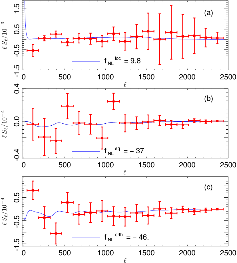
As mentioned before, our analysis went beyond the simple application of the KSW estimator to the SMICA map. All pipelines developed for Planck analysis were applied to all component-separated maps by SMICA, NILC, SEVEM, and C-R. We found from simulations in the previous Sections that the KSW, binned, and modal pipelines saturate the Cramér-Rao bound, while the wavelet estimator in its current implementation provides slightly suboptimal results. Wavelets remain however a useful cross-check of the other methods, also given some technical complementarities, e.g., they are the only approach that does not require inpainting, as explained in Sect. 3. Hence we include wavelet results, but only for SMICA. The results for the optimal KSW, binned and modal bispectrum estimators, for the four component separation methods, are summarized in Table 9, one of the main products of our analysis of Planck data. The wavelet bispectrum analysis of SMICA is reported in Table 10. In the analysis, the KSW and binned bispectrum estimators considered multipoles up to , while the modal estimator went to . As shown in Sect. 8.1 and Table 16, error bars and central values for the three primordial shapes have converged at , so the final primordial estimates from the three pipelines are directly comparable.121212The lower for the modal pipeline is also a conservative choice in view of the large survey of “non-standard” models that will be presented in Sect. 7.3
The binned bispectrum estimator used 51 bins, which were determined by optimizing the expected variance of the different parameters, focusing in particular on the primordial shapes.131313The boundary values of the bins are: 2, 4, 10, 18, 27, 39, 55, 75, 99, 130, 170, 224, 264, 321, 335, 390, 420, 450, 518, 560, 615, 644, 670, 700, 742, 800, 850, 909, 950, 979, 1005, 1050, 1110, 1150, 1200, 1230, 1260, 1303, 1346, 1400, 1460, 1510, 1550, 1610, 1665, 1725, 1795, 1871, 1955, 2091, 2240, and 2500 (i.e., the first bin is [2,3], the second [4,9], etc., while the last one is [2240,2500]). The modal estimator employed a polynomial basis () previously described in Fergusson et al. (2010a), but augmented with a local shape mode (approximating the SW large-angle local solution) to improve convergence in the squeezed limit. The above choices for the binned and modal methods produce a very high correlation (generally or better) of the expanded/binned templates with the exact ones used by the KSW estimator. The wavelet estimator is based on third-order statistics generated by the different possible combinations of the wavelet coefficient maps of the SMHW evaluated at certain angular scales. See for example Antoine & Vandergheynst (1998) and Martínez-González et al. (2002) for detailed information about this wavelet. We considered a set of 15 scales logarithmically spaced between 1.3 and 956.3 arcmin and we also included the unconvolved map. The wavelet map (Eq. (65)) for each angular scale has an associated extended mask generated from the mask U73 following the procedure described and extensively used in Curto et al. 2009b, a, 2011a, 2011b, 2012; Donzelli et al. 2012; Regan et al. 2013. The wavelet coefficient maps are later combined into the third-order moments (Eq. (64)), for a total 816 different statistics, and these statistics are used to constrain through a test.
The high level of agreement between results from the KSW, binned and modal estimators, and from all the component separation pipelines, is representative of the robustness of our results with respect to residual foreground contamination, and is fully consistent with our preliminary MC analysis shown in Sect. 6. The scatter with wavelets is a bit larger, but this was expected due to the suboptimality of the wavelet estimator and is also in agreement with our MC expectations from the tests. Therefore wavelets do provide another successful cross-check.
7.2 Bispectrum reconstruction
As previously explained (see Sect. 3), in addition to looking in specific bispectrum-space directions and extracting the single number for given shapes, the binned and modal pipelines have the capability to generate a smoothed (i.e., either coarse-grained in -space, or truncated at a given expansion eigenmode) reconstruction of the full bispectrum of the data. See also Planck Collaboration XXIII (2013).
7.2.1 Modal bispectrum reconstruction
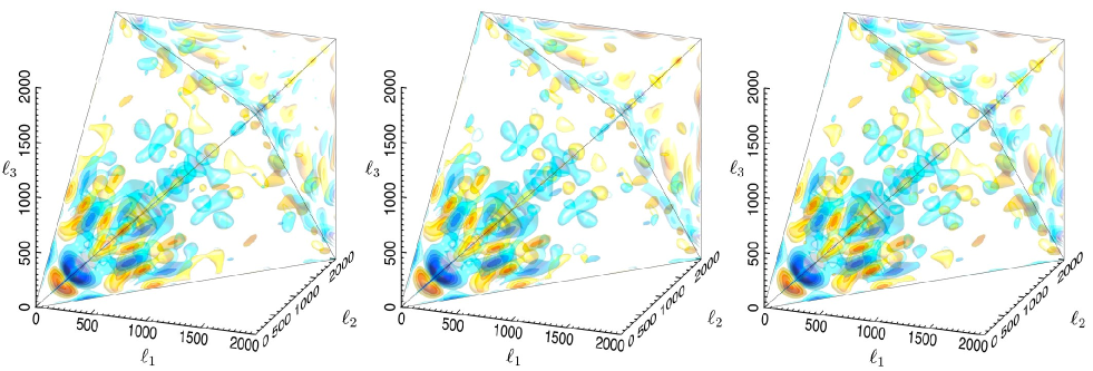
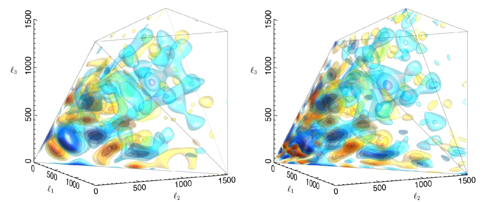
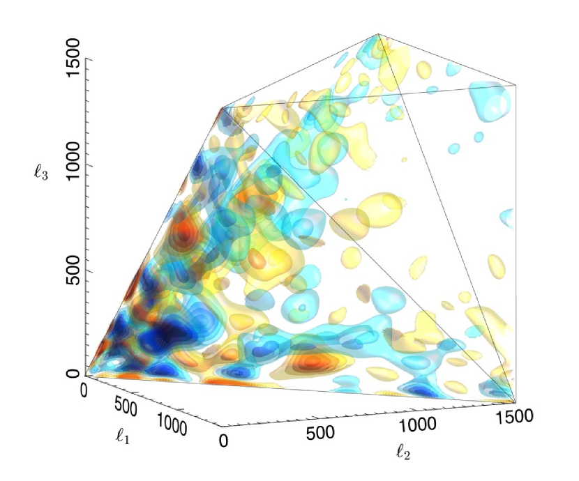
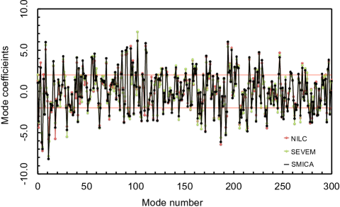
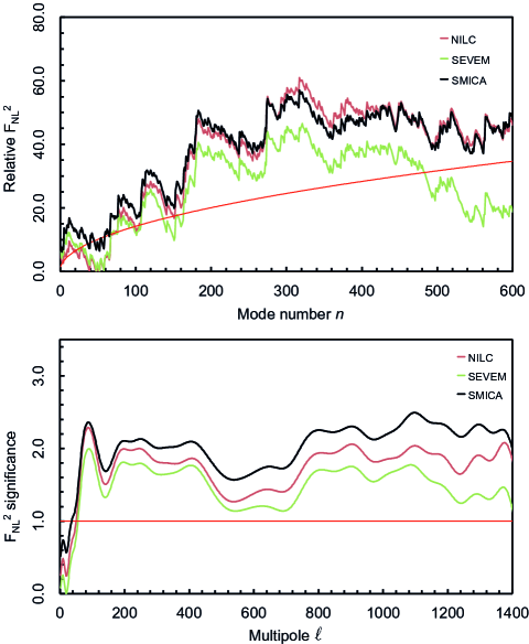
The modal pipeline was applied to the Planck temperature maps for the foreground-separation techniques SMICA, NILC, and SEVEM (Fergusson et al. 2010a). For this analysis we used two alternative sets of hybrid basis functions in order to cross-check results and identify particular signals. First, we employed trigonometric functions () augmented with the SW local mode, together with the three separable modes contributing to the CMB ISW-lensing signal. Secondly, we employed the same polynomial basis () with local SW mode as was used for estimation.
The modal coefficients extracted from the Planck SMICA, NILC, and SEVEM maps are shown in Fig. 9. Here we have used the hybrid Fourier modes with local and ISW-lensing modes. These amplitudes show remarkable consistency between the different maps, demonstrating that the alternative foreground separation techniques do not appear to be introducing spurious NG. Note that here the coefficients are for the orthonormalized modes (Eq. (69)) and they have a roughly constant variance, so anomalously large modes can be easily identified. It is evident, for example, that among the low modes there are large signals, which include the ISW-lensing signal and point source contributions.
Using the modal expansion of Eq. (50) with Eq. (69), we have reconstructed the full 3D Planck bispectrum. This is illustrated in Fig. 6, where we show “tetrapyd” comparisons between different foreground cleaned maps. The tetrapyd (see Fig. 1) is the region defined by the multipoles that obey the triangle condition, with . The 3D plots show the reduced bispectrum of the map, divided by a Sachs-Wolfe CMB bispectrum solution for a constant primordial shape, . This constant primordial bispectrum template normalizaton is carried out in order to remove an scaling from the starting bispectrum (it is analogous to multiplication of the power spectrum by ). To facilitate the interpretation of 3D bispectrum figures, note that squeezed configurations lie on the edges of the tetrapyd, flattened on the faces and equilateral in the interior, with on the diagonal. The colour levels are equally spaced with red denoting positive values, and blue denoting negative. Given the correspondence of the coefficients for SMICA, NILC, and SEVEM, the reconstructed 3D signals also appear remarkably consistent, showing similar contours out to . At large multipoles approaching , there is increased randomness in the reconstruction due to the rise in experimental noise and some evidence for a residual point source contribution.
There are some striking features evident in the 3D bispectrum reconstruction which appear in both Fourier and polynomial representations, as shown in more detail in Fig. 7. There is an apparent oscillation at low already seen in WMAP-7 (Fergusson et al. 2012). Beyond out to there are further distinct features (mostly “flattened” on the walls of the tetrapyd), and an oscillating ISW-lensing contribution can be discerned in the squeezed limit. For comparison, the bispectrum reconstruction for one of the lensed Gaussian simulations described in sec. 6.2 is shown in Fig. 8. ISW-lensing oscillating signatures in the squeezed limit are visible also in this case. When comparing results from a single simulation to the data, it is however always useful to keep in mind that the observed tetrapyd pattern is quite realization dependent, since full bispectrum reconstructions are noisy. Whatever its origin, Gaussian or otherwise, Fig. 7 reveals the CMB bispectrum of our Universe as observed by Planck.
The cumulative sum over the squared orthonormal coefficients from Eq. (70) for the Planck data is illustrated in Fig. 10 (upper panel). The Planck bispectrum contribution can be directly compared with Gaussian expectations averaged from 200 lensed Gaussian maps with simulated residual foregrounds. It is interesting to note that the integrated bispectrum signal fairly consistently exceeds the Gaussian mean by around over much of the domain. This includes the ISW and PS contributions for which subtraction only has a modest effect. Also shown (lower panel) is the corresponding cumulative quantity as a function of multipole , for which features have visible counterparts at comparable in Fig. 7. Despite the high bispectrum signal, this -test over the orthonormal mode coefficients is cumulatively consistent with Gaussianity for each of the three component separation methods considered. It is however important to stress that this is a model independent integrated measurement of NG. Fitting the data with specific bispectrum templates can of course enhance the signal-to-noise ratio for given models, especially in light of the to excess with respect to the Gaussian expectation, shown in the lower panel. This measurement is thus not in disagreement with detection of a residual point source (Poisson) bispectrum in the same maps (see Table 3), or with the results shown in our feature models survey of Section 7.3.3. We also note some differences in the high mode region between SEVEM and the other two methods, with the SEVEM results being closer to the Gaussian expectation. This is consistent with tests on simulations and with SEVEM measuring a slightly lower ISW-lensing amplitude than the other methods (see Table 2). On the other hand the discrepancies are well within statistical bounds, as it can be seen by comparing them to the Gaussian standard deviation from simulations (red line). We thus conclude that, even accounting for these high modes deviations, the different component separation methods display a good level of internal consistency. It is also important to notice that this already good level of agreement becomes even stronger in “non-blind” measurements, when primordial bispectrum templates are fit to the data, and specific theoretically relevant regions of the tetrapyd are selected. This can be clearly seen from Table 9.
7.2.2 Binned bispectrum reconstruction
As explained in Sect. 3.4.2, it is interesting to study the smoothed observed bispectrum divided by its expected standard deviation, since this will indicate if there is a significant deviation from Gaussianity for certain regions of -space. This quantity is shown in Figs. 11 and 12 as a function of and , for two different values (or rather, bins) of : the intermediate value [610,654] in Fig. 11 and the high value [1330,1374] in Fig. 12. Each figure shows the results for the SMICA, NILC, SEVEM, and C-R cleaned maps as well as for the raw 143 GHz channel map. For comparison, the result for one of the lensed Gaussian simulations described in Sect. 6.2 is also shown. The bispectra were obtained with the binned bispectrum estimator and smoothed with a Gaussian kernel as explained in Sect. 3.4.2. Very blue or red regions indicate significant NG, regions that are less red or blue just represent expected fluctuations of a Gaussian distribution.
From Fig. 11 at an intermediate value of we can conclude that there is a very good agreement between SMICA, NILC, and SEVEM for all values of and , and with C-R up to about . In fact, up to there is also a good agreement with the raw 143 GHz channel. We also see no significant non-Gaussian features in this figure (except maybe in the C-R and raw maps at ). The lensed Gaussian simulation in the last panel looks quite Gaussian as well (as it should), but very different from the others. This is not surprising, as all we are seeing here are the small random fluctuations that exist in any Gaussian realization, and the simulation represents of course another realization than the real data. (Note that the ISW-lensing NG, while present in the simulation, is not really visible in the particular slices shown here due to the linear scale of the axes and the fact that the ISW-lensing NG peaks in the squeezed configuration.)
Figure 12 at a high value of , on the contrary, shows significant non-Gaussian features in the raw map, but much less NG in the cleaned maps. In particular one can see the point-source bispectral signal at high- approximately at equilateral configurations in the data. This is absent in the the lensed Gaussian simulation, which has no point sources. There is still an excellent agreement between SMICA, NILC, and SEVEM. The C-R map shows less NG than the other three cleaned maps, which is consistent with the absence of a detection of the Poisson point source bispectrum for C-R, see Table 3.
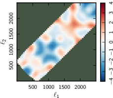
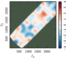
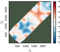
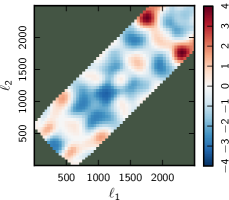
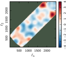
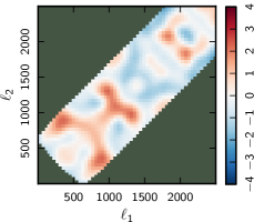
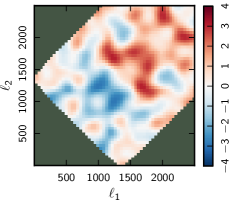
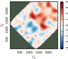
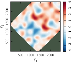
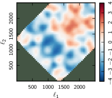
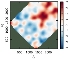
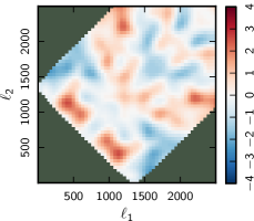
7.3 Constraints on specific targeted shapes
We have deployed the modal estimator to investigate a wide range of the inflationary models described in Sect. 2. This is the same validated estimator for which the standard results have been reported in the Sect. 7, but it is augmented with the primordial modal decomposition and projection described in Sect. 3.2.3. The resulting modal-projected local, equilateral and orthogonal shapes are 99% correlated with those found using direct integration of Eq. (42) (as for the analysis above). Modal correlations for the other models investigated were determined for both the primordial shapes and the late-time projected decompositions and were all above 90%, unless stated otherwise. This primordial modal estimator pipeline has been applied already extensively to the WMAP-7 data (Fergusson et al. 2012).
7.3.1 Nonseparable single-field bispectrum shape results
Having characterised single-field inflation bispectra using combinations of the separable equilateral and orthogonal ansätze, we note that the actual leading-order non-separable contributions (Eqs. (6, 2.1)) exhibit significant differences in the collinear (flattened) limit. For this reason we provide constraints on DBI inflation (Eq. (2.1)) and the two effective field theory shapes (Eqs. (2.1, 6)), as well as the ghost inflation bispectrum, which is an exemplar of higher-order derivative theories (specifically Eq. (3.8) in Arkani-Hamed et al. 2004). Using the primordial modal estimator, with the SMICA foreground-cleaned data, we find:
| (92) |
where we have normalized with the usual primordial convention which is shape-dependent (i.e., the central value of the shape function is taken such that ). In parentheses we also give a reweighted constraint for easier comparison with the equilateral constraint from the same modal estimator, i.e., we have rescaled using the Fisher variance for the closely-related equilateral shape. Given the strong cross-correlation (above 95%) between all these models, the equilateral family results of (7.3.1) reveal larger differences around than might be expected (and somewhat larger than observed previously in the WMAP data (Fergusson et al. 2012)). The reason for this variation between the equilateral shapes in Planck appears to be the additional signal observed in the flattened limit in the bispectrum reconstruction beyond the WMAP signal-dominated range (see Fig. 6). There is also a contribution from the small correlation difference between equilateral models from primordial modal and KSW methods. The results for these models for all the SMICA, NILC and SEVEM foreground-separated maps are given in Appendix C (Table 24).
|
7.3.2 Non-Bunch-Davies vacuum results
We have investigated the non-separable shapes arising from excited initial states (non-Bunch-Davies vacuum models) which usually peak in the flattened or collinear limit. In particular, we have searched for the four non-separable bispectra described in Eqs. (14) and (15), as well as the original flattened shape (Eq. (6.2-3) in Chen et al. 2007b). This entails choosing suitable cut-offs to ensure that the signal is strongly flattened (i.e., distinct from flat in Eq. (13)), while also accurately represented by the modal expansion at both early and late times (Eqs. (59, 60)). For , we adopted the same edge truncation and mild Gaussian filter described in Fergusson et al. (2012), while for and , which are described by Eq. (14), we chose , and in Eq. (15) we take . The shape correlations for most non-Bunch-Davies vacua were good (above 90%), except for the strongly squeezed model with oscillations of Eq. (14) which was relatively poor (60%). Together with the orthogonal (Eq. (4)), flat (Eq. (13)) and vector (Eq. (19)) shapes, these non-Bunch-Davies models explore a broad range of flattened models, with a variety of different widths for picking out signals around the faces of the tetrapyd (see Fig. 1).
The results obtained for the non-Bunch-Davies models from the different foreground-cleaned map bispectra were consistent and the constraints from SMICA (for brevity) are given in Table 11. More comprehensive results from SMICA, NILC and SEVEM can be found in Table 24 in Appendix C. Both and (Eq. (14)) produced raw results above , in part picking out the flattened signal observed in the bispectrum reconstruction in Fig. 6. However, these flattened squeezed signals are also correlated with CMB ISW-lensing and so, after subtracting the predicted ISW bias (as well as the measured point source signal), most NBD results were reduced to or less (see “Clean ” column in Table 11). The exception was the most flattened model which remained higher , i.e., with signals at , and for SMICA, NILC and SEVEM respectively.
We emphasise that this has to be considered just as preliminary study of flattened NG in the Planck data using four exemplar models. In order to reach a complete statistical assessment of constraints regarding flattened models in forthcoming analyses, we will have to undertake a systematic search for best-fit Planck NBD models using the parameter freedom available.
7.3.3 Scale-dependent feature and resonant model results
We have investigated whether the Planck bispectrum reconstructions include oscillations expected in feature or resonant models (Eqs. (16, 17)). Although poorly correlated with scale-invariant shapes, the feature and resonant models have (at least) two free parameters - the period and the phase - forming a model space which must be scanned to determine if there is any significant correlation (in the absence of any physical motivation for restricting attention to specific periodicities). We have undertaken an initial survey of these models with the wavelength range defined by the native resolution of the present modal estimator (hybrid local polynomials with 600 modes), similar to the feature model search in WMAP data in Fergusson et al. (2012). For feature models of Eq. (16) we can obtain high correlations (above 95%) for the predicted CMB bispectrum if we take , that is, for an effective multipole periodicity feature models are accurately represented.
|
|||||||||||||||||||||||||||||||||||||||||||||||||||||||||||||||||||||||||||||
The results of a first survey of feature models in the Planck data is shown in Table 12 for and phases (for we will identify a correlation with the opposite sign). Again, there was good consistency between the different foreground-separation methods SMICA, NILC and SEVEM showing that the results are robust to potential residual foreground contamination in the data. For brevity we only give SMICA results here, while providing measurements from other component separation methods in Appendix C. Feature signals are typically largely uncorrelated with the ISW-lensing or point sources, but nevertheless we subtract these signals and give results for the cleaned . The Table 12 results show that there is a parameter region around for which signals well in excess of are possible (we undertook a broader search with but found only a low signal beyond ). It appears that some feature models are able to match the low- ‘plus-minus’ and other features in the Planck bispectrum reconstruction (see Fig. 6). The best fit model has () and phase with a signal . As a further validation step of our results, we also re-analysed the models with significance using a different modal decomposition, namely an oscillating Fourier basis () augmented with a local SW mode (the same used for the reconstruction plots in Sect. 7). The results from this basis are shown in Appendix C and they are fully consistent with the polynomial measurements presented here. The previous best-fit WMAP feature model, () and phase , attained a 2.15 signal with (Fergusson et al. 2012), but it only remains at this level for Planck.
We note however that the apparently high statistical significance of these results is much lower if we consider this to be a blind survey of feature models, because we are seeking several uncorrelated models simultaneously. Following what we did for our study of impact of foregrounds in Sect. 8, we considered a set of realistic lensed FFP6 simulations, processed through the SMICA pipeline, and including realistic foreground residuals. If we use this accurate MC sample to search for the same grid of 52 feature models as in Table 12, we find a typical maximum signal of . Searching across all feature models (see below) studied here yields an expected maximum (whereas the survey for all 511 models from all paradigms investigated yielded ). This means that our best-fit model from data has a statistical significance below above the maximum signal expectation from simulations, so we conclude that we have no significant detection of feature models from Planck data.
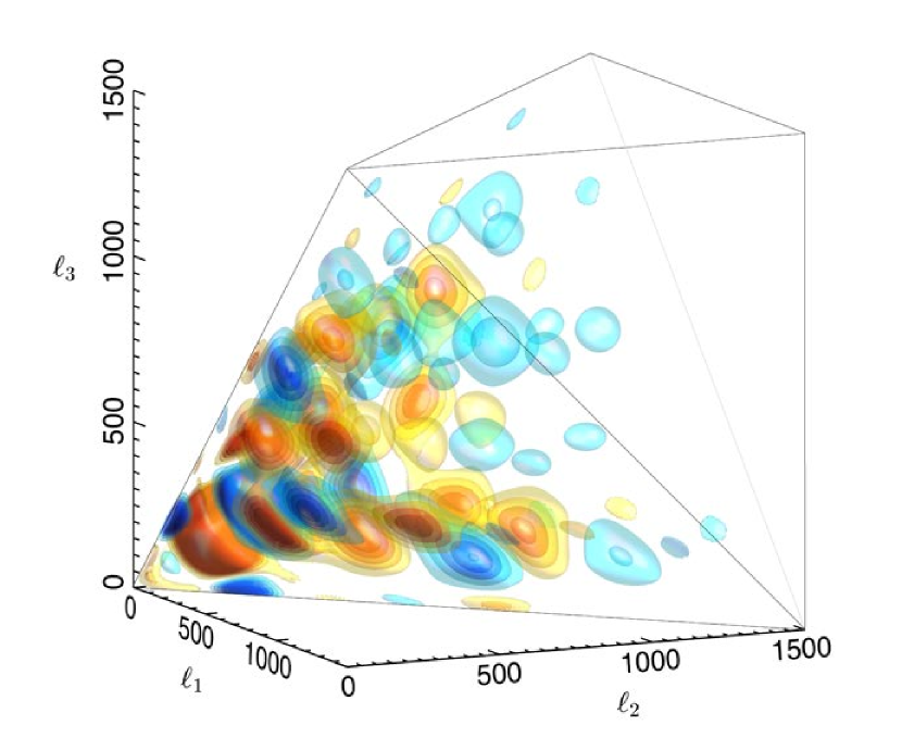
|
||||||||||||||||||||||||||||||||||||||||||
Feature models typically have a damping envelope representing the decay of the oscillations as the inflaton returns to its background slow-roll evolution. Indeed, the feature envelope is a characteristic of the primordial mechanism producing the fluctuations, decaying as increases for inflation while rising for contracting models like the ekpyrotic case (Chen 2011). We have made an initial survey to determine whether a decaying envelope improves the significance of any feature models. The envelope employed was a Gaussian centred at with a falloff and results for specific parameters are given in Table 13. The best fit model remains () with phase and the significance rises to , together with a second model () . However the caveats about blind survey statistics previously noted also do not allow a claim of any detection in this case. A plot of the best-fit feature model with a decay envelope is shown in Fig. 13, for which the main features should be compared with those in Fig. 7. Non-Gaussian bispectrum signals from feature models typically produce counterparts in the power spectrum as will be described in Sect. 9. An improved statistical interpretation of the results presented in this Section will be possible when this additional investigation will be completed.
We have also undertaken a survey of resonant models and the non-Bunch-Davies resonant models (or enfolded resonance models). With the modal estimator, we can achieve high accuracy for the predicted bispectrum for (note that this has a different logarithmic dependence to feature models and a varying effective ). For the resonance model shape of Eq. (2.3), we have not undertaken an extensive survey, except selecting a likely range for a high signal with periodicity comparable to the feature model, that is, with and phases . However, no significant signal was found (all below 1), as can be verified in Table 22 in Appendix C. For the enfolded resonance model shape of Eq. (2.3) , we have undertaken a preliminary search in the range with the same phases. Again, no significant signal emerges from the Planck data, as shown in Table 23 in Appendix C.
7.3.4 Directional dependence motivated by gauge fields
We have investigated whether there is significant NG from bispectrum shapes with non-trivial directional dependence (Eq. (19)), which are motivated by inflationary models with vector fields. Using the primordial modal estimator we obtained a good correlation with the flattened-type model, but the squeezed model produced a relatively poor correlation of only 60%, given the complexity of the dominant squeezed limit. Preliminary constraints on these models are given in the Table 11, showing no evidence of a significant signal.
7.3.5 Warm inflation
Warm inflation produces a related shape with a sign change in the squeezed limit. This also had a poor correlation, until smoothing (WarmS) was applied as described in Fergusson et al. (2012). The resulting bispectrum shows no evidence for significant correlation with Planck data (SMICA),
| (93) |
The full list of constraints for SMICA, NILC and SEVEM models can be found for warm inflation and vector models in Table 24 in Appendix C.
7.3.6 Quasi-single-field inflation
Finally, quasi-single-field inflation has been analysed constraining the bispectrum shape of Q (Eq. (12)), that depends on two parameters, and . In order to constrain this model we have calculated modal coefficients for in steps of (so 151 models in total). These were then applied to the data and the one with the greatest significance was selected. Results are shown in Fig. 26. The maximum signal occurred at , . To obtain error curves we performed a full likelihood using 2 billion simulations following the method described in Sefusatti et al. (2012). Such a large number of simulations was possible as they were generated from the modal -covariance matrix which is calculated once from the 200 Planck realistic CMB simulations, rather than repeatedly from the CMB simulations themselves. The procedure is to take the correlation matrix for the models (this is just the normalized dot product of the modal coefficients). This is then diagonalised using PCA, after which only the first 5 eigenvalues are kept as the remaining eigenvalues are . The -covariance matrix is projected into the same sub-basis where it is also diagonalised via PCA into 5 orthonormal modes, with the two leading modes closely correlated with local and equilateral. The procedure by which to produce a simulation is to generate five Gaussian random numbers and add the mean values obtained from the Planck data, rotating them to the sub-basis where we determine the with the greatest significance. The result is then projected back to the original space to determine the related . The two billion results from this MC analysis are then converted into confidence curves plotted in Fig. 26. The curve shows that there is no preferred value for with all values allowed at . This reflects the results obtained from data previously, where we found the least preferred value of had only a marginally lower significance of (Sefusatti et al. 2012). Of course, these conclusions are directly related to the null results for both local and equilateral templates.
7.4 Constraints on local non-Gaussianity with Minkowski Functionals
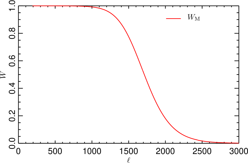
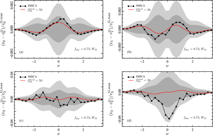
| Setup (MFs) Gaussian ideal 0.2 10.7 Realistic noise, 12 13 Mask (), realistic noise 12 18 |
| Map . Source Corresponding Raw map . 19.1 19.3 Lensing subtracted . 8.5 20.5 Lensing 10.6 Lensing+PS subtracted . 7.7 20.3 Point sources 0.8 Lensing+CIB subtracted . 7.5 20.5 CIB 1.0 Lensing+SZ subtracted . 6.0 20.4 SZ 2.5 All subtracted . 4.2 20.5 All 14.9 |
In this Subsection, we present constraints on local NG obtained with Minkowski Functionals (MFs). MFs describe the morphological properties of the CMB field and can be used as generic estimators of NG (Komatsu et al. 2003; Eriksen et al. 2004; De Troia et al. 2007; Hikage et al. 2008; Curto et al. 2008; Natoli et al. 2010; Hikage & Matsubara 2012; Modest et al. 2013). As they are sensitive to every order of NG, they can be used to constrain different bispectrum and trispectrum shapes (Hikage et al. 2006, 2008; Hikage & Matsubara 2012). They are therefore complementary to, and a useful validation of, optimal estimators. Their precise definition and analytic formulations are presented in Planck Collaboration XXIII (2013). The MF technique is also used in the companion paper Planck Collaboration XXV (2013).
We review here the properties of MFs, as a complementary tool to poly-spectrum based estimators.
First, they are defined in real space, which makes MFs robust to masking effects and no linear term is needed to take into account the anisotropy of the data model. Second, as MFs are sensitive to every non-Gaussian feature in the maps, they can be a useful probe of every potential bias in the bispectrum measurement, in particular the different astrophysical contaminations (foregrounds and secondaries).
There is a limitation to MF studies: they can be expressed in terms of weighted sums of the bispectrum (and trispectrum) in harmonic space (Matsubara 2010), hence the angle-dependence of the bispectrum is partially lost. This makes MFs suboptimal in two ways: increasing error bars for constraints on specific shapes and reducing the distinguishability of different bispectrum shapes. This lack of specificity can introduce biases, as MFs will partially confuse primordial and non-primordial sources of NG and can introduce degeneracies between different primordial shapes. Constraints on orthogonal and equilateral shapes are quite degenerate with MFs, we therefore chose here to focus on the local bispectrum shape. We also leave trispectrum analyses for future studies.
An attractive feature of MFs is their linearity for weak NG () and weak signals (such as point sources, and Galactic residuals after masking and component separation) (Ducout et al. 2013). This property can be used to estimate different known non-primordial contributions.
7.4.1 Method
We constrain using the optimized procedure described in Ducout et al. (2013). To obtain constraints on , we apply a specific Wiener filter on the map (), shown in Fig. 14. We do not use here the filter designed to enhance the information from the gradients of the map (), because this filter is very sensitive to small-scale effects and may be biased by foreground residuals.
We use maps at HEALPix resolution (Górski et al. 2005) and . Our results are based on the four normalized141414Raw MFs depend on the Gaussian part of fields through a normalization factor that is a function only of the power spectrum shape. We therefore normalize functionals to focus on NG; see Planck Collaboration XXIII (2013) and references therein. functionals (respectively Area, Perimeter, Genus and ), computed on thresholds , between and in units of the standard deviation of the map.
We combine all functionals into one vector (of size ). We then analyse this vector in a Bayesian way to obtain a posterior for the , and hence an estimate of this parameter. The principle is to compare the vector measured on the data to the ones measured on non-Gaussian simulations with the same systematic effects (realistic noise, effective beam) and data processing (Wiener filtering) as the data, . Modelling the MFs as multivariate Gaussians we obtain the posterior distribution for with a test :
| (94) |
with
| (95) |
Since NG is weak, the covariance matrix is computed with Gaussian simulations, again reproducing effective beam, realistic noise and filtering of the data. The dependence of the MFs on , , is obtained as an average of measured on 100 simulations. The simulations used here are based on the WMAP-7 best-fit power spectrum (Komatsu et al. 2011), using the procedure described in Elsner & Wandelt (2009).
7.4.2 Validation tests
We report here validation of the MFs estimator on in thoroughly realistic Planck simulations. This validation subsection is analogous to Sect. 6.1 concerning bispectrum-based estimators. The same tests (ideal Gaussian maps, full-sky non-Gaussian maps with noise and non-Gaussian maps with noise and mask) are performed, but different non-Gaussian simulations are used. Non-Gaussian CMB simulations as processed in Fergusson et al. (2010a) only guarantee the correctness of the 3-point correlations. Since the MFs are sensitive to higher-order -point functions, they were validated with physical simulations (Elsner & Wandelt 2009).
The first test consists of 100 simulations of a full-sky Gaussian CMB, with a Gaussian beam with FWHM of 5 arcmin and without any noise, cut off at , with . Here validation tests were made at , but results (estimate and error bars) remain the same at as we keep the same . The second test includes non-Gaussian simulations with and realistic coloured and anisotropic noise, processed through the Planck simulation pipeline and the component-separation method SMICA. Finally, in the third test we add the union mask U73 to the previous simulations, masking both the Galaxy and the brightest point sources, and leaving of the sky unmasked. Only the inpainting of the smallest holes in the point sources part of the mask was performed. For these three tests, the results are presented in Table 14. We give here the average estimate and error bar obtained on the 100 simulations, when we use the four functionals. The results show that the MF estimator is unbiased, robust, and a competitive alternative to bispectrum-based estimators. Moreover a map-by-map comparison of the results obtained on with KSW and MFs estimators showed a fair agreement between the two methods.
7.4.3 Results
For our analysis we considered a foreground-cleaned map obtained with the component separation method SMICA at and . As for the previous results in this Section, we used the union mask U73, which leaves % of the sky after masking Galaxy and point sources. To take into account some instrumental effects (asymmetry of beams, component separation processing) and known non-Gaussian contributions (lensing), we used realistic unlensed and lensed simulations () of Planck data (FFP6 simulations, see Appendix A). First, MFs were applied to the unlensed simulations and the resulting curves served to calibrate the estimator, as the Gaussian part of the NG curves 151515The overall effect of data processing on the constraint from MFs was evaluated as .. This estimate is referred to as the “raw map”. Secondly, MFs were applied to the lensed simulations, and the same procedure was applied, the result being referred as “lensing-subtracted”. We summarize the procedure in the following equation:
| (96) |
Here we assume that the MF respond linearly to lensing at first order and that primordial NG and lensing contributions are therefore additive.
Additionally, we tried to characterize other non-primordial contributions that one could expect in masked SMICA-cleaned maps covering % of the sky. To this end, we used simulations of extragalactic foregrounds and secondary anisotropies: uncorrelated (Poissonian) point sources; clustered CIB; and SZ clusters. These component simulations reproduce accurately the whole Planck data processing pipeline (beam asymmetry, component separation method). Using the linearity of MFs (Ducout et al. 2013), we could introduce these effects as a simple additive bias on the curves following
| (97) |
where is the average bias measured on 100 simulations. Note that the SZ simulation does not take into account the SZ-lensing correlation, which is expected to be negligible given the error bars.
Results are summarized in Table 15 and MFs curves are shown in Fig. 15, without including the lensing subtraction (“raw curves”). Considering the larger error bars of MF estimators, the constraints obtained are consistent with those from the bispectrum-based estimators, even without subtracting the expected non-primordial contributions. Moreover, results are quite robust to Galactic residuals: constraints obtained with other component separation methods (NILC and SEVEM), with different sky coverage, differ from the SMICA results presented here by less than .
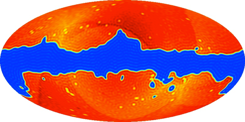
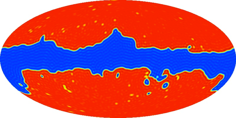
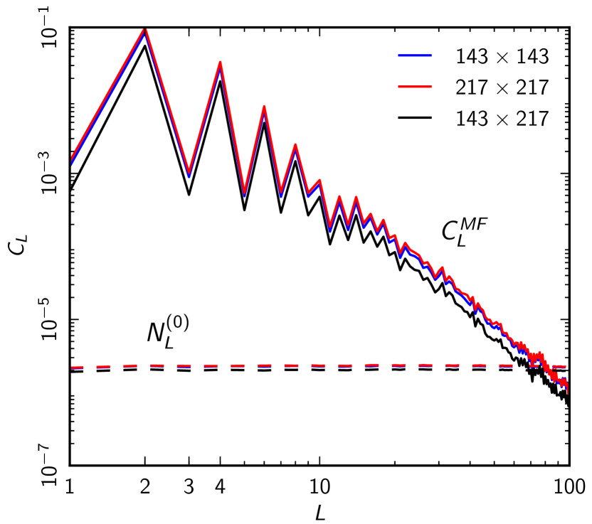
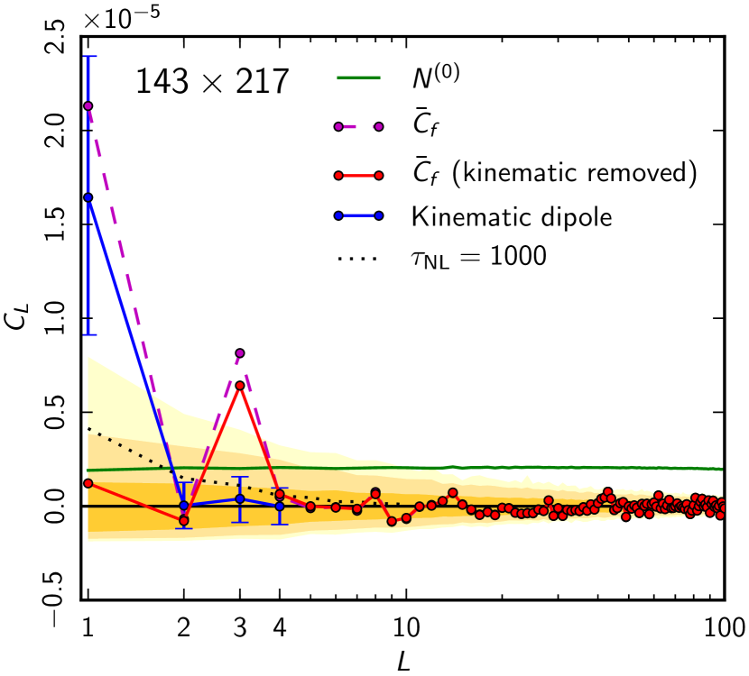
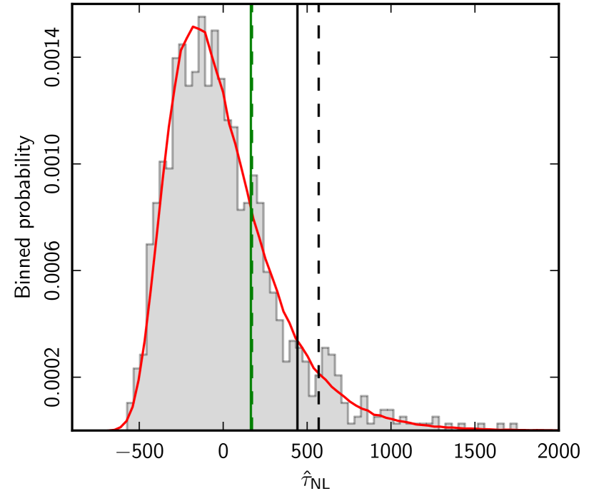
7.5 CMB trispectrum results
As shown in Fig. 16 the modulation reconstruction mean field has two large contributions, one from the mask and one from anisotropic noise, reflecting the fact that they both look like a large spatially-varying modulation of the fluctuation power. The noise we use to estimate the mean field is taken from FFP6 simulations, adjusted with an additional white noise component to match the power spectrum in the observed maps. However this is still only an approximate description of the instrumental noise present in the data. The mean field from non-independent maps (e.g., GHz maps) shows a large noise anisotropy that is primarily quadrupolar before masking, and any mismatch between the simulated noise and reality would lead to a large error in the mean field subtraction. By instead using the modulation estimator for GHz maps errors due to misestimation of the noise are avoided, and the mean field is then dominated by the shape of the Galactic cut, which is well known, and a smaller uncertainty from assumed simulation power spectrum and beam errors (see Fig. 16). For this reason for our main result we work with modulation reconstructions generated from GHz maps with independent noise, which removes the leading error due to noise mean field misestimation.
Figure 17 shows the reconstructed modulation power from GHz maps that we use for our analysis. We show two results: one where we do not include the expected kinematic dipole signal in the mean field subtraction (see Sect. 5.4), and one were we do so that the reconstruction should then be dominated by the primordial and any unmodelled systematic effects. In the first case the result gives a clear first detection of the dipolar kinematic modulation signal of roughly the expected magnitude (see Planck Collaboration XXVII (2013) for a more detailed discussion of this signal). Including the expected kinematic signal in the simulations (and hence the mean field) removes this signal, giving a cosmological modulation reconstruction that is broadly consistent with no modulation (statistical isotropy) except for the anomalous very significant signal in the modulation octopole.
Note that only the two-point reconstruction is free from noise bias, the four-point is still sensitive to noise modelling at the level of the subtraction of the reconstruction noise power spectrum (Eq. (78)). However as shown in the Fig. 17, is not that much larger than the reconstruction scatter at low multipoles where the signal peaks, so the sensitivity to noise misestimation is much less than in the mean field subtraction (where the large-scale noise anisotropy gives a large-scale mean field in the auto-estimators orders of magnitude larger, Fig. 16).
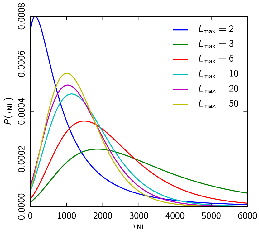
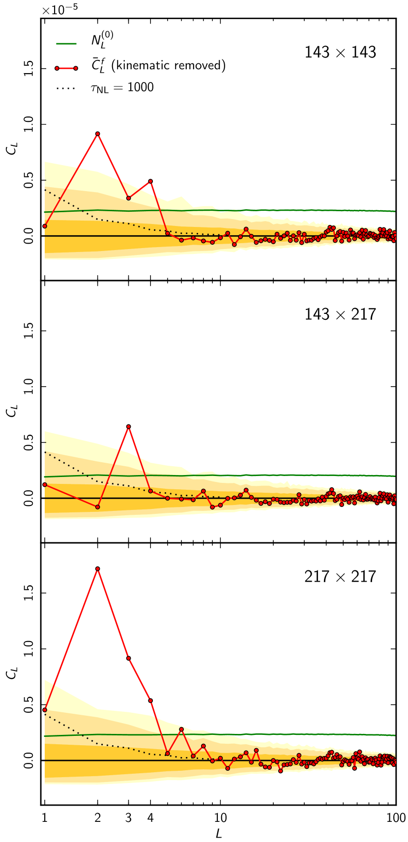
The estimator from the GHz modulation reconstruction gives , compared to a null hypothesis distribution at CL (). Our quoted error bar is assuming zero signal so that there is no signal cosmic variance contribution, and the bulk of the apparent signal is coming from the high octopole seen in Fig. 17. The alternative estimator gives a slightly different weighting to the octopole, giving with an expected null-hypothesis . The surprisingly large difference between the estimators can be explained as due to the large octopole signal, which has . However the shape of the total signal would not be expected from a genuine signal, since as shown in Fig. 17 on average the latter is expected to fall off approximately proportional to (i.e., a large primordial would be expected in most realisations to give large dipole and quadrupole signals that we do not see). If we estimate using we obtain with only a slightly larger null-hypothesis error , where in this case .
Note that the distribution of is quite skewed because the signal is dominated by the very-low multipole modulation power spectra which have skewed -like distributions due to the large cosmic variance there (see Fig. 18; Hanson & Lewis 2009; Smith & Kamionkowski 2012). The reconstruction noise acts like nearly-uncorrelated Gaussian white noise, so each of the comes from a sum of squares of modulation reconstruction modes; the shape of the distribution is consistent with what would come from calculating a weighted sum of -distributed random variables. If we assume that any primordial modulation modes giving rise to a physical signal are also Gaussian, for any given physical the estimators would also have distributions. This allows us to evaluate the posterior distribution of given the observed , in exactly the same way that one can do for the CMB temperature power spectrum. For each the posterior distribution on the full sky would have an inverse-gamma distribution. We follow Hamimeche & Lewis (2008) by generalizing this to a cut-sky approximation for a range of multipoles:
| (98) |
where is the covariance of the estimators calculated from null hypothesis simulations, is the estimator reconstruction noise,
| (99) |
and
| (100) |
For uncorrelated -distributed estimators this distribution reduces to the exact distribution, a product of inverse-gamma distributions. This approximation to the posterior can be used to evaluate the probability of any scale dependent , and does not rely on compression into a single estimator; it can therefore fully account for the observed distribution of modulation power between . Here we focus on the main case of interest where is nearly-scale-invariant so that for all we have .
The resulting posterior distributions of are shown in Fig. 19 for a range of . These are strongly skewed, in the same way as the posterior from the low quadrupole in the CMB temperature data. The high octopole is pulling the distributions up to higher values, but increasing can reduce the high- tail because very large values are inconsistent with the low modulation power seen at . With the posterior peaks near zero, but the distribution is then very broad because there are only about 8 modes, which therefore have large cosmic variance. For we find at CL, which we take as our upper limit.
Figure 20 shows the modulation reconstructions for the 143 GHz and 217 GHz maps separately compared to the cross estimator. The picture is complicated here by the large signals from noise misestimation seen in the and estimators, however the fact that the octopole in is lower than in the cross-estimator indicates that the octopole signal is very unlikely to be mainly physical. Our measured limit in practice represents a strong upper limit on the level of primordial that could be present, since unmodelled varying small-scale foreground or non-constant gain/calibration would also only serve to increase the measured estimate compared to primordial on average. The octopole signal does vary slightly with Galactic mask, though at present we cannot clearly isolate its origin. If more extensive analysis (for example using cross-map estimators at the same frequency) can identify a non-physical origin and remove it, the quoted upper limit on would become significantly tighter. For a more extensive discussion of possible foreground and systematic effect issues that can affect 4-point estimators see Planck Collaboration XXVII (2013); Planck Collaboration XVII (2013).
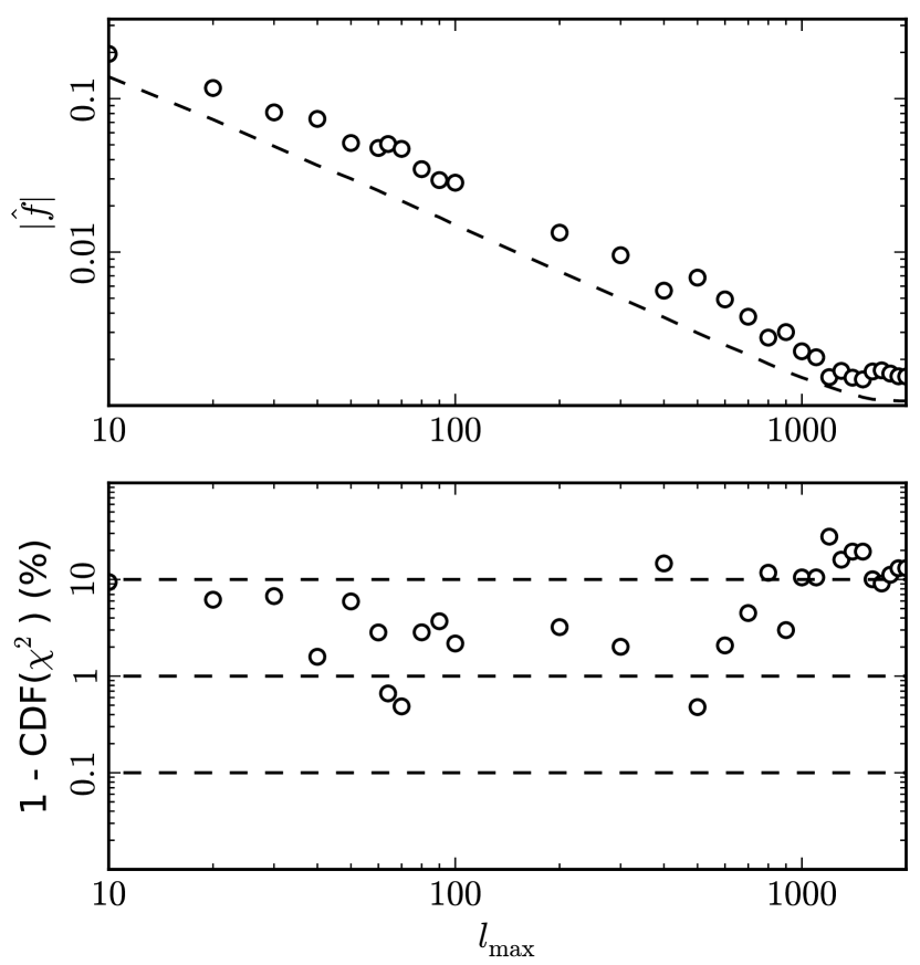
We have focussed on nearly scale invariant modulations here. As discussed in Planck Collaboration XXIII (2013) there are some potentially interesting “anomalies” in the distribution of power in the Planck data, especially the hemispherical power asymmetry at . If these power asymmetries are physical rather than statistical flukes, they must be strongly scale-dependent, and would correspond to a scale-dependent -like trispectrum. As we have shown here the dipole power asymmetry does not persist to small scales, except for the signal aligned with the CMB dipole expected from kinematic effects: from our analysis using we find a primordial consistent with Gaussian simulations, corresponding to a dipole modulation amplitude . To be consistent with a modulation at and modulation at , as seen in the lower- anisotropies of both WMAP and Planck the primordial trispectrum would have to be strongly scale-dependent on small-scale modes, so that larger small-scale modes are modulated more than the smallest ones (rather than just ). Fig. 21 shows how the allowed dipole modulation amplitude drops as increases (similar to Fig. 3 of Hanson & Lewis (2009) for WMAP, but now extending to the higher available from Planck). This result is consistent with Planck Collaboration XXIII (2013), where different estimators and analysis cuts also find no evidence of primordial dipole-like power asymmetry on small scales, but confirm the large-scale distribution of power seen with WMAP and also a marginally-significant smaller-amplitude () dipole-like modulation at .
8 Validation of Planck results
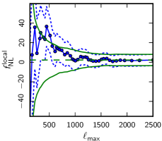
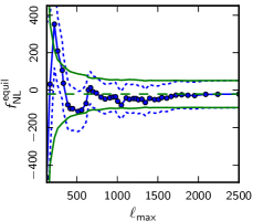
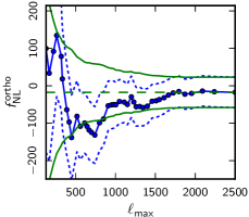
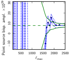
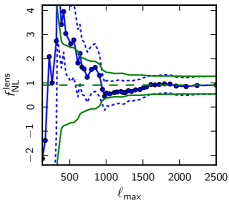
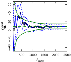
| Shape . KSW Local . 38 18 6.4 9.7 6.9 6.2 9.1 5.8 9.8 5.8 Equilateral . 119 121 45 88 41 75 40 75 37 75 Orthogonal . 163 109 89 52 57 45 45 40 46 39 Diff.ps . (1.5 1.3) (7.9 3.1) 39 18 10.0 3.1 7.7 1.5 ISW-lensing . 3.2 1.2 1.00 0.43 1.00 0.35 0.83 0.31 0.81 0.31 Binned Local . 33 18 6.6 9.8 7.1 6.1 8.5 5.9 9.2 5.9 Equilateral . 95 107 55 77 47 72 22 73 20 73 Orthogonal . 102 94 69 58 60 44 35 40 39 41 Diff.ps . (1.4 1.2) (8.2 2.9) 42 17 9.9 2.9 7.7 1.6 ISW-lensing . 2.6 1.6 0.57 0.52 0.80 0.42 0.85 0.38 0.91 0.37 |
Here we perform a set of tests to check the robustness and stability of our measurements. As these are validation tests of Planck results, and not internal comparisons of bispectrum pipelines (already shown to be in tight agreement in Sect. 6 and 7) we will not employ all the bispectrum estimators on each test. In general we choose to use two estimators on each test, in order to have a cross-check of the outcomes without excessive redundancy.
|
||||||||||||||||||||||||||||||||||||||||||||||||||||||||||||||||||||||||
8.1 Dependence on maximum multipole number
The dependence on the maximum multipole number of the SMICA results (assuming independent shapes) is shown in Fig. 22 (for the binned estimator) and Table 16 (for both the KSW and binned estimators). Testing the dependence is easiest for the binned estimator, where one can simply omit the highest bins in the final sum when computing . It is clear that we have reached convergence both for the values of and for their error bars at , with the possible exception of the error bars of the diffuse point-source bispectrum. The diffuse point-source bispectrum template is dominated by equilateral configurations at high . Moreover, for all the shapes except point sources, results at are very close to those at , taking into account the size of the error bars.
It is very interesting to see that at we find a local result in very good agreement with the WMAP-9 value of (Bennett et al. 2012) (or after ISW-lensing bias subtraction). At these low values we also find negative values for orthogonal , although not as large or significant as the WMAP-9 value (which is ). One can clearly see the importance of the higher resolution of Planck both for the values of the different parameters and for their error bars.
It is also clear that the higher resolution of Planck is absolutely crucial for the ISW-lensing bispectrum; this is simply undetectable at WMAP resolution. On the other hand, the high sensitivity of Planck measurements also exposes us to a larger number of potentially spurious effects. For example we see that the bispectrum of point sources is also detected at high significance by Planck at , while remaining undetectable at lower resolutions. The presence of this bipectrum in the data could in principle contaminate our primordial measurements. For this reason, the presence of a large point source signal has been accounted for in previous Sections by always including the Poisson bispectrum in a joint fit with primordial shapes. Fortunately, it turns out that the very low correlation between the primordial templates and the Poisson one makes the latter a negligible contaminant for , even when the residual point source amplitude is large.
8.2 Dependence on mask and consistency between frequency channels
|
||||||||||||||||||||||||||||||||||||||||||||||||||||||||||||||||||||||||||||||||||||||
To test the dependence on the mask, we have analysed the SMICA maps applying four different masks. Firstly the union mask U73 used for the final results in Sect. 7, which leaves 73% of the sky unmasked. Secondly we used the confidence mask CS-SMICA89 of the SMICA technique, which leaves 89% of the sky. Next, a bigger mask constructed by multiplying the union mask U73 with the Planck Galactic mask CG60, leading to a mask that leaves 56% of the sky. And finally a very large mask, leaving only 32% of the sky, which is the union of the mask CL31 - used for power spectrum estimation on the raw frequency maps - with the union mask U73 (for mask details see Planck Collaboration XII 2013 for U73, CS-SMICA89, and CG60; Planck Collaboration XV 2013 for CL31). The results of this analysis are presented in Table 17 for two different estimators: binned and modal. The are assumed independent here. In order to correctly interpret our results and conclusions, an important point to note is that binned results have been obtained choosing , while modal results correspond to . Primordial shape and ISW-lensing results and error bars saturate at (see Sect. 8.1), so the results from the two estimators are directly comparable in this case. The Poisson (point sources) bispectrum is however dominated by high- equilateral configurations and the signal for this specific template still changes from to . The differences in central values and uncertainties between the two estimators for the Poisson shape are fully consistent with the different values. Direct comparisons on data and simulations between these two estimators and the KSW estimator showed that Poisson bispectrum results match each other very well when the same is used.
Results from the modal pipeline have uncertainties determined from MC simulations, while the results from the binned pipeline (in Table 17 and the next only) are given with Fisher error bars. It is very interesting to see that even with the large mask, the simple inpainting technique still allows us to saturate the (Gaussian) Cramér-Rao bound, except for the ISW-lensing shape where we have a significant detection of NG in a squeezed configuration (so that an error estimate assuming Gaussianity is not good enough). Finally we note that only for the tests in this and in the next paragraph we adopted a faster but slightly less accurate version of the modal estimator than the one used to obtain the final constraints in Sect. 7. In this faster implementation we use fewer modes in order to increase computational speed, and consequently we get a slight degrading of the level of correlation of our expanded templates with the initial primordial shapes. Note that the changes are small: we go from correlation for local, equilateral and orthogonal shapes in the most accurate (and slower) implementation to correlation for equilateral and orthogonal snapes, and correlation for local shape in the faster version. This of course still allows for very stringent validation tests for all the primordial shapes, and produces results very close to the high-accuracy pipeline, while at the same time increasing overall speed by almost a factor 2. Both versions of the modal pipeline were separately validated on simulations (see Sect. 6).
Besides confirming again the good level of agreement between the two estimators already discussed in Sects. 6 and 7, the main conclusion we draw from this analysis is that our measurements for all shapes are robust to changes in sky coverage, taking into account the error bars and significance levels, at least starting from a certain minimal mask. The mask is probably a bit too small, likely leaving foreground contamination around the edges of the mask, though even for this mask the results are consistent within , except for point sources (which might suggest the presence of residual Galactic point source contamination for the small mask). The results from the and masks are highly consistent. This conclusion does not really change when going down to , although uncertainties of course start increasing significantly for this large mask.
We also investigate if there is consistency between frequency channels when the largest mask with is used, and if these results agree with the SMICA results obtained with the common mask. The results (assuming independent ) are given both for the binned and the modal estimator in Table 18. As in the previous table, the full modal pipeline (faster but slightly less accurate version) has been run here, obtaining both central values from data and MC error bars from simulations, while the binned pipeline (which is slower in determining full error bars than the modal pipeline) is used to cross-check the modal measurements and has error bars given by simple Fisher matrix estimates. As one can see here and as was also checked explicitly in many other cases, the error bars from different estimators are perfectly consistent with each other and saturate the Cramér-Rao bound (except in the case of a significant non-Gaussian ISW-lensing detection).
A detailed analysis of Table 18 might actually suggest that the agreement between the two estimators employed for this test, although still clearly good, is slightly degraded when compared to their performance on clean maps from different component separation pipelines. If we compare e.g., SMICA results in Table 17 to raw data results in Table 18, we see that in the former case the discrepancy between the two estimators is at most of order , and smaller in most cases. In the latter case, however, we notice several measurements displaying differences of order between the two pipelines, and the value of at 70 GHz being away. We explain these larger differences as follows. For SMICA runs we calibrated the estimator linear terms using FFP6 simulations, accurately reproducing noise properties and correlations (see Appendix A). On the other hand, for the present tests on raw frequency channels we adopted a simple noise model, based on generating uncorrelated noise multipoles with a power spectrum as extracted from the half-ring null map, and remodulating the noise in pixel space according to the hit-count distribution. This approximation is expected to degrade the accuracy of the linear term calibration, and thus to produce a slightly lower agreement of different pipelines for shapes where the linear correction is most important. Those are the shapes that take significant contributions from squeezed triangles: local and ISW-lensing, and to a smaller but non-negligible extent orthogonal, i.e., exactly the shapes for which we find slightly larger differences.
We conclude that no significant fluctuations are observed when comparing measurements from different frequency channels (between themselves or with the clean and co-added SMICA map) or from different estimators on a given channel for the primordial shapes. The same is true for the ISW-lensing shape, although it should be noted that in particular the 70 GHz channel (like WMAP) does not have sufficient resolution to measure either the lensing or point source contributions. The uncertainties of the point source contribution vary significantly between frequency channels, although results remain consistent between channels given the error bars (when all multipoles up to are taken into account, as performed by the binned estimator). This is due to the fact that this shape is dominated by high- equilateral configurations, the signal-to-noise of which depends crucially on the beam and noise characteristics, which vary from channel to channel. In the SMICA map point sources are partially removed by foreground cleaning, explaining the significantly lower value than for 217 GHz. As explained before, differences between the binned and modal estimators regarding point sources are due to the different values of (2500 for binned and 2000 for modal), which particularly affects the 217 GHz channel and the SMICA cleaned map.
8.3 Null tests
| Shape . KSW Binned Modal SMICA half-ring Local . 0.008 0.18 0.086 0.20 0.13 0.35 Equilateral . 0.16 2.2 1.3 2.1 0.66 2.0 Orthogonal . 0.035 0.57 0.51 0.57 0.14 0.60 Diff.ps . 0.05 0.60 0.03 0.68 0.05 0.65 ISW-lensing . (-0.06 2.0) (2.2 4.7) 0.009 0.030 |
| SMICA 143 GHz 143 GHz 143 GHz Shape . half-ring half-ring survey detector set Binned Local . 0.086 0.20 0.016 0.073 0.43 0.56 1.9 1.7 Equilateral . 1.3 2.1 3.2 1.8 1.5 4.2 0.9 5.8 Orthogonal . 0.51 0.57 1.2 0.6 1.7 1.3 1.3 1.8 Diff.ps . 0.03 0.68 0.2 1.9 3.4 3.2 1.0 4.3 ISW-lensing . (2.2 4.7) (0.5 1.7) (0.6 11) 0.033 0.026 |
To make sure there is no hidden NG in the instrumental noise, we performed a set of tests on null maps. These are noise-only maps obtained from differences between maps with the same sky signal. In the first place we constructed half-ring null maps, i.e., maps constructed by taking the difference between the first and second halves of each pointing period, divided by 2. Secondly, we constructed a survey difference map (Survey 2 minus Survey 1 divided by 2). A “survey” is defined as half a year of data, roughly the time needed to scan the full sky once; the nominal period of Planck data described by these papers contains two full surveys. Finally we constructed the detector set difference map (“detset 1” minus “detset 2” divided by 2). The four polarized detectors at each frequency from 100 to 353 GHz are split into two detector sets per frequency, in such a way that each set can measure all polarizations and the detectors in a set are aligned in the focal plane (see Planck Collaboration VI (2013) and Planck Collaboration XII (2013) for details on the null maps analysed in this Section).
All these maps are analysed using the union mask U73 used for the final data results. However, in the case of the survey and detector set difference maps this mask needs to be increased by the unseen pixels. That effect only concerns a few additional pixels for the detector set null map, but is particularly important for the survey difference map, since a survey only approximately covers the full sky. The final of the mask used for the survey difference map is 64%.
The test consisted of extracting from the null maps described above, using only the cubic part of the bispectrum estimators (i.e., no linear term correction), and keeping the same weights as for the full “signal noise” analysis. This means that the weights were not optimized for noise-only maps, as our aim was not to study the bispectrum of the noise per se but rather to check whether the noise alone produces a three-point function detectable by our estimators when they are run in the same configuration as for the actual CMB data analysis. For a similar reason it would have been pointless to introduce a linear term in this test. The purpose of the linear correction is in fact that of decreasing the error bars by accounting for off-diagonal covariance terms introduced by sky cuts and noise correlations when optimal weights are used, which is not the case here.
Our error bars for this test are obtained by running the estimators’ cubic part on Gaussian noise simulations including realistic correlation properties. In the light of the above paragraph it is clear that such uncertainties have nothing to do with the actual uncertainties from CMB data, and cannot be compared to them.
Since SMICA was the main component-separation method for our final analysis of data, we present in Table 19 the results of our SMICA half-ring study using the KSW, binned and modal estimators, i.e., all the three main pipelines used in this paper. For the cleaned maps we do not have survey or detector set difference maps. Those are, however, available for single frequency channels. Thus we also studied all three types of null maps for the raw 143 GHz channel in Table 20, using the binned estimator. In both tables all shapes are assumed to be independent. The binned estimator is best suited for these specific tests as its cubic part is less sensitive to masking compared to other pipelines, especially modal. Therefore in this “cubic only” test, the binned results provide the most stringent constraints in terms of final error bars.
As one can see Planck passes these null tests without any problems: all values found for in these null maps are completely negligible compared to the final measured results on the data maps, and consistent with zero within the error bars.
8.4 Impact of foreground residuals
| SMICA SMICA NILC NILC SMICA NILC Shape . clean residual clean residual residual clean residual clean Modal Local . 7.7 5.9 7.8 5.9 7.7 5.8 7.4 6.0 0.04 1.0 0.27 1.1 Equilateral . 0.5 77 8.7 79 0.6 78 9.0 79 8.3 8.2 8.4 8.3 Orthogonal . 23 41 25 41 24 40 26 41 2.0 4.7 2.4 4.8 ISW-lensing . 1.00 0.38 1.01 0.38 1.01 0.38 1.02 0.38 0.006 0.052 0.013 0.052 |
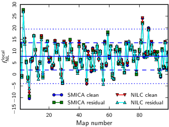
In Sect. 7 we applied our bispectrum estimators to Planck data filtered through four different component separation methods: SMICA, NILC, SEVEM and C-R (for a detailed description of component separation techniques used for Planck see Planck Collaboration XII (2013)). The resulting set of measurements shows very good internal consistency both between different estimators (as expected from our MC validation tests of bispectrum pipelines described in Sect. 6) and between different foreground-cleaned maps. This already makes it clear that foreground residuals in the data are very well under control, and their impact on the final results is only at the level of a small fraction of the measured error bars. In this Section we further investigate this issue, and validate our previous findings on data by running extensive tests in which we compare simulated data sets with and without foreground residuals from two different component separation pipelines, SMICA and NILC. The goal is to provide a MC-based assessment of the expected systematic error from residual foreground contamination.
For each component separation pipeline, we consider two sets of simulations. One set includes realistic Planck noise and beam, is masked and inpainted in the same way as we do for real data, and is processed through SMICA and NILC but it does not contain any foreground component. The other set is obtained by adding to the first one a number of diffuse foreground residuals: thermal and spinning dust components; free-free and synchrotron emission; kinetic and thermal SZ; CO lines and correlated CIB. These residuals have been evaluated by applying the component separation pipelines to accurate synthetic Planck datasets including foreground emission according to the PSM (Delabrouille et al. 2012), and are of course dependent on the cleaning method adopted. The simple procedure of adding foreground residuals to the initially clean simulations is made possible because we consider only linear component separation methods for our analysis. Linearity is in general an important requirement for foreground cleaning algorithms aiming at producing maps suitable for NG analyses. All maps in both samples are lensed using the LensPix algorithm. We analyse both sets using different bispectrum estimators (modal, KSW, binned) for cross-validation purposes.
The presence of residual foreground components in the data can have two main effects on the measured . The first is to introduce a bias in the measurements due to the correlation between the foreground and primordial 3-point function for a given shape. The second is to increase the error bars while leaving the bispectrum estimator asymptotically unbiased. This is a consequence of accidental correlations between primordial CMB anisotropies and foreground emission. Of course these “CMB-CMB-foregrounds” bispectrum terms average to zero but they do not cancel in the bispectrum variance 6-point function. An interesting point to note is that a large foreground three-point function will tend to produce a negative bias in the local bispectrum measurements. That is because foreground emission produces a positive skewness of the CMB temperature distribution (“excess of photons”), and a positive skewness is in turn related to a negative 161616While not rigorous, this argument captures the leading effect since Galactic foregrounds predominantly contaminate large scales. In principle, positively skewed, small scale foreground residuals (), or the negatively skewed SZ effect, can contribute positive bias. Our simulations with foreground residuals demonstrate that these contributions are subdominant. . A large negative is thus a signature of significant foreground contamination in the map. This is indeed what we observe if we consider raw frequency maps with a small Galactic cut, which is why our frequency-by-frequency analysis in Sect. 8.2 was performed using a very large mask. For more details regarding effects of foreground contamination on primordial NG measurements in the context of the WMAP analysis see Yadav & Wandelt 2008 and Senatore et al. 2010.
In our test we built maps contaminated with foreground residuals by simply adding residual components to the clean maps. That means that the difference for the -th realization in the simulated sample exactly quantifies the change in due to foregrounds on that realization. In order to assess the level of residual foreground contamination on primordial and ISW-lensing shapes, first of all we consider the difference between average values and standard deviations of measured from the two map samples for each shape. As shown in Table 21 we find that neither the average nor the standard deviation shows a significant change between the two datasets. That means that foreground residuals are clearly subdominant, as they do not bias the estimator for any shape and they do not increase the variance through spurious correlations with the CMB primordial signal.
We also consider the difference on a map-by-map basis and compute its standard deviation. This is used as an estimate of the expected bias on a single realization due to the presence of residuals. As already expected from the negligible change in the standard deviations of the two samples, the variance of the map-by-map differences is also very small: Table 21 again shows that it is at most about for any given shape, where is the standard deviation for that shape. As an example, in Fig. 23 we show the measured values of for the first 99 maps in both the SMICA and NILC samples, comparing results with and without residuals. It is evident also from this plot that the change in central value due to including residuals is very small. The very good agreement between the two component separation pipelines is also worth notice.
From the study shown here and from the comparison between different component separation methods in Sect. 7, we can thus conclude that the combination of foreground-cleaned maps and sky coverage we adopt in this work provide a very robust choice for studies.
8.5 Impact of HFI time-ordered information processing on NG constraints
Our validation tests are designed to determine whether instrumental or data processing systematics could lead to a spurious detection of primordial NG. Our analysis protocol passes these tests which allows us to rule out this concern with confidence. These validation tests do not exclude the possibility that the extensive processing of HFI time-ordered information (TOI) could somehow remove non-Gaussian signals present on the sky and thus negatively impact Planck’s ability to detect them. If this were true it would weaken the bounds on primordial NG reported here. HFI TOI processing includes glitch fitting, gain drift and correction (ADC non-linearity), 4K cooler line removal, telegraph noise step correction, and TOD filtering to correct for the bolometer time constant (Planck Collaboration VI 2013; Planck Collaboration VII 2013; Planck Collaboration X 2013).
The following facts constitute strong evidence that HFI TOI processing does not remove non-Gaussian signals:
-
1.
Planck’s ISW-lensing bispectrum measurement is consistent with expectations from the LCDM model, and has the right skew- shape. Like NG of local type, this is a squeezed bispectrum template.
-
2.
When frequency maps are combined to maximize the CIB signal, Planck finds a detection of the nearly squeezed CIB-lensing bispectrum, consistent with the CIB 2-point correlations inferred by Planck (Planck Collaboration XXX 2013).
-
3.
Planck detects residual point sources in the SMICA maps at , seen as a bispectrum of equilateral shape at high consistent with the expected skew-spectrum shape (Fig. 2) on the angular scales where residual infrared sources and far infrared background are expected to be the dominant contaminants of the power spectrum according to the foreground residuals in FFP6 simulations of SMICA maps (Fig. E.3 in Planck Collaboration XII 2013).
-
4.
The trispectrum signal imprinted by Planck’s motion with respect to the CMB rest frame is seen at a sensible level and in a plausible direction (Planck Collaboration XXVII 2013).
-
5.
Planck detects the trispectrum signal due to lensing by large scale structure with high significance and in accordance with LCDM predictions based on the Planck parameter likelihood.
-
6.
Fig. 22 shows that we reproduce the WMAP-9 local NG results on those larger angular scales where the WMAP-9 data are cosmic variance limited.
We conclude that all the forms of NG that should have been seen by Planck have been seen, in quantitative agreement with the expected level across the entire range of angular scales probed. While it cannot be excluded with absolute certainty that some unknown aspect of HFI TOI processing could have affected some unknown form of NG, the presence of these non-Gaussian features in the resulting maps (in addition to signals such as the extracted map of y-distortion, and galactic and extragalactic foregrounds), gives us confidence in the force of the bounds on primordial NG described in this paper.
9 Implications for early Universe physics
The NG analyses performed in this paper show that Planck data are consistent with Gaussian primordial fluctuations. The standard models of single-field slow-roll inflation have therefore survived the most stringent tests of Gaussianity performed to date. On the other hand, the NG constraints obtained on different primordial bispectrum shapes (e.g., local, equilateral and orthogonal), after properly accounting for various contaminants, severely limit various classes of mechanisms for the generation of the primordial perturbations proposed as alternatives to the standard models of inflation.
In the following subsections, unless explicitly stated otherwise, we translate limits on NG to limits on parameters of the theories by constructing a posterior assuming the following: the sampling distribution is Gaussian (which is supported by Gaussian simulations); the likelihood is approximated by the sampling distribution but centred on the NG estimate (see Elsner & Wandelt 2009); uniform or Jeffreys’ prior (where stated), over ranges which are physically meaningful, or as otherwise stated. Where two parameters are involved, the posterior is marginalized to give one-dimensional constraints on the parameter of interest.
9.1 General single-field models of inflation
DBI models: The constraints on provide constraints on the sound speed with which the inflaton fluctuations can propagate during inflation. For example, for DBI models of inflation (Silverstein & Tong 2004; Alishahiha et al. 2004), where the inflaton field features a non-standard kinetic term, the predicted value of the nonlinearity parameter is (Silverstein & Tong 2004; Alishahiha et al. 2004; Chen et al. 2007b). Although very similar to the equilateral shape, we have obtained constraints directly on the theoretical (nonseparable) predicted shape (Eq. 2.1)). The constraint at CL (see Eq. (7.3.1)) implies
| (101) |
The DBI class contains two possibilities based on string constructions. In ultraviolet (UV) DBI models, the inflaton field moves under a quadratic potential from the UV side of a warped background to the infrared side. It is known that this case is already at odds with observations, if theoretical internal consistency of the model and constraints on power spectra and primordial NG are taken into account (Baumann & McAllister 2007; Lidsey & Huston 2007; Bean et al. 2007; Peiris et al. 2007). Our results strongly limit the relativistic régime of these models even without applying the theoretical consistency constraints.
It is therefore interesting to look at infrared (IR) DBI models (Chen 2005b, a) where the inflaton field moves from the IR to the UV side, and the inflaton potential is , with a wide range allowed in principle. In previous work (Bean et al. 2008) a 95% CL limit of was obtained using WMAP. In a minimal version of IR DBI, where stringy effects are neglected and the usual field theory computation of the primordial curvature perturbation holds, one finds (Chen 2005c; Chen et al. 2007b) , , where is the number of -folds; further, primordial NG of the equilateral type is generated with an amplitude . For this model, the range is compatible with Planck’s limits on (Planck Collaboration XXII 2013). Marginalizing over , we find
| (102) |
dramatically restricting the allowed parameter space of this model.
Power-law -inflation: These models (Armendariz-Picon et al. 1999; Chen et al. 2007b) predict , where , . Assuming a prior of , our constraint at CL (see Table 9) leads to the limit at 95% CL. On the other hand, Planck’s constraint on yields the limit (Planck Collaboration XXII 2013). These conflicting limits severely constrain this class of models.
Flat Models and higher derivative interactions: Flat NG can characterize inflationary models which arise from independent interaction terms different from the and discussed in Sect. 2 (see also Sect. 9.2). An example is given by models of inflation based on a Galilean symmetry (Creminelli et al. 2011a), where one of the inflaton cubic interaction terms allowed by the Galilean symmetry, , contributes to the flat bispectrum with an amplitude (Creminelli et al. 2011a). Here, is the relevant inflaton scalar degree of freedom, the usual slow-roll parameter and the scale factor and the Hubble parameter during inflation. Our constraint at CL (see Table 11) leads to at CL. These interaction terms are similar to those arising in general inflaton field models that include extrinsic curvature terms, e.g., parameterized in the Effective Field Theory approach as (Bartolo et al. 2010a), which contribute to a flat bispectrum with an amplitude . In this case, we obtain at CL.
9.2 Implications for Effective Field Theory of Inflation
The effective field theory approach to inflation (Weinberg 2008; Cheung et al. 2008) provides a general way to scan the NG parameter space of inflationary perturbations. For example, one can expand the Lagrangian of the dynamically relevant degrees of freedom into the dominant operators satisfying some underlying symmetries. We will focus on general single-field models parametrized by the following operators (up to cubic order)
where is the scalar degree of freedom (). The measurements on and can be used to constrain the magnitude of the inflaton interaction terms and which give respectively and (Senatore et al. 2010, see also Chen et al. 2007b; Chen 2010b). These two operators give rise to shapes that peak in the equilateral configuration that are, nevertheless, slightly different, so that the total NG signal will be a linear combination of the two, possibly leading also to an orthogonal shape. There are two relevant NG parameters, , the sound speed of the the inflaton fluctuations, and which characterizes the amplitude of the other operator . Following Senatore et al. (2010) we will focus on the dimensionless parameter . For example, DBI inflationary models corresponds to , while the non-interacting model (vanishing NG) correspond to and (or ).
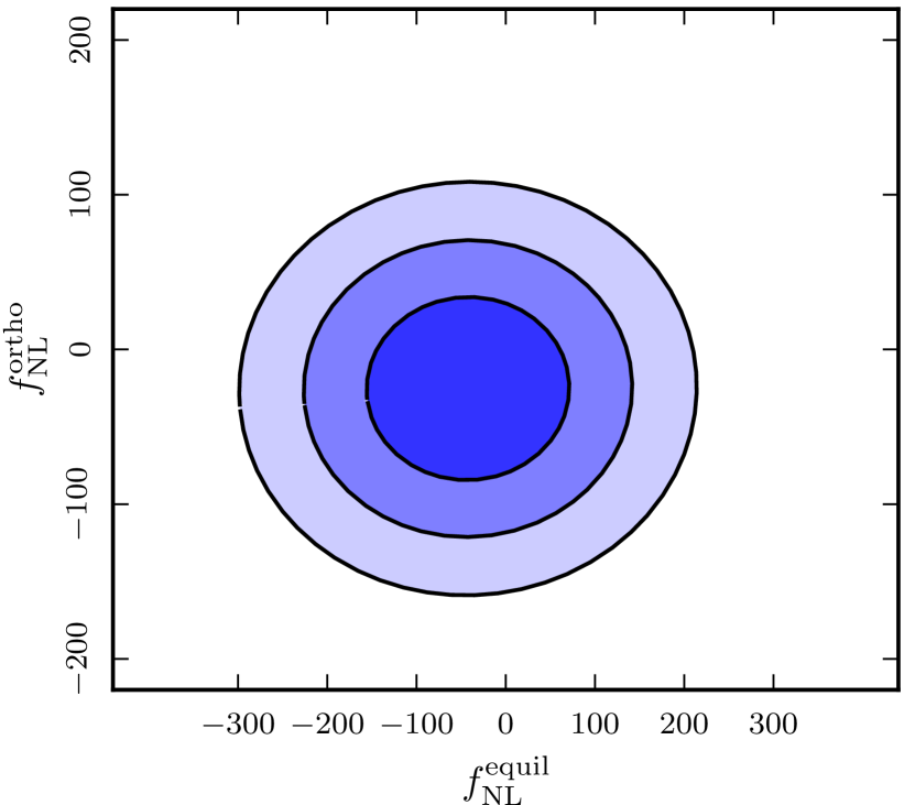
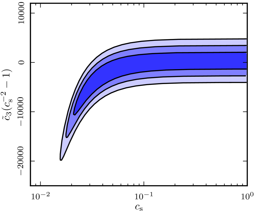
The mean values of the estimators for equilateral and orthogonal NG amplitudes are given in terms of and by
| (104) |
where , and the coefficients are computed from the Fisher correlation matrix between the equilateral and orthogonal template bispectra and the theoretical bispectra arising from the two operators and . Given our constraints on and , and the covariance matrix of the joint estimators, we can define a statistic given by , where the vector is given by . , where ={equilateral, orthogonal}, are the joint estimates of the equilateral and orthogonal measured by Planck and is given by Eq. (9.2). Figure 24 shows the , and confidence regions for and , obtained by requiring , and respectively, as appropriate for a variable with two degrees of freedom. The corresponding confidence regions in the parameter space are shown in Fig. 25. After marginalizing over we find the following conservative bound on the inflaton sound-speed
| (105) |
9.3 Multi-field models
Curvaton models: Planck NG constraints have interesting implications for the simplest adiabatic curvaton models. They predict (Bartolo et al. 2004d, c)
| (106) |
for a quadratic potential of the curvaton field (Lyth & Wands 2002; Lyth et al. 2003; Lyth & Rodriguez 2005; Malik & Lyth 2006; Sasaki et al. 2006), where is the “curvaton decay fraction” evaluated at the epoch of the curvaton decay in the sudden decay approximation. Assuming a prior , given our constraint at 68% CL, we obtain
| (107) |
In Planck Collaboration XXII (2013) a limit on is derived from the constraints on isocurvature perturbations under the assumption that there is some residual isocurvature fluctuations in the curvaton field. For this restricted case, they find ( CL), compatible with the constraint obtained here.
Quasi-single field inflation: It is beyond the scope of this paper to perform a general multi-field analysis employing the local NG constraints. However, we have performed a detailed analysis for the quasi-single field models (see Eq. (12)). Quasi-single field (QSF) inflation models (Chen & Wang 2010b, a; Baumann & Green 2012) are a natural consequence of inflation model-building in string theory and supergravity (see Sect. 2.2). In addition to the inflaton field, these models have extra fields with masses of order the Hubble parameter, which are stabilized by supersymmetry. A distinctive observational signature of these massive fields is a one-parameter family of large NG whose squeezed limits interpolate between the local and the equilateral shape. Therefore, by measuring the precise momentum-dependence of the squeezed configurations in the NG, in principle, we are directly measuring the parameters of the theory naturally determined by the fundamental principle of supersymmetry. These models produce a bispectrum (Eq. (12)) depending on two parameters , , with a shape that interpolates between the local shape, where and the equilateral shape, where .
Results are shown in Fig. 26 (see Sect. 7.3.6 for details of the analyses). The best fit value corresponds to , which would imply, within this scenario, that the extra field different from the inflaton has a mass . However, the figure shows that there is no preferred value for with all values allowed at .
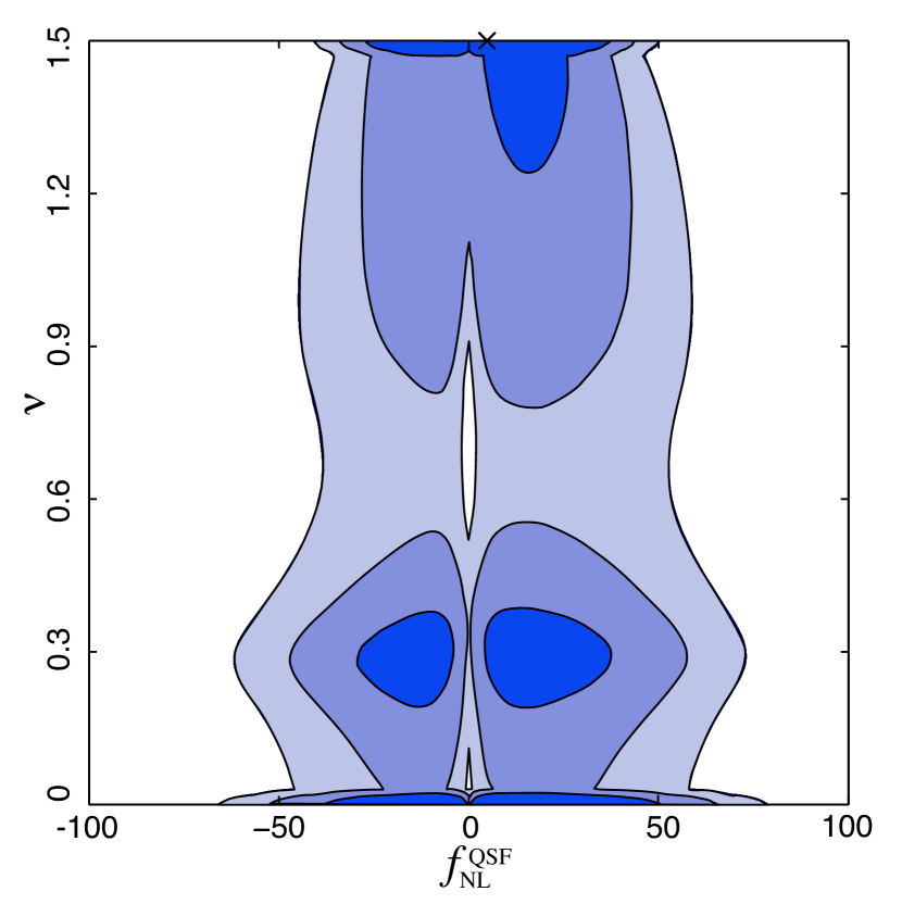
9.4 Non-standard inflation models
Constraints on excited initial states: Results from Sect. 7.3 constrain a variety of models with flattened bispectra, often in combination with a non-trivial squeezed limit. The most notable examples are bispectra produced in excited initial state models (non-Bunch-Davies vacua), which can be generated by strong disturbances away from background slow-roll evolution or additional trans-Planckian physics (Chen et al. 2007b; Holman & Tolley 2008; Meerburg et al. 2009; Agullo & Parker 2011). The constraints we have obtained are summarized in Table 11, and cover four representative cases (see Eq. (14, 15)) in the literature. We find no strong evidence for these flattened bispectra in the Planck data after subtraction of the ISW-lensing signal, with which all these models have some correlation. This is consistent with an earlier constraint on the NBD model from WMAP (Fergusson et al. 2012). However, this investigation is limited by the present resolution of the polynomial modal estimator (), so more strongly flattened models are not excluded by this analysis.
Directional dependence motivated by fields: Directionally-dependent bispectra (Eq. (19)), motivated by inflation with gauge fields, have also been constrained (see Table 11). For example, models with a kinetic term of the vector field(s) , where is the strength of the gauge field, and is a function of the inflaton field which, with an appropriate time dependence (see, e.g., Ratra 1992), can generate vector fields during inflation. For these models the modes in the bispectrum are excited with , where and , respectively (Barnaby et al. 2012a; Bartolo et al. 2013; Shiraishi et al. 2013). Here is the amplitude of a quadrupolar anisotropy in the power spectrum (see, e.g., Ackerman et al. (2007)) and is the number of -folds before the end of inflation when the relevant scales exit the horizon. These modes therefore relate the bispectrum amplitude to the level of statistical anisotropy in the power spectrum. Marginalizing over a prior assuming uniform priors on , our constraints in Table 11 lead to the limits and from the , modes respectively ( CL). Note, however, that in the current analysis only a modest correlation was possible with the shape corresponding to the mode. These results apply to all models where curvature perturbations are sourced by a term (see references in Shiraishi et al. 2013).
Feature models: Non-scale-invariant oscillatory bispectrum shapes can be generated by sharp or periodic features in the inflaton potential, with particular recent interest on axion monodromy models motivated by string theory (see Sect. 2.3). We have undertaken a survey of simple feature models (Eq. (16)) which have a periodicity accessible to the polynomial modal estimator (wavenumbers ), a two-parameter space spanned by and a phase . There are interesting best fit models for the Planck CMB bispectrum around , (that is, with a large- bispectrum periodicity around ), with results shown in Table 12. We note important caveats on the statistics of parameter surveys like this in Sect. 7.3.3; given the large numbers of feature models studied, we have to apply a higher threshold for statistical significance as shown for a survey of 200 Gaussian simulations. This feature survey takes forward earlier results for the WMAP data (Fergusson et al. 2012), with the apparent fit reflecting the signal observed in the Planck CMB reconstruction (see Fig. 7). Most attention on feature models has been motivated by the simplest single-field case for which there are correlated signals predicted in the bispectrum and power spectrum (see e.g., Chen et al. 2007a; Adshead et al. 2012). In this case, regions with small are favoured for producing an observable bispectrum171717Planck Collaboration XVI (2013) confirms an anomaly in the power spectrum at first noted in WMAP, which leads to an improvement in likelihood when fitted with a feature in the inflationary potential (Peiris et al. 2003). Unfortunately, the best-fit parameters in this case do not lead to an observable bispectrum (Adshead et al. 2011)., given existing WMAP power spectrum constraints on these models. Periodicities are anticipated (see Adshead et al. 2012) which are not accessible to the present modal bispectrum estimator analysis, but which are discussed in (Planck Collaboration XXII 2013). Conversely, the Planck feature model survey using the power spectrum (Planck Collaboration XXII 2013) does cover bispectrum scales and parameters investigated in this paper. An analysis of the Bayesian posterior probability (Planck Collaboration XXII 2013) does not appear to provide evidence favoring parameters associated with the current best-fit bispectrum model. More detailed analysis using the specific bispectrum envelope for the single-field feature solution is being undertaken.
Resonance models: We have also investigated resonance models of Eq. (17) such as axion monodromy and enfolded resonance models of Eq. (2.3), in which non-Bunch-Davies vacua are excited by sharp features. This limited analysis focuses on periodicities associated with the best-fit feature model and the results are described in Tables 22 and 23. No significant signal was found in this domain for either of these two models. However, we note that the logarithmic dependence of the bispectrum creates challenges at low , as we must ensure important features do not fall below the modal resolution. This restricts the present survey range, which will be extended in future. Again, we note that most attention on these models has focused on higher -periodicities than those accessible to the present modal estimator (see e.g., Flauger & Pajer 2011; Peiris et al. 2013), for the same reason as the feature models. A resonance model survey using the Planck power spectrum has been undertaken and the results can be found in Planck Collaboration XXII (2013); however, this also currently excludes high frequencies that have received attention in the literature.
Warm inflation: This model, where dissipative effects are important, predicts (Moss & Xiong 2007) where the dissipation parameter must be large for strong dissipation. The limit from WMAP is (Moss & Xiong 2007). Assuming a prior , our constraint at 68% CL (see Sect. 7.3.5) yields a limit on the dissipation parameter of ( CL), improving the previous limit by nearly two orders of magnitude. The strongly-dissipative regime with still remains viable; however, the Planck constraint puts the model in a regime which can lead to an overproduction of gravitinos (see Hall & Peiris (2008) and references within).
9.5 Alternatives to inflation
Perhaps the most striking example is given by the ekpyrotic/cyclic models (for a review, see Lehners 2010) proposed as alternative to inflationary models. Typically they predict a local NG . In particular, the so-called “ekpyrotic conversion” mechanism (in which isocurvature perturbations are converted into curvature perturbations during the ekpyrotic phase) yields , where is a parameter in the potential, requiring for compatibility with power spectrum constraints. This case was discrepant with WMAP data, and with Planck it is decisively ruled out given our bounds at CL (see Table 9) yielding at 95% CL. The predictions for the local bispectrum from other ekpyrotic models (based on the so called “kinetic conversion” taking place after the ekpyrotic phase) yield , where values and are natural (Lehners 2010). Taking , in this case we obtain and at 95% CL, for the plus and minus sign in respectively, significantly restricting the viable parameter space of this model.
9.6 Implications of CMB trispectrum results
The non-detection of local-type by Planck raises the immediate question of whether there might still be a large trispectrum. In this first analysis we have focused on the local shape . Most inflation models predict (Byrnes et al. 2006; Elliston et al. 2012), and hence given our tight limits, would be predicted to be very small. This is easily consistent with our conservative upper limit , and also with the significantly smaller signals found in the modulation dipole and quadrupole. Our upper limit also restricts the freedom of curvaton-like models with quadratic terms that are nearly uncorrelated with the curvature perturbation, which could in principle have but a large trispectrum (Byrnes & Choi 2010).
10 Conclusions
In this paper we have derived constraints on primordial NG, using the CMB maps derived from the Planck nominal mission data. Using three optimal bispectrum estimators – KSW, binned, and modal – we obtained consistent values for the primordial local, equilateral, and orthogonal bispectrum amplitudes, quoting as our final result , , and ( CL statistical). Hence there is no evidence for primordial NG of one of these shapes. We did, however, measure the ISW-lensing bispectrum expected in the scenario, as well as a contribution from diffuse point sources, and these contributions are clearly seen in the form of the associated skew-. Indeed, the detection of ISW-lensing and Poisson point source skew- with the right shapes and at expected levels is good evidence that the data processing is not destroying non-gaussianity in the maps, and gives confidence that the non-detections of primordial non-gaussianity are robust. These results have been confirmed by measurements using the wavelet bispectrum, and Minkowski functional estimators, and demonstrated to be stable for the four different component separation techniques SMICA, NILC, SEVEM, and C-R, showing their robustness against foreground residuals. They have also passed an extensive suite of tests studying the dependence on the maximum multipole number and the mask, consistency checks between frequency channels, and several null tests. In addition, we have summarized in this paper an extensive validation campaign for the three optimal bispectrum estimators on Gaussian and non-Gaussian simulations.
Extending our analysis beyond estimates of individual shape amplitudes, we presented model-independent, three-dimensional reconstructions of the Planck CMB bispectrum using the modal and binned bispectrum estimators. These results were also shown to be fully consistent between the different component separation techniques even for the full bispectrum, and contained no significant NG signals of a type not captured by our standard templates at low multipole values. At high multipoles, some indications of unidentified NG signals were found, as also evidenced by the results from the skew- estimator. Further study will be required to ascertain whether these indications are due to foreground residuals, beams, data processing, or a more interesting signal.
Using the modal decomposition, we have presented constraints on key primordial NG scenarios, including general single-field models with non-separable shapes, excited initial states (non-Bunch-Davies vacua), and directionally-dependent vector models. We have also undertaken an initial survey of scale-dependent feature and resonance models.
Moving beyond three-point correlations, we have obtained limits from the Planck data on the amplitude of the local four-point function. Our trispectrum reconstruction yielded a signal consistent with zero except for an anomalously large octopole. Frequency dependence indicated that this was unlikely to be primordial, but allowing the signal to be primordial we placed an upper limit ( CL).
We have discussed the impact of these results on the inflationary model space, and derived bispectrum constraints on a selection of specific inflationary mechanisms, including both general single-field inflationary models (extensions to the standard single-field slow-roll case) and multi-field models. Our results led to a lower bound on the speed of sound, ( CL), in an effective field theory approach to inflationary models which includes models with non-standard kinetic terms. Strong constraints on other scenarios such as IR DBI, -inflation, inflationary models involving gauge fields, and warm inflation have been obtained. Within the class of multi-field models, our measurements limit the curvaton decay fraction to ( CL). Ekpyrotic/cyclic scenarios were shown to be under pressure from the Planck data: we robustly ruled out the so-called “ekpyrotic conversion” mechanism, and found that the parameter space of the “kinetic conversion” mechanism is significantly limited.
With these results, the paradigm of standard single-field slow-roll inflation has survived its most stringent tests to-date.
Acknowledgements.
The development of Planck has been supported by: ESA; CNES and CNRS/INSU-IN2P3-INP (France); ASI, CNR, and INAF (Italy); NASA and DoE (USA); STFC and UKSA (UK); CSIC, MICINN, JA and RES (Spain); Tekes, AoF and CSC (Finland); DLR and MPG (Germany); CSA (Canada); DTU Space (Denmark); SER/SSO (Switzerland); RCN (Norway); SFI (Ireland); FCT/MCTES (Portugal); and PRACE (EU). A description of the Planck Collaboration and a list of its members, including the technical or scientific activities in which they have been involved, can be found at http://www.sciops.esa.int/index.php?project=planck&page=Planck_Collaboration. The primary platform for analysis with the modal and KSW estimators was the COSMOS supercomputer, part of the DiRAC HPC Facility supported by STFC and the UK Large Facilities Capital Fund. We gratefully acknowledge IN2P3 Computer Center (http://cc.in2p3.fr) for providing a significant amount of the computing resources and services needed for the analysis with the binned bispectrum estimator. This research used resources of the National Energy Research Scientific Computing Center, which is supported by the Office of Science of the U.S. Department of Energy under Contract No. DE-AC02-05CH11231. We acknowledge the use of resources from the Norewegian national super computing facilities NOTUR. We also acknowledge the IAP magique3 computer facilities as well as the curvaton computer at the Department of Physics of the University of Illinois (Urbana, IL). We further acknowledge the computer resources and technical assistance provided by the Spanish Supercomputing Network nodes at Universidad de Cantabria and Universidad Politécnica de Madrid as well as the support provided by the Advanced Computing and e-Science team at IFCA.References
- Achúcarro et al. (2011) Achúcarro, A., Gong, J.-O., Hardeman, S., Palma, G. A., & Patil, S. P. 2011, J. Cosmology Astropart. Phys., 1, 30, 1010.3693
- Ackerman et al. (2007) Ackerman, L., Carroll, S. M., & Wise, M. B. 2007, Phys. Rev. D, 75, 083502, arXiv:astro-ph/0701357
- Acquaviva et al. (2003) Acquaviva, V., Bartolo, N., Matarrese, S., & Riotto, A. 2003, Nuclear Physics B, 667, 119, arXiv:astro-ph/0209156
- Adshead et al. (2012) Adshead, P., Dvorkin, C., Hu, W., & Lim, E. A. 2012, Phys. Rev. D, 85, 023531, 1110.3050
- Adshead et al. (2011) Adshead, P., Hu, W., Dvorkin, C., & Peiris, H. V. 2011, Phys. Rev. D, 84, 043519, 1102.3435
- Agullo & Parker (2011) Agullo, I. & Parker, L. 2011, General Relativity and Gravitation, 43, 2541, 1106.4240
- Alishahiha et al. (2004) Alishahiha, M., Silverstein, E., & Tong, D. 2004, Phys. Rev. D, 70, 123505, arXiv:hep-th/0404084
- Allen et al. (1987) Allen, T. J., Grinstein, B., & Wise, M. B. 1987, Physics Letters B, 197, 66
- Amendola et al. (2011) Amendola, L., Catena, R., Masina, I., et al. 2011, J. Cosmology Astropart. Phys., 7, 27, 1008.1183
- Antoine & Vandergheynst (1998) Antoine, J.-P. & Vandergheynst, P. 1998, Journal of Mathematical Physics, 39, 3987
- Arkani-Hamed et al. (2004) Arkani-Hamed, N., Creminelli, P., Mukohyama, S., & Zaldarriaga, M. 2004, J. Cosmology Astropart. Phys., 4, 1, arXiv:hep-th/0312100
- Armendariz-Picon et al. (1999) Armendariz-Picon, C., Damour, T., & Mukhanov, V. 1999, Physics Letters B, 458, 209, arXiv:hep-th/9904075
- Arroja et al. (2008) Arroja, F., Mizuno, S., & Koyama, K. 2008, J. Cosmology Astropart. Phys., 8, 15, 0806.0619
- Arroja et al. (2009) Arroja, F., Mizuno, S., Koyama, K., & Tanaka, T. 2009, Phys. Rev. D, 80, 043527, 0905.3641
- Ashoorioon & Shiu (2011) Ashoorioon, A. & Shiu, G. 2011, J. Cosmology Astropart. Phys., 3, 25, 1012.3392
- Assassi et al. (2012) Assassi, V., Baumann, D., & Green, D. 2012, J. Cosmology Astropart. Phys., 11, 47, 1204.4207
- Babich (2005) Babich, D. 2005, Phys. Rev. D, 72, 043003, arXiv:astro-ph/0503375
- Babich et al. (2004) Babich, D., Creminelli, P., & Zaldarriaga, M. 2004, J. Cosmology Astropart. Phys., 8, 9, arXiv:astro-ph/0405356
- Bardeen (1980) Bardeen, J. M. 1980, Phys. Rev. D, 22, 1882
- Barnaby & Cline (2006) Barnaby, N. & Cline, J. M. 2006, Phys. Rev. D, 73, 106012, arXiv:astro-ph/0601481
- Barnaby & Cline (2008) Barnaby, N. & Cline, J. M. 2008, J. Cosmology Astropart. Phys., 6, 30, 0802.3218
- Barnaby et al. (2011) Barnaby, N., Namba, R., & Peloso, M. 2011, J. Cosmology Astropart. Phys., 4, 9, 1102.4333
- Barnaby et al. (2012a) Barnaby, N., Namba, R., & Peloso, M. 2012a, Phys. Rev. D, 85, 123523, 1202.1469
- Barnaby et al. (2012b) Barnaby, N., Pajer, E., & Peloso, M. 2012b, Phys. Rev. D, 85, 023525, 1110.3327
- Barnaby & Peloso (2011) Barnaby, N. & Peloso, M. 2011, Physical Review Letters, 106, 181301, 1011.1500
- Bartolo et al. (2010a) Bartolo, N., Fasiello, M., Matarrese, S., & Riotto, A. 2010a, J. Cosmology Astropart. Phys., 8, 8, 1004.0893
- Bartolo et al. (2010b) Bartolo, N., Fasiello, M., Matarrese, S., & Riotto, A. 2010b, J. Cosmology Astropart. Phys., 9, 35, 1006.5411
- Bartolo et al. (2004a) Bartolo, N., Komatsu, E., Matarrese, S., & Riotto, A. 2004a, Phys. Rep, 402, 103, arXiv:astro-ph/0406398
- Bartolo et al. (2013) Bartolo, N., Matarrese, S., Peloso, M., & Ricciardone, A. 2013, Phys. Rev. D, 87, 023504, 1210.3257
- Bartolo et al. (2002) Bartolo, N., Matarrese, S., & Riotto, A. 2002, Phys. Rev. D, 65, 103505, arXiv:hep-ph/0112261
- Bartolo et al. (2004b) Bartolo, N., Matarrese, S., & Riotto, A. 2004b, J. Cosmology Astropart. Phys., 1, 3, arXiv:astro-ph/0309692
- Bartolo et al. (2004c) Bartolo, N., Matarrese, S., & Riotto, A. 2004c, Physical Review Letters, 93, 231301, arXiv:astro-ph/0407505
- Bartolo et al. (2004d) Bartolo, N., Matarrese, S., & Riotto, A. 2004d, Phys. Rev. D, 69, 043503, arXiv:hep-ph/0309033
- Bartolo et al. (2005) Bartolo, N., Matarrese, S., & Riotto, A. 2005, J. Cosmology Astropart. Phys., 8, 10, arXiv:astro-ph/0506410
- Bartolo et al. (2010c) Bartolo, N., Matarrese, S., & Riotto, A. 2010c, Advances in Astronomy, 2010, 1001.3957
- Bartolo et al. (2012) Bartolo, N., Matarrese, S., & Riotto, A. 2012, J. Cosmology Astropart. Phys., 2, 17, 1109.2043
- Bartolo & Riotto (2009) Bartolo, N. & Riotto, A. 2009, J. Cosmology Astropart. Phys., 3, 17, 0811.4584
- Baumann & Green (2012) Baumann, D. & Green, D. 2012, Phys. Rev. D, 85, 103520, 1109.0292
- Baumann & McAllister (2007) Baumann, D. & McAllister, L. 2007, Phys. Rev. D, 75, 123508, arXiv:hep-th/0610285
- Bean et al. (2008) Bean, R., Chen, X., Peiris, H., & Xu, J. 2008, Phys. Rev. D, 77, 023527, 0710.1812
- Bean et al. (2007) Bean, R., Shandera, S. E., Tye, S.-H. H., & Xu, J. 2007, J. Cosmology Astropart. Phys., 5, 4, arXiv:hep-th/0702107
- Bennett et al. (2012) Bennett, C. L., Larson, D., Weiland, J. L., et al. 2012, ArXiv e-prints, 1212.5225
- Berera (1995) Berera, A. 1995, Physical Review Letters, 75, 3218, arXiv:astro-ph/9509049
- Bernardeau et al. (2004) Bernardeau, F., Kofman, L., & Uzan, J.-P. 2004, Phys. Rev. D, 70, 083004, arXiv:astro-ph/0403315
- Bernardeau & Uzan (2002) Bernardeau, F. & Uzan, J.-P. 2002, Phys. Rev. D, 66, 103506, arXiv:hep-ph/0207295
- Bond et al. (2009) Bond, J. R., Frolov, A. V., Huang, Z., & Kofman, L. 2009, Physical Review Letters, 103, 071301, 0903.3407
- Boubekeur et al. (2009) Boubekeur, L., Creminelli, P., D’Amico, G., Noreña, J., & Vernizzi, F. 2009, J. Cosmology Astropart. Phys., 8, 29, 0906.0980
- Bucher et al. (2010) Bucher, M., van Tent, B., & Carvalho, C. S. 2010, MNRAS, 407, 2193, 0911.1642
- Bucher & Zhu (1997) Bucher, M. & Zhu, Y. 1997, Phys. Rev. D, 55, 7415, arXiv:astro-ph/9610223
- Byrnes & Choi (2010) Byrnes, C. T. & Choi, K.-Y. 2010, Advances in Astronomy, 2010, 1002.3110
- Byrnes et al. (2006) Byrnes, C. T., Sasaki, M., & Wands, D. 2006, Phys. Rev. D, 74, 123519, arXiv:astro-ph/0611075
- Cardoso et al. (2008) Cardoso, J., Martin, M., Delabrouille, J., Betoule, M., & Patanchon, G. 2008, IEEE Journal of Selected Topics in Signal Processing, 2, 735, special issue on Signal Processing for Astronomical and Space Research Applications
- Cayon et al. (2003) Cayon, L., Martínez-González, E., Argueso, F., Banday, A. J., & Gorski, K. M. 2003, MNRAS, 339, 1189, arXiv:astro-ph/0211399
- Challinor & van Leeuwen (2002) Challinor, A. & van Leeuwen, F. 2002, Phys. Rev. D, 65, 103001, arXiv:astro-ph/0112457
- Chambers & Rajantie (2008) Chambers, A. & Rajantie, A. 2008, Physical Review Letters, 100, 041302, 0710.4133
- Chen (2005a) Chen, X. 2005a, Journal of High Energy Physics, 8, 45, arXiv:hep-th/0501184
- Chen (2005b) Chen, X. 2005b, Phys. Rev. D, 71, 063506, arXiv:hep-th/0408084
- Chen (2005c) Chen, X. 2005c, Phys. Rev. D, 72, 123518, arXiv:astro-ph/0507053
- Chen (2010a) Chen, X. 2010a, J. Cosmology Astropart. Phys., 12, 3, 1008.2485
- Chen (2010b) Chen, X. 2010b, Advances in Astronomy, 2010, 1002.1416
- Chen (2011) Chen, X. 2011, Physics Letters B, 706, 111, 1106.1635
- Chen et al. (2007a) Chen, X., Easther, R., & Lim, E. A. 2007a, J. Cosmology Astropart. Phys., 6, 23, arXiv:astro-ph/0611645
- Chen et al. (2008) Chen, X., Easther, R., & Lim, E. A. 2008, J. Cosmology Astropart. Phys., 4, 10, 0801.3295
- Chen et al. (2013) Chen, X., Firouzjahi, H., Namjoo, M. H., & Sasaki, M. 2013, ArXiv e-prints, 1301.5699
- Chen et al. (2009) Chen, X., Hu, B., Huang, M.-x., Shiu, G., & Wang, Y. 2009, J. Cosmology Astropart. Phys., 8, 8, 0905.3494
- Chen et al. (2007b) Chen, X., Huang, M.-x., Kachru, S., & Shiu, G. 2007b, J. Cosmology Astropart. Phys., 1, 2, arXiv:hep-th/0605045
- Chen & Wang (2010a) Chen, X. & Wang, Y. 2010a, Phys. Rev. D, 81, 063511, 0909.0496
- Chen & Wang (2010b) Chen, X. & Wang, Y. 2010b, J. Cosmology Astropart. Phys., 4, 27, 0911.3380
- Cheung et al. (2008) Cheung, C., Fitzpatrick, A. L., Kaplan, J., Senatore, L., & Creminelli, P. 2008, Journal of High Energy Physics, 3, 14, 0709.0293
- Cicoli et al. (2012) Cicoli, M., Tasinato, G., Zavala, I., Burgess, C. P., & Quevedo, F. 2012, J. Cosmology Astropart. Phys., 5, 39, 1202.4580
- Cooray & Hu (2000) Cooray, A. & Hu, W. 2000, ApJ, 534, 533, arXiv:astro-ph/9910397
- Creminelli et al. (2011a) Creminelli, P., D’Amico, G., Musso, M., Noreña, J., & Trincherini, E. 2011a, J. Cosmology Astropart. Phys., 2, 6, 1011.3004
- Creminelli et al. (2006) Creminelli, P., Nicolis, A., Senatore, L., Tegmark, M., & Zaldarriaga, M. 2006, J. Cosmology Astropart. Phys., 5, 4, arXiv:astro-ph/0509029
- Creminelli et al. (2011b) Creminelli, P., Pitrou, C., & Vernizzi, F. 2011b, J. Cosmology Astropart. Phys., 11, 25, 1109.1822
- Creminelli & Zaldarriaga (2004a) Creminelli, P. & Zaldarriaga, M. 2004a, J. Cosmology Astropart. Phys., 10, 6, arXiv:astro-ph/0407059
- Creminelli & Zaldarriaga (2004b) Creminelli, P. & Zaldarriaga, M. 2004b, Phys. Rev. D, 70, 083532, arXiv:astro-ph/0405428
- Cruz et al. (2007) Cruz, M., Cayon, L., Martínez-González, E., Vielva, P., & Jin, J. 2007, ApJ, 655, 11, arXiv:astro-ph/0603859
- Curto et al. (2008) Curto, A., Macias-Perez, J. F., Martínez-González, E., et al. 2008, A&A, 486, 383, 0804.0136
- Curto et al. (2009a) Curto, A., Martínez-González, E., & Barreiro, R. B. 2009a, ApJ, 706, 399, 0902.1523
- Curto et al. (2011a) Curto, A., Martínez-González, E., & Barreiro, R. B. 2011a, MNRAS, 412, 1038, 1007.2181
- Curto et al. (2012) Curto, A., Martínez-González, E., & Barreiro, R. B. 2012, MNRAS, 426, 1361, 1111.3390
- Curto et al. (2011b) Curto, A., Martínez-González, E., Barreiro, R. B., & Hobson, M. P. 2011b, MNRAS, 417, 488, 1105.6106
- Curto et al. (2009b) Curto, A., Martínez-González, E., Mukherjee, P., et al. 2009b, MNRAS, 393, 615, 0807.0231
- Curto et al. (2013) Curto, A., Tucci, M., González-Nuevo, J., et al. 2013, ArXiv e-prints, 1301.1544
- De Troia et al. (2007) De Troia, G., Ade, P. A. R., Bock, J. J., et al. 2007, ApJ, 670, L73
- Delabrouille et al. (2012) Delabrouille, J., Betoule, M., Melin, J.-B., et al. 2012, ArXiv e-prints, 1207.3675
- Delabrouille et al. (2009) Delabrouille, J., Cardoso, J., Le Jeune, M., et al. 2009, A&A, 493, 835, 0807.0773
- Delabrouille et al. (2003) Delabrouille, J., Cardoso, J.-F., & Patanchon, G. 2003, MNRAS, 346, 1089, arXiv:astro-ph/0211504
- Donzelli et al. (2009) Donzelli, S., Hansen, F. K., Liguori, M., & Maino, D. 2009, ApJ, 706, 1226, 0907.4650
- Donzelli et al. (2012) Donzelli, S., Hansen, F. K., Liguori, M., Marinucci, D., & Matarrese, S. 2012, ApJ, 755, 19, 1202.1478
- Ducout et al. (2013) Ducout, A., Bouchet, F. R., Colombi, S., Pogosyan, D., & Prunet, S. 2013, MNRAS, 429, 2104, 1209.1223
- Dvali et al. (2004a) Dvali, G., Gruzinov, A., & Zaldarriaga, M. 2004a, Phys. Rev. D, 69, 083505, arXiv:astro-ph/0305548
- Dvali et al. (2004b) Dvali, G., Gruzinov, A., & Zaldarriaga, M. 2004b, Phys. Rev. D, 69, 023505, arXiv:astro-ph/0303591
- Elliston et al. (2012) Elliston, J., Alabidi, L., Huston, I., Mulryne, D., & Tavakol, R. 2012, J. Cosmology Astropart. Phys., 9, 1, 1203.6844
- Elsner & Wandelt (2009) Elsner, F. & Wandelt, B. D. 2009, ApJS, 184, 264, 0909.0009
- Elsner & Wandelt (2013) Elsner, F. & Wandelt, B. D. 2013, A&A, 549, A111, 1210.4931
- Endlich et al. (2012) Endlich, S., Nicolis, A., & Wang, J. 2012, ArXiv e-prints, 1210.0569
- Enqvist et al. (2005) Enqvist, K., Jokinen, A., Mazumdar, A., Multamäki, T., & Väihkönen, A. 2005, Physical Review Letters, 94, 161301, arXiv:astro-ph/0411394
- Enqvist & Sloth (2002) Enqvist, K. & Sloth, M. S. 2002, Nuclear Physics B, 626, 395, arXiv:hep-ph/0109214
- Eriksen et al. (2006) Eriksen, H. K., Dickinson, C., Lawrence, C. R., et al. 2006, ApJ, 641, 665, arXiv:astro-ph/0508268
- Eriksen et al. (2008) Eriksen, H. K., Jewell, J. B., Dickinson, C., et al. 2008, ApJ, 676, 10, 0709.1058
- Eriksen et al. (2004) Eriksen, H. K., Novikov, D. I., Lilje, P. B., Banday, A. J., & Górski, K. M. 2004, ApJ, 612, 64, arXiv:astro-ph/0401276
- Falk et al. (1993) Falk, T., Rangarajan, R., & Srednicki, M. 1993, ApJ, 403, L1, arXiv:astro-ph/9208001
- Faÿ et al. (2008) Faÿ, G., Guilloux, F., Betoule, M., et al. 2008, Phys. Rev. D, 78, 083013, 0807.1113
- Feeney et al. (2011) Feeney, S. M., Johnson, M. C., Mortlock, D. J., & Peiris, H. V. 2011, Phys. Rev. D, 84, 043507, 1012.3667
- Fergusson et al. (2010a) Fergusson, J. R., Liguori, M., & Shellard, E. P. S. 2010a, Phys. Rev. D, 82, 023502, 0912.5516
- Fergusson et al. (2012) Fergusson, J. R., Liguori, M., & Shellard, E. P. S. 2012, J. Cosmology Astropart. Phys., 12, 32, 1006.1642
- Fergusson et al. (2010b) Fergusson, J. R., Regan, D. M., & Shellard, E. P. S. 2010b, ArXiv e-prints, 1012.6039
- Fergusson & Shellard (2007) Fergusson, J. R. & Shellard, E. P. S. 2007, Phys. Rev. D, 76, 083523, arXiv:astro-ph/0612713
- Fernández-Cobos et al. (2012) Fernández-Cobos, R., Vielva, P., Barreiro, R. B., & Martínez-González, E. 2012, MNRAS, 420, 2162, 1106.2016
- Ferreira & Magueijo (1997) Ferreira, P. G. & Magueijo, J. 1997, Phys. Rev. D, 56, 4578, arXiv:astro-ph/9704052
- Flauger et al. (2010) Flauger, R., McAllister, L., Pajer, E., Westphal, A., & Xu, G. 2010, J. Cosmology Astropart. Phys., 6, 9, 0907.2916
- Flauger & Pajer (2011) Flauger, R. & Pajer, E. 2011, J. Cosmology Astropart. Phys., 1, 17, 1002.0833
- Gangui et al. (1994) Gangui, A., Lucchin, F., Matarrese, S., & Mollerach, S. 1994, ApJ, 430, 447, arXiv:astro-ph/9312033
- Gangui & Martin (2000a) Gangui, A. & Martin, J. 2000a, Phys. Rev. D, 62, 103004, arXiv:astro-ph/0001361
- Gangui & Martin (2000b) Gangui, A. & Martin, J. 2000b, MNRAS, 313, 323, arXiv:astro-ph/9908009
- Geller & Mayeli (2009a) Geller, D. & Mayeli, A. 2009a, Math. Z., 262, 895
- Geller & Mayeli (2009b) Geller, D. & Mayeli, A. 2009b, Math. Z., 263, 235
- Giovi et al. (2005) Giovi, F., Baccigalupi, C., & Perrotta, F. 2005, Phys. Rev. D, 71, 103009, arXiv:astro-ph/0411702
- Goldberg & Spergel (1999) Goldberg, D. M. & Spergel, D. N. 1999, Phys. Rev. D, 59, 103002, arXiv:astro-ph/9811251
- González-Nuevo et al. (2005) González-Nuevo, J., Toffolatti, L., & Argüeso, F. 2005, ApJ, 621, 1, arXiv:astro-ph/0405553
- Górski et al. (2005) Górski, K. M., Hivon, E., Banday, A. J., et al. 2005, ApJ, 622, 759, arXiv:astro-ph/0409513
- Green et al. (2009) Green, D., Horn, B., Senatore, L., & Silverstein, E. 2009, Phys. Rev. D, 80, 063533, 0902.1006
- Hall & Peiris (2008) Hall, L. M. H. & Peiris, H. V. 2008, J. Cosmology Astropart. Phys., 1, 27, 0709.2912
- Hamimeche & Lewis (2008) Hamimeche, S. & Lewis, A. 2008, Phys. Rev. D, 77, 103013, 0801.0554
- Hanson & Lewis (2009) Hanson, D. & Lewis, A. 2009, Phys. Rev. D, 80, 063004, 0908.0963
- Hanson et al. (2009a) Hanson, D., Rocha, G., & Górski, K. 2009a, MNRAS, 400, 2169, 0907.1927
- Hanson et al. (2009b) Hanson, D., Smith, K. M., Challinor, A., & Liguori, M. 2009b, Phys. Rev. D, 80, 083004, 0905.4732
- Heavens (1998) Heavens, A. F. 1998, MNRAS, 299, 805, arXiv:astro-ph/9804222
- Hikage et al. (2006) Hikage, C., Komatsu, E., & Matsubara, T. 2006, ApJ, 653, 11, arXiv:astro-ph/0607284
- Hikage & Matsubara (2012) Hikage, C. & Matsubara, T. 2012, MNRAS, 425, 2187, 1207.1183
- Hikage et al. (2008) Hikage, C., Matsubara, T., Coles, P., et al. 2008, MNRAS, 389, 1439, 0802.3677
- Hodges et al. (1990) Hodges, H. M., Blumenthal, G. R., Kofman, L. A., & Primack, J. R. 1990, Nuclear Physics B, 335, 197
- Holman & Tolley (2008) Holman, R. & Tolley, A. J. 2008, J. Cosmology Astropart. Phys., 5, 1, 0710.1302
- Huang & Shiu (2006) Huang, M. X. & Shiu, G. 2006, Phys. Rev. D, 74, 121301, arXiv:hep-th/0610235
- Huang & Vernizzi (2013) Huang, Z. & Vernizzi, F. 2013, Physical Review Letters, 110, 101303, 1212.3573
- Izumi et al. (2012) Izumi, K., Mizuno, S., & Koyama, K. 2012, Phys. Rev. D, 85, 023521, 1109.3746
- Junk & Komatsu (2012) Junk, V. & Komatsu, E. 2012, Phys. Rev. D, 85, 123524, 1204.3789
- Kehagias & Riotto (2012) Kehagias, A. & Riotto, A. 2012, ArXiv e-prints, 1205.1523
- Keihänen et al. (2010) Keihänen, E., Keskitalo, R., Kurki-Suonio, H., Poutanen, T., & Sirviö, A. 2010, A&A, 510, A57+, 0907.0367
- Khatri & Wandelt (2009) Khatri, R. & Wandelt, B. D. 2009, Phys. Rev. D, 79, 023501, 0810.4370
- Khatri & Wandelt (2010) Khatri, R. & Wandelt, B. D. 2010, Phys. Rev. D, 81, 103518, 0903.0871
- Kim et al. (2013) Kim, J., Rotti, A., & Komatsu, E. 2013, ArXiv e-prints, 1302.5799
- Kofman (2003) Kofman, L. 2003, ArXiv Astrophysics e-prints, arXiv:astro-ph/0303614
- Kofman et al. (1991) Kofman, L., Blumenthal, G. R., Hodges, H., & Primack, J. R. 1991, in Astronomical Society of the Pacific Conference Series, Vol. 15, Large-scale Structures and Peculiar Motions in the Universe, ed. D. W. Latham & L. A. N. da Costa, 339
- Kogo & Komatsu (2006) Kogo, N. & Komatsu, E. 2006, Phys. Rev. D, 73, 083007, arXiv:astro-ph/0602099
- Kolb et al. (2006) Kolb, E. W., Riotto, A., & Vallinotto, A. 2006, Phys. Rev. D, 73, 023522, arXiv:astro-ph/0511198
- Komatsu (2010) Komatsu, E. 2010, Classical and Quantum Gravity, 27, 124010, 1003.6097
- Komatsu et al. (2009) Komatsu, E., Dunkley, J., Nolta, M. R., et al. 2009, ApJS, 180, 330, 0803.0547
- Komatsu et al. (2003) Komatsu, E., Kogut, A., Nolta, M. R., et al. 2003, ApJS, 148, 119, arXiv:astro-ph/0302223
- Komatsu et al. (2011) Komatsu, E., Smith, K. M., Dunkley, J., et al. 2011, ApJS, 192, 18, 1001.4538
- Komatsu & Spergel (2001) Komatsu, E. & Spergel, D. N. 2001, Phys. Rev. D, 63, 063002, arXiv:astro-ph/0005036
- Komatsu et al. (2005) Komatsu, E., Spergel, D. N., & Wandelt, B. D. 2005, ApJ, 634, 14, arXiv:astro-ph/0305189
- Kosowsky & Kahniashvili (2011) Kosowsky, A. & Kahniashvili, T. 2011, Physical Review Letters, 106, 191301, 1007.4539
- Lacasa & Aghanim (2012) Lacasa, F. & Aghanim, N. 2012, ArXiv e-prints, 1211.3902
- Lacasa et al. (2012) Lacasa, F., Aghanim, N., Kunz, M., & Frommert, M. 2012, MNRAS, 421, 1982, 1107.2251
- Lan & Marinucci (2008) Lan, X. & Marinucci, D. 2008, Electronic Journal of Statistics, 2, 332, 0802.4020
- Langlois et al. (2008a) Langlois, D., Renaux-Petel, S., Steer, D. A., & Tanaka, T. 2008a, Physical Review Letters, 101, 061301, 0804.3139
- Langlois et al. (2008b) Langlois, D., Renaux-Petel, S., Steer, D. A., & Tanaka, T. 2008b, Phys. Rev. D, 78, 063523, 0806.0336
- Leach et al. (2008) Leach, S. M., Cardoso, J., Baccigalupi, C., et al. 2008, A&A, 491, 597, 0805.0269
- Lehners (2010) Lehners, J.-L. 2010, Advances in Astronomy, 2010, 1001.3125
- Lewis (2011) Lewis, A. 2011, J. Cosmology Astropart. Phys., 10, 26, 1107.5431
- Lewis (2012) Lewis, A. 2012, J. Cosmology Astropart. Phys., 6, 23, 1204.5018
- Lewis & Challinor (2006) Lewis, A. & Challinor, A. 2006, Phys. Rep, 429, 1, arXiv:astro-ph/0601594
- Lewis et al. (2011) Lewis, A., Challinor, A., & Hanson, D. 2011, J. Cosmology Astropart. Phys., 3, 18, 1101.2234
- Lidsey & Huston (2007) Lidsey, J. E. & Huston, I. 2007, J. Cosmology Astropart. Phys., 7, 2, 0705.0240
- Lidsey et al. (1997) Lidsey, J. E., Liddle, A. R., Kolb, E. W., et al. 1997, Reviews of Modern Physics, 69, 373, arXiv:astro-ph/9508078
- Liguori et al. (2010) Liguori, M., Sefusatti, E., Fergusson, J. R., & Shellard, E. P. S. 2010, Advances in Astronomy, 2010, 1001.4707
- Linde & Mukhanov (1997) Linde, A. & Mukhanov, V. 1997, Phys. Rev. D, 56, 535, arXiv:astro-ph/9610219
- Lyth (2005) Lyth, D. H. 2005, J. Cosmology Astropart. Phys., 11, 6, arXiv:astro-ph/0510443
- Lyth & Riotto (2006) Lyth, D. H. & Riotto, A. 2006, Physical Review Letters, 97, 121301, arXiv:astro-ph/0607326
- Lyth & Rodriguez (2005) Lyth, D. H. & Rodriguez, Y. 2005, Physical Review Letters, 95, 121302, arXiv:astro-ph/0504045
- Lyth et al. (2003) Lyth, D. H., Ungarelli, C., & Wands, D. 2003, Phys. Rev. D, 67, 023503, arXiv:astro-ph/0208055
- Lyth & Wands (2002) Lyth, D. H. & Wands, D. 2002, Physics Letters B, 524, 5, arXiv:hep-ph/0110002
- Lyth & Riotto (1999) Lyth, D. H. D. H. & Riotto, A. A. 1999, Phys. Rep, 314, 1, arXiv:hep-ph/9807278
- Maldacena (2003) Maldacena, J. 2003, Journal of High Energy Physics, 5, 13, arXiv:astro-ph/0210603
- Malik & Lyth (2006) Malik, K. A. & Lyth, D. H. 2006, J. Cosmology Astropart. Phys., 9, 8, arXiv:astro-ph/0604387
- Malik & Wands (2009) Malik, K. A. & Wands, D. 2009, Phys. Rep, 475, 1, 0809.4944
- Mangilli & Verde (2009) Mangilli, A. & Verde, L. 2009, Phys. Rev. D, 80, 123007, 0906.2317
- Mangilli et al. (2013) Mangilli, A., Wandelt, B., Elsner, F., & Liguori, M. 2013, ArXiv e-prints, 1303.1722
- Martínez-González et al. (2002) Martínez-González, E., Gallegos, J. E., Argüeso, F., Cayon, L., & Sanz, J. L. 2002, MNRAS, 336, 22, arXiv:astro-ph/0111284
- Matsubara (2010) Matsubara, T. 2010, Phys. Rev. D, 81, 083505, 1001.2321
- McEwen et al. (2007a) McEwen, J. D., Vielva, P., Hobson, M. P., Martínez-González, E., & Lasenby, A. N. 2007a, MNRAS, 376, 1211, arXiv:astro-ph/0605122
- McEwen et al. (2007b) McEwen, J. D., Vielva, P., Wiaux, Y., et al. 2007b, Journal of Fourier Analysis and Applications, 13, 495, 0704.3158
- Meerburg et al. (2009) Meerburg, P. D., van der Schaar, J. P., & Stefano Corasaniti, P. 2009, J. Cosmology Astropart. Phys., 5, 18, 0901.4044
- Mitra et al. (2011) Mitra, S., Rocha, G., Górski, K. M., et al. 2011, ApJS, 193, 5, 1005.1929
- Modest et al. (2013) Modest, H. I., Räth, C., Banday, A. J., et al. 2013, MNRAS, 428, 551, 1209.5106
- Mollerach (1990) Mollerach, S. 1990, Phys. Rev. D, 42, 313
- Moroi & Takahashi (2001) Moroi, T. & Takahashi, T. 2001, Physics Letters B, 522, 215, arXiv:hep-ph/0110096
- Moss & Xiong (2007) Moss, I. G. & Xiong, C. 2007, J. Cosmology Astropart. Phys., 4, 7, arXiv:astro-ph/0701302
- Munshi & Heavens (2010) Munshi, D. & Heavens, A. 2010, MNRAS, 401, 2406, 0904.4478
- Munshi et al. (2011) Munshi, D., Heavens, A., Cooray, A., et al. 2011, MNRAS, 412, 1993, 0910.3693
- Natoli et al. (2010) Natoli, P., de Troia, G., Hikage, C., et al. 2010, MNRAS, 408, 1658, 0905.4301
- Nitta et al. (2009) Nitta, D., Komatsu, E., Bartolo, N., Matarrese, S., & Riotto, A. 2009, J. Cosmology Astropart. Phys., 5, 14, 0903.0894
- Okamoto & Hu (2002) Okamoto, T. & Hu, W. 2002, Phys. Rev. D, 66, 063008, arXiv:astro-ph/0206155
- Pearson et al. (2012) Pearson, R., Lewis, A., & Regan, D. 2012, J. Cosmology Astropart. Phys., 3, 11, 1201.1010
- Peebles (1997) Peebles, P. J. E. 1997, ApJ, 483, L1
- Peiris et al. (2007) Peiris, H., Baumann, D., Friedman, B., & Cooray, A. 2007, Phys. Rev. D, 76, 103517, 0706.1240
- Peiris et al. (2013) Peiris, H., Easther, R., & Flauger, R. 2013, ArXiv e-prints, 1303.2616
- Peiris et al. (2003) Peiris, H. V., Komatsu, E., Verde, L., et al. 2003, ApJS, 148, 213
- Pettinari et al. (2013) Pettinari, G. W., Fidler, C., Crittenden, R., Koyama, K., & Wands, D. 2013, ArXiv e-prints, 1302.0832
- Pietrobon et al. (2006) Pietrobon, D., Balbi, A., & Marinucci, D. 2006, Phys. Rev. D, 74, 043524, arXiv:astro-ph/0606475
- Pietrobon et al. (2010) Pietrobon, D., Cabella, P., Balbi, A., et al. 2010, MNRAS, 402, L34, 0905.3702
- Pietrobon et al. (2009) Pietrobon, D., Cabella, P., Balbi, A., de Gasperis, G., & Vittorio, N. 2009, MNRAS, 396, 1682, 0812.2478
- Planck Collaboration ES (2013) Planck Collaboration ES. 2013, The Explanatory Supplement to the Planck 2013 results (ESA)
- Planck Collaboration I (2013) Planck Collaboration I. 2013, Submitted to A&A, [arXiv:astro-ph/1303.5062]
- Planck Collaboration II (2013) Planck Collaboration II. 2013, Submitted to A&A, [arXiv:astro-ph/1303.5063]
- Planck Collaboration IV (2013) Planck Collaboration IV. 2013, Submitted to A&A, [arXiv:astro-ph/1303.5065]
- Planck Collaboration VI (2013) Planck Collaboration VI. 2013, Submitted to A&A, [arXiv:astro-ph/1303.5067]
- Planck Collaboration VII (2013) Planck Collaboration VII. 2013, Submitted to A&A, [arXiv:astro-ph/1303.5068]
- Planck Collaboration VIII (2013) Planck Collaboration VIII. 2013, Submitted to A&A, [arXiv:astro-ph/1303.5069]
- Planck Collaboration X (2013) Planck Collaboration X. 2013, Submitted to A&A, [arXiv:astro-ph/1303.5071]
- Planck Collaboration XII (2013) Planck Collaboration XII. 2013, Submitted to A&A, [arXiv:astro-ph/1303.5072]
- Planck Collaboration XIV (2013) Planck Collaboration XIV. 2013, Submitted to A&A, [arXiv:astro-ph/1303.5074]
- Planck Collaboration XIX (2013) Planck Collaboration XIX. 2013, Submitted to A&A, [arXiv:astro-ph/1303.5079]
- Planck Collaboration XV (2013) Planck Collaboration XV. 2013, Submitted to A&A, [arXiv:astro-ph/1303.5075]
- Planck Collaboration XVI (2013) Planck Collaboration XVI. 2013, Submitted to A&A, [arXiv:astro-ph/1303.5076]
- Planck Collaboration XVII (2013) Planck Collaboration XVII. 2013, Submitted to A&A, [arXiv:astro-ph/1303.5077]
- Planck Collaboration XXII (2013) Planck Collaboration XXII. 2013, Submitted to A&A, [arXiv:astro-ph/1303.5082]
- Planck Collaboration XXIII (2013) Planck Collaboration XXIII. 2013, Submitted to A&A, [arXiv:astro-ph/1303.5083]
- Planck Collaboration XXV (2013) Planck Collaboration XXV. 2013, Submitted to A&A, [arXiv:astro-ph/1303.5085]
- Planck Collaboration XXVII (2013) Planck Collaboration XXVII. 2013, Submitted to A&A, [arXiv:astro-ph/1303.5087]
- Planck Collaboration XXX (2013) Planck Collaboration XXX. 2013, Submitted to A&A, [arXiv:astro-ph/1309.0382]
- Ratra (1992) Ratra, B. 1992, ApJ, 391, L1
- Rees & Sciama (1968) Rees, M. J. & Sciama, D. W. 1968, Nature, 217, 511
- Regan et al. (2013) Regan, D., Mukherjee, P., & Seery, D. 2013, ArXiv e-prints, 1302.5631
- Reinecke et al. (2006) Reinecke, M., Dolag, K., Hell, R., Bartelmann, M., & Enßlin, T. A. 2006, A&A, 445, 373, arXiv:astro-ph/0508522
- Renaux-Petel (2009) Renaux-Petel, S. 2009, J. Cosmology Astropart. Phys., 10, 12, 0907.2476
- Renaux-Petel et al. (2011) Renaux-Petel, S., Mizuno, S., & Koyama, K. 2011, J. Cosmology Astropart. Phys., 11, 42, 1108.0305
- Rigopoulos et al. (2006) Rigopoulos, G. I., Shellard, E. P. S., & van Tent, B. J. W. 2006, Phys. Rev. D, 73, 083522, arXiv:astro-ph/0506704
- Rigopoulos et al. (2007) Rigopoulos, G. I., Shellard, E. P. S., & van Tent, B. J. W. 2007, Phys. Rev. D, 76, 083512, arXiv:astro-ph/0511041
- Rudjord et al. (2009) Rudjord, O., Hansen, F. K., Lan, X., et al. 2009, ApJ, 701, 369, 0901.3154
- Sachs & Wolfe (1967) Sachs, R. K. & Wolfe, A. M. 1967, ApJ, 147, 73
- Salem (2005) Salem, M. P. 2005, Phys. Rev. D, 72, 123516, arXiv:astro-ph/0511146
- Salopek & Bond (1990) Salopek, D. S. & Bond, J. R. 1990, Phys. Rev. D, 42, 3936
- Sasaki et al. (2006) Sasaki, M., Väliviita, J., & Wands, D. 2006, Phys. Rev. D, 74, 103003, arXiv:astro-ph/0607627
- Scodeller et al. (2011) Scodeller, S., Rudjord, O., Hansen, F. K., et al. 2011, ApJ, 733, 121, 1004.5576
- Sefusatti et al. (2012) Sefusatti, E., Fergusson, J. R., Chen, X., & Shellard, E. P. S. 2012, J. Cosmology Astropart. Phys., 8, 33, 1204.6318
- Senatore et al. (2010) Senatore, L., Smith, K. M., & Zaldarriaga, M. 2010, J. Cosmology Astropart. Phys., 1, 28, 0905.3746
- Senatore et al. (2009) Senatore, L., Tassev, S., & Zaldarriaga, M. 2009, J. Cosmology Astropart. Phys., 9, 38, 0812.3658
- Senatore & Zaldarriaga (2011) Senatore, L. & Zaldarriaga, M. 2011, J. Cosmology Astropart. Phys., 1, 3, 1004.1201
- Serra & Cooray (2008) Serra, P. & Cooray, A. 2008, Phys. Rev. D, 77, 107305, 0801.3276
- Shiraishi et al. (2013) Shiraishi, M., Komatsu, E., Peloso, M., & Barnaby, N. 2013, ArXiv e-prints, 1302.3056
- Shiraishi et al. (2012) Shiraishi, M., Nitta, D., Yokoyama, S., & Ichiki, K. 2012, J. Cosmology Astropart. Phys., 3, 41, 1201.0376
- Shiu & Xu (2011) Shiu, G. & Xu, J. 2011, Phys. Rev. D, 84, 103509, 1108.0981
- Silverstein & Tong (2004) Silverstein, E. & Tong, D. 2004, Phys. Rev. D, 70, 103505, arXiv:hep-th/0310221
- Smidt et al. (2010) Smidt, J., Amblard, A., Byrnes, C. T., et al. 2010, Phys. Rev. D, 81, 123007, 1004.1409
- Smith et al. (2011) Smith, K. M., Loverde, M., & Zaldarriaga, M. 2011, Physical Review Letters, 107, 191301, 1108.1805
- Smith et al. (2009) Smith, K. M., Senatore, L., & Zaldarriaga, M. 2009, J. Cosmology Astropart. Phys., 9, 6, 0901.2572
- Smith & Zaldarriaga (2011) Smith, K. M. & Zaldarriaga, M. 2011, MNRAS, 417, 2, arXiv:astro-ph/0612571
- Smith & Kamionkowski (2012) Smith, T. L. & Kamionkowski, M. 2012, Phys. Rev. D, 86, 063009, 1203.6654
- Starck et al. (2006) Starck, J.-L., Moudden, Y., Abrial, P., & Nguyen, M. 2006, A&A, 446, 1191, arXiv:astro-ph/0509883
- Starck et al. (2010) Starck, J.-L., Murtagh, F., & Fadili, J. M. 2010, Sparse image and signal processing (Cambridge: Cambridge University Press), xviii+316, wavelets, curvelets, morphological diversity
- Su et al. (2012) Su, S.-C., Lim, E. A., & Shellard, E. P. S. 2012, ArXiv e-prints, 1212.6968
- Sugiyama (2012) Sugiyama, N. S. 2012, J. Cosmology Astropart. Phys., 5, 32, 1201.4048
- Sugiyama et al. (2011) Sugiyama, N. S., Komatsu, E., & Futamase, T. 2011, Physical Review Letters, 106, 251301, 1101.3636
- Suyama et al. (2010) Suyama, T., Takahashi, T., Yamaguchi, M., & Yokoyama, S. 2010, J. Cosmology Astropart. Phys., 12, 30, 1009.1979
- Suyama & Yamaguchi (2008) Suyama, T. & Yamaguchi, M. 2008, Phys. Rev. D, 77, 023505, 0709.2545
- Toffolatti et al. (1998) Toffolatti, L., Argueso Gomez, F., de Zotti, G., et al. 1998, MNRAS, 297, 117, arXiv:astro-ph/9711085
- Tolley & Wyman (2010) Tolley, A. J. & Wyman, M. 2010, Phys. Rev. D, 81, 043502, 0910.1853
- Tzavara & van Tent (2011) Tzavara, E. & van Tent, B. 2011, J. Cosmology Astropart. Phys., 6, 26, 1012.6027
- Verde et al. (2013) Verde, L., Jimenez, R., Alvarez-Gaume, L., Heavens, A. F., & Matarrese, S. 2013, ArXiv e-prints, 1301.6017
- Verde & Spergel (2002) Verde, L. & Spergel, D. N. 2002, Phys. Rev. D, 65, 043007, arXiv:astro-ph/0108179
- Verde et al. (2000) Verde, L., Wang, L., Heavens, A. F., & Kamionkowski, M. 2000, MNRAS, 313, 141, arXiv:astro-ph/9906301
- Vernizzi & Wands (2006) Vernizzi, F. & Wands, D. 2006, J. Cosmology Astropart. Phys., 5, 19, arXiv:astro-ph/0603799
- Wang & Kamionkowski (2000) Wang, L. & Kamionkowski, M. 2000, Phys. Rev. D, 61, 063504, arXiv:astro-ph/9907431
- Weinberg (2008) Weinberg, S. 2008, Phys. Rev. D, 77, 123541, 0804.4291
- Yadav et al. (2007) Yadav, A. P. S., Komatsu, E., & Wandelt, B. D. 2007, ApJ, 664, 680, arXiv:astro-ph/0701921
- Yadav et al. (2008) Yadav, A. P. S., Komatsu, E., Wandelt, B. D., et al. 2008, ApJ, 678, 578, 0711.4933
- Yadav & Wandelt (2008) Yadav, A. P. S. & Wandelt, B. D. 2008, Physical Review Letters, 100, 181301, 0712.1148
- Yadav & Wandelt (2010) Yadav, A. P. S. & Wandelt, B. D. 2010, Advances in Astronomy, 2010, 1006.0275
- Zaldarriaga (2004) Zaldarriaga, M. 2004, Phys. Rev. D, 69, 043508, arXiv:astro-ph/0306006
- Zeldovich & Sunyaev (1969) Zeldovich, Y. B. & Sunyaev, R. A. 1969, Ap&SS, 4, 301
Appendix A Full Focal Plane Simulations
The purpose of the Full Focal Plane (FFP) simulations is to provide a complete, coherent realization of the full Planck mission (both HFI and LFI) using the best available estimates of its characteristics, including the satellite pointing, the individual detector beams, band passes and noise properties, and the various data flags. Each FFP data set consists of three parts: a fiducial observation of an input sky (including our best estimates of all of the foreground components and a realization of the CMB sky corresponding to a chosen cosmology), together with separate MC realization sets of the CMB and noise. The maps made from these simulated data are used both to validate and verify the analysis algorithms and their implementations and to quantify uncertainties in and remove biases from the analysis of the real data. The FFP simulations have been used for validating map-making, component separation (for both CMB and diffuse foreground recovery), power spectra estimation, cosmological parameter estimation and measurements of primordial NG and lensing. The complete specification of any FFP simulation consists of the definition of the inputs (mission characteristics and sky), the outputs (time-ordered data and maps), and the processes used to generate the latter from the former. For this data release we have used the sixth FFP simulation suite, henceforth referred to as FFP6.
A.1 Mission Characteristics
The goal of FFP6 is to replicate the 2013 Planck data release (DR1) as closely as possible. The satellite pointing incorporates the PTCOR6 wobble corrections used by HFI (Planck Collaboration VI 2013), and the focal plane geometry of each instrument is provided by the corresponding DPC in the form of a reduced instrument model (RIMO) (Planck Collaboration II 2013 and Planck Collaboration VI 2013). The overall data flags are a combination of the pointing and detector flags. For both instruments, satellite repointing maneuvers and planet crossings are flagged. For pairs of detectors in the same horn, each sample flagged in one detector is flagged in the other member of the pair.
In addition to the geometric detector offsets, the RIMOs for both instruments provide a representation of the detector bandpasses. For LFI, the RIMO also provides a parameterized noise model (white noise level, knee frequency and power law index) for each detector (Planck Collaboration II 2013). LFI beams were measured from Jupiter scans, fitted using Gaussian circular and elliptical approximations, converted into a polarized beam model, and smeared to account for the satellite motion (Planck Collaboration IV 2013). For HFI, the noise power spectral densities (PSDs) are averaged and smoothed versions of the raw ring-by-ring spectra determined by the HFI pipeline. This processing produced the per detector mean noise spectrum over the duration of the nominal mission, calibrated to convert from pre-processed Time Ordered Information (TOI) units to thermodynamic (Planck Collaboration VI 2013). HFI beam maps were synthesized from the elliptical beam parameters and Gauss-Hermite coefficients from the Mars observation (Planck Collaboration VII 2013).
A.2 Input Sky
The FFP6 input sky is generated using the Planck Sky Model (PSM) (Delabrouille et al. 2012) and includes the CMB together with the current best estimate foreground templates for the cosmic infrared background, CO line emission, free-free, synchrotron, spinning dust, thermal dust, kinetic and thermal SZ, and radio and infrared point sources. For simulation purposes, point sources are considered strong if their flux is more than mJy at any of , , or GHz; strong point sources are provided in catalogs, whilst weak sources are mapped. All maps are provided in thermodynamic at HEALPix resolution 2048 (Górski et al. 2005) and smoothed with a 4 arcminute beam, while catalogues are in Jy. The CMB is generated as a lensed sum of a scalar, tensor and non-Gaussian realization with particular values of the tensor to scalar ratio () and NG parameter (). For every detector, each foreground component and catalogue of strong point sources also takes the appropriate band-passed from the RIMO and applies it.
A.3 FFP6 Outputs
The FFP6 simulation consists of maps of the fiducial sky together with sets of MC realizations of the CMB and of the noise, each of which is produced using a distinct processing pipeline; full details on these can be found in the Explanatory Supplement (Planck Collaboration ES 2013).
The fiducial sky maps are made from explicit time-ordered data sets which are generated using the Level S software suite (Reinecke et al. 2006) for every detector and for every component; this results in 770 time-ordered datasets occupying 17TB of disk space. For every component we then make maps of the data at each frequency using the Madam/TOAST map-maker (Keihänen et al. 2010) for all the detectors, all of the detector quadruplets and all of the unpolarized detector singlets, and using both the full data and the two half-ring data subsets. In addition we make maps of the sum of all of the components’ time streams with simulated noise added. HFI data are mapped at HEALPix resolution 2048 and LFI data at 1024; this results in 2370 maps occupying 0.4TB of disk space. We also produced hit maps, binned maps and the 3x3 block diagonal white-noise covariance matrices and their inverses.
The CMB MC provides a set of 1000 temperature-only maps of the full data combining all of the detectors at each frequency. These are made directly in the map domain by calculating the effective beam at each frequency using the FEBeCoP software (Mitra et al. 2011) and applying it to each of 1000 realizations of the CMB sky drawn from the best-fit WMAP spectrum and generated using the HEALPix synfast tool (Górski et al. 2005); this results in 9,000 maps occupying 1.2TB of disk space.
The MC noise maps are generated using Madam/TOAST, which has the ability to simulate the noise time stream on the fly (bypassing the otherwise cripplingly expensive writing and reading of time-ordered data objects). For every detector combination at each frequency, and for both the full data and half-ring data subsets, we generate 1000 noise realizations; this results in 222,000 maps occupying 33TB of disk space.
The bulk of the FFP simulations were performed at the US Department of Energy’s National Energy Research Scientific Computing Center (NERSC); the LFI noise MC for the various detector quadruplets were produced at the Finnish Supercomputing Center (CSC); in total the generation of FFP6 required some 15 million CPU-hours and 50TB of disk space. All of the temperature data in the FFP6 simulation set are available for public use at NERSC.
A.4 Validation and Exploitation
Specific tests for assessing our confidence in the claims were conducted for all the main results in the Planck 2013 release, namely CMB reconstruction through foreground cleaning, likelihood to cosmology, lensing and primordial NG; these are discussed in detail in the corresponding papers (Planck Collaboration XII 2013; Planck Collaboration XV 2013; Planck Collaboration XVI 2013; Planck Collaboration XVII 2013; Planck Collaboration XXIII 2013 and this work). The validation was conducted with the necessary accuracy for measuring second-order cosmological effects like in the case of primordial NG as well as lensing. In the former case, blind tests on an FFP set with a non-zero and detectable value in the CMB component were performed and the correct value (within the error bars) was detected after foreground cleaning. In the case of lensing, null detection tests were conducted successfully after the process of foreground cleaning on maps that did not contain this signal as input.
Residual systematics which were not taken into account belong to the low- and high- regimes for LFI and HFI, respectively. Although the latter were not translated directly into spurious NG effects, their effect was quantified. For LFI, sidelobe corrections have been quantified to a level which is comparable or below in the beam transfer function on the range of between and , being increasingly sub-dominant with respect to noise at high s. A number of HFI systematic effects and their treatment in the data processing are not included in the simulations. On large angular scales, the most important effects are the Analogue Digital Correction (ADC) non-linearities (which principally manifest themselves as an apparent gain drift), Zodiacal light emission, and far sidelobe pick-up of the Galaxy. On small angular scales the most important effects are cosmic ray hits (flagging of those from real data was taken into account into the FFP6 processing) and the 4He-JT (4K) cooler lines. The processing steps used to remove these effects and assessments of the residuals are described in Planck Collaboration VI (2013); Planck Collaboration VIII (2013); Planck Collaboration X (2013); Planck Collaboration XIV (2013).
Planck will be updating its suite of simulations for the forthcoming release including polarization. The instrumental characteristics described above will be updated, and particular care is being taken regarding the ability to simulate and control the main systematic effects affecting the polarised signal.
Appendix B Expected level of agreement from bispectrum estimators with correlated weights
The estimator cross-validation work presented in Sect. 6.1 was based on comparing results from different estimators using sets (typically 50 to 100 simulations in size) of both Gaussian and non-Gaussian simulations. We started from idealized maps (e.g., full-sky, noiseless, Gaussian simulations) and then went on to include an increasing number of realistic features at each additional validation step. This allowed better testing and characterization of the response of different pipelines and bispectrum decompositions to various potential spurious effects in the data. As a preliminary step, we derived a general formula describing the expected level of agreement between estimators with different but strongly correlated weights, with the simplifying assumption of full-sky measurements and homogeneous noise. This theoretical expectation, summarized by Eq. (90), was then used as a benchmark against which to assess the quality of the results. The aim of this appendix is to describe in detail how we obtained Eq. (90).
Let us consider the idealized case of full-sky, noiseless CMB measurements (note that the following conclusions also work for homogeneous noise, because the pure cubic estimators without linear term corrections are still optimal) . Under these assumptions, the estimator for a given CMB shape can be written simply as (see Sect. 3 for details):
| (108) |
where is the angle-averaged bispectrum template for a given theoretical shape, is a bispectrum estimate constructed from the data, and is the normalization of the estimator, provided by the Fisher matrix number
| (109) |
As explained in Sect. 3, the different estimation techniques implemented in this work can be seen as separate implementations of the optimal estimator of Eq. (108). Each implementation is based on expanding the angular bispectrum as a sum of basis templates defined in different domains: for example in our analyses we built templates out of products of wavelets at different scales, cubic combinations of 1-dimensional polynomials and plane waves (what we call “modal estimator” in the main text), and -binning of the bispectrum (what we called ”binned estimator” in the main text). Our initial theoretical templates in this work are the local, equilateral and orthogonal separable cases used in the KSW and skew- estimators. In this sense the KSW/skew- estimator provides an “exact” estimate of for this choice of shapes, while the other pipelines provide an approximate result that approaches KSW measurements as the expansions get more accurate. The differences between results from different pipelines became smaller and smaller as the approximate expanded templates converge to the starting one (e.g., by increasing the number of -bins or the number of wavelets and polynomial triplets). The degree of convergence can be measured through the correlation coefficient between the initial bispectrum and its reconstructed expanded version. The correlation coefficient is, as usual, defined as
| (110) |
where the label “th” denotes the initial bispectrum shape to fit to the data, and “exp” is the approximate expanded one. The correlator between shapes naturally defines a scalar product in bispectrum space, and in the following the operation of correlating two shapes will be denoted by the symbol , so that the definition above would read .
Whichever basis and separation scheme we have chosen, let us call the -th template in the adopted bispectrum expansion, and the coefficients of the expansion, so that we can write:
| (111) |
From now on we will also call the “modes” of our expansion, is the number of modes we are using to approximate the starting template in order to obtain a correlation coefficient . We will also assume that the modes form an orthonormal basis, that is:
| (112) |
where is the Kronecker delta symbol. The orthogonality assumption does not imply loss of generality since any starting set of modes can always be rotated and orthogonalized. We now consider an expansion with a number of coefficients that perfectly reproduces the initial bispectrum (i.e., ), and is characterized by the same modes and coefficients as the previous one up to . So we can write
| (113) |
We now build two optimal estimators of for the shape : an “exact” estimator and an “approximate” one. In the exact estimator we fit the actual shape to the data and obtain the estimate , while in the approximate estimator we fit the expanded shape to obtain . We want to understand by how much the “exact” and “approximate” measurements are expected to differ, as a function of the correlation coefficient between the weights and that appear in the two estimators.
For each mode template we can build an optimal estimator (following Eq. (108)) in order to fit the mode to the data and get a corresponding amplitude estimate . In other words, the observed bispectrum can then be reconstructed as in Eq. (111), but with coefficients instead of . Due to the orthonormality of the , the coefficients have unit variance. It is then possible to show (Fergusson et al. 2010a) that the estimate for a given with expansion parameters is given by
| (114) |
In the light of all the above, the exact and approximate estimators are:
| (115) | |||||
| (116) |
Thanks to the orthonormality properties of the modes, we can easily relate the Fisher matrix normalization to the expansion coefficients :
| (117) | |||||
In analogous fashion we can derive an expression for the correlation coefficient between the two estimators we are comparing. It is easy to check that the following holds:
| (118) |
and using the equation just derived above we can also write , i.e., the square of the correlation coefficients between the estimators equals the ratio of the normalizations.
Armed with this preliminary notation we can now calculate the expected scatter between the exact and approximate measurement when we apply the two estimators to the same set of data. In order to quantify it we will consider the variable , and calculate its standard deviation. We find
where we made use of Eq. (118). It is easy to show that orthonormality of the templates implies no correlation of the amplitudes , i.e., . A straightforward calculation then yields:
| (120) |
This, together with Eqs. (117, 118) finally gives:
| (121) |
where is the standard deviation of the exact estimator. Eq. (121) is the starting point of our validation tests. It provides an estimate of the expected scatter between estimators with correlated weights, as a function of the error bars and of the correlation coefficient . Note that this formula has been obtained under the simplifying assumptions of Gaussianity, full-sky coverage and homogeneous noise. For applications dealing with more realistic cases we might expect the scatter to become larger than this expectation, while remaining qualitatively consistent.
In our tests we started from sets of simulated maps and compared results from different pipelines and shapes on a map-by-map basis. In our validation tests the correlation levels between templates in different expansions were varying between and , depending on the estimators and the shapes under study. Using the formula above, this corresponds to an expected scatter , where is the standard deviation for the shape under study.
In Sect. 6.1 we presented several applications to simulated data sets, showing that the recovered results are fully consistent with these expectations, and thus the different pipelines are fully consistent with each other.
Appendix C Targeted Bispectrum Constraints
| Wavenumber . . . . . . |
|
|||||||||||||||||||||||||||||||||||||
|
|
||||||||||||||||||||||||||||||||||
|
|||||||||||||||||||||||||||||||||||||||||||||||||||||||||||||||||||||||
This Appendix provides further tables of results for primordial models, extending those given in Sect. 7.3, notably for resonance models, while it also gives additional validation checks for the modal bispectrum estimator, beyond the extensive tests described already in the paper for the standard bispectrum shapes. In particular, using each of the SMICA NILC and SEVEM maps, we will quote results for the main paradigms for non-standard bispectrum models, including comparisons for the feature model results. Remarkably consistent results are again obtained using the different foreground-separation methodologies and using different modal basis functions.
C.1 Additional results for resonance models and enfolded resonance models
As described in Sect. 7.3, we have surveyed resonance models (Eq. (17)) in the region of most interest for feature models, that is, with comparable periodicities to those with described in Table 12 near the best-fit feature model. The results from this initial survey for the SMICA component-separated map produced no significant signal, with the results Table 22. We note that while the feature and resonance models proved similar for the WMAP analysis (Fergusson et al. 2012), wavelengths are much more differentiated for Planck and so it can be difficult to resolve the shortest wavelengths at low . This is the key limitation on surveys with the present estimator and will be circumvented in future, by using specific separable templates to improve the overall resolution. Just as local and ISW templates can be incorporated into the analysis, so can targeted feature modes. Note that consistent results were obtained using the NILC and SEVEM maps, though we only show results here for feature models with an envelope (see discussion below with Table 25).
The enfolded resonant (or non-Bunch-Davies feature) models (Eq. (2.3)) were also surveyed for these periodicities and also yielded no significant signal; see Table 23. These are interesting shapes which hold out the prospect of exhibiting both oscillatory and flattened features observed in the Planck bispectrum reconstruction, see Fig. 7. Due to similar resolution restrictions, only relatively large multipole periodicities () have been surveyed in the present work, again searching around the periodicities exhibited for feature models.
C.2 Comparison of results from SMICA, NILC and SEVEM foreground-cleaned maps
Tables 24 and 25 compare bispectrum results extracted from Planck maps created using the three different component-separation techniques, SMICA, NILC and SEVEM. In addition to the models discussed in Sect. 7.3, we have also included the constant model which is defined by . The abbreviations EFT denotes the effective field theory single field shapes, NBD the non-Bunch-Davies (excited initial state) models, vector models are gauge field inflation with directional dependence, along with DBI, Ghost and Warm inflation, also described previously. The expression “cleaned” refers to removal of the predicted ISW-lensing signal and the measured point source signal, unless stated otherwise.
We note that there is good consistency between the different foreground-separation techniques for all models, whether equilateral, flattened, or squeezed as shown in Table 24. For the non-scaling case, differences for the best-fit feature models were below confirming the interesting results discussed in Sect. 3.2.3, see Table 25.
C.3 Comparison of results from ISW Fourier basis with hybrid polynomials
As described in Sect. 3.2.3, the modal bispectrum estimator can flexibly incorporate any suitable basis functions with which to expand the bispectrum and separably filter CMB maps (Fergusson et al. 2010a). For the Planck analysis, we have evolved two sets of basis functions to fulfil three basic criteria: first, to provide a complete basis for the bispectrum up to a given -resolution, secondly, to represent accurately primordial models of interest and, thirdly, to incorporate the CMB ISW-lensing signal, which with diffuse point sources provides a significant secondary signal which must be subtracted. The first basis functions are polynomials (closely related to Legendre polynomials) which are supplemented with the Sachs-Wolfe local mode in order to represent more accurately the squeezed limit; enhanced orthogonality is preconditioned by choosing these from a larger set of polynomials. The second basis functions are Fourier modes, augmented with the same SW local mode, together with the the separable ISW-lensing modes. Both modal expansions proved useful, providing important validation and cross-checks, however, the twofold resolution improvement from the polynomials meant that most quantitative results employed this basis. This improved resolution was particularly important in probing flattened models on the edge of the tetrapyd.
In Fig. 7, we show a direct comparison between the modal reconstruction of the 3D bispectrum using the polynomial and Fourier mode expansions. The basic features of the two reconstructions are in good agreement, confirming a central feature which changes sign at low and a flattened signal beyond as discussed previously in Sect. 7.2. Notably the polynomial basis, with double the resolution, preserves the large-scale features observed in the Fourier basis.
In Table 26, results from both basis expansions are shown for a variety of non-separable models. These demonstrate consistent results where the Fourier basis had sufficient resolution, as indicated by the ratio of the variance reflecting the Fisher ratio (i.e., above 90% correlation as indicated by the results in Appendix B). Note that we independently determine the estimator correlation between the exact solution and primordial decomposition and then at late times with the CMB decomposition; we use a polynomial basis as the overall benchmark here. This analysis also includes several feature models (phase ) showing good agreement from the Fourier basis while the Fisher estimates remain accurate. Again, the hybrid Fourier basis degrades in accuracy towards as it reaches its resolution limit, when the variance disparity rises towards 10%. With modes and , the polynomial basis retains a good correlation for all primordial feature models for . The accuracy and robustness of the feature model results have been verified using for the polynomial expansion, for example, obtaining with the SMICA map for the best-fit model ().