22institutetext: Aalto University Metsähovi Radio Observatory, Metsähovintie 114, FIN-02540 Kylmälä, Finland
33institutetext: African Institute for Mathematical Sciences, 6-8 Melrose Road, Muizenberg, Cape Town, South Africa
44institutetext: Agenzia Spaziale Italiana Science Data Center, Via del Politecnico snc, 00133, Roma, Italy
55institutetext: Agenzia Spaziale Italiana, Viale Liegi 26, Roma, Italy
66institutetext: Astrophysics Group, Cavendish Laboratory, University of Cambridge, J J Thomson Avenue, Cambridge CB3 0HE, U.K.
77institutetext: Astrophysics & Cosmology Research Unit, School of Mathematics, Statistics & Computer Science, University of KwaZulu-Natal, Westville Campus, Private Bag X54001, Durban 4000, South Africa
88institutetext: Atacama Large Millimeter/submillimeter Array, ALMA Santiago Central Offices, Alonso de Cordova 3107, Vitacura, Casilla 763 0355, Santiago, Chile
99institutetext: CITA, University of Toronto, 60 St. George St., Toronto, ON M5S 3H8, Canada
1010institutetext: CNRS, IRAP, 9 Av. colonel Roche, BP 44346, F-31028 Toulouse cedex 4, France
1111institutetext: California Institute of Technology, Pasadena, California, U.S.A.
1212institutetext: Centre for Theoretical Cosmology, DAMTP, University of Cambridge, Wilberforce Road, Cambridge CB3 0WA, U.K.
1313institutetext: Centro de Estudios de Física del Cosmos de Aragón (CEFCA), Plaza San Juan, 1, planta 2, E-44001, Teruel, Spain
1414institutetext: Computational Cosmology Center, Lawrence Berkeley National Laboratory, Berkeley, California, U.S.A.
1515institutetext: Consejo Superior de Investigaciones Científicas (CSIC), Madrid, Spain
1616institutetext: DSM/Irfu/SPP, CEA-Saclay, F-91191 Gif-sur-Yvette Cedex, France
1717institutetext: DTU Space, National Space Institute, Technical University of Denmark, Elektrovej 327, DK-2800 Kgs. Lyngby, Denmark
1818institutetext: Département de Physique Théorique, Université de Genève, 24, Quai E. Ansermet,1211 Genève 4, Switzerland
1919institutetext: Departamento de Física Fundamental, Facultad de Ciencias, Universidad de Salamanca, 37008 Salamanca, Spain
2020institutetext: Departamento de Física, Universidad de Oviedo, Avda. Calvo Sotelo s/n, Oviedo, Spain
2121institutetext: Department of Astronomy and Astrophysics, University of Toronto, 50 Saint George Street, Toronto, Ontario, Canada
2222institutetext: Department of Astrophysics/IMAPP, Radboud University Nijmegen, P.O. Box 9010, 6500 GL Nijmegen, The Netherlands
2323institutetext: Department of Electrical Engineering and Computer Sciences, University of California, Berkeley, California, U.S.A.
2424institutetext: Department of Physics & Astronomy, University of British Columbia, 6224 Agricultural Road, Vancouver, British Columbia, Canada
2525institutetext: Department of Physics and Astronomy, Dana and David Dornsife College of Letter, Arts and Sciences, University of Southern California, Los Angeles, CA 90089, U.S.A.
2626institutetext: Department of Physics and Astronomy, University College London, London WC1E 6BT, U.K.
2727institutetext: Department of Physics and Astronomy, University of Sussex, Brighton BN1 9QH, U.K.
2828institutetext: Department of Physics, Florida State University, Keen Physics Building, 77 Chieftan Way, Tallahassee, Florida, U.S.A.
2929institutetext: Department of Physics, Gustaf Hällströmin katu 2a, University of Helsinki, Helsinki, Finland
3030institutetext: Department of Physics, Princeton University, Princeton, New Jersey, U.S.A.
3131institutetext: Department of Physics, University of California, Berkeley, California, U.S.A.
3232institutetext: Department of Physics, University of California, One Shields Avenue, Davis, California, U.S.A.
3333institutetext: Department of Physics, University of California, Santa Barbara, California, U.S.A.
3434institutetext: Department of Physics, University of Illinois at Urbana-Champaign, 1110 West Green Street, Urbana, Illinois, U.S.A.
3535institutetext: Dipartimento di Fisica e Astronomia G. Galilei, Università degli Studi di Padova, via Marzolo 8, 35131 Padova, Italy
3636institutetext: Dipartimento di Fisica e Scienze della Terra, Università di Ferrara, Via Saragat 1, 44122 Ferrara, Italy
3737institutetext: Dipartimento di Fisica, Università La Sapienza, P. le A. Moro 2, Roma, Italy
3838institutetext: Dipartimento di Fisica, Università degli Studi di Milano, Via Celoria, 16, Milano, Italy
3939institutetext: Dipartimento di Fisica, Università degli Studi di Trieste, via A. Valerio 2, Trieste, Italy
4040institutetext: Dipartimento di Fisica, Università di Roma Tor Vergata, Via della Ricerca Scientifica, 1, Roma, Italy
4141institutetext: Discovery Center, Niels Bohr Institute, Blegdamsvej 17, Copenhagen, Denmark
4242institutetext: Dpto. Astrofísica, Universidad de La Laguna (ULL), E-38206 La Laguna, Tenerife, Spain
4343institutetext: European Southern Observatory, ESO Vitacura, Alonso de Cordova 3107, Vitacura, Casilla 19001, Santiago, Chile
4444institutetext: European Space Agency, ESAC, Planck Science Office, Camino bajo del Castillo, s/n, Urbanización Villafranca del Castillo, Villanueva de la Cañada, Madrid, Spain
4545institutetext: European Space Agency, ESTEC, Keplerlaan 1, 2201 AZ Noordwijk, The Netherlands
4646institutetext: Haverford College Astronomy Department, 370 Lancaster Avenue, Haverford, Pennsylvania, U.S.A.
4747institutetext: Helsinki Institute of Physics, Gustaf Hällströmin katu 2, University of Helsinki, Helsinki, Finland
4848institutetext: INAF - Osservatorio Astronomico di Padova, Vicolo dell’Osservatorio 5, Padova, Italy
4949institutetext: INAF - Osservatorio Astronomico di Roma, via di Frascati 33, Monte Porzio Catone, Italy
5050institutetext: INAF - Osservatorio Astronomico di Trieste, Via G.B. Tiepolo 11, Trieste, Italy
5151institutetext: INAF Istituto di Radioastronomia, Via P. Gobetti 101, 40129 Bologna, Italy
5252institutetext: INAF/IASF Bologna, Via Gobetti 101, Bologna, Italy
5353institutetext: INAF/IASF Milano, Via E. Bassini 15, Milano, Italy
5454institutetext: INFN, Sezione di Bologna, Via Irnerio 46, I-40126, Bologna, Italy
5555institutetext: INFN, Sezione di Roma 1, Università di Roma Sapienza, Piazzale Aldo Moro 2, 00185, Roma, Italy
5656institutetext: IPAG: Institut de Planétologie et d’Astrophysique de Grenoble, Université Joseph Fourier, Grenoble 1 / CNRS-INSU, UMR 5274, Grenoble, F-38041, France
5757institutetext: IUCAA, Post Bag 4, Ganeshkhind, Pune University Campus, Pune 411 007, India
5858institutetext: Imperial College London, Astrophysics group, Blackett Laboratory, Prince Consort Road, London, SW7 2AZ, U.K.
5959institutetext: Infrared Processing and Analysis Center, California Institute of Technology, Pasadena, CA 91125, U.S.A.
6060institutetext: Institut Néel, CNRS, Université Joseph Fourier Grenoble I, 25 rue des Martyrs, Grenoble, France
6161institutetext: Institut Universitaire de France, 103, bd Saint-Michel, 75005, Paris, France
6262institutetext: Institut d’Astrophysique Spatiale, CNRS (UMR8617) Université Paris-Sud 11, Bâtiment 121, Orsay, France
6363institutetext: Institut d’Astrophysique de Paris, CNRS (UMR7095), 98 bis Boulevard Arago, F-75014, Paris, France
6464institutetext: Institute for Space Sciences, Bucharest-Magurale, Romania
6565institutetext: Institute of Astronomy and Astrophysics, Academia Sinica, Taipei, Taiwan
6666institutetext: Institute of Astronomy, University of Cambridge, Madingley Road, Cambridge CB3 0HA, U.K.
6767institutetext: Institute of Theoretical Astrophysics, University of Oslo, Blindern, Oslo, Norway
6868institutetext: Instituto de Astrofísica de Canarias, C/Vía Láctea s/n, La Laguna, Tenerife, Spain
6969institutetext: Instituto de Física de Cantabria (CSIC-Universidad de Cantabria), Avda. de los Castros s/n, Santander, Spain
7070institutetext: Jet Propulsion Laboratory, California Institute of Technology, 4800 Oak Grove Drive, Pasadena, California, U.S.A.
7171institutetext: Jodrell Bank Centre for Astrophysics, Alan Turing Building, School of Physics and Astronomy, The University of Manchester, Oxford Road, Manchester, M13 9PL, U.K.
7272institutetext: Kavli Institute for Cosmology Cambridge, Madingley Road, Cambridge, CB3 0HA, U.K.
7373institutetext: LAL, Université Paris-Sud, CNRS/IN2P3, Orsay, France
7474institutetext: LERMA, CNRS, Observatoire de Paris, 61 Avenue de l’Observatoire, Paris, France
7575institutetext: Laboratoire AIM, IRFU/Service d’Astrophysique - CEA/DSM - CNRS - Université Paris Diderot, Bât. 709, CEA-Saclay, F-91191 Gif-sur-Yvette Cedex, France
7676institutetext: Laboratoire Traitement et Communication de l’Information, CNRS (UMR 5141) and Télécom ParisTech, 46 rue Barrault F-75634 Paris Cedex 13, France
7777institutetext: Laboratoire de Physique Subatomique et de Cosmologie, Université Joseph Fourier Grenoble I, CNRS/IN2P3, Institut National Polytechnique de Grenoble, 53 rue des Martyrs, 38026 Grenoble cedex, France
7878institutetext: Laboratoire de Physique Théorique, Université Paris-Sud 11 & CNRS, Bâtiment 210, 91405 Orsay, France
7979institutetext: Lawrence Berkeley National Laboratory, Berkeley, California, U.S.A.
8080institutetext: Leung Center for Cosmology and Particle Astrophysics, National Taiwan University, Taipei 10617, Taiwan
8181institutetext: Max-Planck-Institut für Astrophysik, Karl-Schwarzschild-Str. 1, 85741 Garching, Germany
8282institutetext: McGill Physics, Ernest Rutherford Physics Building, McGill University, 3600 rue University, Montréal, QC, H3A 2T8, Canada
8383institutetext: MilliLab, VTT Technical Research Centre of Finland, Tietotie 3, Espoo, Finland
8484institutetext: National University of Ireland, Department of Experimental Physics, Maynooth, Co. Kildare, Ireland
8585institutetext: Niels Bohr Institute, Blegdamsvej 17, Copenhagen, Denmark
8686institutetext: Observational Cosmology, Mail Stop 367-17, California Institute of Technology, Pasadena, CA, 91125, U.S.A.
8787institutetext: Optical Science Laboratory, University College London, Gower Street, London, U.K.
8888institutetext: SB-ITP-LPPC, EPFL, CH-1015, Lausanne, Switzerland
8989institutetext: SISSA, Astrophysics Sector, via Bonomea 265, 34136, Trieste, Italy
9090institutetext: School of Physics and Astronomy, Cardiff University, Queens Buildings, The Parade, Cardiff, CF24 3AA, U.K.
9191institutetext: School of Physics and Astronomy, University of Nottingham, Nottingham NG7 2RD, U.K.
9292institutetext: Space Research Institute (IKI), Russian Academy of Sciences, Profsoyuznaya Str, 84/32, Moscow, 117997, Russia
9393institutetext: Space Sciences Laboratory, University of California, Berkeley, California, U.S.A.
9494institutetext: Special Astrophysical Observatory, Russian Academy of Sciences, Nizhnij Arkhyz, Zelenchukskiy region, Karachai-Cherkessian Republic, 369167, Russia
9595institutetext: Stanford University, Dept of Physics, Varian Physics Bldg, 382 Via Pueblo Mall, Stanford, California, U.S.A.
9696institutetext: Sub-Department of Astrophysics, University of Oxford, Keble Road, Oxford OX1 3RH, U.K.
9797institutetext: Theory Division, PH-TH, CERN, CH-1211, Geneva 23, Switzerland
9898institutetext: UPMC Univ Paris 06, UMR7095, 98 bis Boulevard Arago, F-75014, Paris, France
9999institutetext: Université de Toulouse, UPS-OMP, IRAP, F-31028 Toulouse cedex 4, France
100100institutetext: University of Granada, Departamento de Física Teórica y del Cosmos, Facultad de Ciencias, Granada, Spain
101101institutetext: Warsaw University Observatory, Aleje Ujazdowskie 4, 00-478 Warszawa, Poland
Planck 2013 results. XXII. Constraints on inflation
We analyse the implications of the Planck data for cosmic inflation. The Planck nominal mission temperature anisotropy measurements, combined with the WMAP large-angle polarization, constrain the scalar spectral index to be , ruling out exact scale invariance at over 5 Planck establishes an upper bound on the tensor-to-scalar ratio of (95% CL). The Planck data thus shrink the space of allowed standard inflationary models, preferring potentials with . Exponential potential models, the simplest hybrid inflationary models, and monomial potential models of degree do not provide a good fit to the data. Planck does not find statistically significant running of the scalar spectral index, obtaining . We verify these conclusions through a numerical analysis, which makes no slow-roll approximation, and carry out a Bayesian parameter estimation and model-selection analysis for a number of inflationary models including monomial, natural, and hilltop potentials. For each model, we present the Planck constraints on the parameters of the potential and explore several possibilities for the post-inflationary entropy generation epoch, thus obtaining nontrivial data-driven constraints. We also present a direct reconstruction of the observable range of the inflaton potential. Unless a quartic term is allowed in the potential, we find results consistent with second-order slow-roll predictions. We also investigate whether the primordial power spectrum contains any features. We find that models with a parameterized oscillatory feature improve the fit by ; however, Bayesian evidence does not prefer these models. We constrain several single-field inflation models with generalized Lagrangians by combining power spectrum data with Planck bounds on . Planck constrains with unprecedented accuracy the amplitude and possible correlation (with the adiabatic mode) of non-decaying isocurvature fluctuations. The fractional primordial contributions of cold dark matter (CDM) isocurvature modes of the types expected in the curvaton and axion scenarios have upper bounds of 0.25% and 3.9% (95% CL), respectively. In models with arbitrarily correlated CDM or neutrino isocurvature modes, an anticorrelated isocurvature component can improve the by approximately as a result of slightly lowering the theoretical prediction for the multipoles relative to the higher multipoles. Nonetheless, the data are consistent with adiabatic initial conditions.
Key Words.:
Cosmology: theory – early Universe – inflation1 Introduction
This paper, one of a set associated with the 2013 release of data from the Planck111Planck (http://www.esa.int/Planck) is a project of the European Space Agency (ESA) with instruments provided by two scientific consortia funded by ESA member states (in particular the lead countries France and Italy), with contributions from NASA (USA) and telescope reflectors provided by a collaboration between ESA and a scientific consortium led and funded by Denmark. mission (Planck Collaboration I (2014)–Planck Collaboration XXXI (2014)), describes the implications of the Planck measurement of cosmic microwave background (CMB) anisotropies for cosmic inflation. In this first release only the Planck temperature data resulting from the nominal mission are used, which includes full surveys of the sky. The interpretation of the CMB polarization as seen by Planck will be presented in a later series of publications. This paper exploits the data presented in Planck Collaboration II (2014), Planck Collaboration XII (2014), Planck Collaboration XV (2014), and Planck Collaboration XVII (2014). Other closely related papers discuss the estimates of cosmological parameters in Planck Collaboration XVI (2014) and investigations of non-Gaussianity in Planck Collaboration XXIV (2014).
In the early 1980s inflationary cosmology, which postulates an epoch of nearly exponential expansion, was proposed in order to resolve a number of puzzles of standard big bang cosmology such as the entropy, flatness, horizon, smoothness, and monopole problems (Brout et al., 1978; Starobinsky, 1980; Kazanas, 1980; Sato, 1981; Guth, 1981; Linde, 1982; Albrecht & Steinhardt, 1982; Linde, 1983). During inflation, cosmological fluctuations resulting from quantum fluctuations are generated and can be calculated using the semiclassical theory of quantum fields in curved spacetime (Mukhanov & Chibisov, 1981, 1982; Hawking, 1982; Guth & Pi, 1982; Starobinsky, 1982; Bardeen et al., 1983; Mukhanov, 1985).
Cosmological observations prior to Planck are consistent with the simplest models of inflation within the slow-roll paradigm. Recent observations of the CMB anisotropies (Story et al., 2013; Bennett et al., 2013; Hinshaw et al., 2013; Hou et al., 2012; Das et al., 2013) and of large-scale structure (Beutler et al., 2011; Padmanabhan et al., 2012; Anderson et al., 2012) indicate that our Universe is very close to spatially flat and has primordial density fluctuations that are nearly Gaussian and adiabatic and are described by a nearly scale-invariant power spectrum. Pre-Planck CMB observations also established that the amplitude of primordial gravitational waves, with a nearly scale-invariant spectrum (Starobinsky, 1979; Rubakov et al., 1982; Fabbri & Pollock, 1983), is at most small.
Most of the results in this paper are based on the two-point statistics of the CMB as measured by Planck, exploiting the data presented in Planck Collaboration XV (2014), Planck Collaboration XVI (2014), and Planck Collaboration XVII (2014). The Planck results testing the Gaussianity of the primordial CMB component are described in the companion papers Planck Collaboration XXIII (2014), Planck Collaboration XXIV (2014), and Planck Collaboration XXV (2014). Planck finds values for the non-Gaussian parameter of the CMB bispectrum consistent with the Gaussian hypothesis (Planck Collaboration XXIV, 2014). This result has important implications for inflation. The simplest slow-roll inflationary models predict a level of of the same order as the slow-roll parameters and therefore too small to be detected by Planck.
The paper is organized as follows. Section 2 reviews inflationary theory, emphasizing in particular those aspects used later in the paper. In Sect. 3 the statistical methodology and the Planck likelihood as well as the likelihoods from the other astrophysical data sets used here are described. Section 4 presents constraints on slow-roll inflation and studies their robustness under generalizations of the minimal assumptions of our baseline cosmological model. In Sect. 5 Bayesian model comparison of several inflationary models is carried out taking into account the uncertainty from the end of inflation to the beginning of the radiation dominated era. Section 6 reconstructs the inflationary potential over the range corresponding to the scales observable in the CMB. In Sect. 7 a penalized likelihood reconstruction of the primordial perturbation spectrum is performed. Section 8 reports on a parametric search for oscillations and features in the primordial scalar power spectrum. Section 9 examines constraints on non-canonical single-field models of inflation including the measurements from Planck Collaboration XXIV (2014). In Sect. 10 constraints on isocurvature modes are established, thus testing the hypothesis that initial conditions were solely adiabatic. We summarize our conclusions in Sect. 11. Appendix A is dedicated to the constraints on slow-roll inflation derived by sampling the Hubble flow functions (HFF) in the analytic expressions for the scalar and tensor power spectra. Definitions of the most relevant symbols used in this paper can be found in Tables 1 and 2.
2 Lightning review of inflation
|
Before describing cosmic inflation, which was developed in the early 1980s, it is useful to review the state of theory prior to its introduction. Lifshitz (1946) (see also Lifshitz & Khalatnikov (1963)) first wrote down and solved the equations for the evolution of linearized perturbations about a homogeneous and isotropic Friedmann-Lemaître-Robertson-Walker spacetime within the framework of general relativity. The general framework adopted was based on two assumptions:
-
(i)
The cosmological perturbations can be described by a single-component fluid, at very early times.
-
(ii)
The initial cosmological perturbations were statistically homogeneous and isotropic, and Gaussian.
These are the simplest—but by no means unique—assumptions for defining a stochastic process for the initial conditions. Assumption (i), where only a single adiabatic mode is excited, is just the simplest possibility. In Sect. 10 we shall describe isocurvature perturbations, where other available modes are excited, and report on the constraints established by Planck. Assumption (ii) is a priori more questionable given the understanding at the time. An appeal can be made to the fact that any physics at weak coupling could explain (ii), but at the time these assumptions were somewhat ad hoc.
Even with the strong assumptions (i) and (ii), comparisons with observations cannot be made without further restrictions on the functional form of the primordial power spectrum of large-scale spatial curvature inhomogeneities , , where is the (scalar) spectral index. The notion of a scale-invariant (i.e., ) primordial power spectrum was introduced by Harrison (1970), Zeldovich (1972), and Peebles & Yu (1970) to address this problem. These authors showed that a scale-invariant power law was consistent with the crude constraints on large- and small-scale perturbations available at the time. However, other than its mathematical simplicity, no compelling theoretical explanation for this Ansatz was put forth. An important current question, addressed in Sect. 4, is whether (i.e., exact scale invariance) is consistent with the data, or whether there is convincing evidence for small deviations from exact scale invariance. Although the inflationary potential can be tuned to obtain , inflationary models generically predict deviations from , usually on the red side (i.e, ).
2.1 Cosmic inflation
Inflation was developed in a series of papers by Brout et al. (1978), Starobinsky (1980), Kazanas (1980), Sato (1981), Guth (1981), Linde (1982, 1983), and Albrecht & Steinhardt (1982). By generating an equation of state with a significant negative pressure (i.e., ) before the radiation epoch, inflation solves a number of cosmological conundrums (the monopole, horizon, smoothness, and entropy problems), which had plagued all cosmological models extrapolating a matter-radiation equation of state all the way back to the singularity. Such an equation of state () and the resulting nearly exponential expansion are obtained from a scalar field, the inflaton, with a canonical kinetic term (i.e., ), slowly rolling in the framework of Einstein gravity.
The homogeneous evolution of the inflaton field is governed by the equation of motion
| (1) |
and the Friedmann equation
| (2) |
Here is the Hubble parameter, the subscript denotes the derivative with respect to is the reduced Planck mass, and is the potential. (We use units where ) The evolution during the stage of quasi-exponential expansion, when the scalar field rolls slowly down the potential, can be approximated by neglecting the second time derivative in Eq. 1 and the kinetic energy term in Eq. 2, so that
| (3) | ||||
| (4) |
Necessary conditions for the slow-roll described above are and , where the slow-roll parameters and are defined as
| (5) | ||||
| (6) |
The analogous hierarchy of HFF slow-roll parameters measures instead the deviation from an exact exponential expansion. This hierarchy is defined as , , with . By using Eqs. 3 and 4, we have that , .
| Parameter Definition . Inflaton . Inflaton potential . Scale factor . Cosmic (proper) time . Fluctuation of . Derivative with respect to proper time . Derivative with respect to conformal time . Partial derivative with respect to . Reduced Planck mass ( GeV) . Scalar perturbation variable . Gravitational wave amplitude of -polarization component . evaluated at Hubble exit during inflation of mode with wavenumber . evaluated at end of inflation . First slow-roll parameter for . Second slow-roll parameter for . Third slow-roll parameter for . Fourth slow-roll parameter for . First Hubble hierarchy parameter . th Hubble hierarchy parameter (where ) . Number of -folds to end of inflation . Curvature field perturbation . Isocurvature field perturbation |
2.2 Quantum generation of fluctuations
Without quantum fluctuations, inflationary theory would fail. Classically, any initial spatial curvature or gradients in the scalar field, as well as any inhomogeneities in other fields, would rapidly decay away during the quasi-exponential expansion. The resulting universe would be too homogeneous and isotropic compared with observations. Quantum fluctuations must exist in order to satisfy the uncertainty relations that follow from the canonical commutation relations of quantum field theory. The quantum fluctuations in the inflaton and in the transverse and traceless parts of the metric are amplified by the nearly exponential expansion yielding the scalar and tensor primordial power spectra, respectively.
Many essentially equivalent approaches to quantizing the linearized cosmological fluctuations can be found in the original literature (see, e.g., Mukhanov & Chibisov, 1981; Hawking, 1982; Guth & Pi, 1982; Starobinsky, 1982; Bardeen et al., 1983). A simple formalism, which we shall follow here, was introduced by Mukhanov (1988), Mukhanov et al. (1992), and Sasaki (1986). In this approach a gauge-invariant inflaton fluctuation is constructed and canonically quantized. This gauge-invariant variable is the inflaton fluctuation in the uniform curvature gauge. The mode function of the inflaton fluctuations obeys the evolution equation
| (7) |
where . The gauge-invariant field fluctuation is directly related to the comoving curvature perturbation222Another important quantity is the curvature perturbation on uniform density hypersurfaces (in the Newtonian gauge, , where is the generalized gravitational potential), which is related to the perturbed spatial curvature according to . On large scales .
| (8) |
Analogously, gravitational waves are described by the two polarization states () of the transverse traceless parts of the metric fluctuations and are amplified by the expansion of the universe as well (Grishchuk, 1975). The evolution equation for their mode function is
| (9) |
Early discussions of the generation of gravitational waves during inflation include Starobinsky (1979), Rubakov et al. (1982), Fabbri & Pollock (1983), Abbott & Wise (1984), and Starobinsky (1985a).
Because the primordial perturbations are small, of order , the linearized Eqs. 7 and 9 provide an accurate description for the generation and subsequent evolution of the cosmological perturbations during inflation. In this paper we use two approaches for solving for the cosmological perturbations. Firstly, we use an approximate treatment based on the slow-roll approximation described below. Secondly, we use an almost exact approach based on numerical integration of the ordinary differential equations 7 and 9 for each value of the comoving wavenumber For fixed the evolution may be divided into three epochs: (i) sub-Hubble evolution, (ii) Hubble crossing evolution, and (iii) super-Hubble evolution. During (i) the wavelength is much smaller than the Hubble length, and the mode oscillates as it would in a non-expanding universe (i.e., Minkowski space). Therefore we can proceed with quantization as we would in Minkowski space. We quantize by singling out the positive frequency solution, as in the Bunch-Davies vacuum (Bunch & Davies, 1978). This epoch is the oscillating regime in the WKB approximation. In epoch (iii), by contrast, there are two solutions, a growing and a decaying mode, and the evolution becomes independent of We care only about the growing mode. On scales much larger than the Hubble radius (i.e., ), both curvature and tensor fluctuations admit solutions constant in time.333On large scales, the curvature fluctuation is constant in time when non-adiabatic pressure terms are negligible. This condition is typically violated in multi-field inflationary models. All the interesting, or nontrivial, evolution takes place between epochs (i) and (iii)—that is, during (ii), a few -folds before and after Hubble crossing, and this is the interval where the numerical integration is most useful since the asymptotic expansions are not valid in this transition region. Two numerical codes are used in this paper, ModeCode (Adams et al., 2001; Peiris et al., 2003; Mortonson et al., 2009; Easther & Peiris, 2012), and the inflation module of Lesgourgues & Valkenburg (2007) as implemented in CLASS (Lesgourgues, 2011; Blas et al., 2011).444http://zuserver2.star.ucl.ac.uk/~hiranya/ModeCode/, http://class-code.net
It is convenient to expand the power spectra of curvature and tensor perturbations on super-Hubble scales as
| (10) | ||||
| (11) |
where is the scalar (tensor) amplitude and , and are the scalar (tensor) spectral index, the running of the scalar (tensor) spectral index, and the running of the running of the scalar spectral index, respectively.
The parameters of the scalar and tensor power spectra may be calculated approximately in the framework of the slow-roll approximation by evaluating the following equations at the value of the inflation field where the mode crosses the Hubble radius for the first time. (For a nice review of the slow-roll approximation, see for example Liddle & Lyth (1993)). The number of -folds before the end of inflation, , at which the pivot scale exits from the Hubble radius, is
| (12) |
where the equality holds in the slow-roll approximation, and subscript denotes the end of inflation.
The coefficients of Eqs. 10 and 11 at their respective leading orders in the slow-roll parameters are given by
| (13) | ||||
| (14) | ||||
| (15) | ||||
| (16) | ||||
| (17) | ||||
| (18) | ||||
| (19) | ||||
where the slow-roll parameters and are defined in Eqs. 5 and 6, and the higher order parameters are defined as
| (20) |
and
| (21) |
In single-field inflation with a standard kinetic term, as discussed here, the tensor spectrum shape is not independent from the other parameters. The slow-roll paradigm implies a tensor-to-scalar ratio at the pivot scale of
| (22) |
referred to as the consistency relation. This consistency relation is also useful to help understand how is connected to the evolution of the inflaton:
| (23) |
The above relation, called the Lyth bound (Lyth, 1997), implies that an inflaton variation of the order of the Planck mass is needed to produce . Such a threshold is useful to classify large- and small-field inflationary models with respect to the Lyth bound.
2.3 Ending inflation and the epoch of entropy generation
The greatest uncertainty in calculating the perturbation spectrum predicted from a particular inflationary potential arises in establishing the correspondence between the comoving wavenumber today and the inflaton energy density when the mode of that wavenumber crossed the Hubble radius during inflation (Kinney & Riotto, 2006). This correspondence depends both on the inflationary model and on the cosmological evolution from the end of inflation to the present.
After the slow-roll stage, becomes as important as the cosmological damping term . Inflation ends gradually as the inflaton picks up kinetic energy so that is no longer slightly above , but rather far from that value. We may arbitrarily deem that inflation ends when (the value dividing the cases of an expanding and a contracting comoving Hubble radius), or, equivalently, at after which the epoch of entropy generation starts. Because of couplings to other fields, the energy initially in the form of scalar field vacuum energy is transferred to the other fields by perturbative decay (reheating), possibly preceded by a non-perturbative stage (preheating). There is considerable uncertainty about the mechanisms of entropy generation, or thermalization, which subsequently lead to a standard equation of state for radiation.
On the other hand, if we want to identify some today with the value of the inflaton field at the time this scale left the Hubble radius, Eq. 12 needs to be matched to an expression that quantifies how much has shrunk relative to the size of the Hubble radius between the end of inflation and the time when that mode re-enters the Hubble radius. This quantity depends both on the inflationary potential and the details of the entropy generation process and is given by
| (24) | ||||
where is the energy density at the end of inflation, is an energy scale by which the universe has thermalized, is the present Hubble radius, is the potential energy when left the Hubble radius during inflation, characterizes the effective equation of state between the end of inflation and the energy scale specified by , and is the number of effective bosonic degrees of freedom at the energy scale . In predicting the primordial power spectra at observable scales for a specific inflaton potential, this uncertainty in the reheating history of the universe becomes relevant and can be taken into account by allowing to vary over a range of values. Note that is not intended to provide a detailed model for entropy generation, but rather to parameterize the uncertainty regarding the expansion rate of the universe during this intermediate era. Nevertheless, constraints on provide observational limits on the uncertain physics during this period.
The first two terms of Eq. 24 are model independent, with the second term being roughly for . If thermalization occurs rapidly, or if the reheating stage is close to radiation-like, the magnitude of the last term in Eq. 24 is less than roughly unity. The magnitude of the term is negligible, giving a shift of only 0.58 for the extreme value For most reasonable inflation models, the fourth term is and the third term is approximately , motivating the commonly assumed range . Nonetheless, more extreme values at both ends are in principle possible (Liddle & Leach, 2003). In the figures of Sect. 4 we will mark the range as a general guide.
2.4 Perturbations from cosmic inflation at higher order
To calculate the quantum fluctuations generated during cosmic inflation, a linearized quantum field theory in a time-dependent background can be used. The leading order is the two-point correlation function
| (25) |
but the inflaton self-interactions and the nonlinearity of Einstein gravity give small higher-order corrections, of which the next-to-leading order is the three point function
| (26) |
which is in general non-zero.
For single-field inflation with a standard kinetic term in a smooth potential (with initial fluctuations in the Bunch-Davies vacuum), the non-Gaussian contribution to the curvature perturbation during inflation is (Acquaviva et al., 2003; Maldacena, 2003), i.e., at an undetectable level smaller than other general relativistic contributions, such as the cross-correlation between the integrated Sachs-Wolfe effect and weak gravitational lensing of the CMB. For a general scalar field Lagrangian, the non-Gaussian contribution can be large enough to be accessible to Planck with of order (Chen et al., 2007), where is the sound speed of inflaton fluctuations (see Sect. 9). Other higher order kinetic and spatial derivative terms contribute to larger non-Gaussianities. For a review of non-Gaussianity generated during inflation, see, for example, Bartolo et al. (2004a) and Chen (2010) as well as the companion paper Planck Collaboration XXIV (2014).
2.5 Multi-field models of cosmic inflation
Inflation as described so far assumes a single scalar field that drives and terminates the quasi-exponential expansion and also generates the large-scale curvature perturbations. When there is more than one field with an effective mass smaller than , isocurvature perturbations are also generated during inflation by the same mechanism of amplification due to the stretching of the spacetime geometry (Axenides et al., 1983; Linde, 1985). Cosmological perturbations in models with an -component inflaton can be analysed by considering perturbations parallel and perpendicular to the classical trajectory, as treated for example in Gordon et al. (2001). The definition of curvature perturbation generalizing Eq. 8 to the multi-field case is
| (27) |
where is the gauge-invariant field fluctuation associated with and . The above formula for the curvature perturbation can also be obtained through the formalism, i.e., , where the number of -folds to the end of inflation is generalized to the multi-field case (Starobinsky, 1985b; Sasaki & Stewart, 1996). The normal directions are connected to isocurvature perturbations according to
| (28) |
If the trajectory of the average field is curved in field space, then during inflation both curvature and isocurvature fluctuations are generated with non-vanishing correlations (Langlois, 1999).
Isocurvature perturbations can be converted into curvature perturbations on large scales, but the opposite does not hold (Mollerach, 1990). If such isocurvature perturbations are not totally converted into curvature perturbations, they can have observable effects on CMB anisotropies and on structure formation. In Sect. 10, we present the Planck constraints on a combination of curvature and isocurvature initial conditions and the implications for important two-field scenarios, such as the curvaton (Lyth & Wands, 2002) and axion (Lyth, 1990) models.
Isocurvature perturbations may lead to a higher level of non-Gaussianity compared to a single inflaton with a standard kinetic term (Groot Nibbelink & van Tent, 2000). There is no reason to expect the inflaton to be a single-component field. The scalar sector of the Standard Model, as well as its extensions, contains more than one scalar field.
3 Methodology
3.1 Cosmological model and parameters
The parameters of the models to be estimated in this paper fall into three categories: (i) parameters describing the initial perturbations, i.e., characterizing the particular inflationary scenario in question; (ii) parameters determining cosmological evolution at late times (); and (iii) parameters that quantify our uncertainty about the instrument and foreground contributions to the angular power spectrum. These will be described in Sect. 3.2.1.
Unless specified otherwise, we assume that the late time cosmology is the standard flat six-parameter CDM model whose energy content consists of photons, baryons, cold dark matter, neutrinos (assuming effective species, one of which is taken to be massive, with a mass of eV), and a cosmological constant. The primordial helium fraction, , is set as a function of and according to the big bang nucleosynthesis consistency condition (Ichikawa & Takahashi, 2006; Hamann et al., 2008b), and we fix the CMB mean temperature to K (Fixsen, 2009). Reionization is modelled to occur instantaneously at a redshift , and the optical depth is calculated as a function of This model can be characterized by four free cosmological parameters: and defined in Table 1, in addition to the parameters describing the initial perturbations.
3.2 Data
The primary CMB data used for this paper consist of the Planck CMB temperature likelihood
supplemented by
the Wilkinson Microwave Anisotropy Probe (WMAP henceforth)
large-scale polarization likelihood (henceforth Planck+WP), as described in
Sect. 3.2.1. The large-angle -mode polarization spectrum is important for
constraining reionization because it breaks the degeneracy in the temperature
data between the primordial power spectrum amplitude and the optical depth to reionization.
In the analysis constraining cosmic inflation, we restrict ourselves to combining the Planck
temperature data with various combinations of the following additional data sets: the Planck
lensing power spectrum, other CMB data extending the Planck data to higher and BAO data.
For the higher-resolution CMB data we use measurements
from the Atacama Cosmology Telescope (ACT) and the South Pole Telescope (SPT).
These
complementary data sets are among the most useful to break degeneracies in parameters.
The consequences of including other data sets such as Supernovae Type Ia (SN Ia)
or the local measurement of the Hubble constant on some of the cosmological models
discussed here can be found in the compilation of cosmological parameters for numerous models
included in the on-line Planck Legacy archive.555Available at:
http://www.sciops.esa.int/index.php
?project=planck&page=Planck_Legacy_Archive
Combining Planck+WP with various SN Ia data compilations (Conley et al., 2011; Suzuki et al., 2012) or with
a direct measurement of (Riess et al., 2011) does not significantly alter the conclusions for
the simplest slow-roll inflationary models presented below.
The approach adopted here is the same as in the parameters paper
Planck Collaboration
XVI (2014).
3.2.1 Planck CMB temperature data
The Planck CMB likelihood is based on a hybrid approach, which combines a Gaussian likelihood approximation derived from temperature pseudo cross-spectra at high multipoles (Hamimeche & Lewis, 2008), with a pixel-based temperature and polarization likelihood at low multipoles. We summarize the likelihood here. For a detailed description the reader is referred to Planck Collaboration XV (2014).
The small-scale Planck temperature likelihood is based on pseudo cross-spectra between pairs of maps at 100, 143, and 217 GHz, masked to retain 49%, 31%, and 31% of the sky, respectively. This results in angular auto- and cross-correlation power spectra covering multipole ranges of at 100 GHz, at 143 GHz, and at 217 GHz as well as for the GHz cross-spectrum. In addition to instrumental uncertainties, mitigated here by using only cross-spectra among different detectors, small-scale foreground and CMB secondary anisotropies need to be accounted for. The foreground model used in the Planck high- likelihood is described in detail in Planck Collaboration XV (2014) and Planck Collaboration XVI (2014), and includes contributions to the cross-frequency power spectra from unresolved radio point sources, the cosmic infrared background (CIB), and the thermal and kinetic Sunyaev-Zeldovich effects. There are eleven adjustable nuisance parameters: (, , ). In addition, the calibration parameters for the 100 and 217 GHz channels, and , relative to the 143 GHz channel, and the dominant beam uncertainty eigenmode amplitude are left free in the analysis, with other beam uncertainties marginalized analytically. The Planck high- likelihood therefore includes 14 nuisance parameters.666 After the Planck March 2013 release, a minor error was found in the ordering of the beam transfer functions applied to the cross-spectra in the Planck high- likelihood. An extensive analysis of the corresponding revised Planck high- likelihood showed that this error has a negligible impact on cosmological parameters and is absorbed by small shifts in the foreground parameters. See Planck Collaboration XVI (2014) for more details.
The low- Planck likelihood combines the Planck temperature data with the large scale 9-year WMAP polarization data for this release. The procedure introduced in Page et al. (2007) separates the temperature and polarization likelihood under the assumption of negligible noise in the temperature map. The temperature likelihood uses Gibbs sampling (Eriksen et al., 2007), mapping out the distribution of the CMB temperature multipoles from a foreground-cleaned combination of the GHz maps (Planck Collaboration XII, 2014). The polarization likelihood is pixel-based using the WMAP 9-year polarization maps at 33, 41, and 61 GHz and includes the temperature-polarization cross-correlation (Page et al., 2007). Its angular range is for , , and .
3.2.2 Planck lensing data
The primary CMB anisotropies are distorted by the gravitational potential induced by intervening matter. Such lensing, which broadens and smooths out the acoustic oscillations, is taken into account as a correction to the observed temperature power spectrum. The lensing power spectrum can also be recovered by measuring higher-order correlation functions.
Some of our analysis includes the Planck lensing likelihood, derived in Planck Collaboration XVII (2014), which measures the non-Gaussian trispectrum of the CMB and is proportional to the power spectrum of the lensing potential. As described in Planck Collaboration XVII (2014), this potential is reconstructed using quadratic estimators (Okamoto & Hu, 2003), and its power spectrum is used to estimate the lensing deflection power spectrum. The spectrum is estimated from the 143 and 217 GHz maps, using multipoles in the range . The theoretical predictions for the lensing potential power spectrum are calculated at linear order.
3.2.3 ACT and SPT temperature data
We include data from ACT and SPT to extend the multipole range of our CMB likelihood. ACT measures the power spectra and cross spectrum of the 148 and 218 GHz channels (Das et al., 2013), and covers angular scales at 148 GHz and at 218 GHz. We use these data in the range in combination with Planck. SPT measures the power spectrum for angular scales at 95, 150, and 220 GHz (Reichardt et al., 2012). The spectrum at larger scales is also measured at 150 GHz (Story et al., 2013), but we do not include this data in our analysis. To model the foregrounds for ACT and SPT we follow a similar approach to the likelihood described in Dunkley et al. (2013), extending the model used for the Planck high- likelihood. Additional nuisance parameters are included to model the Poisson source amplitude, the residual Galactic dust contribution, and the inter-frequency calibration parameters. More details are provided in Planck Collaboration XV (2014) and Planck Collaboration XVI (2014).
3.2.4 BAO data
The BAO (Baryon Acoustic Oscillation) angular scale serves as a standard ruler and allows us to map out the expansion history of the Universe after last scattering. The BAO scale, extracted from galaxy redshift surveys, provides a constraint on the late-time geometry and breaks degeneracies with other cosmological parameters. Galaxy surveys constrain the ratio , where is the spherically averaged distance scale to the effective survey redshift and is the sound horizon (Mehta et al., 2012).
In this analysis we consider a combination of the measurements by the 6dFGRS (Beutler et al. (2011), ), SDSS-II (Padmanabhan et al. 2012, ), and BOSS CMASS (Anderson et al. 2012, ) surveys, assuming no correlation between the three data points. This likelihood is described further in Planck Collaboration XVI (2014).
3.3 Parameter estimation
Given a model with free parameters and a likelihood function of the data , the (posterior) probability density as a function of the parameters can be expressed as
| (29) |
where represents the data-independent prior probability density. Unless specified otherwise, we choose wide top-hat prior distributions for all cosmological parameters.
We construct the posterior parameter probabilities using the Markov Chain Monte Carlo (MCMC) sampler as implemented in the CosmoMC (Lewis & Bridle, 2002) or MontePython (Audren et al., 2012) packages. In some cases, when the calculation of the Bayesian evidence (see below) is desired or when the likelihood function deviates strongly from a multivariate Gaussian, we use the nested sampling algorithm provided by the MultiNest add-on module (Feroz & Hobson, 2008; Feroz et al., 2009) instead of the Metropolis-Hastings algorithm.
Joint two-dimensional and one-dimensional posterior distributions are obtained by marginalization. Numerical values and constraints on parameters are quoted in terms of the mean and 68% central Bayesian interval of the respective one-dimensional marginalized posterior distribution.
3.4 Model selection
Two approaches to model selection are commonly used in statistics. The first approach examines the logarithm of the likelihood ratio, or effective
| (30) |
between models and , corrected for the fact that models with more parameters provide a better fit due to fitting away noise, even when the more complicated model is not correct. Various information criteria have been proposed based on this idea (Akaike, 1974; Schwarz, 1978); see also Liddle (2007). These quantities have the advantage of being independent of prior choice and fairly easy to calculate. The second approach is Bayesian (Cox, 1946; Jeffreys, 1998; Jaynes & Bretthorst, 2003), and is based on evaluating ratios of the model averaged likelihood, or Bayesian evidence, defined by
| (31) |
Evidence ratios, also known as Bayes factors, , are naturally interpreted as betting odds between models.777Note that since the average is performed over the entire support of the prior probability density, the evidence depends strongly on the probability range for the adjustable parameters. Whereas in parametric inference, the exact extent of the prior ranges often becomes irrelevant as long as they are “wide enough” (i.e., containing the bulk of the high-likelihood region in parameter space), the value of the evidence will generally depend on precisely how wide the prior range was chosen. Nested sampling algorithms allow rapid numerical evaluation of In this paper we will consider both the effective and the Bayesian evidence.888After the submission of the first version of this paper, uncertainties arising from the minimization algorithm in the best fit cosmological parameters and the best fit likelihood were studied. The uncertainties found were and therefore do not alter our conclusions. The values for reported have not been updated.
4 Constraints on slow-roll inflationary models
In this section we describe constraints on slow-roll inflation using Planck+WP data in combination with the likelihoods described in Sects. 3.2.2–3.2.4. First we concentrate on characterizing the primordial power spectrum using Planck and other data. We start by showing that the empirical pre-inflationary Harrison-Zeldovich (HZ) spectrum with does not fit the Planck measurements. We further examine whether generalizing the cosmological model, for example by allowing the number of neutrino species to vary, allowing the helium fraction to vary, or admitting a non-standard reionization scenario could reconcile the data with . We conclude that is robust.
We then investigate the Planck constraints on slow-roll inflation, allowing a tilt for the spectral index and the presence of tensor modes, and discuss the implications for the simplest standard inflationary models. In this section the question is studied using the slow-roll approximation, but later sections move beyond the slow-roll approximation. We show that compared to previous experiments, Planck significantly narrows the space of allowed inflationary models. Next we consider evidence for a running of and constrain it to be small, although we find a preference for negative running at modest statistical significance. Finally, we comment on the implications for inflation of the Planck constraints on possible deviations from spatial flatness.
4.1 Ruling out exact scale invariance
The simplest Ansatz for characterizing the statistical properties of the primordial cosmological perturbations is the so-called HZ model proposed by Harrison (1970), Zeldovich (1972), and Peebles & Yu (1970). These authors pointed out that a power spectrum with exact scale invariance for the Newtonian gravitation potential fitted the data available at the time, but without giving any theoretical justification for this form of the spectrum. Under exact scale invariance, which would constitute an unexplained new symmetry, the primordial perturbations in the Newtonian gravitational potential look statistically the same whether they are magnified or demagnified. In this simple model, vector and tensor perturbations are absent and the spectrum of curvature perturbations is characterized by a single parameter, the amplitude . Inflation, on the other hand, generically breaks this rescaling symmetry. Although under inflation scale invariance still holds approximately, inflation must end. Therefore as different scales are imprinted, the physical conditions must evolve.
Although a detection of a violation of scale invariance would not definitively prove that inflation is responsible for the generation of the primordial perturbations, ruling out the HZ model would confirm the expectation of small deviations from scale invariance, almost always on the red side, which are generic to all inflationary models without fine tuning. We examine in detail the viability of the HZ model using statistics to compare to the more general model where the spectral index is allowed to vary, as motivated by slow-roll inflation.
When the cosmological model with is compared with a model in which is allowed to vary, we find that allowing to deviate from one decreases the best fit effective by with respect to the HZ model. Thus the significance of the finding that is in excess of 5. The parameters and maximum likelihood of this comparison are reported in Table 3.
One might wonder whether could be reconciled with the data by relaxing some of the assumptions of the underlying cosmological model. Of particular interest is exploring those parameters almost degenerate with the spectral index such as the effective number of neutrino species and the primordial helium fraction , which both alter the damping tail of the temperature spectrum (Trotta & Hansen, 2004; Hou et al., 2013), somewhat mimicking a spectral tilt. Assuming a Harrison-Zeldovich spectrum and allowing or to float, and thus deviate from their standard values, gives almost as good a fit to Planck+WP data as the CDM model with a varying spectral index, with and , respectively. However, as shown in Table 3, the HZ, HZ+, and HZ+ models require significantly higher baryon densities and reionization optical depths compared to CDM. In the HZ+ model, one obtains a helium fraction of . This value is incompatible both with direct measurements of the primordial helium abundance (Aver et al., 2012) and with standard big bang nucleosynthesis (Hamann et al., 2008b). (For comparison, we note that the value was obtained as best fit for the CDM model.) The HZ+ model, on the other hand, would imply the presence of new effective neutrino species beyond the three known species. When BAO measurements are included in the likelihood, increases to 39.2 (HZ), 4.6 (HZ+), and 8.0 (HZ+), respectively, for the three models. The significance of this detection is also discussed in Planck Collaboration XVI (2014).
| HZ | HZ + | HZ + | CDM | |
| — | — | — | ||
| — | — | — | ||
| — | — | — | ||
| 27.9 | 2.2 | 2.8 | 0 |
4.2 Constraining inflationary models using the slow-roll approximation
We now consider all inflationary models that can be described by the primordial power spectrum parameters consisting of the scalar amplitude, , the spectral index, , and the tensor-to-scalar ratio , all defined at the pivot scale . We assume that the spectral index is independent of the wavenumber . Negligible running of the spectral index is expected if the slow-roll condition is satisfied and higher order corrections in the slow-roll approximations can be neglected. In the next subsection we relax this assumption.
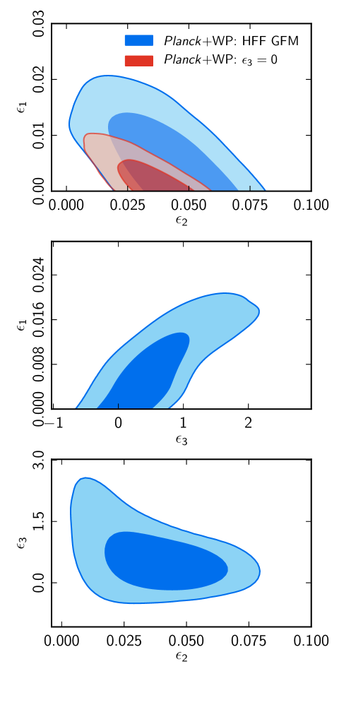
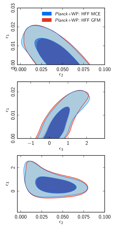
Sampling the power spectrum parameters , , and is not the only method for constraining slow-roll inflation. Another possibility is to sample the Hubble flow functions in the analytic expressions for the scalar and tensor power spectra (Stewart & Lyth, 1993; Gong & Stewart, 2001; Leach et al., 2002). In the Appendix, we compare the slow-roll inflationary predictions by sampling the HFF with Planck data and show that the results obtained in this way agree with those derived by sampling the power spectrum parameters. This confirms similar studies based on previous data (Hamann et al., 2008c; Finelli et al., 2010).
The spectral index estimated from Planck+WP data is
| (32) |
This tight bound on is crucial for constraining inflation. The Planck constraint on depends slightly on the pivot scales; we adopt Mpc-1 to quote our results, with at 95% CL. This bound improves on the most recent results, including the WMAP 9-year constraint of (Hinshaw et al., 2013), the WMAP 7-year + ACT limit of (Sievers et al., 2013), and the WMAP 7-year + SPT limit of (Story et al., 2013). The new bound from Planck is consistent with the theoretical limit from temperature anisotropies alone (Knox & Turner, 1994). When a possible tensor component is included, the spectral index from Planck+WP does not significantly change, with .
The Planck constraint on corresponds to an upper bound on the energy scale of inflation
| (33) |
at 95% CL. This is equivalent to an upper bound on the Hubble parameter during inflation of . In terms of slow-roll parameters, Planck+WP constraints imply at 95% CL, and .
| Model | Parameter | Planck+WP | Planck+WP+lensing | Planck + WP+high- | Planck+WP+BAO |
|---|---|---|---|---|---|
| CDM + tensor | |||||
| 0 | 0 | 0 | -0.31 |
The Planck results on and are robust to the addition of external data sets (see Table 4). When the high- CMB ACT + SPT data are added, we obtain and at 95% CL. Including the Planck lensing likelihood we obtain and , and adding BAO data gives and .
The above bounds are robust to small changes in the polarization likelihood at low multipoles. To test this robustness, instead of using the WMAP polarization likelihood, we impose a Gaussian prior to take into account small shifts due to uncertainties in residual foreground contamination or instrument systematic effects in the evaluation of , as performed in Appendix B of Planck Collaboration XVI (2014). We find at most a reduction of 8% for the upper bound on .
It is useful to plot the inflationary potentials in the plane using the first two slow-roll parameters evaluated at the pivot scale Mpc-1 (Dodelson et al., 1997). Given our ignorance of the details of the epoch of entropy generation, we assume that the number of e-folds to the end of inflation lies in the interval . This uncertainty is plotted for those potentials predicting an exit from inflation without changing the potential.
Figure 1 shows the Planck constraints in the plane and indicates the predictions of a number of representative inflationary potentials (see Lyth & Riotto (1999) for a review of particle physics models of inflation). The sensitivity of Planck data to high multipoles removes the degeneracy between and found using the WMAP data. Planck data favour models with a concave potential. As shown in Fig. 1, most of the joint 95% allowed region lies below the convex potential limit, and concave models with a red tilt in the range [0.945-0.98] are allowed by Planck at 95% CL. In the following we consider the status of several illustrative and commonly discussed inflationary potentials in light of the Planck observations.

Power law potential and chaotic inflation
The simplest class of inflationary models is characterized by a single monomial potential of the form
| (34) |
This class of potentials includes the simplest chaotic models, in which inflation starts from large values for the inflaton, . Inflation ends when slow-roll is no longer valid, and we assume this to occur at . According to Eqs. 5, 6, and 15, this class of potentials predicts to lowest order in slow-roll parameters , , . The model lies well outside the joint 99.7% CL region in the plane. This result confirms previous findings from, for example, Hinshaw et al. (2013), in which this model lies outside the 95% CL for the WMAP 9-year data and is further excluded by CMB data at smaller scales.
The model with a quadratic potential, (Linde, 1983), often considered the simplest example for inflation, now lies outside the joint 95% CL for the Planck+WP+high- data for -folds, as shown in Fig. 1.
A linear potential with (McAllister et al., 2010), motivated by axion monodromy, has and lies within the 95% CL region. Inflation with (Silverstein & Westphal, 2008), however, also motivated by axion monodromy, now lies on the boundary of the joint 95% CL region. More permissive entropy generation priors allowing could reconcile this model with the Planck data.
Exponential potential and power law inflation
Inflation with an exponential potential
| (35) |
is called power law inflation (Lucchin & Matarrese, 1985), because the exact solution for the scale factor is given by . This model is incomplete since inflation would not end without an additional mechanism to stop it. Under the assumption that such a mechanism exists and leaves predictions for cosmological perturbations unmodified, this class of models predicts and now lies outside the joint 99.7% CL contour.
Inverse power law potential
Intermediate inflationary models (Barrow, 1990; Muslimov, 1990) with inverse power law potentials
| (36) |
lead to inflation with , with and , where and . In intermediate inflation there is no natural end to inflation, but if the exit mechanism leaves the inflationary predictions for the cosmological perturbations unmodified, this class of models predicts and at lowest order in the slow-roll approximation (Barrow & Liddle, 1993).999See Starobinsky (2005) for the inflationary model producing an exactly scale-invariant power spectrum with beyond the slow-roll approximation. Intermediate inflationary models lie outside the joint 95% CL contour for any .
Hilltop models
In another interesting class of potentials, the inflaton rolls away from an unstable equilibrium as in the first new inflationary models (Albrecht & Steinhardt, 1982; Linde, 1982). We consider
| (37) |
where the ellipsis indicates higher order terms that are negligible during inflation but ensure positiveness of the potential later on. An exponent of is allowed only as a large field inflationary model, predicting and . This potential leads to predictions in agreement with Planck+WP+BAO joint 95% CL contours for super Planckian values of , i.e., .
Models with predict when . The hilltop potential with lies outside the joint 95% CL region for Planck+WP+BAO data. The case with is also in tension with Planck+WP+BAO, but allowed within the joint 95% CL region for when . For larger values of these models provide a better fit to the Planck+WP+BAO data. The hilltop model—without extra terms denoted by the ellipsis in Eq. (37)—is displayed in Fig. 1 in the standard range at different values of (this model approximates the linear potential for large ).
A simple symmetry breaking potential
The symmetry breaking potential (Olive, 1990)
| (38) |
can be considered as a self-consistent completion of the hilltop model with (although it has a different limiting large-field branch for non-zero ). This potential leads to predictions in agreement with Planck + WP + BAO joint 95% CL contours for super Planckian values of (i.e. .
Natural inflation
Another interesting class of potentials is natural inflation (Freese et al., 1990; Adams et al., 1993), initially motivated by its origin in symmetry breaking in an attempt to naturally give rise to the extremely flat potentials required for inflationary cosmology. In natural inflation the effective one-dimensional potential takes the form
| (39) |
where is a scale which determines the slope of the potential (see also Binétruy & Gaillard (1986) for an earlier motivation of a cosine potential for the inflaton in the context of superstring theory). Depending on the value of , the model falls into the large field () or small field () categories. Therefore, holds for small while , holds for large , approximating the potential in the latter case (with ). This model agrees with Planck+WP data for .
Hybrid inflation
In hybrid inflationary models a second field, , coupled to the inflaton, undergoes symmetry breaking. The simplest example of this class is
| (40) |
Over most of their parameter space, these models behave effectively as single-field models for the inflaton The second field is close to the origin during the slow-roll regime for , and inflation ends either by breakdown of slow roll for the inflaton at or by the waterfall transition of . The simplest models with
| (41) |
are disfavoured for most of the parameter space (Cortês & Liddle, 2009). Models with are disfavoured due to a high tensor-to-scalar ratio, and models with predict a spectral index , also disfavoured by the Planck data.
We discuss hybrid inflationary models predicting separately. As an example, the spontaneously broken SUSY model (Dvali et al., 1994)
| (42) |
predicts and . For and , is disfavoured by Planck+WP+BAO data at more than 95 CL. However, more permissive entropy generation priors allowing or a non-negligible give models consistent with the Planck data.
inflation
Inflationary models can also be accommodated within extended theories of gravity. These theories can be analysed either in the original (Jordan) frame or in the conformally-related Einstein frame with a Klein-Gordon scalar field. Due to the invariance of curvature and tensor perturbation power spectra with respect to this conformal transformation, we can use the same methodology described earlier.
The first inflationary model proposed was of this type and was based on higher order gravitational terms in the action (Starobinsky, 1980)
| (43) |
with the motivation to include semi-classical quantum effects. The predictions for inflation were first studied in Mukhanov & Chibisov (1981) and Starobinsky (1983), and can be summarized as and . Since is suppressed by another with respect to the scalar tilt, this model predicts a tiny amount of gravitational waves. This model predicts for and is fully consistent with the Planck constraints.
Non-minimally coupled inflaton
A non-minimal coupling of the inflaton to gravity with the action
| (44) |
leads to several interesting consequences, such as a lowering of the tensor-to-scalar ratio.
The case of a massless self-interacting inflaton () agrees with the Planck+WP data for . Within the range , this model is within the Planck+WP joint 95% CL region for , improving on previous bounds (Tsujikawa & Gumjudpai, 2004; Okada et al., 2010).
The amplitude of scalar perturbations is proportional to for , and therefore the problem of tiny values for the inflaton self-coupling can be alleviated (Spokoiny, 1984; Lucchin et al., 1986; Salopek et al., 1989; Fakir & Unruh, 1990). The regime is allowed and could be the Standard Model Higgs as proposed in Bezrukov & Shaposhnikov (2008) at the tree level (see Barvinsky et al. (2008); Bezrukov & Shaposhnikov (2009) for the inclusion of loop corrections). The Higgs case with has the same predictions as the model in terms of and as a function of . The entropy generation mechanism in the Higgs case can be more efficient than in the case and therefore predicts a slightly larger (Bezrukov & Gorbunov, 2012). This model is fully consistent with the Planck constraints.
4.3 Running spectral index
We have shown that the single parameter Harrison-Zeldovich spectrum does not fit the data and that at least the first two terms and in the expansion of the primordial power spectrum in powers of given in Eq. 10 are needed. Here we consider whether the data require the next term known as the running of the spectral index (Kosowsky & Turner, 1995), defined as the derivative of the spectral index with respect to , for scalar or tensor fluctuations. If the slow-roll approximation holds and the inflaton has reached its attractor solution, and are related to the potential slow-roll parameters, as in Eqs. 17 and 18. In slow-roll single-field inflation, the running is second order in the Hubble slow-roll parameters, for scalar and for tensor perturbations (Kosowsky & Turner, 1995; Leach et al., 2002), and thus is typically suppressed with respect to and , which are first order. Given the tight constraints on the first two slow-roll parameters and ( and ) from the present data, typical values of the running to which Planck is sensitive (Pahud et al., 2007) would generically be dominated by the contribution from the third derivative of the potential, encoded in (or ).
While it is easy to see that the running is invariant under a change in pivot scale, the same does not hold for the spectral index and the amplitude of the primordial power spectrum. It is convenient to choose such that and are uncorrelated (Cortês et al., 2007). This approach minimizes the inferred variance of and facilitates comparison with constraints on in the power law models. Note, however, that the decorrelation pivot scale depends on both the model and the data set used.
| Model | Parameter | Planck+WP | Planck+WP+lensing | Planck+WP+high- | Planck+WP+BAO |
|---|---|---|---|---|---|
| CDM + | |||||
| -1.50 | -0.77 | -2.95 | -1.45 | ||
| + | |||||
| CDM + | |||||
| -2.65 | -2.14 | -5.42 | -2.40 | ||
| CDM + + | |||||
| -1.53 | -0.26 | -3.25 | -1.5 |
We consider a model parameterizing the power spectrum using and , where . The joint constraints on and at the decorrelation scale of Mpc-1 are shown in Fig. 2. The Planck+WP constraints on the running do not change significantly when complementary data sets such as Planck lensing, CMB high- and BAO data are included. We find
| (45) |
which is negative at the 1.5 level. This reduces the uncertainty compared to previous CMB results. Error bars are reduced by 60% compared to the WMAP 9-year results (Hinshaw et al., 2013), and by 20–30% compared to WMAP supplemented by SPT and ACT data (Hou et al., 2012; Sievers et al., 2013). Planck finds a smaller scalar running than SPT + WMAP7 (Hou et al., 2012), and larger than ACT + WMAP7 (Sievers et al., 2013). The best fit likelihood improves by only ( when high- data are included) with respect to the minimal case in which is scale independent, indicating that the deviation from scale independence is not very significant. The constraint for the spectral index in this case is at 68% CL at the decorrelation pivot scale Mpc-1. This result implies that the third derivative of the potential is small, i.e., , but compatible with zero at 95% CL, for inflation at low energy (i.e., with ).

We also test the possibility that the running depends on the wavelength so that is nonzero. With Planck+WP data, we find . This result is stable with respect to the addition of complementary data sets, as can be seen from Table 5 and Fig. 3. When is allowed in the fit, we find a value for the running consistent with zero.
Finally we allow a non-zero primordial gravitational wave spectrum together with the running. The tensor spectral index and its running are set by the slow-roll consistency relations to second order, with and . Planck measures the running to be when tensors are included (see Table 5 and Fig. 4). The constraints on the tensor-to-scalar ratio are relaxed compared to the case with no running, due to an anti-correlation between and , as shown in Fig. 4 for Planck+WP+BAO.
Varying both tensors and running, Planck+WP implications for slow-roll parameters are at 95% CL, , and .
In summary, the Planck data prefer a negative running for the scalar spectral index of order but at only the 1.5 significance level. This is for Planck alone and in combination with other astrophysical data sets. Weak statistical evidence for negative values of has been claimed in several previous investigations with the WMAP data and smaller scale CMB data (e.g., Spergel et al., 2003; Peiris et al., 2003; Dunkley et al., 2011; Hinshaw et al., 2013; Hou et al., 2012).
If primordial, negative values for of order would be interesting for the physics of inflation. The running of the scalar spectral index is a key prediction for inflationary models. It is strictly zero for power law inflation, whose fit to Planck was shown to be quite poor in the previous section. Chaotic monomial models with predict , and the same order of magnitude is quite typical for many slow-roll inflationary models, such as natural inflation (Adams et al., 1993) or hilltop inflation (Boubekeur & Lyth, 2005). It was pointed out that a large negative running of would make it difficult to support the -foldings required from inflation (Easther & Peiris, 2006), but this holds only without nonzero derivatives higher than the third order in the inflationary potential. Designing inflationary models that predict a negative running of with an acceptable and number of -folds is not impossible, as the case with modulated oscillations in the inflationary potential demonstrates (Kobayashi & Takahashi, 2011). This occurs, for instance, in the axion monodromy model when the instanton contribution is taken into account (McAllister et al., 2010), giving the potential
| (46) |


4.4 Open inflation
Most models of inflation predict a nearly flat spatial geometry with small deviations from perfect spatial flatness of . Curvature fluctuations may be regarded as local fluctuations in the spatial curvature, and even in models of inflation where the perturbations are calculated about a spatially flat background, the spatial curvature on the largest scales accessible to observation now are subject to fluctuations from perfect spatial flatness (i.e., ). This prediction for this fluctuation is calculated by simply extrapolating the power law spectrum to the largest scale accessible today, so that as probed by the CMB roughly represents the local curvature fluctuation averaged over our (causal) horizon volume. Although it has sometimes been claimed that spatial flatness is a firm prediction of inflation, it was realized early on that spatial flatness is not an inexorable consequence of inflation and large amounts of spatial curvature (i.e., large compared to the above prediction) can be introduced in a precise way while retaining all the advantages of inflation (Gott, 1982; Gott & Statler, 1984) through bubble nucleation by false vacuum decay (Coleman & De Luccia, 1980). This proposal gained credence when it was shown how to calculate the perturbations in this model around and beyond the curvature scale (Bucher et al., 1995; Bucher & Turok, 1995; Yamamoto et al., 1995; Tanaka & Sasaki, 1994). See also Ratra & Peebles (1995, 1994) and Lyth & Stewart (1990). For more refined later calculations see for example Garriga et al. (1998, 1999), Gratton & Turok (1999), and references therein. For predictions of the tensor perturbations see for example Bucher & Cohn (1997), Sasaki et al. (1997), and Hertog & Turok (2000).
An interesting proposal using singular instantons and not requiring a false vacuum may be found in Hawking & Turok (1998), and for calculations of the resulting perturbation spectra see Hertog & Turok (2000) and Gratton et al. (2000). Models of this sort have been studied more recently in the context of the string landscape. (See, for example, Vilenkin (2007) for a nice review.) Although some proposals for universes with positive curvature within the framework of inflation have been put forth (Gratton et al., 2002), it is much harder to obtain a closed universe with a spatial geometry of positive spatial curvature (i.e., ) (Linde, 2003).
Theoretically, it is of interest to measure to an accuracy of approximately or slightly better to test the prediction of simple flat inflation for this observable. A statistically significant positive value would suggest that open inflation, perhaps in the context of the landscape, was at play. A statistically significant negative value could pose difficulties for the inflationary paradigm. For a recent discussion of these questions, see for example Freivogel et al. (2006), Kleban & Schillo (2012), and Guth & Nomura (2012).

In order to see how much spatial curvature is allowed, we
consider a rather general model including the parameters
and as well as .
We find that
with Planck+WP, and
with Planck+WP+BAO.
More details can be found by consulting the parameter tables available
online.101010Available at: http://www.sciops.esa.int/index.php
?project=planck&page=Planck_Legacy_Archive
Figure 5 shows
and for this family of models.
We conclude that any possible spatial curvature is small in magnitude
even within this general model and that the spatial curvature scale is
constrained to lie far beyond the horizon today.
Open models predict a tensor spectrum enhanced at small wavenumber , where corresponds to the curvature scale, but
our constraint on and cosmic variance imply that
this aspect is likely unobservable.
4.5 Relaxing the assumption of the late-time cosmological concordance model
The joint constraints on and shown in Fig. 1 are one of the central results of this paper. However, they are derived assuming the standard CDM cosmology at late times (i.e., ). It is therefore natural to ask how robust our conclusions are to changes of the late time cosmological model. We discuss two classes of models: firstly, changes to the CDM energy content; and secondly, a more general reionization model. These extensions can lead to degeneracies of the additional parameters with or .111111 We considered a further generalization, which also causes the joint constraints on and to change slightly. We allowed the amplitude of the lensing contribution to the temperature power spectrum to vary as a free parameter. In this case we find the following Planck+WP+BAO constraints: , at 95% CL.
4.5.1 Extensions to the energy content
We consider the CDM++, CDM++, CDM++ and CDM++ extensions of the standard model. This selection is motivated by the impact on the CMB damping tail of the first two and the effect on the Sachs-Wolfe plateau at low multipoles for the latter two. The resulting contours are shown in Fig. 6. While the lower limit on is stable under all extensions considered here, the models that alter the high- part of the spectrum permit significantly bluer spectral tilts, and accordingly also lead to a weaker bound on the tensor-to-scalar ratio. By allowing to float, we obtain and at 95% CL.121212Selected non-standard values for deserve further investigation. For the additional fractional contribution motivated by a Goldstone boson (Weinberg, 2013), we obtain and at 95% CL for Planck+WP+BAO+high-. For an additional species of neutrinos, we obtain and at 95% CL for Planck+WP+BAO+high-. For CDM++ we obtain and at 95% CL. The models modifying the large-scale part of the power spectrum, on the other hand, do not lead to a notable degradation of constraints on either or ( and at 95% CL for CDM++, and and at 95% CL for CDM++).

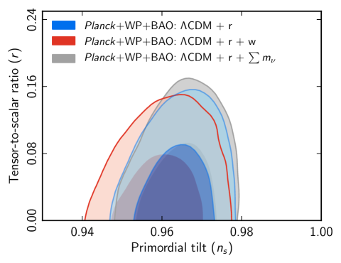
4.5.2 General reionization scenario
In the standard rapid reionization scenario typically used in CMB analysis, the Universe is assumed to be completely transparent after recombination, but the ionization fraction increases from zero to one over a duration at a certain redshift which is the only unknown parameter of the reionization model. This model is obviously simplistic, but for CMB analysis it works quite well because the CMB has little sensitivity to the details of how the ionization fraction changes from 0 to 1. In this section we study to what extent allowing more general reionization scenarios may alter some of the conclusions concerning the constraints on and as well as on . As discussed in Mortonson & Hu (2008a) and Mortonson & Hu (2008b), CMB anisotropies constrain reionization almost entirely by using the shape of the large-scale EE power spectrum, and the power is redistributed from larger to smaller scales for reionization processes which take place during a non-negligible redshift interval, since they start at an earlier epoch.
We use the method developed by Mortonson & Hu (2008a) to describe and constrain the reionization history. A complete principal component basis serves to describe the effect of reionization on the large-scale -mode polarization power spectrum. Following Mortonson & Hu (2008a) we bin the ionization history using equal width bins with ranging from to . For the redshifts we assume values for which take into account first (and possibly second) helium ionization and complete hydrogen ionization ( for and for ). For we fix as the value of expected before reionization (and after primordial recombination). Any reionization history can be parameterized as a free function of redshift by decomposing the ionization fraction as , where the principal components, , are the eigenfunctions of the Fisher matrix computed by taking the derivatives of the EE polarization power spectrum with respect to and is a fiducial ionization fraction. Following Mortonson & Hu (2008a) we consider here the first five eigenfunctions, with , which will be varied with the other cosmological parameters.
In Fig. 7 we plot the 68% and 95% CL regions for and The constraint on the tensor-to-scalar ratio is not significantly affected by this additional marginalization, increasing to at 95% CL. The scalar spectral index is increased to , compared with obtained with the rapid reionization scheme. This is the same trend as noted in Pandolfi et al. (2010) using WMAP data, but the effect is less significant due to the improved measurement of the temperature spectrum by Planck. The larger freedom in the reionization history increases the width of the posterior on the derived optical depth, which is still partially degenerate with the scalar spectral index of primordial perturbations. The model is still excluded at high significance; however, we find compared to the CDM model.

5 Inflationary model comparison
In Sect. 4.2 several representative families of parameterized models for the inflationary potential were analysed within the slow-roll approximation in the neighbourhood of the pivot scale . Approximate constraints were applied to reject models for which there is no plausible scenario for entropy generation. In this section we revisit some of the parametric models defined in Sect. 4.2. Here, however, the modes for the first order perturbations, as described in Sect. 2.2, are integrated numerically. Thus there is no slow-roll approximation, and the issue of the existence of a plausible scenario for entropy generation is examined more carefully. We perform a statistical model comparison between the competing parameterized potentials, both within the framework of Bayesian model comparison and in terms of the relative likelihoods of the best fit models from each parameterized family.
As noted in Sect. 2.3, considerable uncertainty surrounds what occurred during the epoch of entropy generation, particularly with respect to the energy scale at which entropy generation ends and the average equation of state between that epoch and the end of inflation. For this reason, we explore a number of scenarios for this intermediate era during which entropy generation takes place. The models compared in this section include inflation with power law potentials, defined in Eq. 34, with several representative values for ; natural inflation, in Eq. 39; and hilltop inflation, with and in Eq. 37.
The free parameters in these inflationary potentials may vary over several orders of magnitude corresponding to unknown scales in high energy particle physics. Consequently a logarithmic prior is a sensible choice for these parameters. However, there is no theoretical guidance on how to truncate these model priors. We therefore adopt broad priors initially and then truncate them as follows in order to compare all the models on an equal footing.
The strongest constraint on the inflationary parameter space comes from the amplitude of the primordial power spectrum. This is a free parameter in most models, and successful structure formation in a universe dominated by cold dark matter has long been known to require primordial fluctuations with , or (see e.g., Zeldovich, 1972; Linde, 1990). We can therefore immediately reject models for which is far from this value, so regions of parameter space which do not yield are a priori excluded. This range is generous relative to estimates of prior to Planck (e.g., Komatsu et al., 2011), but the results do not depend strongly on the range chosen. This effectively truncates the logarithmic priors on the model parameters, leaving a parameter subspace compatible with basic structure formation requirements.
For the single parameter models this requirement defines the range of in Eq. 34. However, for generic multi-parameter models, an -based cut may select a nontrival region of parameter space, as happens for the two cases considered here (see e.g., Fig. 1 in Easther & Peiris (2012)). Without the -based cut in the prior, the parameter volume for both natural and hilltop inflation would be rectangular, and the corresponding Bayesian evidence values computed for these models would be lowered.
| Model | Priors |
|---|---|
| Natural | |
| Hilltop | |
| CDM | |
| Matching | Prior |
As discussed in Sect. 2.3, specifying an inflationary potential does not enable us to predict the late time CMB angular power spectra. The subsequent expansion history and details of the epoch of entropy generation are required to relate the value of the inflaton field at Hubble radius crossing to comoving wavenumbers in today’s Universe, through Eq. 24. Physically, the fundamental parameter that sets the observable perturbation spectrum is the value of the field at which the pivot mode leaves the Hubble radius. It can be rescaled by a shift , and the range over which changes during inflation varies greatly between models. Consequently we treat the remaining number of -folds, , after the pivot scale leaves the Hubble radius as a free parameter with a wide uniform prior, since this quantity has a consistent interpretation across models. The pivot scale used to compute is Mpc-1. However, given our ignorance concerning the epoch of entropy generation, a multitude of entropy generation scenarios for each inflationary potential can occur. Some possibilities are as follows, with parameters referring to Eq. 24.
-
1.
Instantaneous entropy generation scenario. At the end of inflation, all the energy in the inflaton field is instantaneously converted into radiation.
-
2.
Restrictive entropy generation scenario (narrow range for ). GeV, and
-
3.
Permissive entropy generation scenario (wide range for ). GeV, and
The equations of state with in the range appear less plausible, but models with these values have been put forward (Pallis, 2006), so this possibility cannot be completely excluded. Moreover the parameterization captures a variety of scenarios in which the post-inflationary Universe is thermalized, but not radiation dominated, including phases of coherent oscillations (Martin & Ringeval, 2010; Easther et al., 2011), resonance (Traschen & Brandenberger, 1990; Kofman et al., 1994, 1997; Allahverdi et al., 2010), kination (Spokoiny, 1993; Chung et al., 2007), secondary or thermal inflation (Lyth & Stewart, 1996), moduli domination (Banks et al., 1994; de Carlos et al., 1993), primordial black hole domination (Anantua et al., 2009), or a frustrated cosmic string network (Burgess et al., 2005), all of which lead to an expansion rate differing from that of a radiation dominated universe.
| Model | Instantaneous | Restrictive | Permissive | |||
|---|---|---|---|---|---|---|
| entropy generation | entropy generation | entropy generation | ||||
| Natural | ||||||
| Hilltop | ||||||
| CDM | ||||||
At the other extreme, the decision to exclude as done here, is not completely justifiable. We cannot, for example, rule out a first order phase transition at a lower energy scale that would drive below , but here we neglect this possibility. Our analysis does not preclude a secondary period of inflation, but does require that the average expansion during the post-inflationary regime parameterized by should not be inflationary. This caveat should be kept in mind.
For some of the parameterized models, tighter constraints can, in principle, be placed on . It has been argued (see e.g., Liddle & Leach, 2003) that for the potential, the uncertainties concerning entropy generation contribute almost no uncertainty in the determination of . This is because according to the virial theorem, a field sloshing about in a quartic potential has the same average , namely , as the radiation equation of state. More generally, for a potential of the form around the minimum, (Turner, 1983); therefore, one may argue that should be restricted to the interval whose endpoints are and . This approach was taken by Martin & Ringeval (2010) in obtaining Bayesian constraints on the reheating temperature for monomial potentials from the CMB. However this scenario requires a carefully tuned potential that has approximately a shape, both at large field values and near the origin far below the inflationary scale. Typically, potentials for which at large field values can have very different shapes near the origin. Thus, following Easther & Peiris (2012), in this paper we explore a broader range of for these models (including the cases above as subsets) in order to obtain data-driven constraints on .
In this paper we focus on the three representative scenarios itemized above, referred to hereafter as scenarios (1), (2), and (3). Our algorithm draws a value of and then given the value of , computes , which is a derived parameter. Models for which lies outside the specified range of each scenario under consideration are excluded.
The full set of priors for the inflationary physics is given in Table 6. Dimensionful quantities are expressed in units with reduced Planck mass set to unity.
Due to the nontrivial likelihood surfaces and the large dimensionality of the parameter spaces explored in this section, we use ModeCode coupled to MultiNest v3.0131313Made available ahead of public release to the Planck Collaboration by Farhan Feroz and Mike Hobson (Feroz et al., 2013). to map out the parameter space. In addition to the standard nested sampling (NS) algorithm, MultiNest v3.0 enables nested importance sampling (NIS), resulting in substantial speed gains141414We have carried out extensive tests of NIS versus NS, and chosen the following settings for the computations presented here: NIS on, constant efficiency mode on, live points, tolerance and efficiency parameters set to and , respectively. and significant enhancements in the accuracy of the Bayesian evidence computation compared to NS alone for the same computational setup.
5.1 Results
Table 7 presents model comparison results for the ensemble of parameterized potential families described above. We report the Bayesian evidence (model averaged likelihood) ratio, which provides a self-consistent framework for calculating the betting odds between models (see Sect. 3.4). The uncertainty in these logarithmic evidence values is approximately . We also report the values computed from the values found by the sampler.
The monomial models have a single parameter potential, and the natural and hilltop inflation models have two parameters each. All entropy generation scenarios except case (1) contribute one additional parameter to the inflationary sector. The evidence ratios and values are presented with respect to the CDM cosmological model.
None of the inflationary models tested here fit the data as well as the CDM model. This mostly reflects that there is no evidence in the data for different from zero. Furthermore, the priors listed in Table 6 for the CDM primordial sector are purely phenomenological, roughly corresponding to ranges somewhat broader than WMAP constraints. Narrowing them around the best fit model arbitrarily increases the evidence in its favour. Instead it is instructive to compare the relative evidence for the inflationary models presented.
Table 7 shows that the model is decisively ruled out by Planck, confirming previous analyses by the WMAP team (Peiris et al., 2003; Spergel et al., 2007; Dunkley et al., 2009; Komatsu et al., 2011) based on the model track plotted on the plane. Recent model selection analyses (Martin et al., 2011; Easther & Peiris, 2012) with WMAP 7-year data found that the model was already disfavoured by odds of about : against. With Planck, the odds against this model are at least : compared to CDM for a broad range of entropy generation scenarios. The same conclusion is confirmed by the extremely poor values for the model. Given the strength of our results, in the flexible setting of the permissive entropy generation scenario, it is possible not just to rule out models where the potential is of the quartic form in the full range from the origin to the inflationary scales, but also a general class where the potential is of the form in the -range where the cosmological perturbations are generated, but exhibits a different shape near the origin.
Two other large field models, the quadratic potential and natural inflation, are somewhat disfavoured by the Planck data, especially when broader entropy generation scenarios are considered. Compared with the CDM model, these models are disfavoured by – depending on the entropy generation scenario. This reflects the analysis of Sect. 4, where the overlap of the model predictions and the data constraints on the plane is seen to be mostly outside the joint % CL contour. However, from the Bayesian evidence point of view, it is too early to declare these models incompatible with the data. To make this judgement, it is more prudent to compare these models to the case, which has the best evidence with respect to CDM, rather than to CDM itself, which provides our reference point for the evidence calculation, but has arbitrary prior ranges. In their simplest forms—instantaneous entropy generation—the and natural inflation models are only disfavoured by odds of about –: against, which does not rise to a high level of significance.151515In comparison, odds of : are considered highly significant in this context.
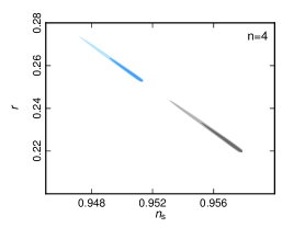

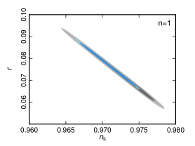
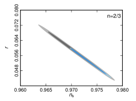


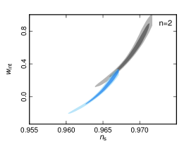
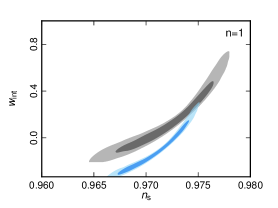


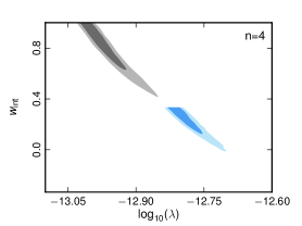
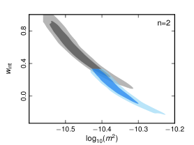
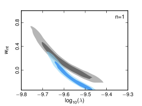

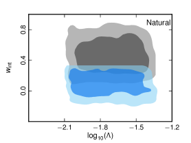
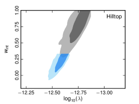


The models most compatible with the Planck data in the set considered here are the two interesting axion monodromy potentials, (McAllister et al., 2010) and (Silverstein & Westphal, 2008), which are motivated by inflationary model building in the context of string theory. The hilltop model presents an interesting case. This model was previously found to be compatible with WMAP 7-year data, performing almost as well as the monodromy potentials (Easther & Peiris, 2012). However it exhibits significant tension with the Planck data, both in terms of evidence ratios and the maximum likelihood. The only exception is the entropy generation scenario (3) which has odds of greater than : against compared to CDM, and yet the maximum likelihood is not significantly different from the case. This indicates that while the extra freedom allowed by the least restrictive entropy generation scenario improves the best fit, this prior is not very predictive of the data. However, the result seems counterintuitive and merits further comment; we will consider this question further at the end of this section when parameter estimation results are discussed.
We now turn to parameter constraints. Figure 8 presents marginalized joint constraints from Planck+WP alone on the derived parameters and Figure 9 shows the corresponding joint constraints on and , again a derived parameter. Figure 10 shows joint constraints on and the potential parameter ( in the case of natural inflation). It is instructive to consider the three sets of figures together. The restrictive and permissive entropy generation scenarios are shown on all panels; the instantaneous entropy generation case is shown for the two parameter models, natural inflation and hilltop, in Fig. 8—for the monomial potentials this case corresponds to the lowest- extremity of the restrictive case constraints, and to in the other two figures.
The quartic potential conflicts with the data because it predicts a high tensor-to-scalar ratio. Hence the model maximizes its likelihood by pushing towards the lower-, bluer- limits of its parameter space, which corresponds to increasing as much as allowed by the entropy generation prior. The contours terminate at the lowest- limit when each entropy generation case hits its prior upper limit (i.e., and for restrictive and permissive entropy generation, respectively). For each case, the lower limit on , corresponding to the reddest- extremity of the confidence contours, is data-driven. The quadratic potential encounters the same difficulty but at a less extreme level.
The two axion monodromy potentials are compatible with a wide range of entropy generation scenarios. The instantaneous entropy generation scenario is compatible with the data for both models. For restrictive entropy generation in the model, we obtain a data-driven upper limit on , which just touches the case at the 95% CL. At the lower limit, the posterior is truncated by the prior, as for the case. For the latter, there is a data-driven upper limit on which is controlled by the upper limit on . For permissive entropy generation, the upper and lower limits on for both models are data-driven, corresponding to the upper and lower limits on respectively.
The constraints on natural inflation require some interpretation. The relationship between the empirical and parameters and the potential parameters for natural inflation is discussed in detail by Savage et al. (2006) and Mortonson et al. (2011) along with parameter constraints derived from WMAP 3-year (Spergel et al., 2007) and WMAP 7-year (Larson et al., 2011), respectively. In this model, there is a degeneracy between and in the limit where these parameters are large so that natural inflation resembles the quadratic model. The priors are chosen to exclude most of this region. The priors on and still allow a region of nearly degenerate models that contribute to a ridge seen in the natural inflation panel of Fig. 8. These models closely match the values of and seen in the quadratic potential constraints. The marginalized constraints on and depend strongly on the prior on due to the projection of a large number of degenerate models onto this ridge. Therefore the apparent preference for this region of parameter space over models with lower values of is largely due to this effect and is not driven by the data. This highly nonlinear mapping between the logarithmic priors on the potential parameters and the power law parameters (which are derived parameters in this analysis) leads to a strong projection effect, which accounts for the difference in visual appearance between these contours and the region labelled natural inflation in Fig. 1.
Generally, for fixed , decreasing and reduces both and . Thus natural inflation models can have lower values of than the quadratic potential without increasing and . This feature means that the potential parameters for this model are relatively uncorrelated with , in contrast with the other models considered here, as illustrated in the Fig. 10. Nevertheless we obtain data-driven bounds on in the permissive entropy generation case as well as a lower bound in the restrictive entropy generation case. Both bounds overlap with the instantaneous generation limit.
The upper panel of Fig. 11 shows our lower limit of (95% CL), compared with the WMAP7 limit (95% CL) reported by Mortonson et al. (2011). Indeed, the Planck limit is in agreement with the Planck prediction presented in that work. There is a hint of an upper limit on as well, driven by the fact that this corresponds to the quadratic inflation limit, which is in tension with the data. However this is only a effect.
The hilltop model has two distinct branches: a small-field scenario, where and ; and a large-field limit in which (Adshead et al., 2011). Physically, the small-field limit is consistent with the Lyth bound, and we can select it by fixing in the prior. We observe that the data select out this small field branch, which requires explanation given that we know that the model (the limit of the large field branch) is perfectly compatible with the data. In fact, this can be tested by restricting the prior by hand to the large-field branch. The hilltop model constitutes a difficult sampling problem, as is apparent from Fig. 4 in Easther & Peiris (2012). An examination of the progress of the nested sampler for the case of the full hilltop prior reveals the reason for the small-field branch being selected out. In this case, the posterior for the large-field branch is extremely thin compared to the model prior in this regime—much thinner than the posterior for the small-field branch in comparison to its respective prior. Therefore this region occupies very little probability mass, and is dropped in preference to the more predictive small-field branch. This high likelihood but extremely thin ridge is also responsible for the counterintuitive result reported in the model selection analysis, where the model was found to have a good with respect to CDM, and yet be highly disfavoured by the Bayesian evidence. In summary, confirming the results of Sect. 4, this model is in agreement with the data in the limit where it overlaps the linear model. But since this region of high likelihood occupies a very small fraction of the prior, this model is heavily penalized by the Bayesian evidence for failing to predict the data over most of its prior space.
6 Observable window of inflation
Section 4.2 presented an analysis of several representative inflationary potentials within the framework of the slow-roll approximation and their compatibility with the Planck data. The results are summarized in Fig. 1. In that case the full potential is considered in order to identify a plausible range for the location of on the potential This requires a complete story. In other words, the potential must be specified starting above the point where the largest observable scales first exited the Hubble radius, and extending to the minimum of the potential.
In this section we explore another approach. We adopt the point of view that we are interested in reconstructing the inflationary potential only over the observable range—that is, the interval of corresponding to the scales observable today in the CMB. We constrain the potential over the range where these scales exited the Hubble radius during inflation as well as a few -folds before and after. The cosmological perturbations are not imprinted instantaneously at the moment of Hubble radius crossing, but rather gradually over a few -folds. We expand around , taking the view that a plausible extension of the potential outside this observable range is always possible, so that one has precisely the number of -folds of inflation needed for to correspond to today.
The argument is that one can always end inflation abruptly by imposing a sharp waterfall feature where needed, or prolong inflation by inserting a sufficiently long plateau into the potential by hand, for example, for models with a large tilt. A foreseeable objection to this approach is that the extensions of the potential required outside the observable window may render the potential unnatural. This possibility should be kept in mind, although naturalness is an elusive and uncomfortably subjective concept. The analysis in this section does not rely on the slow-roll approximation. Instead each mode is integrated exactly by numerical integration, as described in Sect. 2.2, under the assumption of a canonical kinetic term.
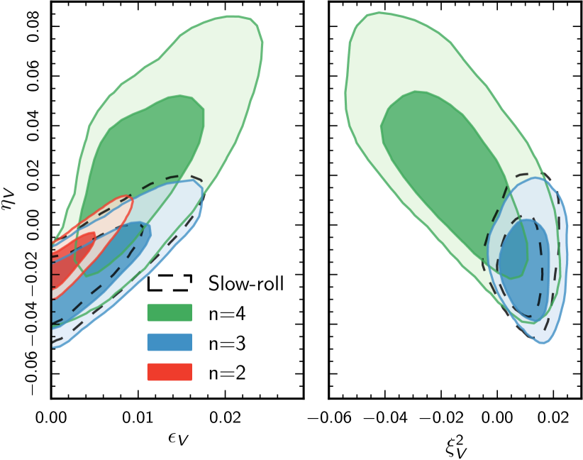
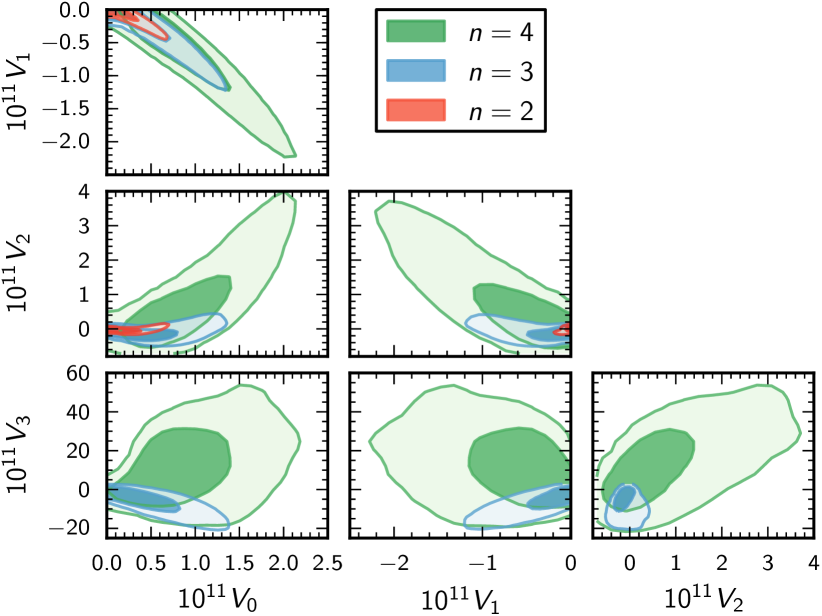
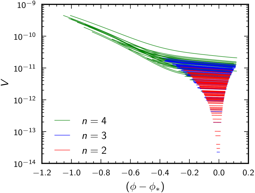
Two complementary approaches to reconstruct the potential have been explored in the literature. The first approach, followed in this paper, expands the potential directly in powers of In this case the numerical integration of the slow-roll solution must start sufficiently early so that any initial transient has had a chance to decay, and one is in the attractor solution when the dynamics of the largest observable modes in the Universe today start to have an interesting evolution. This is the approach followed, e.g., by Lesgourgues & Valkenburg (2007) and Mortonson et al. (2011) using publicly available codes.161616http://wwwlapp.in2p3.fr/valkenbu/inflationH/, http://zuserver2.star.ucl.ac.uk/~hiranya/ModeCode/.
A second approach expands as a Taylor series in As discussed in Sect. 2.2, this has the advantage that determines both the potential and the solution so the issue of having to start sufficiently early in order to allow the initial transient to decay is avoided. This method was used, for example, in Kinney (2002), Kinney et al. (2006), Peiris & Easther (2006a), Easther & Peiris (2006), Peiris & Easther (2006b), and Peiris & Easther (2008) using analytic and semi-analytic approximations, and in Lesgourgues et al. (2008), Powell & Kinney (2007), Hamann et al. (2008c), and Norena et al. (2012) using a fully numerical approach.
These approaches could lead to results that differ from those in Sect. 4.2. Firstly, if the running of the index is large, the slow-roll approximation taken to second order is not necessarily accurate for all models allowed by the data. The relation between the spectral parameters (, , , ) and the underlying inflationary potential is therefore uncertain. Secondly, for spectra with a large running, there is no guarantee that an inflationary model giving such a spectrum exists. All allowed models have , so these models are consistent with at the pivot scale. However, towards the edge of the observable range, the potential may become incompatible with (i.e., with the requirement of inflationary expansion). These possible pitfalls are avoided using the methods in this section, since the data have been fit directly by the candidate or , computed numerically without any slow roll assumptions over the entire observable range.
| from | from | |||
| 2 | 3 | 4 | slow-roll | |
| – | ||||
| – | – | – | ||
| 0 | ||||
| from | |||
|---|---|---|---|
| 2 | 3 | 4 | |
We define a class of models over the observable range based on the expectation that the potential should be smooth. is approximated by a Taylor expansion up to order and we explore the cases and For each , we integrate over inflationary fluctuations using the inflation module implemented in CLASS171717http://class-code.net (Lesgourgues, 2011; Blas et al., 2011) as described in Lesgourgues & Valkenburg (2007). Potentials are rejected for which the attractor solution cannot be reached when the largest observable scales cross the Hubble radius. The parameters sampled are the potential and its derivatives at the pivot scale when crosses the Hubble radius during inflation.
To avoid parameter degeneracies, we impose uniform priors on and at the pivot field value The advantage of uniform priors on these parameters is that—to the extent that the slow-roll conditions are satisfied—these coefficients relate linearly to observable quantities such as , , and . Figure 12 and Table 8 show the posterior probability for these coefficients, and Fig. 13 shows the posterior probability for the Taylor series coefficients . In Fig. 14, we show the observable range of the best fitting inflaton potentials (for a sample extracted randomly from the converged Markov chains). The edges of the observable range correspond to Hubble crossing for the minimum and maximum values of used in the Boltzmann code. We stress here that the Planck data suggest a flat potential when the lowest order slow-roll primordial spectra are considered, as analysed in Sect. 4.2. However, when the restrictions to lowest order in the slow-roll approximation are relaxed, the inflaton potential can differ markedly from a plateau-like potential, as the green curves in Fig. 14 show.
When fitting for each model in parameter space, we compute (, , , and ) at the pivot scale a posteriori directly from the numerical primordial spectra. The results are shown in Table 9 and can be compared to those of Table 5 in Sect. 4. We can also use the results of Sect. 4 for the CDM++ model to infer the potential parameters (, , and ) using the second-order slow-roll expressions, and compare different approaches in the space of potential parameters (see Fig. 12 and the last column in Table 8).
The model with a quadratic potential in the observable window () leads to bounds on , , , and very close to the CDM+ case. This is not a surprise since such potentials cannot give values of and compatible with the data and at the same time a large running. A significant can be generated only in the presence of a large (i.e., with a significant ). Since quadratic potentials produce little running, they are faithfully described by the slow-roll approximation.
The model with a cubic term () has the freedom to generate a large running, . Indeed one can check that the results for the model are close to those of the CDM++ model presented in Sect. 4. The agreement between these two models remains very good, despite the fact that in the presence of a large running, the slow-roll approximation can become inaccurate. The running in a potential with is not exactly scale invariant; this is not captured by the CDM++ parameterization.
The model has even more freedom, allowing a considerable running of the running (to the extent that inflation holds during the observable -folds). In that case, the spectrum is better fitted when the two parameters and are non-zero. In Fig. 14, we see that most potentials have a long and steep tail for , with a kink around (in natural units). This shape generates a significant running on the largest observable scales, while preserving a smaller running on smaller scales. With such a feature in the scalar primordial spectrum at large scales combined with a non-zero contribution from tensor fluctuations, the best fit model for has a temperature spectrum very close to that of the minimal CDM model for , but not for smaller multipoles. The amplitude of the Sachs-Wolfe plateau is smaller. This allows the large-scale data points from Planck to be fitted slightly better. However, the case still lies at the edge of the 95% CL, and the minimum effective of this model is smaller than in the case by only 3.7.
A comparison of the and results clearly shows that the process of expanding the inflaton potential to various orders and fitting it to the data does not converge (at least not by ). Given the – preference of Planck data for a nonzero running and running of the running, we find that a model-independent reconstruction of the inflaton potential is not possible under the assumptions of this section. In other words, as long as we assume that can be described during and after observable inflation by a polynomial of order 2 or 3, we can put strong bounds on and . But if we introduce more derivatives to describe the observable part of the potential and allow complete freedom to extrapolate outside this region, the constraints can be easily evaded.
7 Primordial power spectrum reconstruction
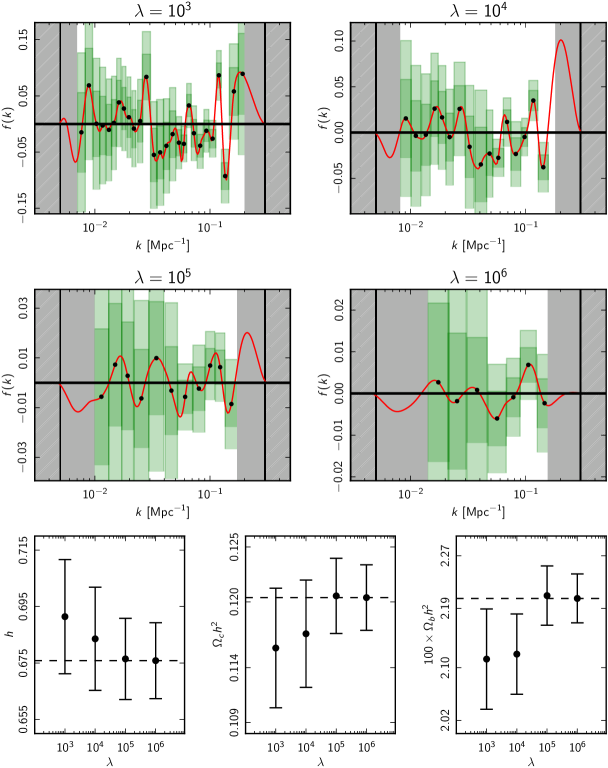
In this section we report on a search for features in the primordial power spectrum. In the basic six parameter model studied in the companion Planck paper Planck Collaboration XVI (2014), the primordial power spectrum , which includes only the adiabatic mode, is modelled using the power law , for which the best fit values are and for a pivot scale . An extension of this parameterization is also considered allowing for a running of the spectral index (). But in all cases considered it was assumed that the power spectrum is smooth and without bumps, sharp features, or wiggles. In this section we investigate whether any statistically significant evidence for features is present in the data when these assumptions are relaxed. Allowing an arbitrary function for the input power spectrum is not an option because in this case the recovered primordial power spectrum is dominated by small-scale noise. Instead we consider here a penalized likelihood approach where a preference for smooth power spectra is imposed. Section 8 of this paper pursues a complementary approach where several parametric models for wiggles and features are explored to see whether a statistically significantly better fit can be obtained.
An extensive literature exists on how to search for features in the power spectrum using a wide range of methods. The following papers and the references therein provide a sampling of the literature on non-parametric reconstruction: Richardson-Lucy deconvolution (Lucy, 1974; Richardson, 1972; Hamann et al., 2010; Shafieloo & Souradeep, 2004, 2008), deconvolution (Tocchini-Valentini et al., 2005, 2006; Ichiki & Nagata, 2009; Nagata & Yokoyama, 2008, 2009), smoothing splines (Verde & Peiris, 2008; Peiris & Verde, 2010; Sealfon et al., 2005; Gauthier & Bucher, 2012), linear interpolation (Hannestad, 2004; Bridle et al., 2003), and Bayesian model selection (Bridges et al., 2009; Vázquez et al., 2012). The approach pursued here follows Tocchini-Valentini et al. (2006) and Gauthier & Bucher (2012) most closely. More technical details and extensive tests validating the method can be found in the latter reference.
Let be the best fit power spectrum of the six parameter model. We define a general Ansatz for the power spectrum in terms of a fractional variation, , relative to this fiducial model, so that
| (47) |
Any features are then described in terms of .
In this analysis we use the Planck+WP likelihood supplemented by the following roughness penalty or prior, which is added to :
| (48) | ||||
where and and delimit the scales probed by the data. The first regularization term penalizes any deviation from a straight line of the function . The second and third terms drive the to zero where there are effectively no constraints from the data. The value of controls the smoothness of the reconstruction, but the precise value of is less important. It must be large enough to force towards zero when and but not so large as to render the matrices ill-conditioned. We use
We represent using a cubic B-spline on a grid of points in -space uniformly spaced in with step size and extended from to giving us a total of 485 knots so that . The density of grid points is sufficiently large so that artefacts near the scale of the knot spacing are suppressed for the values of used here. Given the large number of dimensions, it is not practical to explore the likelihood using MCMC methods. However, for the power spectrum parameters, the predicted s are related by a linear transformation given fixed cosmological parameters, allowing us (for fixed cosmological and nuisance parameters) to find the maximum likelihood solution using the Newton-Raphson method.181818Since the Planck likelihood uses a quadratic approximation, the maximum likelihood solution can be found by solving a linear system. The Newton-Raphson method, however, is needed for other CMB likelihoods which include terms beyond quadratic order. We define
| (49) |
where the vector represents the cosmological parameters unrelated to the power spectrum and the foreground nuisance parameters. We first minimize over using Newton-Raphson iteration and then in an outer loop minimize over using the downhill simplex algorithm. To carry out this procedure, the Planck likelihood code was modified to compute the gradient and Hessian of the likelihood with respect to the s.
The cosmological Boltzmann solver CAMB was modified to accept the vector of primordial power spectrum knots By default CAMB calculates the s for a subset of and interpolates to obtain the full multipole power spectrum. Instead we calculate the s at each explicitly.
The boundaries and defining where is allowed to differ from zero are chosen to match the range of constrained by the high- likelihood. The likelihood includes s between and , which roughly corresponds to Mpc-1. The low- likelihood covers to , which roughly corresponds to . In this range of , cosmic variance is large, making feature detection difficult. Calculating the gradient and Hessian of a pixel-based low- likelihood is computationally time consuming. We therefore use the low- likelihood only to constrain the cosmological parameters. We choose and Within this range, variations in the s due to the are too small to affect the overall likelihood through the low- likelihood. We observed that the difference in the low- likelihood between the reconstructed and is small () compared to the difference in the high- likelihood.
The cosmological parameters and are almost completely degenerate for the temperature anisotropy except at very low , so we fix to its best fit value for the fiducial model. The likelihood contains additional nuisance parameters that model foreground components and beam shapes, as discussed in Planck Collaboration XV (2014). Many of the nuisance parameters, it can be argued, are unlikely to introduce spurious small-scale structure because they represent foreground models with a power law and thus smooth angular power spectrum. However some nuisance parameters, in particular those describing beam uncertainties, could conceivably introduce artefacts into the reconstruction. Unfortunately, converging to the correct maximum likelihood reconstruction with all the beam shape parameters included is prohibitively time consuming. Therefore we fix the nuisance parameters to their fiducial best fit values, leaving a more detailed examination of this issue to future work.
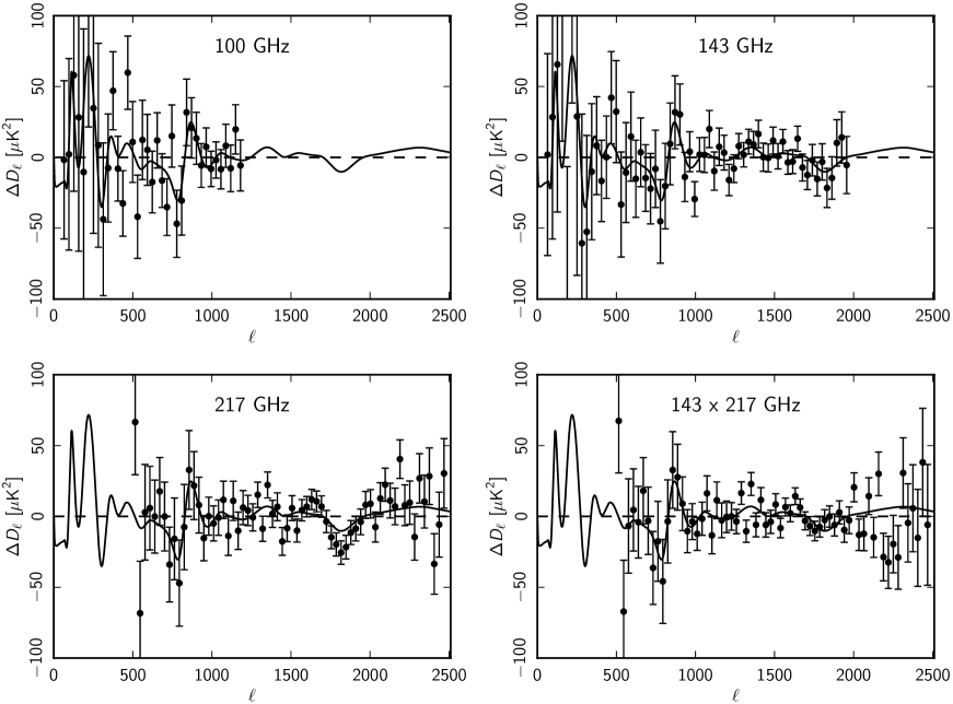
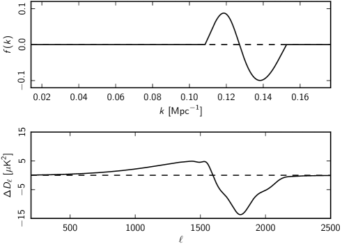
We found that simultaneously allowing extra degrees of freedom for small-scale structure and variations in the cosmological parameters changes the best fit fiducial model—that is, and —so that the variations with respect to the fiducial model no longer visibly gave the best straight line fit. Therefore we allow and to vary, so that the fiducial model is indeed the best straight line fit through the plotted data points. Detailed investigation showed that neither the priors, nor low- nor high- data play a significant role in determining the best fit fiducial model. This effect is small and within the error bars for and established assuming the fiducial model. To summarize, we maximize the likelihood with respect to the control points and the three cosmological parameters , , and . We then update the fiducial model ( and ) at each iteration by finding the best fit power law through the current best fit reconstruction.
Once the maximum likelihood solution has been found, the second derivatives about this solution are readily calculated by extracting the relevant matrices for most of the components, and estimating the remaining components using finite differences. The second derivative matrix is used to estimate the error on the reconstructed and the three cosmological parameters , , and . Monte Carlo simulations of a fiducial data set with a simplified CMB likelihood including some of the non-Gaussianities191919The simplified likelihood assumes full sky coverage and isotropic instrument noise. suggest that this approximation of the error is accurate for .
Figure 15 summarizes our results, showing the estimated in bins and the corresponding 1 and 2 errors. Errors in are also shown to represent the minimum reconstructible width evaluated at the middle of each bin. This is the minimum width that a Gaussian feature must have to be reconstructed with a small enough bias such that the mean reconstruction differs by less than 10% rms. The minimum reconstructible width is closely related to the correlation length, so that the errors between adjacent bins are weakly correlated and the total number of bins represents roughly the effective number of independent degrees of freedom.
While the plots with a significant roughness penalty—that is, with and —do not show any statistically significant evidence for features standing out above the noise of the reconstruction, for a smaller roughness penalty—that is, for and —a nominally statistically significant feature is clearly visible around We do not understand the origin of this feature, which may be primordial or may arise as a foreground or other systematic error in the high- portion of the likelihood. It should be noted that most of the robustness tests described in the likelihood paper assume smooth power spectra. The maximum excursions are locally at 3.2 and 3.9 for and respectively. In each of these two cases we correct for the look elsewhere effect by calculating the probability that one of the plotted error bars deviates by the same number of or more standard deviations. This calculation is carried out using the covariance matrix of the plotted error bars. We obtain and , which corresponds to 2.4 and 3.1, respectively. Additional simulations were carried out to validate the method by generating mock data according to the fiducial model and measuring the errors of the reconstruction obtained. These investigations confirm the error model. These tests were carried out both with and without test features. It can be argued that foregrounds are unlikely to explain the observed feature because all the foreground models involve smooth power law templates, whereas this feature is localized in multipole number. It is important to assess by means of a more extensive set of simulations whether the statistical significance assigned to this result is accurate.
We investigate which CMB angular multipoles correspond to this apparent feature. Figure 16 shows the residual from the reconstructed power spectrum with the best fit power law power spectrum subtracted together with the data for each of the frequency map correlation combinations used in the CamSpec likelihood. We observe a smooth dip around which is significant compared to the error bars, in particular for the 217 GHz map. To determine whether this dip is in fact responsible for large deviation in the reconstruction, we take the best fit reconstruction and set everywhere except for —the region where the large deviation is located—and calculate the corresponding spectrum. Figure 17 plots the residuals of this test feature, which show a large dip at around , thus demonstrating that the dip in the residual of the data centred at is responsible for the large excursions in the primordial power spectrum reconstructions.
Note added: The broad dip around in the temperature power spectrum, seen in the 217 GHz channel, has been shown to result from residuals that were strongest in the first survey. In work done after submission of this paper, this feature was shown to be associated with imperfectly subtracted electromagnetic interference generated by the drive electronics of the 4 K cooler and picked up by the detector read-out electronics. In a recent study, more aggressive measures were applied to remove 4 K contaminated data. When this censured data was propagated all the way to the maps and the power spectrum, the amplitude of the feature was lowered to below the noise for the first survey. A more complete account and analysis will appear in the next round of Planck cosmology papers.
8 Parametric searches for primordial power spectrum features
In this section we continue to investigate deviations of the primordial power spectrum from a smooth, featureless function, in this case by testing a set of theoretically motivated models.
8.1 Models and priors
We consider three models describing features in the primordial power spectrum: adding a global oscillation, a localized oscillation, or a cutoff to the large-scale power spectrum.
8.1.1 Wiggles model
Due to the exponential growth of the scale factor during inflation, a periodically recurring event in proper time which affects the amplitude of curvature perturbations would produce features that are periodic in . This occurs, for instance, for non Bunch-Davies initial conditions (Easther et al., 2001; Danielsson, 2002; Martin & Brandenberger, 2003; Bozza et al., 2003), or, e.g., in the axion monodromy model (Silverstein & Westphal, 2008), as a consequence of instanton induced corrections to the potential (Flauger et al., 2010). In these scenarios the primordial spectrum has an oscillation superimposed on an underlying smooth spectrum.
Here we consider the following parameterization of the primordial spectrum (referred to as the wiggles model):
| (50) |
with amplitude , frequency , and phase to quantify the superimposed oscillations. The underlying smooth spectrum has the standard power law form
| (51) |
The prior ranges for the wiggles model parameters are given in Table 10. The obvious prior for the phase is uniform over the interval We also choose a uniform prior on (a logarithmic prior on introduces considerable dependence of the resulting marginalized posteriors on the lower limit and does not contain the smooth spectrum as a limiting case). The sensitivity to primordial wiggles is limited at high frequencies by the width of the transfer function (Hamann et al., 2008a) and at low frequencies by the requirement of at least one full oscillation in the observable part of the power spectrum. Since Planck data are sensitive to wavenumbers over a range of roughly four orders of magnitude, this condition implies . Here we restrict the analysis to and assume a uniform prior. Larger values of the frequency are theoretically possible, e.g., in axion monodromy models (Flauger et al., 2010), but the amplitude of the oscillations in the s will be suppressed with respect to the primordial one. A comprehensive search for higher frequency oscillations is currently underway.
8.1.2 Step inflation model
If the slow roll of inflation is briefly interrupted, for instance by a phase transition (Starobinsky, 1992; Hunt & Sarkar, 2004), a burst of resonant particle production (Chung et al., 2000), or a step in the inflaton potential (Adams et al., 2001), or if the speed of sound changes suddenly (Achúcarro et al., 2011), a localized oscillatory feature is superimposed on the scalar primordial power spectrum. We adopt the approximate parameterization for such a feature from a step in the potential, introduced by Adshead et al. (2012), with
| (52) |
where
| (53) |
As in the wiggles model, we choose a uniform prior on the amplitude parameter (see Table 10). The parameter determines both the frequency of the feature and its location, which is required to lie in the observable range. The damping envelope of the feature is set by the ratio . We impose uniform priors on the logarithms of and .
8.1.3 Cutoff model
A number of models have been suggested to explain the apparent lack of power in the quadrupole and octupole of the WMAP temperature power spectrum. Typically in these models, the onset of a slow-roll phase coincides with the time when the largest observable scales exited the Hubble radius during inflation. This naturally suppresses the primordial power spectrum at large scales (see, e.g., Sinha & Souradeep, 2006). We consider a phenomenological parameterization of a cutoff proposed in Contaldi et al. (2003), given by
| (54) |
We apply uniform priors on , which determines the steepness of the cutoff, and on the logarithm of the cutoff scale .
| Model | Parameter | Prior range |
|---|---|---|
| Wiggles | [0, 0.2] | |
| [0.5, 100] | ||
| [0,] | ||
| Step inflation | [0, 0.2] | |
| [0, 12] | ||
| [-1, 5] | ||
| Cutoff | [-12, -4] | |
| [0, 15] |
8.2 Method
To achieve the necessary numerical precision for models with features in the primordial spectra, we modify the standard settings of the CAMB numerical code in order to calculate at each rather than interpolating and refine the grid in wavenumber for the numerical integration. These changes significantly slow down the computation. In the models considered here, the likelihood function has characteristics that make sampling difficult, such as extended plateaus and multiple isolated maxima, which render the Metropolis-Hastings algorithm inefficient. We therefore use the nested sampling algorithm implemented in the MultiNest add-on (Feroz & Hobson, 2008; Feroz et al., 2009) to CosmoMC (Lewis & Bridle, 2002), which can also calculate the Bayesian evidence and the likelihood profiles.
The signatures of the feature models considered here are unique and cannot be mimicked by varying other parameters, which lead to smooth variations of the power spectrum (with the exception of highly tuned very low frequency oscillations that can change the acoustic peak structure). We thus restrict ourselves to varying only the parameters describing the features and keep all remaining cosmological and nuisance parameters fixed to their CDM best fit values.202020An a posteriori maximization of the likelihood in a narrow parameter range around the best fit feature model parameters, including a variation of all remaining cosmological and nuisance parameters, shows that the change in the best fit is merely and hence does not affect our conclusions.
8.3 Results
For all three models we find that including these additional features improves the quality of the fit with respect to a pure power law spectrum. For the Planck+WP data, we show the best fit primordial curvature power spectra and temperature angular power spectrum residuals in Fig. 18, and report the best fit parameter values in Table 11. Since in all three cases the likelihood functions do not tend to zero in all directions of the respective parameter spaces, the Bayesian quantities (i.e., posterior distributions and Bayes factors) depend strongly on the choice of prior. For this reason, we also quote two prior-independent quantities, the effective (i.e., and the profile as a function of selected model parameters plotted alongside the marginalized posteriors in Fig. 19, which illustrates the unconventional shape of the likelihood functions.

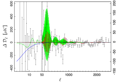
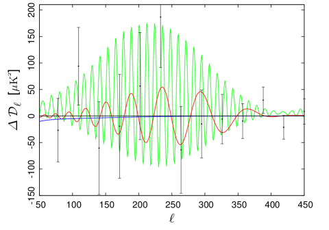
For the wiggles model, oscillations around the first acoustic peak and in the range improve the fit to the data, whereas for the best fit step inflation model the spectrum between the Sachs-Wolfe plateau and the first acoustic peak is fit better. Quantitatively, the cutoff model improves the fit only modestly, with , but both the wiggles and step inflation models lead to a larger improvement, with , at the cost of three new parameters. Already for pre-Planck data, improvements of have been reported in related analyses (e.g., Peiris et al. 2003; Martin & Ringeval 2004; Elgarøy et al. 2003; Covi et al. 2006; Meerburg et al. 2012; Benetti et al. 2013; Peiris et al. 2013). Note that in the step inflation model, the best fit does not coincide with the maximum of the marginalized posterior probability, indicating that some degree of fine tuning is necessary to reach the maximum of the likelihood. The maximum of the marginalized posterior at actually reproduces the feature at found previously in WMAP data (Peiris et al., 2003). The secondary peak at corresponds to a feature at multipoles where the analysis of Sect. 7 found a feature. However the model does not account for this feature well, yielding an improvement of only .
Whether or not these findings can be considered statistically significant or arise simply from overfitting noisy data is not a trivial question (see, for instance, the discussion in Bennett et al. (2011)). From a frequentist statistics point of view, an answer would require the rather involved procedure of repeating the analysis on a large set of simulations. In designing the test statistic, special care would need to be taken in making sure to take into account the look elsewhere effect (i.e., the fact that a particular observed anomaly may be very unlikely, whereas the probability of observing some anomaly may be much larger). From a Bayesian statistics point of view, it is the Bayesian evidence that can tell us how probable the extended models are, compared to the baseline power law primordial power spectrum.
For the models and the choice of prior probabilities considered here, the Bayesian evidence in fact favours, albeit weakly, the simple power law spectrum over the more complex models. The reason is that the Bayesian evidence punishes a lack of predictivity in these models. Most of the parameter space volume is not compatible with the data. A good match to observations is obtained within only a small subregion. Nonetheless, the observed features remain interesting since if they are real, they will also leave traces in other observabless, most notably, in the -mode polarization spectrum, where the signatures of features in the primordial spectrum are actually less washed out than in the temperature spectrum (Mortonson et al., 2009). The forthcoming Planck polarization data will prove very useful in this regard. Additionally, since strong deviations from power law behaviour typically indicate nonlinear physics, these models generically also predict a non-Gaussian signal potentially observable in the bispectrum (Planck Collaboration XXIV, 2014). However, the best fit wiggles and step inflation models have oscillations with a frequency too high to be accessible to bispectrum analysis at present.
| Model | Parameter | Best fit value | ||
|---|---|---|---|---|
| Wiggles | 1.5 | |||
| Step inflation | 0.3 | |||
| Cutoff | 0.3 | |||
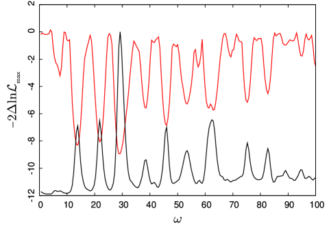

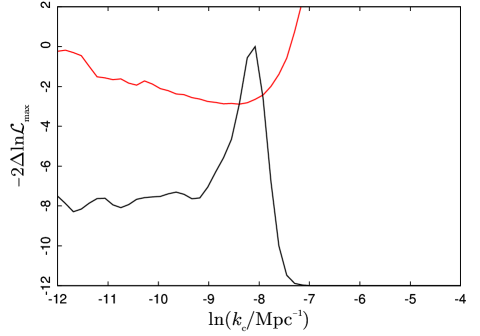
9 Combined analysis with Planck constraints for single field inflation
In the previous sections we have analysed inflationary models with a canonical kinetic term. This led to the tensor-to-scalar consistency condition requiring . It is interesting to consider more general classes of inflationary models characterized by a non-standard kinetic term (Garriga & Mukhanov, 1999) or more general higher-derivative operators (Kobayashi et al., 2010). An interesting subclass of these models are those in which the Lagrangian is a general function of the scalar inflaton field and its first derivative: , where . A more general extension is provided by the so-called effective field theory of inflation (Cheung et al., 2008), which has a richer phenomenology.
We restrict our analysis to the first class of models (Garriga & Mukhanov, 1999; Chen et al., 2007), which includes -inflation models (Armendáriz-Picón et al., 1999; Garriga & Mukhanov, 1999), and Dirac-Born-Infield (DBI) models introduced in the context of brane inflation (Silverstein & Tong, 2004; Alishahiha et al., 2004). In this class of models inflation can take place with a steep potential or can be driven by the kinetic term. One of the main features of inflationary models with a non-standard kinetic term is that the inflaton fluctuations can propagate at a sound speed . As shown in previous analyses (e.g., Peiris et al., 2007; Powell et al., 2009; Lorenz et al., 2008; Agarwal & Bean, 2009) there are strong degeneracies between the parameters determining the observable power spectra. Constraints on primordial non-Gaussianity can help break this degeneracy, and we show how Planck’s combined measurement of the power spectrum and the nonlinearity parameter (Planck Collaboration XXIV, 2014) improves constraints on this class of models.
In models with a non-standard kinetic term the sound speed of the inflaton is given by (Garriga & Mukhanov, 1999), so that in the canonical models, where , one finds , while in general a non-trivial corresponds to deviations from this standard case. Therefore, in these models, new parameters, such as the sound speed and its running, appear in the expressions for the inflationary observables. For the running of the sound speed it is useful to define an additional slow-roll parameter
| (55) |
For values of the slow-roll parameters much less than unity, the leading order scalar power spectrum is modified (Garriga & Mukhanov, 1999) to
| (56) |
which is evaluated at . The scalar spectral index gets an additional contribution from the running of the sound speed,
| (57) |
The gravitational sector remains unaltered by the non-trivial inflaton sound speed, retaining the same form as for the standard slow-roll models. Therefore the usual consistency relation is modified to with as usual (Garriga & Mukhanov, 1999). The more accurate relation employed in this analysis is
| (58) |
This accounts for the difference in freeze-out between the scalar and tensor perturbations (Peiris et al., 2007; Powell et al., 2009; Lorenz et al., 2008; Agarwal & Bean, 2009) taking place at for the scalar fluctuations, and at for the tensor modes.
Limiting ourselves to the predictions at lowest order in the slow-roll parameters, there are clearly degeneracies between the parameters (), which make the constraints on the inflationary power spectra observables less stringent in terms of these microscopic parameters. However, for models where the inflaton field has a non-standard kinetic term with , a high level of primordial non-Gaussianity of the scalar perturbations is generated (see, e.g., Chen et al., 2007). In these models primordial non-Gaussianity is produced by the higher-derivative interaction terms that arise when expanding the kinetic part of the Lagrangian, . The amplitude of the non-Gaussianity, defined by the nonlinearity parameter , receives two dominant contributions, arising from the inflaton interaction terms and . Each of them produces non-Gaussianity shapes similar to the so-called equilateral type (Babich et al. 2004), i.e., a signal that peaks for equilateral triangles . However, they are sufficiently distinct that the total signal can be very different from the equilateral one (Senatore et al., 2010). The nonlinearity parameter of the second interaction term is , while the other is determined by a second independent amplitude (Chen et al., 2007; Senatore et al., 2010). Constraints on the primordial non-Gaussianity, presented in the companion paper Planck Collaboration XXIV (2014), thus allow us to construct a lower limit for the sound speed . This helps reduce degeneracies in the parameter space of inflationary models with non-standard kinetic terms. In particular, without the limits on the sound speed coming from the constraints on primordial non-Gaussianity, it is not possible to derive an upper limit on the parameter , because the relation between the tensor-to-scalar ratio and also involves the sound speed (see, e.g., Eq. 58).
In this paper, we consider three cases. One is a general analysis as described above, where we focus on the simplest case of a constant speed of sound with . From the Planck limits on primordial non-Gaussianity in general single field models of inflation (Planck Collaboration XXIV, 2014), the most conservative constraint on the sound speed is
| (59) |
In this large parameter space, we assume a uniform prior in Eq. 58 within the HFF formalism described in the Appendix. We show the joint constraints on and in Fig. 20. By including the 95 CL constraint on from Eq. 59, Planck+WP constrain . Such constraints can be compared with the restricted case of , also shown in Fig. 20, with at 95% CL.

The other two cases analysed correspond to specific models where the inflaton has a non-standard kinetic term. The degeneracy between the different slow-roll parameters is broken because these models specifically predict that , or . As an example, we first consider the case where the action takes the Dirac-Born-Infield (DBI) form
| (60) |
Here is the potential and is the warp factor determined by the geometry of the extra dimensions. For DBI models a stronger bound on is derived (Planck Collaboration XXIV, 2014): at 95% CL. With the uniform prior and , Planck + WP constrain at 95% CL.
An important case is (for details, see Silverstein & Tong (2004), Alishahiha et al. (2004), Chen et al. (2007), and references therein). There are two possibilities. First, in ultraviolet (UV) DBI models, the inflaton field moves under a quadratic potential from the UV side of the warped space to the infrared side, with . It is known that this case is already at odds with observations if theoretical internal consistency of the model and constraints on power spectra and primordial non-Gaussianity are taken into account (Baumann & McAllister, 2007; Lidsey & Huston, 2007; Bean et al., 2007; Peiris et al., 2007; Bean et al., 2008). It is therefore interesting to look at the other case, namely infrared DBI models (Chen 2005b, a) where the inflaton field moves from the IR to the UV side, and the inflaton potential is
| (61) |
with a wide range of values allowed for in principle, (Bean et al., 2008). Here we focus on a minimal version of the IR DBI models where string effects are neglected, so that the usual field theory computation of the primordial curvature perturbation holds. For IR DBI models accounting for such effects and a more involved treatment of the dynamics, see Chen (2005a), Chen (2005c), and Bean et al. (2008). In this minimal IR DBI model, one finds (Chen, 2005c; Chen et al., 2007) , , and (in this model one can verify that ). Here primordial non-Gaussianity of the equilateral type is generated with an amplitude .
If we consider , then the predicted spectral index lies within the range , which is consistent with the Planck measurement of the spectral index at the 3 level, for . The constraints on non-Gaussianity give at CL (Planck Collaboration XXIV, 2014). Combining these constraints with the power spectrum constraints, marginalizing over , we obtain
| (62) |
This strongly limits the allowed parameter space of these models.
As a final example, we consider a class of power-law -inflation models characterized by the Lagrangian (Armendáriz-Picón et al., 1999)
| (63) |
In this case, for small values of one finds: , , . The sound speed is a constant (), with constant . The primordial non-Gaussianity in this model has an amplitude . Therefore, all the inflationary observables depend essentially on a single parameter . Imposing a prior of from the non-Gaussianity constraint at CL (Planck Collaboration XXIV, 2014), we obtain at CL. At the same time, our measurement of the spectral index constrains at CL. This class of -inflation models is therefore excluded by the combined constraints on primordial non-Gaussianity and the power spectrum.
10 Isocurvature modes
10.1 Theoretical background
In this section we explore the constraints imposed by Planck on scenarios where the primordial cosmological perturbations were not entirely adiabatic. These scenarios also include isocurvature modes, possibly correlated among themselves as well as with the adiabatic mode. The adiabatic mode is characterized by the property that at very early times the universe obeyed a common, spatially uniform equation of state and all components initially shared a common velocity field. For the adiabatic mode the density perturbations in the various components (i.e., baryons, CDM, photons, and neutrinos) are locked together. Here baryons include their accompanying leptons, assumed tightly coupled to maintain charge neutrality.
Isocurvature modes arise from spatial variations in the equation of state or from relative velocities between the components. To analyse how the CMB perturbations were imprinted, it is most convenient to define isocurvature modes at a sufficiently late time, such that the relevant components, according to our present best understanding, consisted of baryons, photons, CDM, and neutrinos. Under this hypothesis, in addition to the adiabatic mode there are four possible non-decaying isocurvature modes: the baryon, CDM, and neutrino density isocurvature modes, and the neutrino velocity isocurvature mode (see, e.g., Bucher et al. (2000) for a discussion and further references).
The impact of isocurvature modes on the CMB was first studied in detail by Peebles & Yu (1970) and Efstathiou & Bond (1986, 1987), who contemplated the possibility that isocurvature perturbations rather than adiabatic perturbations were the sole source of cosmological perturbations. Linde (1985), Polarski & Starobinsky (1994), Linde & Mukhanov (1997), and García-Bellido & Wands (1996) pointed out various scenarios in which isocurvature perturbations could be generated within the context of inflation. Bucher et al. (2000) carried out a systematic study of isocurvature modes from a phenomenological perspective, pointing out the relevance of two additional modes: the neutrino density and velocity modes. Lyth & Wands (2002), Moroi & Takahashi (2001), and Bartolo & Liddle (2002) studied an interesting so-called curvaton scenario, in which adiabatic fluctuations from inflation contribute negligibly, but quantum fluctuations in a transverse direction modulate the density of decaying particles, leading to isocurvature perturbations correlated with the adiabatic mode.
Several authors have studied the constraints on isocurvature modes imposed by previous microwave background experiments, including Stompor et al. (1996), Langlois & Riazuelo (2000), Amendola et al. (2002), Peiris et al. (2003), Valiviita & Muhonen (2003), Bucher et al. (2004), Moodley et al. (2004), Beltran et al. (2004), Kurki-Suonio et al. (2005), Dunkley et al. (2005), Bean et al. (2006), Trotta (2007), Keskitalo et al. (2007), and Komatsu et al. (2009). A more complete set of references may be found in Valiviita et al. (2012).
Before proceeding we must define precisely how to characterize these isocurvature modes on super-Hubble scales during the epoch after entropy generation, during which we assume that the stress-energy content of the universe can be modelled as a multi-component fluid composed of baryons, CDM particles, photons, and neutrinos. If we assume that the evolution of the universe during this epoch was adiabatic (used here in the sense of thermodynamically reversible), then the entropy per unit comoving volume is conserved and serves as a useful reference with respect to which the abundances of the other components can be expressed.
The baryon isocurvature mode may be expressed in terms of fractional fluctuations in the baryon-to-entropy ratio, which is conserved on super-Hubble scales during this epoch. The CDM and neutrino density isocurvature (NDI) modes may be defined analogously. The neutrino velocity isocurvature (NVI) mode refers to fluctuations in the neutrino velocity relative to the average bulk velocity of the cosmic fluid. For the CMB, the baryon and CDM isocurvature modes yield almost identical angular spectra because the deficit of one is balanced by an excess of the other, so we do not consider them separately here. In this way the primordial isocurvature modes may be defined as dimensionless stochastic variables , , , like the variable describing the adiabatic mode.212121The symbol is sometimes used in the literature to denote the isocurvature modes, also known as entropy perturbations. To prevent confusion we avoid this terminology because isocurvature modes are unrelated to any notion of thermodynamic entropy. In this basis, the CDI mode can be seen as an effective isocurvature mode, encoding both CDM and baryon isocurvature fluctuations through (Gordon & Lewis, 2003).
Within this framework, Gaussian fluctuations for the most general cosmological perturbation are described by a positive definite matrix-valued power spectrum of the form
| (64) |
Following the conventions used in CAMB (Lewis & Bridle, 2002; Lewis, 2011) and CLASS (Lesgourgues, 2011; Blas et al., 2011), the primordial isocurvature modes are normalized as follows in the synchronous gauge: for the CDI mode, is the primordial power spectrum of the density contrast for the NDI mode it is that of and for the NVI mode, that of the neutrino velocity times 4/3. 222222In other words, of the neutrino perturbation dipole, in the notation of Ma & Bertschinger (1995).
If isocurvature modes are present, the most plausible mechanism for exciting them involves inflation with a multi-component inflaton field. To have an interesting spectrum on the large scales probed by the CMB, isocurvature modes require long-range correlations. Inflation with a multi-component inflaton provides a well motivated scenario for establishing such correlations. Inflation with a single-component scalar field can excite only the adiabatic mode. In models of inflation with light (compared to the Hubble expansion rate) transverse directions, the scalar field along these transverse directions becomes disordered in a way described by an approximately scale-invariant spectrum. If the inflaton has light components, there are potential isocurvature modes during inflation. Whether or not the fluctuations along these transverse directions are subsequently transformed into the late-time isocurvature modes described above depends on the details of what happens after inflation, as described more formally below.
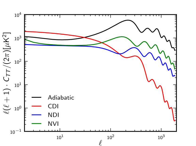
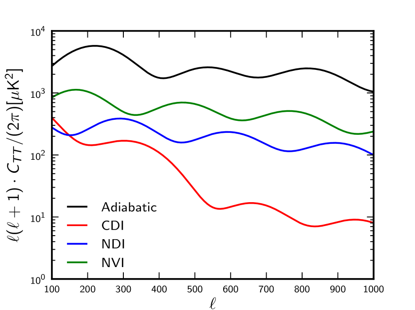
As explained for example in Langlois (1999), Gordon et al. (2001), Groot Nibbelink & van Tent (2000, 2002), and Byrnes & Wands (2006), for inflationary models where the inflaton follows a curved trajectory, correlations are generically established between the isocurvature and curvature degrees of freedom. To lowest order in the slow-roll approximation, this leads to a situation where the adiabatic perturbation is the sum of several components each of differing spectral index.
The post-inflationary evolution determines how the isocurvature fluctuations generated during inflation transmute into the three specific isocurvature modes studied here. Little is known about the details of what happens during the epoch of entropy generation, but to linear order we may express how the fields (i.e., the curvature perturbation at the end of inflation) and the transverse components of the inflaton field (i.e., the components orthogonal to the slow-roll direction) transform into curvature perturbations and late-time isocurvature modes at the end of the epoch of entropy generation as the linear transformation
| (65) |
where BI, CDI, NDI, NVI, while labels the transverse components of the component inflaton field. Physically, the fluctuations along the transverse directions modulate particle production during the epoch of entropy generation.
The neutrino density isocurvature can be excited in much the same way as the CDM and baryon isocurvature mode because at least within the standard electroweak model, in which there are no leptonic flavour changing processes, and are separately conserved. Known non-perturbative processes such as the sphaleron can trade lepton and baryon asymmetries with each other and alter flavour asymmetries, but they cannot erase such asymmetries altogether. Plausible models generating the neutrino density mode are therefore possible (Bucher et al., 2000; Gordon & Malik, 2004), but as for the neutrino velocity isocurvature mode, to date no plausible generation mechanism has been put forth.
This extension of the adiabatic CDM model to non-adiabatic initial conditions represents an important test of inflation. Single-field inflation can produce only adiabatic perturbations, since exciting isocurvature perturbations requires additional degrees of freedom during inflation. Therefore a detection of primordial isocurvature perturbations would point to more complicated models of inflation.
10.2 Adiabatic with one isocurvature mode and free spectral indices
In this paper we investigate three of the four possible isocurvature modes of the CDM scenario, since the baryon and CDM isocurvature perturbations are indistinguishable in the CMB angular power spectra. The CDM, neutrino density, and neutrino velocity isocurvature perturbations lead to different power spectra for CMB anisotropies, as shown in Fig. 21. We limit ourselves to studying one isocurvature mode at a time, in the presence of a curvature perturbation. More general combinations with two or three isocurvature modes may be contemplated, but without the Planck high frequency polarization likelihood, it is difficult to constrain such scenarios, so we postpone a discussion of this case to the next release.
Theoretically, one expects the power spectra of the isocurvature modes and their correlations to exhibit near but not necessarily exact scale invariance. As a general test of adiabaticity, it is nevertheless interesting to compare a more general model to the Planck data, assuming that the adiabatic, isocurvature, and cross-correlation spectra obey power laws with free spectral indices. Blue values of the spectral indices are particularly interesting from the point of view of testing adiabaticity, because the acoustic peaks arising from two of the isocurvature modes are out of phase with the adiabatic peaks by roughly near the first acoustic peak. This is not true for the neutrino velocity isocurvature mode however.
In the literature, models with one isocurvature as well as the adiabatic mode (possibly correlated) are often parameterized by specifying the correlation matrix at a certain pivot scale wth components along with their respective spectral indices (e.g., Amendola et al., 2002; Beltran et al., 2004). We do not follow this approach because in the absence of a statistically significant detection, the posterior distributions for the spectral indices are difficult to interpret and sensitive to how the prior is chosen. We instead adopt a parameterization where is specified at two scales and and interpolated geometrically according to232323 Although the models spanned by the one-scale and two-scale parameterizations are the same, the priors for these parameterizations are related by a non-constant Jacobian and therefore do not coincide.
| (66) | ||||
where and , or . We set and so that spans most of the range in constrained by Planck data. A uniform prior for the components is assumed, where auto-correlation amplitudes are positive, although the cross-correlation amplitudes may take both signs subject to the constraints
| (67) |
to ensure positive definiteness. For the logarithm of the off-diagonal elements in Eq. 66 to be real, we must have . This Ansatz can be trivially modified to admit the case by inserting appropriate minus signs, but this parameterization does not allow the case where the sign of the correlation changes. In practice we deal with this by assuming a uniform prior not on , but on its absolute value, and then we impose . The constraints in Eq. 67 ensure that is positive definite within the interval but generically positive definiteness is violated sufficiently far outside this interval, either for very small or very large Where this happens we reduce the magnitude of so that there is either total correlation or anti-correlation. The kinks thus introduced lie outside the range Within this range, the spectral indices are scale-independent. Finally, our sign conventions are such that positive values for correspond to a positive contribution of the cross-correlation term to the Sachs-Wolfe component of the total temperature spectrum.
When the constraining power of the data is weak, a crucial question is to what extent the posterior distribution results from the data rather than from the prior distribution. The parameterization above is not the only one that could have been adopted, and other possible priors are typically related by a non-constant Jacobian. For each model, we indicate the log-likelihood for the best fit model, in order to allow model comparison.
The Planck+WP results for the three isocurvature modes using this two-scale parameterization are shown in Fig. 22 and included in the summary Table 12. The power spectra and are normalized according to the primordial values of the fields and defined above. It is interesting to consider how much isocurvature power is allowed expressed as a fraction of the power in three bands spanning the CMB temperature spectrum observed by Planck. To this end, we define the following derived quantities
| (68) | ||||
| (69) | ||||
| (70) |
where
| (71) |
The 95% confidence limits from the one-dimensional posterior distributions for these fractional contributions in the full range are shown in Table 12. The range of allowed values for is a measure of the adiabaticity of fluctuations in the CMB. The posterior distributions of the fractions in three multipole ranges are shown in Fig. 23. We also report the primordial isocurvature fraction, defined as
| (72) |
at three values of . Table 12 also shows the effective for all models, compared to the minimal six-parameter CDM model. In Fig. 24 we show the ratio of temperature spectra for the best fit mixed model to the adiabatic model.


| Model | ||||||||
|---|---|---|---|---|---|---|---|---|
| General model: | ||||||||
| CDM isocurvature | 0.075 | 0.39 | 0.60 | [0.98:1.07] | 0.039 | [-0.093:0.014] | 4 | -4.6 |
| ND isocurvature | 0.27 | 0.27 | 0.32 | [0.99:1.09] | 0.093 | [-0.18:0] | 4 | -4.2 |
| NV isocurvature | 0.18 | 0.14 | 0.17 | [0.96:1.05] | 0.068 | [-0.090:0.026] | 4 | -2.5 |
| Special CDM isocurvature cases: | ||||||||
| Uncorrelated, (“axion”) | 0.036 | 0.039 | 0.040 | [0.98:1] | 0.016 | – | 1 | 0 |
| Fully correlated, (“curvaton”) | 0.0025 | 0.0025 | 0.0025 | [0.97:1] | 0.0011 | [0:0.028] | 1 | 0 |
| Fully anti-correlated, | 0.0087 | 0.0087 | 0.0087 | [1:1.06] | 0.0046 | [-0.067:0] | 1 | -1.3 |
The results for show that the nonadiabatic contribution to the temperature variance can be as large as 7% (9%, 5%) in the CDI (NDI, NVI) model (at 95% CL). These results are driven by the fact that on large scales, for , the Planck data points on average have a slightly smaller amplitude than the best fitting CDM model. Hence the data prefer a significant amount of anticorrelated isocurvature modes, leading to a reduction of amplitude of the Sachs-Wolfe plateau and to a decrease of the effective by up to 4.6.242424For the three general models, the posterior distribution is actually multimodal. Here we are referring to models contributing to the main peak in the posterior, with the highest maximum likelihood. There is another peak with a smaller maximum likelihood, appearing in Fig. 23 as a small bump for positive values of the cross-correlation amplitude. In this paper, we do not carry out a separate investigation for models contributing to this secondary peak. This situation explains the rather loose bounds on the derived parameter , as shown in Fig. 23.
A comparison of and shows that best fitting models have an isocurvature spectral index close to 1.7 for CDI, 1.1 for NDI, and 1.0 for NVI modes.
For CDI and NDI, the amplitude of acoustic peaks quickly decreases with increasing , so that the constraints are entirely driven by small s. Since the same value of the primordial amplitude leads to different plateau amplitudes for the two isocurvature models (see Fig. 21), the bounds on and are consistently stronger for CDI than for NDI. For NVI, the acoustic peak amplitude is larger than the plateau amplitude. In NVI models, the data cannot allow for a too large amplitude of correlated isocurvature modes at small , because the total spectrum would be distorted at larger . This possibility is strongly disfavoured by the data, which are consistent with the peak location predicted by a pure adiabatic model. Hence in the NVI case we obtain slightly stronger bounds and a smaller reduction of the effective .
The fact that the data prefer models with a significant contribution from CDI or NDI modes should be interpreted with care. The detection of a shift in the phase of acoustic oscillations would bring unambigous evidence in favour of isocurvature modes. With Planck data, we are not in this situation. The evidence is driven by a small deficit of amplitude in the Sachs-Wolfe plateau, which could have several different possible explanations (such as a deficit in the large-scale primordial power spectrum, as already seen in the previous sections). However, multi-field inflationary scenarios can produce the mixture of curvature and isocurvature fluctuations which we have found to provide a good fit to the Planck data.
10.3 Special cases
The six-parameter models of the previous subsection including one isocurvature mode and the adiabatic mode make no assumptions about the spectral indices of each mode or the degree of correlation between the isocurvature mode and the adiabatic mode. This leads to a large number of additional degrees of freedom. There are both theoretical and phenomenological motivations for choosing special values for some of the parameters, leading to special cases with just one more degree of freedom with respect to the adiabatic case. The results are reported in Table 12, for uncorrelated perturbations with , and fully correlated or anti-correlated perturbations with . In the general case, anti-correlated isocurvature perturbations slightly improve the fit to the Planck data. We consider below the implications of our results for two important cases: the axion and curvaton scenarios.
10.3.1 Constraints on axion isocurvature
The axion field was proposed to solve the strong CP problem and constitutes a well-motivated dark matter candidate. (See for example Preskill et al. (1983), Turner (1990), Peccei (2008), Sikivie (2008), Raffelt (2008), and Kim & Carosi (2010)). The axion is the psuedo-Goldstone boson of the broken Peccei-Quinn (PQ) symmetry. Under certain assumptions, the axion field may induce significant isocurvature perturbations (Turner et al., 1983; Axenides et al., 1983; Steinhardt & Turner, 1983; Linde, 1984, 1985; Seckel & Turner, 1985; Kofman, 1986; Lyth, 1990; Linde & Lyth, 1990; Turner & Wilczek, 1991; Linde, 1991; Lyth, 1992). If inflation takes place after PQ symmetry breaking, the quantum fluctuations of the inflaton are responsible for primordial curvature perturbations, while those of the axion field generate primordial entropy perturbations. After the QCD transition, when one of the vacua becomes preferred giving the axion field a mass, the axions behave as cold dark matter. This way of producing axionic dark matter is called the misalignment angle mechanism. In such a scenario, the CMB anisotropy may include significant power from CDM isocurvature fluctuations. In that case, the fraction of CDM isocurvature modes is related to the energy scale of inflation, , through (Lyth, 1990; Beltran et al., 2007; Bae et al., 2008; Hamann et al., 2009)
| (73) |
where is the relic axion density, the fraction of CDM consisting of axions, and the PQ symmetry breaking scale. In this model, CDM isocurvature perturbations should be totally uncorrelated with adiabatic perturbations and have a spectral index very close to one since in the first-order slow-roll approximation the index reads . Since the sensitivity of the data to is very limited (Beltran et al., 2007), we assume for simplicity that .
Within the general parametrization presented in Eq. 66, we can select the axion case by imposing , as well as the condition
| (74) |
corresponding to . We therefore have three independent parameters, and , and we sample these parameters with uniform prior distributions. The fraction with Mpc-1 is then a derived parameter. Since the data constrain , the relation between and is nearly linear, so the primordial isocurvature fraction is sampled with a close to uniform prior.
Constraints on this model are shown in Table 12. We find
| (75) |
at the scale , with a best fit value of zero. Hence there is no evidence for axion generated isocurvature perturbations. This limit significantly improves the previous CMB bounds. At the scale Mpc-1, our result reads , to be compared to for WMAP 9-year alone, or for WMAP+ACT+SPT at 95% CL (Hinshaw et al., 2013). This bound can be used to exclude regions of parameter space composed of , , and the energy scale of inflation, but cannot be used to obtain a model-independent bound on . However, if we assume (i) that the PQ symmetry is broken during inflation, (ii) that it is not restored by the quantum fluctuations of the inflaton (which imposes ), nor by thermal fluctuations in case of a very efficient reheating stage, and (iii) that all the CDM consists of axions produced by the misalignment angle, then we can derive an upper bound on the energy scale of inflation as
| (76) |
10.3.2 Constraints on the curvaton scenario
In the simplest one-field inflationary models curvature perturbations arise from quantum fluctuations in the inflaton field, but this is not the only way to generate curvature perturbations. Isocurvature perturbations may seed curvature perturbations outside the Hubble radius (Polarski & Starobinsky, 1994; Langlois, 1999; Gordon et al., 2001), so it is possible that a significant component of the observed adiabatic mode could be strongly correlated with an isocurvature mode. This happens for instance in the curvaton scenario (Mollerach, 1990; Enqvist & Sloth, 2002; Moroi & Takahashi, 2001; Lyth & Wands, 2002; Lyth et al., 2003; Gordon & Lewis, 2003). The curvaton is an extra light scalar field acquiring a spectrum of fluctuations on cosmological scales during inflation. Depending on its density evolution and decay history, this field could be responsible for part of the observed adiabatic perturbations, or all of them, or for a mixture of correlated adiabatic and isocurvature perturbations.
We focus here on the simplest viable version of this scenario in which the curvaton decays into CDM particles while contributing a non-negligible fraction
| (77) |
to the total energy density of the universe. If the curvaton dominates at decay time (), its primordial fluctuations seed curvature perturbations equivalent to a pure adiabatic mode. If , curvaton fluctuations are only partially converted into adiabatic perturbations, while CDM particles carry CDI perturbations, which are fully correlated with the adiabatic perturbations since they share a common origin. We recall that with our conventions, “fully correlated” means that the cross-correlation term contributes constructively to the Sachs-Wolfe component of the total temperature spectrum. Some authors define the correlation with the opposite sign and call this case “fully anti-correlated” (e.g., Komatsu et al., 2011; Hinshaw et al., 2013). In this model, the CDI fraction is related to by (Gordon & Lewis, 2003)
| (78) |
In our notation this is equivalent to
| (79) |
Within the general parametrization presented in Eq. 66, we can satisfy this case by imposing
| (80) |
together with the condition
| (81) |
corresponding to . As in the axion case, this results in three independent parameters and which we sample with uniform priors. The constraints for this model are shown in Table 12. The best fit model is still the pure adiabatic case, and the upper bound
| (82) |
is scale independent, since the adiabatic and isocurvature tilts are assumed to be equal. This is a significant improvement over the WMAP 9-year bounds, for WMAP alone, or for WMAP+ACT+SPT at 95% CL (Hinshaw et al., 2013). We conclude that in this scenario, the curvaton should decay when it dominates the energy density of the universe, with .
The nonlinearity parameter in the curvaton model studied here is (Bartolo et al., 2004c, b)
| (83) |
assuming a quadratic potential for the curvaton field (Sasaki et al., 2006). In the pure adiabatic case () this leads to . The constraint then corresponds to . Taking into account the Planck result (Planck Collaboration XXIV, 2014), we conclude that the Planck data are consistent with the scenario where the curvaton decays into CDM when it dominates the energy density of the universe, and its fluctuations are almost entirely converted into adiabatic ones.
11 Conclusions
This paper establishes the status of cosmic inflation in the context of the first release of the Planck cosmological results, which includes the temperature data from the first sky surveys. CMB polarization as measured by Planck will be the subject of a future release. We find that standard slow-roll single-field inflation is compatible with the Planck data. This result is confirmed by other papers of this series. Planck in combination with WMAP 9-year large angular scale polarization (WP) yields at 95% CL by combining temperature and lensing information (Planck Collaboration XVI, 2014; Planck Collaboration XVII, 2014). The bispectral non-Gaussianity parameter measured by Planck is consistent with zero (Planck Collaboration XXIV, 2014). These results are compatible with zero spatial curvature and a small value of as predicted in the simplest slow-roll inflationary models.
A key Planck result is the measurement of the scalar perturbation spectral index. Planck+WP data give (and when combined with BAO). This result disfavours the Harrison-Zeldovich (HZ) model at more than 5. Even in extended cosmological models, the HZ spectrum cannot be reconciled with the data. Allowing a general reionization scenario yields with respect to CDM for Planck+WP data. When the primordial helium abundance or the effective number of neutrino species are allowed to vary, the best fit of the HZ model to a combination of Planck+WP and BAO data is still worse by and , respectively.
We find no evidence for Planck data preferring a generalization of a simple power law spectrum to include a running of the spectral index () or a running of the running ( with Planck+WP). In a model admitting tensor fluctuations, the CL bound on the tensor-to-scalar ratio is () using Planck+WP (plus high- CMB data). This bound on implies an upper limit for the inflation energy scale of GeV, or equivalently, for the Hubble parameter , at CL.
The degeneracy between and which plagued previous CMB measurements, is now removed by the Planck precision in the determination of the highest acoustic peaks. Inflaton potentials with a concave shape are favoured and occupy most of the 95% confidence region allowed by Planck+WP in the plane. Models with an exponential potential, a monomial potential with a power larger than two, or hybrid models driven by a quadratic term are disfavoured at more than 95% confidence. The quadratic large-field model, in the past often cited as the simplest inflationary model, now lies at the edge of the 95% CL contours allowed by Planck+WP+high- CMB data.
A Bayesian parameter estimation and model comparison analysis of a representative sample of single-field slow-roll models shows that Planck is able to discriminate between these models with results that are robust even when a broad set of entropy generation scenarios are allowed. In addition to confirming the exclusion of the potential, the Bayesian evidence computed from the Planck data provides significant odds (logarithms of the Bayes factor of about or lower relative to CDM) against large-field models compatible with previous cosmological data, such as the potential, and two-parameter potentials such as natural inflation and the hilltop potential. As presented in Sect. 5, Planck establishes strong constraints on the parameter values of specific inflationary scenarios. For example, the scale parameter of the natural inflation potential is constrained to be (95% CL), improving upon the WMAP 7-year limit on by a factor of two. The Planck data limit the possibilities for the unexplored physics between the end of inflation and the beginning of the radiation dominated era. Data-driven constraints are obtained on , the effective equation of state in the post-inflationary era. Particularly for the disfavoured models listed above, their parameters are pushed to unnatural values () in order to become more compatible with the data.
Using an essentially exact numerical calculation of the predicted primordial spectrum, we reconstruct the observable window of the inflaton potential, expanding the potential as a Taylor series up to a fixed order. For an observable potential described by a polynomial of order three, the reconstruction agrees well with the slow-roll predictions. If a quartic term is allowed, the result deviates from the slow-roll prediction because the Planck data favour a slightly smaller amplitude for the Sachs-Wolfe plateau relative to the part of the power spectrum than the best fitting minimal CDM model with a power law primordial spectrum. A potential with a fourth-order polynomial can fit this feature, thus reducing the effective by approximately four.
A penalized likelihood reconstruction of the primordial power spectrum shows hints of structure at modest statistical significance. However, recent work after submission suggests that this feature can be explained by electromagnetic interference. Parameterized models producing superimposed oscillations (possibly motivated by deviations from the Bunch-Davies vacuum state, axion monodromy, or a sharp step in the inflaton potential) improve the by roughly , where three extra parameters have been added. However, a Bayesian model comparison analysis does not strongly favour the model with oscillations over the standard featureless power spectrum. With Planck polarization data, a more conclusive result on superimposed oscillations is expected.
We combine power spectrum constraints with those on the nonlinearity parameter (Planck Collaboration XXIV, 2014) to constrain single-field inflation with generalized Lagrangians, in which non-Gaussianities are larger than those predicted by the simplest slow-roll inflationary models. We show how the limits on the inflation sound speed derived in Planck Collaboration XXIV (2014) are crucial to constrain slow-roll parameters for generalized Lagrangians. We also show how particular examples of DBI Inflation and -inflation can be constrained by this combination of Planck data.
We test the hypothesis that the primordial cosmological perturbations were exclusively adiabatic. We analyse all nonsingular (i.e., nondecaying) isocurvature modes arbitrarily correlated to the adiabatic mode, using a parameterization where the isocurvature contributions are specified at two scales. The oscillatory pattern in the Planck temperature spectrum is compatible with purely adiabatic perturbations, and therefore constrains any isocurvature contribution to be small at those multipoles. As a consequence, axion and curvaton scenarios, in which the CDM isocurvature mode is uncorrelated or fully correlated with the adiabatic mode, are not favoured by Planck. The upper bounds on the isocurvature fraction at Mpc-1 are for the axion, and for the curvaton, at 95% CL. However general models with an arbitrarily correlated mixture of adiabatic and (CDM or neutrino) isocurvature modes have the freedom to lower the Sachs-Wolfe plateau relative to the high- spectrum, and reduce the effective by more than four.
The simplest inflationary models have passed an exacting test with the Planck data. The full mission data including Planck’s polarization measurements will help answer further fundamental questions, helping to probe nonsmooth power spectra and the energy scale of inflation as well as extensions to more complex models.
Acknowledgements.
The development of Planck has been supported by: ESA; CNES and CNRS/INSU-IN2P3-INP (France); ASI, CNR, and INAF (Italy); NASA and DoE (USA); STFC and UKSA (UK); CSIC, MICINN, JA and RES (Spain); Tekes, AoF and CSC (Finland); DLR and MPG (Germany); CSA (Canada); DTU Space (Denmark); SER/SSO (Switzerland); RCN (Norway); SFI (Ireland); FCT/MCTES (Portugal); and PRACE (EU). A description of the Planck Collaboration and a list of its members, including the technical or scientific activities in which they have been involved, can be found at http://www.sciops.esa.int/index.php?project=planck&page=Planck_Collaboration. We gratefully acknowledge CINECA (http://www.cineca.it/) under the agreement LFI/CINECA and IN2P3 Computer Center (http://cc.in2p3.fr) for providing a significant amount of the computing resources and services needed for this work.References
- Abbott & Wise (1984) Abbott, L. & Wise, M. B. 1984, Nucl. Phys., B244, 541
- Achúcarro et al. (2011) Achúcarro, A., Gong, J.-O., Hardeman, S., Palma, G. A., & Patil, S. P. 2011, JCAP, 1101, 030
- Acquaviva et al. (2003) Acquaviva, V., Bartolo, N., Matarrese, S., & Riotto, A. 2003, Nucl. Phys. B, 667, 119
- Adams et al. (1993) Adams, F. C., Bond, J. R., Freese, K., Frieman, J. A., & Olinto, A. V. 1993, Phys. Rev., D47, 426
- Adams et al. (2001) Adams, J., Cresswell, B., & Easther, R. 2001, Phys. Rev. D, 64, 123514
- Adams et al. (2001) Adams, J. A., Cresswell, B., & Easther, R. 2001, Phys. Rev., D64, 123514
- Adshead et al. (2012) Adshead, P., Dvorkin, C., Hu, W., & Lim, E. A. 2012, Phys. Rev., D85, 023531
- Adshead et al. (2011) Adshead, P., Easther, R., Pritchard, J., & Loeb, A. 2011, JCAP, 1102, 021
- Agarwal & Bean (2009) Agarwal, N. & Bean, R. 2009, Phys. Rev. D, 79, 023503
- Akaike (1974) Akaike, H. 1974, IEEE Trans. on Automatic Control, 19, 716
- Albrecht & Steinhardt (1982) Albrecht, A. & Steinhardt, P. J. 1982, Phys. Rev. Lett., 48, 1220
- Alishahiha et al. (2004) Alishahiha, M., Silverstein, E., & Tong, D. 2004, Phys. Rev. D, 70, 123505
- Allahverdi et al. (2010) Allahverdi, R., Brandenberger, R., Cyr-Racine, F.-Y., & Mazumdar, A. 2010, Ann. Rev. Nucl. Part. Sci., 60, 27
- Amendola et al. (2002) Amendola, L., Gordon, C., Wands, D., & Sasaki, M. 2002, Phys.Rev.Lett., 88, 211302
- Anantua et al. (2009) Anantua, R., Easther, R., & Giblin, J. T. 2009, Phys. Rev. Lett., 103, 111303
- Anderson et al. (2012) Anderson, L., Aubourg, E., Bailey, S., et al. 2012, MNRAS, 427, 3435
- Armendáriz-Picón et al. (1999) Armendáriz-Picón, C., Damour, T., & Mukhanov, V. 1999, Phys. Lett. B, 458, 209
- Audren et al. (2012) Audren, B., Lesgourgues, J., Benabed, K., & Prunet, S. 2012, JCAP, 1302, 001
- Aver et al. (2012) Aver, E., Olive, K. A., & Skillman, E. D. 2012, JCAP, 1204, 004
- Axenides et al. (1983) Axenides, M., Brandenberger, R. H., & Turner, M. S. 1983, Phys. Lett., B126, 178
- Babich et al. (2004) Babich, D., Creminelli, P., & Zaldarriaga, M. 2004, JCAP, 8, 9
- Bae et al. (2008) Bae, K. J., Huh, J.-H., & Kim, J. E. 2008, JCAP, 0809, 005
- Banks et al. (1994) Banks, T., Kaplan, D. B., & Nelson, A. E. 1994, Phys. Rev., D49, 779
- Bardeen et al. (1983) Bardeen, J. M., Steinhardt, P. J., & Turner, M. S. 1983, Phys. Rev., D28, 679
- Barrow (1990) Barrow, J. D. 1990, Phys. Lett., B235, 40
- Barrow & Liddle (1993) Barrow, J. D. & Liddle, A. R. 1993, Phys. Rev., D47, 5219
- Bartolo et al. (2004a) Bartolo, N., Komatsu, E., Matarrese, S., & Riotto, A. 2004a, Phys. Rept., 402, 103
- Bartolo & Liddle (2002) Bartolo, N. & Liddle, A. R. 2002, Phys.Rev., D65, 121301
- Bartolo et al. (2004b) Bartolo, N., Matarrese, S., & Riotto, A. 2004b, Phys. Rev. Lett., 93, 231301
- Bartolo et al. (2004c) Bartolo, N., Matarrese, S., & Riotto, A. 2004c, Phys. Rev., D69, 043503
- Barvinsky et al. (2008) Barvinsky, A. O., Kamenshchik, A. Y., & Starobinsky, A. A. 2008, JCAP, 0811, 021
- Baumann & McAllister (2007) Baumann, D. & McAllister, L. 2007, Phys. Rev. D, 75, 123508
- Bean et al. (2008) Bean, R., Chen, X., Peiris, H., & Xu, J. 2008, Phys. Rev. D, 77, 023527
- Bean et al. (2006) Bean, R., Dunkley, J., & Pierpaoli, E. 2006, Phys. Rev., D74, 063503
- Bean et al. (2007) Bean, R., Shandera, S. E., Tye, S.-H. H., & Xu, J. 2007, JCAP, 5, 4
- Beltran et al. (2007) Beltran, M., García-Bellido, J., & Lesgourgues, J. 2007, Phys. Rev., D75, 103507
- Beltran et al. (2004) Beltran, M., García-Bellido, J., Lesgourgues, J., & Riazuelo, A. 2004, Phys. Rev., D70, 103530
- Benetti et al. (2013) Benetti, M., Pandolfi, S., Lattanzi, M., Martinelli, M., & Melchiorri, A. 2013, Phys. Rev., D87, 023519
- Bennett et al. (2011) Bennett, C., Hill, R., Hinshaw, G., et al. 2011, ApJS, 192, 17
- Bennett et al. (2013) Bennett, C., Larson, D., Weiland, J., et al. 2013, ApJS, 208, 20
- Beutler et al. (2011) Beutler, F., Blake, C., Colless, M., et al. 2011, MNRAS, 416, 3017
- Bezrukov & Gorbunov (2012) Bezrukov, F. & Gorbunov, D. 2012, Phys. Lett., B713, 365
- Bezrukov & Shaposhnikov (2008) Bezrukov, F. & Shaposhnikov, M. 2008, Phys. Lett., B659, 703
- Bezrukov & Shaposhnikov (2009) Bezrukov, F. & Shaposhnikov, M. 2009, JHEP, 07, 089
- Binétruy & Gaillard (1986) Binétruy, P. & Gaillard, M. K. 1986, Phys. Rev., D34, 3069
- Blas et al. (2011) Blas, D., Lesgourgues, J., & Tram, T. 2011, JCAP, 1107, 034
- Boubekeur & Lyth (2005) Boubekeur, L. & Lyth, D. 2005, JCAP, 0507, 010
- Bozza et al. (2003) Bozza, V., Giovannini, M., & Veneziano, G. 2003, JCAP, 0305, 001
- Bridges et al. (2009) Bridges, M., Feroz, F., Hobson, M. P., & Lasenby, A. N. 2009, MNRAS, 400, 1075
- Bridle et al. (2003) Bridle, S., Lewis, A., Weller, J., & Efstathiou, G. 2003, MNRAS, 342, L72
- Brout et al. (1978) Brout, R., Englert, F., & Gunzig, E. 1978, Annals Phys., 115, 78
- Bucher & Cohn (1997) Bucher, M. & Cohn, J. 1997, Phys. Rev., D55, 7461
- Bucher et al. (2004) Bucher, M., Dunkley, J., Ferreira, P., Moodley, K., & Skordis, C. 2004, Phys. Rev. Lett., 93, 081301
- Bucher et al. (1995) Bucher, M., Goldhaber, A. S., & Turok, N. 1995, Phys. Rev., D52, 3314
- Bucher et al. (2000) Bucher, M., Moodley, K., & Turok, N. 2000, Phys. Rev., D62, 083508
- Bucher & Turok (1995) Bucher, M. & Turok, N. 1995, Phys. Rev., D52, 5538
- Bunch & Davies (1978) Bunch, T. & Davies, P. 1978, Proc. Roy. Soc. Lond., A360, 117
- Burgess et al. (2005) Burgess, C., Easther, R., Mazumdar, A., Mota, D. F., & Multamaki, T. 2005, JHEP, 0505, 067
- Byrnes & Wands (2006) Byrnes, C. T. & Wands, D. 2006, Phys. Rev., D74, 043529
- Casadio et al. (2006) Casadio, R., Finelli, F., Kamenshchik, A., Luzzi, M., & Venturi, G. 2006, JCAP, 0604, 011
- Chen (2005a) Chen, X. 2005a, JHEP, 8, 45
- Chen (2005b) Chen, X. 2005b, Phys. Rev. D, 71, 063506
- Chen (2005c) Chen, X. 2005c, Phys. Rev. D, 72, 123518
- Chen (2010) Chen, X. 2010, Adv. in Astr., 2010
- Chen et al. (2007) Chen, X., Huang, M.-x., Kachru, S., & Shiu, G. 2007, JCAP, 1, 2
- Cheung et al. (2008) Cheung, C., Creminelli, P., Fitzpatrick, A. L., Kaplan, J., & Senatore, L. 2008, JHEP, 0803, 014
- Chung et al. (2007) Chung, D. J., Everett, L. L., & Matchev, K. T. 2007, Phys. Rev., D76, 103530
- Chung et al. (2000) Chung, D. J., Kolb, E. W., Riotto, A., & Tkachev, I. I. 2000, Phys. Rev., D62, 043508
- Coleman & De Luccia (1980) Coleman, S. R. & De Luccia, F. 1980, Phys. Rev., D21, 3305
- Conley et al. (2011) Conley, A., Guy, J., Sullivan, M., et al. 2011, ApJS, 192, 1
- Contaldi et al. (2003) Contaldi, C. R., Peloso, M., Kofman, L., & Linde, A. D. 2003, JCAP, 0307, 002
- Cortês & Liddle (2009) Cortês, M. & Liddle, A. R. 2009, Phys. Rev., D80, 083524
- Cortês et al. (2007) Cortês, M., Liddle, A. R., & Mukherjee, P. 2007, Phys. Rev., D75, 083520
- Covi et al. (2006) Covi, L., Hamann, J., Melchiorri, A., Slosar, A., & Sorbera, I. 2006, Phys. Rev., D74, 083509
- Cox (1946) Cox, R. T. 1946, Am. J. Phys, 14, 1
- Danielsson (2002) Danielsson, U. H. 2002, Phys. Rev., D66, 023511
- Das et al. (2013) Das, S., Louis, T., Nolta, M. R., et al. 2013, JCAP, submitted, 1301.1037
- de Carlos et al. (1993) de Carlos, B., Casas, J. A., Quevedo, F., & Roulet, E. 1993, Phys. Lett., B318, 447
- Dodelson et al. (1997) Dodelson, S., Kinney, W. H., & Kolb, E. W. 1997, Phys. Rev., D56, 3207
- Dunkley et al. (2005) Dunkley, J., Bucher, M., Ferreira, P., Moodley, K., & Skordis, C. 2005, Phys. Rev. Lett., 95, 261303
- Dunkley et al. (2013) Dunkley, J., Calabrese, E., Sievers, J., et al. 2013, JCAP, 7, 25
- Dunkley et al. (2011) Dunkley, J., Hlozek, R., Sievers, J., et al. 2011, ApJ, 739, 52
- Dunkley et al. (2009) Dunkley, J., Komatsu, E., Nolta, M. R., et al. 2009, ApJS, 180, 306
- Dvali et al. (1994) Dvali, G. R., Shafi, Q., & Schaefer, R. K. 1994, Phys. Rev. Lett., 73, 1886
- Easther et al. (2011) Easther, R., Flauger, R., & Gilmore, J. B. 2011, JCAP, 1104, 027
- Easther et al. (2001) Easther, R., Greene, B. R., Kinney, W. H., & Shiu, G. 2001, Phys. Rev., D64, 103502
- Easther & Peiris (2006) Easther, R. & Peiris, H. 2006, JCAP, 0609, 010
- Easther & Peiris (2012) Easther, R. & Peiris, H. V. 2012, Phys. Rev. D, 85, 103533
- Efstathiou & Bond (1986) Efstathiou, G. & Bond, J. R. 1986, MNRAS, 218, 103
- Efstathiou & Bond (1987) Efstathiou, G. & Bond, J. R. 1987, MNRAS, 227, 33P
- Elgarøy et al. (2003) Elgarøy, Ø., Hannestad, S., & Haugbølle, T. 2003, JCAP, 0309, 008
- Enqvist & Sloth (2002) Enqvist, K. & Sloth, M. S. 2002, Nucl. Phys., B626, 395
- Eriksen et al. (2007) Eriksen, H. K., Huey, G., Saha, R., et al. 2007, ApJ, 656, 641
- Fabbri & Pollock (1983) Fabbri, R. & Pollock, M. 1983, Phys. Lett., B125, 445
- Fakir & Unruh (1990) Fakir, R. & Unruh, W. 1990, Phys. Rev., D41, 1783
- Feroz & Hobson (2008) Feroz, F. & Hobson, M. 2008, MNRAS, 384, 449
- Feroz et al. (2009) Feroz, F., Hobson, M., & Bridges, M. 2009, MNRAS, 398, 1601
- Feroz et al. (2013) Feroz, F., Hobson, M. P., Cameron, E., & Pettitt, A. N. 2013, 1306.2144
- Finelli et al. (2010) Finelli, F., Hamann, J., Leach, S. M., & Lesgourgues, J. 2010, JCAP, 1004, 011
- Fixsen (2009) Fixsen, D. 2009, ApJ, 707, 916
- Flauger et al. (2010) Flauger, R., McAllister, L., Pajer, E., Westphal, A., & Xu, G. 2010, JCAP, 1006, 009
- Freese et al. (1990) Freese, K., Frieman, J. A., & Olinto, A. V. 1990, Phys. Rev. Lett., 65, 3233
- Freivogel et al. (2006) Freivogel, B., Kleban, M., Rodríguez Martínez, M., & Susskind, L. 2006, JHEP, 0603, 039
- García-Bellido & Wands (1996) García-Bellido, J. & Wands, D. 1996, Phys. Rev., D53, 5437
- Garriga et al. (1998) Garriga, J., Montes, X., Sasaki, M., & Tanaka, T. 1998, Nucl. Phys., B513, 343
- Garriga et al. (1999) Garriga, J., Montes, X., Sasaki, M., & Tanaka, T. 1999, Nucl. Phys., B551, 317
- Garriga & Mukhanov (1999) Garriga, J. & Mukhanov, V. F. 1999, Phys. Lett. B, 458, 219
- Gauthier & Bucher (2012) Gauthier, C. & Bucher, M. 2012, JCAP, 1210, 050
- Gong & Stewart (2001) Gong, J.-O. & Stewart, E. D. 2001, Phys. Lett., B510, 1
- Gordon & Lewis (2003) Gordon, C. & Lewis, A. 2003, Phys. Rev., D67, 123513
- Gordon & Malik (2004) Gordon, C. & Malik, K. A. 2004, Phys. Rev., D69, 063508
- Gordon et al. (2001) Gordon, C., Wands, D., Bassett, B. A., & Maartens, R. 2001, Phys. Rev., D63, 023506
- Gott (1982) Gott, J. 1982, Nature, 295, 304
- Gott & Statler (1984) Gott, J. & Statler, T. 1984, Phys. Lett., B136, 157
- Gratton et al. (2000) Gratton, S., Hertog, T., & Turok, N. 2000, Phys. Rev., D62, 063501
- Gratton et al. (2002) Gratton, S., Lewis, A., & Turok, N. 2002, Phys. Rev., D65, 043513
- Gratton & Turok (1999) Gratton, S. & Turok, N. 1999, Phys. Rev., D60, 123507
- Grishchuk (1975) Grishchuk, L. 1975, Sov. Phys. JETP, 40, 409
- Groot Nibbelink & van Tent (2000) Groot Nibbelink, S. & van Tent, B. 2000, hep-ph/0011325
- Groot Nibbelink & van Tent (2002) Groot Nibbelink, S. & van Tent, B. 2002, Class. Quant. Grav., 19, 613
- Guth (1981) Guth, A. H. 1981, Phys. Rev., D23, 347
- Guth & Nomura (2012) Guth, A. H. & Nomura, Y. 2012, Phys. Rev., D86, 023534
- Guth & Pi (1982) Guth, A. H. & Pi, S. 1982, Phys. Rev. Lett., 49, 1110
- Habib et al. (2002) Habib, S., Heitmann, K., Jungman, G., & Molina-Paris, C. 2002, Phys. Rev. Lett., 89, 281301
- Hamann et al. (2009) Hamann, J., Hannestad, S., Raffelt, G. G., & Wong, Y. Y. Y. 2009, JCAP, 0906, 022
- Hamann et al. (2008a) Hamann, J., Hannestad, S., Sloth, M. S., & Wong, Y. Y. Y. 2008a, JCAP, 0809, 015
- Hamann et al. (2008b) Hamann, J., Lesgourgues, J., & Mangano, G. 2008b, JCAP, 0803, 004
- Hamann et al. (2008c) Hamann, J., Lesgourgues, J., & Valkenburg, W. 2008c, JCAP, 0804, 016
- Hamann et al. (2010) Hamann, J., Shafieloo, A., & Souradeep, T. 2010, JCAP, 1004, 010
- Hamimeche & Lewis (2008) Hamimeche, S. & Lewis, A. 2008, Phys. Rev., D77, 103013
- Hannestad (2004) Hannestad, S. 2004, JCAP, 0404, 002
- Harrison (1970) Harrison, E. R. 1970, Phys. Rev., D1, 2726
- Hawking (1982) Hawking, S. 1982, Phys. Lett., B115, 295
- Hawking & Turok (1998) Hawking, S. & Turok, N. 1998, Phys. Lett., B425, 25
- Hertog & Turok (2000) Hertog, T. & Turok, N. 2000, Phys. Rev., D62, 083514
- Hinshaw et al. (2013) Hinshaw, G., Larson, D., Komatsu, E., et al. 2013, ApJS, 208, 19
- Hou et al. (2013) Hou, Z., Keisler, R., Knox, L., Millea, M., & Reichardt, C. 2013, Phys. Rev., D87, 083008
- Hou et al. (2012) Hou, Z., Reichardt, C., Story, K., et al. 2012, 1212.6267
- Hunt & Sarkar (2004) Hunt, P. & Sarkar, S. 2004, Phys. Rev., D70, 103518
- Ichikawa & Takahashi (2006) Ichikawa, K. & Takahashi, T. 2006, Phys. Rev., D73, 063528
- Ichiki & Nagata (2009) Ichiki, K. & Nagata, R. 2009, Phys. Rev., D80, 083002
- Jaynes & Bretthorst (2003) Jaynes, E. T. & Bretthorst, G. L. 2003, Probability Theory (Cambridge, UK: Probability Theory, by E. T. Jaynes and Edited by G. Larry Bretthorst, Cambridge University Press)
- Jeffreys (1998) Jeffreys, H. 1998, Theory of Probability, 3rd edn. (Oxford University Press)
- Kazanas (1980) Kazanas, D. 1980, ApJ, 241, L59
- Keskitalo et al. (2007) Keskitalo, R., Kurki-Suonio, H., Muhonen, V., & Valiviita, J. 2007, JCAP, 0709, 008
- Kim & Carosi (2010) Kim, J. E. & Carosi, G. 2010, Rev. Mod. Phys., 82, 557
- Kinney (2002) Kinney, W. H. 2002, Phys. Rev., D66, 083508
- Kinney et al. (2006) Kinney, W. H., Kolb, E. W., Melchiorri, A., & Riotto, A. 2006, Phys. Rev., D74, 023502
- Kinney & Riotto (2006) Kinney, W. H. & Riotto, A. 2006, JCAP, 3, 11
- Kleban & Schillo (2012) Kleban, M. & Schillo, M. 2012, JCAP, 1206, 029
- Knox & Turner (1994) Knox, L. & Turner, M. S. 1994, Phys. Rev. Lett., 73, 3347
- Kobayashi & Takahashi (2011) Kobayashi, T. & Takahashi, F. 2011, JCAP, 1101, 026
- Kobayashi et al. (2010) Kobayashi, T., Yamaguchi, M., & Yokoyama, J. 2010, Phys. Rev. Lett., 105, 231302
- Kofman (1986) Kofman, L. 1986, Phys. Lett., B173, 400
- Kofman et al. (1994) Kofman, L., Linde, A. D., & Starobinsky, A. A. 1994, Phys. Rev. Lett., 73, 3195
- Kofman et al. (1997) Kofman, L., Linde, A. D., & Starobinsky, A. A. 1997, Phys. Rev., D56, 3258
- Komatsu et al. (2009) Komatsu, E., Dunkley, J., Nolta, M. R., et al. 2009, ApJS, 180, 330
- Komatsu et al. (2011) Komatsu, E., Smith, K. M., Dunkley, J., et al. 2011, ApJS, 192, 18
- Kosowsky & Turner (1995) Kosowsky, A. & Turner, M. S. 1995, Phys. Rev., D52, 1739
- Kurki-Suonio et al. (2005) Kurki-Suonio, H., Muhonen, V., & Valiviita, J. 2005, Phys. Rev., D71, 063005
- Langlois (1999) Langlois, D. 1999, Phys. Rev., D59, 123512
- Langlois & Riazuelo (2000) Langlois, D. & Riazuelo, A. 2000, Phys. Rev., D62, 043504
- Larson et al. (2011) Larson, D., Dunkley, J., Hinshaw, G., et al. 2011, ApJS, 192, 16
- Leach et al. (2002) Leach, S. M., Liddle, A. R., Martin, J., & Schwarz, D. J. 2002, Phys. Rev., D66, 023515
- Lesgourgues (2011) Lesgourgues, J. 2011, astro-ph/1104.2932
- Lesgourgues et al. (2008) Lesgourgues, J., Starobinsky, A. A., & Valkenburg, W. 2008, JCAP, 0801, 010
- Lesgourgues & Valkenburg (2007) Lesgourgues, J. & Valkenburg, W. 2007, Phys. Rev., D75, 123519
- Lewis (2011) Lewis, A. 2011, http://cosmologist.info/notes/CAMB.pdf
- Lewis & Bridle (2002) Lewis, A. & Bridle, S. 2002, Phys. Rev., D66, 103511
- Liddle (2007) Liddle, A. R. 2007, MNRAS, 377, L74
- Liddle & Leach (2003) Liddle, A. R. & Leach, S. M. 2003, Phys. Rev., D68, 103503
- Liddle & Lyth (1993) Liddle, A. R. & Lyth, D. H. 1993, Phys. Rept., 231, 1
- Lidsey & Huston (2007) Lidsey, J. E. & Huston, I. 2007, JCAP, 7, 2
- Lifshitz (1946) Lifshitz, E. 1946, J. Phys. (USSR), 10, 116
- Lifshitz & Khalatnikov (1963) Lifshitz, E. & Khalatnikov, I. 1963, Adv. Phys., 12, 185
- Linde et al. (2011) Linde, A., Noorbala, M., & Westphal, A. 2011, JCAP, 1103, 013
- Linde (1982) Linde, A. D. 1982, Phys. Lett., B108, 389
- Linde (1983) Linde, A. D. 1983, Phys. Lett., B129, 177
- Linde (1984) Linde, A. D. 1984, JETP Lett., 40, 1333
- Linde (1985) Linde, A. D. 1985, Phys. Lett., B158, 375
- Linde (1990) Linde, A. D. 1990, Particle physics and inflationary cosmology (Harwood)
- Linde (1991) Linde, A. D. 1991, Phys. Lett., B259, 38
- Linde (2003) Linde, A. D. 2003, JCAP, 0305, 002
- Linde & Lyth (1990) Linde, A. D. & Lyth, D. H. 1990, Phys. Lett., B246, 353
- Linde & Mukhanov (1997) Linde, A. D. & Mukhanov, V. F. 1997, Phys. Rev., D56, 535
- Lorenz et al. (2008) Lorenz, L., Martin, J., & Ringeval, C. 2008, Phys. Rev. D, 78, 083513
- Lucchin & Matarrese (1985) Lucchin, F. & Matarrese, S. 1985, Phys. Rev., D32, 1316
- Lucchin et al. (1986) Lucchin, F., Matarrese, S., & Pollock, M. 1986, Phys. Lett., B167, 163
- Lucy (1974) Lucy, L. B. 1974, Ast. J., 79, 745
- Lyth (1992) Lyth, D. 1992, Phys. Rev., D45, 3394
- Lyth (1990) Lyth, D. H. 1990, Phys. Lett., B236, 408
- Lyth (1997) Lyth, D. H. 1997, Phys. Rev. Lett., 78, 1861
- Lyth & Riotto (1999) Lyth, D. H. & Riotto, A. 1999, Phys. Rept., 314, 1
- Lyth & Stewart (1990) Lyth, D. H. & Stewart, E. D. 1990, Phys. Lett., B252, 336
- Lyth & Stewart (1996) Lyth, D. H. & Stewart, E. D. 1996, Phys. Rev., D53, 1784
- Lyth et al. (2003) Lyth, D. H., Ungarelli, C., & Wands, D. 2003, Phys. Rev., D67, 023503
- Lyth & Wands (2002) Lyth, D. H. & Wands, D. 2002, Phys. Lett., B524, 5
- Ma & Bertschinger (1995) Ma, C.-P. & Bertschinger, E. 1995, ApJ, 455, 7
- Maldacena (2003) Maldacena, J. 2003, JHEP, 5, 13
- Martin & Brandenberger (2003) Martin, J. & Brandenberger, R. 2003, Phys. Rev., D68, 063513
- Martin & Ringeval (2004) Martin, J. & Ringeval, C. 2004, Phys. Rev., D69, 083515
- Martin & Ringeval (2010) Martin, J. & Ringeval, C. 2010, Phys. Rev., D82, 023511
- Martin et al. (2011) Martin, J., Ringeval, C., & Trotta, R. 2011, Phys. Rev., D83, 063524
- Martin & Schwarz (2003) Martin, J. & Schwarz, D. J. 2003, Phys. Rev., D67, 083512
- McAllister et al. (2010) McAllister, L., Silverstein, E., & Westphal, A. 2010, Phys. Rev., D82, 046003
- Meerburg et al. (2012) Meerburg, P. D., Wijers, R. A. M. J., & van der Schaar, J. P. 2012, MNRAS, 421, 369
- Mehta et al. (2012) Mehta, K. T., Cuesta, A. J., Xu, X., Eisenstein, D. J., & Padmanabhan, N. 2012, MNRAS, 427, 2168
- Mollerach (1990) Mollerach, S. 1990, Phys. Rev., D42, 313
- Moodley et al. (2004) Moodley, K., Bucher, M., Dunkley, J., Ferreira, P., & Skordis, C. 2004, Phys. Rev., D70, 103520
- Moroi & Takahashi (2001) Moroi, T. & Takahashi, T. 2001, Phys. Lett., B522, 215
- Mortonson et al. (2009) Mortonson, M. J., Dvorkin, C., Peiris, H. V., & Hu, W. 2009, Phys. Rev. D, 79, 103519
- Mortonson & Hu (2008a) Mortonson, M. J. & Hu, W. 2008a, ApJ, 672, 737
- Mortonson & Hu (2008b) Mortonson, M. J. & Hu, W. 2008b, ApJ, 686, L53
- Mortonson et al. (2011) Mortonson, M. J., Peiris, H. V., & Easther, R. 2011, Phys. Rev., D83, 043505
- Mukhanov (1985) Mukhanov, V. F. 1985, JETP Lett., 41, 493
- Mukhanov (1988) Mukhanov, V. F. 1988, Sov. Phys. JETP, 67, 1297
- Mukhanov & Chibisov (1981) Mukhanov, V. F. & Chibisov, G. 1981, JETP Lett., 33, 532
- Mukhanov & Chibisov (1982) Mukhanov, V. F. & Chibisov, G. 1982, Sov. Phys. JETP, 56, 258
- Mukhanov et al. (1992) Mukhanov, V. F., Feldman, H., & Brandenberger, R. H. 1992, Phys. Rept., 215, 203
- Muslimov (1990) Muslimov, A. 1990, Class. Quant. Grav., 7, 231
- Nagata & Yokoyama (2008) Nagata, R. & Yokoyama, J. 2008, Phys. Rev., D78, 123002
- Nagata & Yokoyama (2009) Nagata, R. & Yokoyama, J. 2009, Phys. Rev., D79, 043010
- Norena et al. (2012) Norena, J., Wagner, C., Verde, L., Peiris, H. V., & Easther, R. 2012, Phys. Rev., D86, 023505
- Okada et al. (2010) Okada, N., Rehman, M. U., & Shafi, Q. 2010, Phys. Rev., D82, 043502
- Okamoto & Hu (2003) Okamoto, T. & Hu, W. 2003, Phys. Rev., D67, 083002
- Olive (1990) Olive, K. A. 1990, Phys. Rept., 190, 307
- Padmanabhan et al. (2012) Padmanabhan, N., Xu, X., Eisenstein, D. J., et al. 2012, MNRAS, 427, 2132
- Page et al. (2007) Page, L., Hinshaw, G., Komatsu, E., et al. 2007, ApJS, 170, 335
- Pahud et al. (2007) Pahud, C., Liddle, A. R., Mukherjee, P., & Parkinson, D. 2007, MNRAS, 381, 489
- Pallis (2006) Pallis, C. 2006, Nucl. Phys., B751, 129
- Pandolfi et al. (2010) Pandolfi, S., Giusarma, E., Kolb, E. W., et al. 2010, Phys. Rev., D82, 123527
- Peccei (2008) Peccei, R. 2008, Lect. Notes Phys., 741, 3
- Peebles & Yu (1970) Peebles, P. J. E. & Yu, J. T. 1970, ApJ, 162, 815
- Peiris et al. (2007) Peiris, H., Baumann, D., Friedman, B., & Cooray, A. 2007, Phys. Rev. D, 76, 103517
- Peiris & Easther (2006a) Peiris, H. & Easther, R. 2006a, JCAP, 0607, 002
- Peiris & Easther (2006b) Peiris, H. & Easther, R. 2006b, JCAP, 0610, 017
- Peiris et al. (2013) Peiris, H., Easther, R., & Flauger, R. 2013, JCAP, 1309, 018
- Peiris & Easther (2008) Peiris, H. V. & Easther, R. 2008, JCAP, 0807, 024
- Peiris et al. (2003) Peiris, H. V., Komatsu, E., Verde, L., et al. 2003, ApJS, 148, 213
- Peiris & Verde (2010) Peiris, H. V. & Verde, L. 2010, Phys.Rev., D81, 021302
- Planck Collaboration I (2014) Planck Collaboration I. 2014, A&A, in press, 1303.5062
- Planck Collaboration II (2014) Planck Collaboration II. 2014, A&A, in press, 1303.5063
- Planck Collaboration III (2014) Planck Collaboration III. 2014, A&A, in press, 1303.5064
- Planck Collaboration IV (2014) Planck Collaboration IV. 2014, A&A, in press, 1303.5065
- Planck Collaboration V (2014) Planck Collaboration V. 2014, A&A, in press, 1303.5066
- Planck Collaboration VI (2014) Planck Collaboration VI. 2014, A&A, in press, 1303.5067
- Planck Collaboration VII (2014) Planck Collaboration VII. 2014, A&A, in press, 1303.5068
- Planck Collaboration VIII (2014) Planck Collaboration VIII. 2014, A&A, in press, 1303.5069
- Planck Collaboration IX (2014) Planck Collaboration IX. 2014, A&A, in press, 1303.5070
- Planck Collaboration X (2014) Planck Collaboration X. 2014, A&A, in press, 1303.5071
- Planck Collaboration XI (2014) Planck Collaboration XI. 2014, A&A, in press, 1312.1300
- Planck Collaboration XII (2014) Planck Collaboration XII. 2014, A&A, in press, 1303.5072
- Planck Collaboration XIII (2014) Planck Collaboration XIII. 2014, A&A, in press, 1303.5073
- Planck Collaboration XIV (2014) Planck Collaboration XIV. 2014, A&A, in press, 1303.5074
- Planck Collaboration XV (2014) Planck Collaboration XV. 2014, A&A, in press, 1303.5075
- Planck Collaboration XVI (2014) Planck Collaboration XVI. 2014, A&A, in press, 1303.5076
- Planck Collaboration XVII (2014) Planck Collaboration XVII. 2014, A&A, in press, 1303.5077
- Planck Collaboration XVIII (2014) Planck Collaboration XVIII. 2014, A&A, in press, 1303.5078
- Planck Collaboration XIX (2014) Planck Collaboration XIX. 2014, A&A, in press, 1303.5079
- Planck Collaboration XX (2014) Planck Collaboration XX. 2014, A&A, in press, 1303.5080
- Planck Collaboration XXI (2014) Planck Collaboration XXI. 2014, A&A, in press, 1303.5081
- Planck Collaboration XXII (2014) Planck Collaboration XXII. 2014, A&A, in press, 1303.5082
- Planck Collaboration XXIII (2014) Planck Collaboration XXIII. 2014, A&A, in press, 1303.5083
- Planck Collaboration XXIV (2014) Planck Collaboration XXIV. 2014, A&A, in press, 1303.5084
- Planck Collaboration XXV (2014) Planck Collaboration XXV. 2014, A&A, in press, 1303.5085
- Planck Collaboration XXVI (2014) Planck Collaboration XXVI. 2014, A&A, in press, 1303.5086
- Planck Collaboration XXVII (2014) Planck Collaboration XXVII. 2014, A&A, in press, 1303.5087
- Planck Collaboration XXVIII (2014) Planck Collaboration XXVIII. 2014, A&A, in press, 1303.5088
- Planck Collaboration XXIX (2014) Planck Collaboration XXIX. 2014, A&A, in press, 1303.5089
- Planck Collaboration XXX (2014) Planck Collaboration XXX. 2014, A&A, in press, 1309.0382
- Planck Collaboration XXXI (2014) Planck Collaboration XXXI. 2014, In preparation
- Polarski & Starobinsky (1994) Polarski, D. & Starobinsky, A. A. 1994, Phys. Rev., D50, 6123
- Powell & Kinney (2007) Powell, B. A. & Kinney, W. H. 2007, JCAP, 0708, 006
- Powell et al. (2009) Powell, B. A., Tzirakis, K., & Kinney, W. H. 2009, JCAP, 4, 19
- Preskill et al. (1983) Preskill, J., Wise, M. B., & Wilczek, F. 1983, Phys. Lett., B120, 127
- Raffelt (2008) Raffelt, G. G. 2008, Lect. Notes Phys., 741, 51
- Ratra & Peebles (1994) Ratra, B. & Peebles, P. 1994, ApJ, 432, L5
- Ratra & Peebles (1995) Ratra, B. & Peebles, P. 1995, Phys. Rev., D52, 1837
- Reichardt et al. (2012) Reichardt, C., Shaw, L., Zahn, O., et al. 2012, ApJ, 755, 70
- Richardson (1972) Richardson, W. H. 1972, J. Opt. Soc. Am., 62, 55
- Riess et al. (2011) Riess, A. G., Macri, L., Casertano, S., et al. 2011, ApJ, 730, 119
- Rubakov et al. (1982) Rubakov, V., Sazhin, M., & Veryaskin, A. 1982, Phys. Lett., B115, 189
- Salopek et al. (1989) Salopek, D., Bond, J., & Bardeen, J. M. 1989, Phys. Rev., D40, 1753
- Sasaki (1986) Sasaki, M. 1986, Prog. Theor. Phys., 76, 1036
- Sasaki & Stewart (1996) Sasaki, M. & Stewart, E. D. 1996, Prog. Theor. Phys., 95, 71
- Sasaki et al. (1997) Sasaki, M., Tanaka, T., & Yakushige, Y. 1997, Phys. Rev., D56, 616
- Sasaki et al. (2006) Sasaki, M., Valiviita, J., & Wands, D. 2006, Phys. Rev., D74, 103003
- Sato (1981) Sato, K. 1981, MNRAS, 195, 467
- Savage et al. (2006) Savage, C., Freese, K., & Kinney, W. H. 2006, Phys. Rev., D74, 123511
- Schwarz (1978) Schwarz, G. 1978, Annals of Statistics, 6, 461
- Sealfon et al. (2005) Sealfon, C., Verde, L., & Jimenez, R. 2005, Phys. Rev., D72, 103520
- Seckel & Turner (1985) Seckel, D. & Turner, M. S. 1985, Phys. Rev., D32, 3178
- Senatore et al. (2010) Senatore, L., Smith, K. M., & Zaldarriaga, M. 2010, JCAP, 1, 28
- Shafieloo & Souradeep (2004) Shafieloo, A. & Souradeep, T. 2004, Phys. Rev., D70, 043523
- Shafieloo & Souradeep (2008) Shafieloo, A. & Souradeep, T. 2008, Phys. Rev., D78, 023511
- Sievers et al. (2013) Sievers, J. L., Hlozek, R. A., Nolta, M. R., et al. 2013, JCAP, 10, 060
- Sikivie (2008) Sikivie, P. 2008, Lect. Notes Phys., 741, 19
- Silverstein & Tong (2004) Silverstein, E. & Tong, D. 2004, Phys. Rev. D, 70, 103505
- Silverstein & Westphal (2008) Silverstein, E. & Westphal, A. 2008, Phys. Rev., D78, 106003
- Sinha & Souradeep (2006) Sinha, R. & Souradeep, T. 2006, Phys. Rev., D74, 043518
- Spergel et al. (2007) Spergel, D. N., Bean, R., Doré, O., et al. 2007, ApJS, 170, 377
- Spergel et al. (2003) Spergel, D. N., Verde, L., Peiris, H. V., et al. 2003, ApJS, 148, 175
- Spokoiny (1984) Spokoiny, B. 1984, Phys. Lett., B147, 39
- Spokoiny (1993) Spokoiny, B. 1993, Phys. Lett., B315, 40
- Starobinsky (1979) Starobinsky, A. A. 1979, JETP Lett., 30, 682
- Starobinsky (1980) Starobinsky, A. A. 1980, Phys. Lett., B91, 99
- Starobinsky (1982) Starobinsky, A. A. 1982, Phys. Lett., B117, 175
- Starobinsky (1983) Starobinsky, A. A. 1983, Sov. Astron. Lett., 9, 302
- Starobinsky (1985a) Starobinsky, A. A. 1985a, Sov. Astron. Lett., 11, 133
- Starobinsky (1985b) Starobinsky, A. A. 1985b, JETP Lett., 42, 152
- Starobinsky (1992) Starobinsky, A. A. 1992, JETP Lett., 55, 489
- Starobinsky (2005) Starobinsky, A. A. 2005, JETP Lett., 82, 169
- Steinhardt & Turner (1983) Steinhardt, P. J. & Turner, M. S. 1983, Phys. Lett., B129, 51
- Stewart & Lyth (1993) Stewart, E. D. & Lyth, D. H. 1993, Phys. Lett. B, 302, 171
- Stompor et al. (1996) Stompor, R., Banday, A. J., & Gorski, K. M. 1996, ApJ, 463, 8
- Story et al. (2013) Story, K., Reichardt, C., Hou, Z., et al. 2013, Ap. J., 779, 86
- Suzuki et al. (2012) Suzuki, N., Rubin, D., Lidman, C., et al. 2012, ApJ, 746, 85
- Tanaka & Sasaki (1994) Tanaka, T. & Sasaki, M. 1994, Phys. Rev., D50, 6444
- Tocchini-Valentini et al. (2005) Tocchini-Valentini, D., Douspis, M., & Silk, J. 2005, MNRAS, 359, 31
- Tocchini-Valentini et al. (2006) Tocchini-Valentini, D., Hoffman, Y., & Silk, J. 2006, MNRAS, 367, 1095
- Traschen & Brandenberger (1990) Traschen, J. H. & Brandenberger, R. H. 1990, Phys. Rev., D42, 2491
- Trotta (2007) Trotta, R. 2007, MNRAS, 375, L26
- Trotta & Hansen (2004) Trotta, R. & Hansen, S. H. 2004, Phys. Rev., D69, 023509
- Tsujikawa & Gumjudpai (2004) Tsujikawa, S. & Gumjudpai, B. 2004, Phys. Rev., D69, 123523
- Turner (1983) Turner, M. S. 1983, Phys. Rev. D, 28, 1243
- Turner (1990) Turner, M. S. 1990, Phys. Rept., 197, 67
- Turner & Wilczek (1991) Turner, M. S. & Wilczek, F. 1991, Phys. Rev. Lett., 66, 5
- Turner et al. (1983) Turner, M. S., Wilczek, F., & Zee, A. 1983, Phys. Lett., B125, 35
- Valiviita & Muhonen (2003) Valiviita, J. & Muhonen, V. 2003, Phys. Rev. Lett., 91, 131302
- Valiviita et al. (2012) Valiviita, J., Savelainen, M., Talvitie, M., Kurki-Suonio, H., & Rusak, S. 2012, ApJ, 753, 151
- Vázquez et al. (2012) Vázquez, J. A., Bridges, M., Hobson, M., & Lasenby, A. 2012, JCAP, 06, 060
- Verde & Peiris (2008) Verde, L. & Peiris, H. V. 2008, JCAP, 0807, 009
- Vilenkin (2007) Vilenkin, A. 2007, J. Phys., A40, 6777
- Weinberg (2013) Weinberg, S. 2013, Phys. Rev. Lett., 110, 241301
- Yamamoto et al. (1995) Yamamoto, K., Sasaki, M., & Tanaka, T. 1995, ApJ, 455, 412
- Zeldovich (1972) Zeldovich, Y. 1972, MNRAS, 160, 1P
Appendix A Sampling the Hubble flow functions
In this Appendix we briefly review how to constrain slow-roll inflation by sampling the Hubble flow functions (HFFs) and discuss how well the results agree with those derived by sampling directly the parameters , , , and . This method fully exploits an analytic perturbative expansion in terms of the HFFs for the primordial spectra of cosmological fluctuations during slow-roll inflation (Stewart & Lyth, 1993; Gong & Stewart, 2001; Leach et al., 2002), which self-consistently extends to highest order the first terms presented in Eqs. 13-19. Since in Eq. 7 and in Eq. 9 can be rewritten exactly in terms of the Hubble flow functions, the HFF hierarchy, rather than the potential hierarchy, is best suited for this purpose. The slow-roll analytic power spectra have been calculated up to second order using the Green’s function method (Gong & Stewart, 2001; Leach et al., 2002). Other approximations are available in the literature, including WKB (Martin & Schwarz, 2003), the uniform approximation (Habib et al., 2002), or the method of comparison equations (Casadio et al., 2006).
The dependence of the amplitudes in Eqs. 13 and 14 in terms of HFF is given by
| (84) |
where , and are
| (85) | ||||
| (86) | ||||
with ( is the Euler-Mascheroni constant). At second order the coefficients of the expansion depend on the particular approximation scheme: and apply for the Green’s function method (GFM, Gong & Stewart (2001); Leach et al. (2002)), and , , apply for the method of comparison equations (MCE, Casadio et al. (2006)). As predicted by the consistency relation, .
The full perturbative expressions up to second order in HFF for the spectral indices and the running of the indices are
| (87) | |||||
| (88) | |||||
| (89) | |||||
| (90) |
We now constrain these parameters using the Planck+WP data. If we restrict ourselves to first order, we obtain at 95% CL and at 68% CL. At second order with GFM, we obtain at 95% CL, and at 68% CL. The comparison of results at first and second order is shown in Fig. 25. Different approximation schemes lead to small differences, as Fig. 26 shows for the GFM versus the MCE. Figure 27 shows the agreement between the physical parameters reconstructed from the HFF method and those directly sampled as in Sect. 4.3.