Planck 2013 results. II. Low Frequency Instrument data processing

We describe the data processing pipeline of the Planck Low Frequency Instrument (LFI) data processing center (DPC) to create and characterize full-sky maps based on the first 15.5 months of operations at 30, 44, and 70 GHz. In particular, we discuss the various steps involved in reducing the data, from telemetry packets through to the production of cleaned, calibrated timelines and calibrated frequency maps. Data are continuously calibrated using the modulation induced on the mean temperature of the cosmic microwave background radiation by the proper motion of the spacecraft. Sky signals other than the dipole are removed by an iterative procedure based on simultaneous fitting of calibration parameters and sky maps. Noise properties are estimated from time-ordered data after the sky signal has been removed, using a generalized least squares map-making algorithm. A destriping code (Madam) is employed to combine radiometric data and pointing information into sky maps, minimizing the variance of correlated noise. Noise covariance matrices, required to compute statistical uncertainties on LFI and Planck products, are also produced. Main beams are estimated down to the $\approx-20$ dB level using Jupiter transits, which are also used for the geometrical calibration of the focal plane.

1 Introduction

This paper, one of a set associated with the 2013 release of data from the Planck mission (Planck Collaboration I 2014), describes the Low Frequency Instrument (LFI) data processing that supports the first Planck cosmological release based on the nominal Planck survey (15.5 months of observation). This paper represents an updated version of the LFI data processing description (Zacchei et al. 2011) that was part of the first wave of astrophysical results published in early 2011 (Planck Collaboration VIII–XXVI 2011). This work describes the overall data flow of the pipeline implemented at the LFI DPC, from instrument scientific telemetry and housekeeping data to frequency maps, as well as the test plan applied to validate the data products. Detailed descriptions of critical aspects of the data analysis and products, including justifications for choices of algorithms used in the pipeline, are given in three companion papers: Planck Collaboration III (2014) discusses systematic effects and gives the overall error budget; Planck Collaboration IV (2014) describes determination of main beams and uncertainties from in-flight planet-crossing measurements; and Planck Collaboration V (2014) describes photometric calibration, including methods and related uncertainties. The main results and reference tables in these three areas are summarized in this paper. Planck Collaboration (2013) provides detailed descriptions of the products delivered.

2 In-flight behaviour and operations

The Planck LFI instrument is described in Bersanelli et al. (2010) and Mennella et al. (2010). It comprises eleven radiometer chain assemblies (RCAs), two at 30 GHz, three at 44 GHz, and six at 70 GHz, each composed of two independent pseudo-correlation radiometers sensitive to orthogonal linear polarizations. Each radiometer has two independent square-law diodes for detection, integration, and conversion from radio frequency signals into DC voltages. The focal plane is cryogenically cooled to 20 K, while the pseudo-correlation design uses internal, blackbody, reference loads cooled to 4.5 K. The radiometer timelines are produced by taking differences between the signals from the sky, $V_{\rm sky}$, and from the reference loads, $V_{\rm ref}$. Radiometer balance is optimized by introducing a gain modulation factor, typically stable within 0.04 % throughout the mission, which greatly reduces $1/f$ noise and improves immunity to a wide class of systematic effects (Mennella et al. 2011). During the entire nominal survey, the behavior of all 22 LFI radiometers was stable, with $1/f$ knee frequencies unchanging within 10 % and white noise levels within 0.5 %.

2.1 Operations

During the period of observations, no changes have been applied on the satellite (Planck Collaboration I 2014), with a single exception. Three months before the end of the nominal mission it was necessary to switch from the nominal to the redundant sorption cooler. This operation, described below, was visible in the LFI scientific data, but the effect on the temperature power spectrum was negligible (Sect. 2.2).

2.2 Switchover from nominal to redundant sorption cooler

The 20 K cooling on Planck is provided by the sorption cooler system. This cooler uses six metal hydride compressor elements to produce high-pressure hydrogen that expands through a Joule-Thomson valve to provide 1 W of cooling at 20 K. Gas compression is achieved by heating a single compressor element to 440 K and a pressure of 30 bar. After expansion through the Joule-Thomson valve, the gas is recovered by three compressor elements at 270 K and 0.3 bar. To reduce power consumption, gas-gap heat switches are used to isolate the compressor elements from the radiator while the heating elements are powered. Two sorption coolers were flown on Planck to meet mission lifetime requirements. A switchover procedure was developed to change between the operating cooler and the redundant cooler. In early August of 2010, one of the gas-gap heat switches for a compressor element failed on the active cooler. Although the sorption cooler can operate with as few as four compressor elements, it was decided to implement the switchover procedure and activate the redundant cooler. On 11 August 2010 at 17:30 UTC, the working cooler was commanded off and the redundant cooler was switched on. Adequate cryogenic cooling was restored in about 1 hour; return to thermal stability took 48 hours. After thermal stability of the cooler was restored, anomalous temperature fluctuations were observed on the LFI focal plane. These excess fluctuations are thought to be due to sloshing of liquid hydrogen remaining at the cold end of the cooler that had been switched off. It had been thought that essentially all of the hydrogen in the system would be absorbed in the metal hydride beds after the cooler was switched off. It seems, however, that the normal loss of storage capacity during operations left enough hydrogen in the piping to form liquid at the cold end. While these fluctuations produced a measurable effect in the LFI data, their propagation to the temperature power spectrum is more than two orders of magnitude below the cosmic microwave background (CMB) signal (Planck Collaboration III 2014). Furthermore, by the end of the nominal mission in February 2011, these fluctuations reduced to a much lower level. More details of these issues will be discussed in a future paper.

2.3 Instrument performance update

Table 1 gives a top-level summary of instrument performance parameters measured in flight during the nominal data period. Optical properties have been successfully reconstructed using Jupiter transits (Planck Collaboration IV 2014), and the main parameters are in agreement with pre-launch and early estimates (Mennella et al. 2011). The white noise sensitivity and parameters describing the 1/$f$ noise component are in line with ground measurements (Mennella et al. 2010), and agree with the values in Mennella et al. (2011). Photometric calibration based on the CMB dipole yields an overall statistical uncertainty of 0.25 % (Planck Collaboration V 2014). Variations due to slow instrumental changes are traced by the calibration pipeline, yielding an overall uncertainty between 0.1 % and 0.2 %. The residual systematic uncertainty varies between 21 and 6 $\mu\mathrm{K}_{\mathrm{CMB}}$ (Planck Collaboration III 2014).

Table 1: LFI performance parameters.

Parameter         30 GHz         44 GHz         70 GHz Center frequency [GHz].         28.4         44.1         70.4 Scanning beam FWHM^a [arcmin].         33.16         28.09         13.08 Scanning beam ellipticity^a.         1.37         1.25         1.27 Effective beam FWHM^b [arcmin].         32.34         27.12         13.31 White noise level in map^c [ $$\mu \mu f_{\rm knee} 1/f - - - \mu$$K_CMB].         9.2         12.5         23.2 White noise level in timelines^d [ K_CMB s^1/2].         148.5         173.2         151.9 ^d [mHz].         114.5         45.7         20.2 slope^d.         0.92         0.90         1.13 Overall calibration uncertainty^e [%].         0.82         0.55         0.62 Systematic effects uncertainty^f [ K_CMB].         21.02         5.61         7.87

^aDetermined by fitting Jupiter observations directly in the timelines.

^bCalculated from the main beam solid angle of the effective beam, $$\Omega_{\rm eff}=\hbox{mean}(\Omega)$$ (Sect. 6.2). These values are used in the source extraction pipeline  (Planck Collaboration XXVIII 2014).

^cWhite noise per pixel computed from half-ring difference maps. These values are within 1% of the white noise sensitivity computed directly on the timelines, taking into account the actual integration time represented in the maps.

^dValues derived from fitting noise spectra (Sect. 8).

^eSum of the error on the estimation of the calibration constant (0.25 %) and the square root of the squared sum of the following errors: beam uncertainty; sidelobe convolution effect; and unknown systematics as measured from the power spectrum at $$50<\ell<250$$ (see Planck Collaboration V 2014).

^fPeak-to-peak difference between 99 % and 1 % quantiles in the pixel value distributions from simulated maps (see Planck Collaboration III 2014).

3 Data processing overview

The processing of LFI data is divided into levels shown schematically in Fig. 1. Processing starts at Level 1, which retrieves all necessary information from packets and auxiliary data received each day from the Mission Operation Center, and transforms the scientific packets and housekeeping data into a form manageable by Level 2. Level 2 uses scientific and housekeeping information to:

• build the LFI reduced instrument model (RIMO), which contains the main characteristics of the instrument;

• remove analogue-to-digital converter (ADC) non-linearities and 1 Hz spikes at diode level (see Sects. 4.2 and  4.3);

• compute and apply the gain modulation factor to minimize $1/f$ noise (see Sect. 4.4);

• combine signals from the diodes (see Sect. 4.5);

• compute corresponding detector pointing for each sample, based on auxiliary data and beam information (see Sect. 5);

• calibrate the scientific timelines to physical units ($\mathrm{K}_{\mathrm{CMB}}$), fitting the dipole convolved with the $4\pi$ beam representation (see Sect. 7);

• remove the dipole convolved with the $4\pi$ beam representation from the scientific calibrated timeline;

• combine the calibrated TOIs into aggregate products such as maps at each frequency (see Sect. 9).

Figure 1: Schematic representation of the Level 2 and pointing pipelines of the LFI DPC

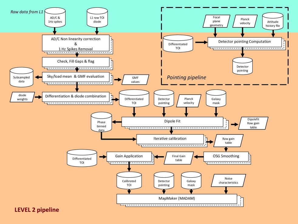
Level 3 collects Level 2 outputs from both HFI (Planck Collaboration VI 2014) and LFI and derives various products such as component-separated maps of astrophysical foregrounds, catalogues of various classes of sources, and the likelihood of various cosmological and astrophysical models given the frequency maps.

4 Time ordered information (TOI) processing

The Level 1 pipeline receives telemetry data as a stream of packets that are handled automatically in several steps:

• uncompress the retrieved packets;

• de-quantize and de-mix the uncompressed packets to retrieve the original signal in analog to digital units (ADU);

• transform ADU data into volts using a conversion factor stored in the packet header;

• cross-correlate time information to time stamp each sample uniquely;

• store the resulting timelines in a database interface to the Level 2 pipeline.

We made no change in Level 1 software during the mission. Detailed information on how each of the steps listed above was applied is provided in Zacchei et al. (2011). To avoid strong gradients in the signal and signals that do not project correctly in the maps, we established the procedure to flag a single scientific sample described in Sect. 4.1.

4.1 Input flags

For each sample we define a 32-bit flag mask to identify potential inconsistencies in the data and to enable the pipeline to skip that sample or handle it differently. The TOI from all LFI detectors are archived in the Level 1 database, and regularly checked to identify and flag events that can affect the scientific analysis. These events include missing or anomalous data, and data acquired during the manoeuvres regularly performed to repoint the telescope according to the Planck scanning strategy. Table 2 summarizes the percentage of time associated with these events for the nominal mission. The table also reports the total percentage of Level 1 TOIs usable in the scientific analysis. Most of the missing data are from telemetry packets in which the arithmetic compression performed by the Science Processing Unit (SPU) is incorrect, causing a decompression error. They are rare, and have negligible impact on the scientific analysis. For instance, for the entire 70 GHz channel, the total amount of missing data corresponds to 130 lost seconds in 15 months. The instrument team performs a daily check of the data retrieved during the daily telecommunication period with the satellite; the data cover an entire operational day (OD). Part of this analysis consists of identifying, for each detector, time windows where either the total power signal or the differentiated signal shows anomalous fluctuations or jumps. Depending on the characteristics of the anomaly identified, a time window can be flagged as unusable for science. Currently, the criteria defined to flag time windows as unusable include:

• gain changes in the data acquisition electronics that cause saturation of the sky or reference load signals;

• abrupt changes in voltage output with slow recovery ($>$1 min), caused by gain fluctuations in the back-end module amplifier, induced by electrical or thermal variations, which generate discontinuities in the differentiated signal;

• short, abrupt changes in voltage output caused by fluctuations in the low noise amplifiers in the front-end module, which produce asymmetries between the sky and reference load signals and possibly first order effects in the differentiated signal;

• permanent changes in the voltage output caused by a permanent change at the front-end module (amplifier bias or focal plane unit temperature) or back-end module (temperature or HEMT gain variations) – in such cases, only a small time window around the discontinuity is flagged as unusable;

• “popcorn” noise on the total power signal of one or both detectors due to variations in the back end diode or in the front end low noise amplifiers, causing short time windows ($<$1 m) of unusable data.

In Table 2, the row labelled “Anomalies” reports the percentage of observation time flagged as unusable for these reasons in the scientific analysis. The almost 1.0 % shown for the 44 GHz channel corresponds to a total time of 113 hours. Finally, the times of manoeuvres and stable pointing periods are recovered from the attitude history files provided by the Planck flight dynamics team. Detector samples corresponding to manoeuvres are flagged so they can be ignored in subsequent steps.

Table 2: Percentage of LFI observation time lost due to missing or unusable data, and to manoeuvres^a.

Category 30 GHz 44 GHz 70 GHz

Missing [%]. 0.00014 0.00023 0.00032

Anomalies [%]. 0.82220 0.99763 0.82925

Manoeuvres [%]. 8.07022 8.07022 8.07022

Usable [%]. 91.10744 90.93191 91.10021

^aThe remaining percentage is used in scientific analysis.

Tasks within the Level 2 pipelines both fill gaps in the data with artificial noise and flag them properly. Other tasks locate transits of planets and other moving objects within the solar system, again flagging samples affected by such observations.

4.2 ADC linearity correction

The ADCs convert the analogue detector voltages to numbers, which are then processed on-board by the radiometer electronics box assembly. Since they are directly involved with the signal power, their linearity is as important as that of the receivers and detectors, with any departure appearing as a distortion in the system power response curve. In differential measurements such as those carried out by the Planck LFI instrument, small localized distortions in this curve can have a large impact, since the calibration factor depends on the gradient of the response curve at the point at which the differential measurements are made. This effect is described in detail in Planck Collaboration III (2014); its impact on calibration is described in Planck Collaboration V (2014).

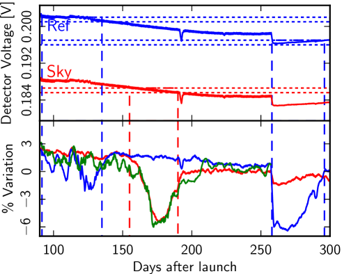
The effect is observed in some LFI radiometer data, appearing as gain variations seen at particular detector voltages. This is shown for the most affected channel, RCA2501, in Fig. 2, where the upper plot shows the measured voltages of the sky and reference loads and the lower plot shows the percentage variations of gain and noise in the sky and reference voltages. The range of the upper plot is matched to that of the lower plot, so for normal gain variations the same pattern should be seen for both. That is clearly not the case. When the sky signal is near 0.186 V, marked by horizontal dotted lines, both the inverse gain and the sky “white noise” estimates show anomalies (the time interval affected is indicated by vertical dashed lines). The same anomalous behavior of the reference white noise signal and inverse gain is seen in two intervals when the reference signal is near 0.197 V and 0.202 V. Outside of these limited ranges, the variations in all plotted signals track one another, such as the feature at day 192 in the sky voltage, or the drop at day 257 when the transponder was turned on permanently.

The response curves can be reconstructed by tracking how the noise amplitude varies with the apparent detector voltage in the TOI. The radiometers are assumed to be stable and the intrinsic thermal noise can be taken to be constant in terms of temperature, so any voltage variations are then assumed to be due to both gain drift and ADC effects. The method for this correction is set out in appendix A of Planck Collaboration III (2014).

Figure 2: Effect of ADC non-linearities on time-ordered data of one 44 GHz diode. The upper plot shows the recorded detector voltages for sky (red) and reference (blue). Voltage ranges affected by ADC non-linearities are marked by horizontal dotted lines. Time ranges affected are marked by vertical dashed lines. The lower plot shows the percentage variation of the inverse of the gain factor from the dipole gain (green) and the “white noise” estimates on the sky and reference voltages (sky red, reference blue). The gain estimates have been smoothed by a three-day moving mean, the noise by a one-day moving mean.

4.3 Corrections for electronic spikes

Electronic spikes in the signal are caused by an interaction between the housekeeping electronics clock and the scientific data line in the on-board data acquisition system. The spikes are synchronous with the on-board time, with no changes in phase over the entire acquisition period, allowing the construction of dedicated templates that are then removed from the timelines. Spikes are present in all frequencies, but are significant only at 44 GHz due to the high gain of these detectors. Consequently, electronic spikes are removed only in this channel. This process and the evaluation of the effect at map level are described in Planck Collaboration III (2014).

4.4 Demodulation: Gain modulation factor estimation and application

Each diode switches at 4096 Hz (Mennella et al. 2010) between the sky and the 4 K reference load. Voltages $V_{\rm sky}$ and $V_{\rm load}$ are dominated by $1/f$ noise, with knee frequencies of tens of hertz. This noise is highly correlated between the two streams, a result of the pseudo-correlation design (Bersanelli et al. 2010), and differencing the streams results in a dramatic reduction of the $1/f$ noise. To force the mean of the difference to zero, the load signal is multiplied by the gain modulation factor (GMF in Fig. 1) $R$, which can be computed in several ways (Mennella et al. 2003). The simplest method, and the one implemented in the processing pipeline, is to take the ratio of DC levels from sky and load outputs obtained by averaging the two time streams, i.e., $R=\langle V_{\rm sky}\rangle/\langle V_{\rm load}\rangle$. Then

$$\Delta V(t)=V_{\rm sky}(t)-\frac{\langle V_{\rm sky}\rangle}{\langle V_{\rm load}\rangle}V_{\rm load}(t)\thinspace.$$ (1)

$R$ is computed from unflagged data for each pointing period and then applied to create the differenced timelines. The $R$ factor has been stable over the mission so far, with overall variations of 0.03–0.04 %. A full discussion regarding the theory of this value is reported in Mennella et al. (2011).

4.5 Combining diodes

The receiver architecture is symmetric, with two complementary detector diodes providing output for each receiver channel. As described in Seiffert et al. (2002) and Mennella et al. (2010), imperfect matching of components limits the isolation between the complementary diodes of the receivers to between $-10$ and $-15$ dB. This imperfect isolation leads to a small anticorrelated component in the white noise. We perform a weighted average of the time-ordered data from the two diodes of each receiver just before the differentiation. This avoids the complication of tracking the anticorrelated white noise throughout the subsequent analysis. We treat the combined diode data as the raw data, and calibration, noise estimation, mapmaking etc. are performed on these combined data. We use inverse noise weights determined from an initial estimate of the calibrated noise for each detector. The weights, reported in Table 3, are kept fixed for the entire mission.

Table 3: Weights used in combining diodes^a.

     Diode

Radiometer      M-00      M-01      S-10      S-11

LFI-18.      0.567      0.433      0.387      0.613

LFI-19.      0.502      0.498      0.551      0.449

LFI-20.      0.523      0.477      0.477      0.523

LFI-21.      0.500      0.500      0.564      0.436

LFI-22.      0.536      0.464      0.554      0.446

LFI-23.      0.508      0.492      0.362      0.638

LFI-24.      0.602      0.398      0.456      0.544

LFI-25.      0.482      0.518      0.370      0.630

LFI-26.      0.593      0.407      0.424      0.576

LFI-27.      0.520      0.480      0.485      0.515

LFI-28.      0.553      0.447      0.468      0.532

^aA perfect instrument would have weights of 0.500 for both diodes.

5 Pointing

Proper pointing reconstruction is critical and has a direct impact in the determination of an accurate photometric calibration. The pointing for each radiometer $\hat{\@vec{P}}_{\mathrm{rad}}(t)$ at time $t$ is given by

$$\hat{\@vec{P}}_{\mathrm{rad}}(t)=\mathcal{R}_{\mathrm{Ecl},\mathrm{Body}}(t)\thinspace\mathcal{R}_{\mathrm{Body},\mathrm{rad}}\hat{\@vec{e}}_{\mathrm{z}}.$$ (2)

The $\mathcal{R}_{\mathrm{Body},\mathrm{rad}}$ matrix encodes the orientation of the beam pattern with respect to the body reference frame defined by the spacecraft structure. We adopt the convention that in the reference frame of the beam, the optical axis is aligned with $\hat{\@vec{e}}_{\mathrm{z}}$. $\mathcal{R}_{\mathrm{Body},\mathrm{rad}}$ is parameterized by a set of rotation angles in the RIMO derived from flight data and ground-based measurements. $\mathcal{R}_{\mathrm{Ecl},\mathrm{Body}}(t)$ is derived by time interpolation of quaternions distributed in the attitude history files, it encodes the orientation of the spacecraft body with respect to the reference frame . The spacecraft attitude is determined from Planck star tracker data, and during periods of stability between maneuvers is sampled at 8 Hz, much lower than the LFI sampling frequency. Equation 2 incorporates a large amount of information on the satellite and a long chain of transformations between reference frames, each one being a possible source of systematic error. Indeed, even a small aberration compared to the beam size can introduce significant photometric effects if the gradient of the temperature field is large enough. The two most important sources of aberration identified and corrected are stellar aberration and the apparent change in wobble angles likely produced by thermal deformations of the star tracker support.

5.1 Stellar aberration

The star tracker system is the basis for the reconstructed astrometric attitude of the Planck spacecraft in the solar system barycentric reference frame; however, the effective pointing direction is affected by stellar aberration due to the orbital motion of Planck and the finite speed of light. In the non-relativistic case, stellar aberration is given by

$$\hat{\@vec{P}}^{\prime}=(\hat{\@vec{P}}+\mathbf{v}_{\mathrm{Planck}}/c)/\left|\hat{\@vec{P}}+\mathbf{v}_{\mathrm{Planck}}/c\right|,$$ (3)

where $\hat{\@vec{P}}^{\prime}$ is the aberrated pointing direction, $\mathbf{v}_{\mathrm{Planck}}$ is the orbital velocity of Planck in the solar system barycentric frame, and $c$ is the speed of light. From this formula, the deflection angle $\delta_{\mathrm{P}}=\arccos(\hat{\@vec{P}}^{\prime}\cdot\hat{\@vec{P}})$ can be derived. Planck moves at about 30 km s^-1 in the ecliptic plane, and scan circles are nearly normal to it. Therefore $\delta_{\mathrm{P}}\leq 20.6$^′′, and the greatest deflection occurs near the ecliptic poles. If left uncorrected, this aberration would distort the maps, producing a seasonal shift near the equator and a blurring near the ecliptic poles. Accurate simulations show that the distortion radius is maximal at the ecliptic poles, $(l_{\mathrm{Gal}},b_{\mathrm{Gal}})=(96$ .${}^{\circ}384,29$ .${}^{\circ}811)$ and $(276$ .${}^{\circ}384,-29$ .${}^{\circ}811)$, and that it decreases towards the ecliptic down to a minimum of about 0 .^∘1 on the ecliptic. The boundary of the region in which the distortion radius is at least half the polar value is roughly a ring centred on the poles, with radius about $60^{\circ}$. There are some variations in the radius and in the longitudinal shape of the boundary, both smaller than a few degrees, due to the scanning strategy, and also to the different angular distances from the spin axis of the various feedhorns.

5.2 Wobble angles

Wobble angles describe the unavoidable misalignment of the body reference frame with respect to the reference frame defined by the satellite principal inertial axis. The nominal spin axis for the satellite is nearly 0 .^∘5 away from the principal moment of inertia, and the effective scan circles are about half a degree smaller than the nominal ones (Planck Collaboration I 2011). Wobble angles and their variations in time, either real or apparent, are measured by careful modelling of the observed Planck attitude dynamics included in the attitude history files. Planck Collaboration I (2011) reported an apparent variation of the wobble angles likely produced by thermoelastic deformations that change the relative orientation of the star tracker with respect to the body reference frame. The change was detected in scans of Jupiter. Since this variation is rigidly transported by the rotations of spacecraft body, its effect will be largely averaged out near the poles and will be maximal near the ecliptic, the opposite of the stellar aberration effect.

Of the three angles that describe the wobble, $\psi_{1}$ has largely negligible effects and $\psi_{3}$ is badly determined, so the LFI pipeline corrects only for variations in $\psi_{2}$, whose effect is apparent changes of the angular distance between the telescope and the spin axis. Typical changes of this angle are equivalent to apparent changes of scan circle radii of $\pm 0\hbox{\hbox to0.0pt{.\hss}\kern 0.80002pt}^{\scriptstyle\prime}\hbox{\kern-0.29999pt}1$, giving equivalent displacements in pointing between consecutive surveys of $0\hbox{\hbox to0.0pt{.\hss}\kern 0.80002pt}^{\scriptstyle\prime}\hbox{\kern-0.29999pt}2$.

6 Main beams and the geometrical calibration of the focal plane

The profiles and locations of the beams are determined from the four observations of Jupiter listed in Table 4, following the procedure described in Zacchei et al. (2011) and Mennella et al. (2011). Details are given in Planck Collaboration IV (2014). The origin of the focal plane is the optical line of sight defined in Tauber et al. (2010). The LFI beam centers are given by four numbers, $\theta_{uv}$, $\phi_{uv}$, $\psi_{\mathrm{u}v}$, and $\psi_{\rm pol}$ (see Planck Collaboration 2013 for the definitions of these angles). Only $\theta_{uv}$ and $\phi_{uv}$, which are the beam pointing in spherical coordinates referred to the line of sight, can be determined with Jupiter observations. The polarization orientation of the beams, defined by $\psi_{uv}+\psi_{\rm pol}$, is not estimated from flight data but is derived from main beam simulations based on ground measurements.

Table 4: Approximate dates of the Jupiter observations^a.

Jupiter transit Date OD Scan 1 (J1). 21/10/2009 – 05/11/2009 161 – 176 Scan 2 (J2). 27/06/2010 – 12/07/2010 410 – 425 Scan 3 (J3). 03/12/2010 – 18/12/2010 569 – 584 Scan 4 (J4). 30/07/2011 – 08/08/2011 808 – 817

^aThe periods include the scan by the entire LFI field of view.

For each beam, the pointing is determined by the location of the maximum of an elliptical Gaussian fit to that beam. This was done for each beam in each single scan. Results are reported, with errors, in Planck Collaboration IV (2014).

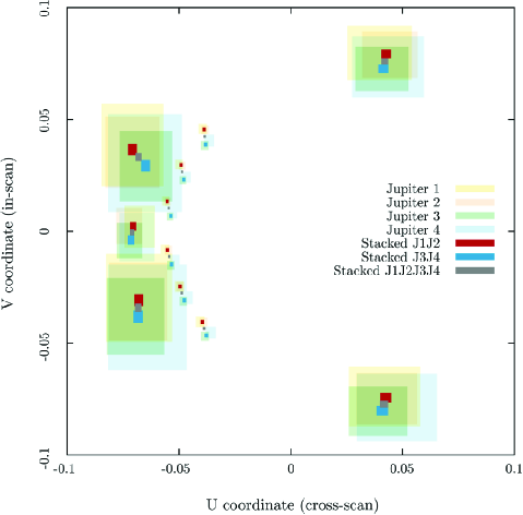
In addition, the beams are stacked in pairs (J1J2 and J3J4) and all together (J1J2J3J4) in order to improve the signal-to-noise ratio of the measurements. Before the stacking, each beam is artificially repointed along the direction given by the arithmetic average of the center of each beam to be stacked. Then a fit is performed again on the stacked beams and the resulting parameters recorded. For single scans it has been found that there is an agreement within $2$^′′ in the pointing direction between J1 and J2. The same agreement occurs between J3 and J4. In contrast, a $\sim 15$^′′ systematic deviation of the beam center was detected when comparing J1J2 to J3J4. Figure 3 shows the reconstructed beam positions and errors in the line-of-sight frame magnified by a factor of 100. The shift is evident for the 70 GHz beams, as well as in all the J1J2 and J3J4 stacked beam centers. The change in the location has been found mainly in the scan direction (i.e., $v$-coordinate). To account for this pointing shift, we apply two pointing solutions for LFI. The first focal plane calibration is valid from OD91 to OD540 and is based on the J1J2 beam pointing determination. The second calibration is valid from OD541 to OD563 and is based on the J3J4 beam pointing calibration. The reconstructed angles are reported in Table 5.

Figure 3: Main beam pointing directions measured with the first four Jupiter crossings. Single scans are yellow, light red, green, and light blue. First and second stacked scans are red, third and fourth stacked scans are blue, and four stacked scans are grey. The colored boxes refer to the measured uncertainties magnified by a factor of 100. The differences in pointing were normalized to the J1 measurements, and were magnified by the same factor of 100. The $U$ and $V$ axis are defined as $U=\sin(\theta)\cos(\phi)$ and $V=\sin(\theta)\sin(\phi)$, where $\theta$ and $\phi$ are the angle respect the LOS (line of sight) defined in Tauber et al. (2010).

Table 5: Focal plane geometry

Radiometer      $$\theta_{uv}$$^{a a        b b      c c}

LFI-18S.      3.334 131.803        3.335 131.752      22.2 0.0

LFI-18M.      3.333 131.812        3.335 131.759      22.2 90.2

LFI-19S.      3.208 150.472        3.209 150.408      22.4 0.0

LFI-19M.      3.208 150.467        3.209 150.402      22.4 90.0

LFI-20S.      3.183 168.189        3.183 168.121      22.4 0.0

LFI-20M.      3.183 168.178        3.183 168.109      22.4 89.9

LFI-21S.      3.184 169.265        3.182 169.324      22.4 0.0

LFI-21M.      3.184 169.274        3.183 169.336      22.4 90.1

LFI-22S.      3.172 151.352        3.170 151.405      22.4 0.1

LFI-22M.      3.172 151.345        3.170 151.398      22.4 90.1

LFI-23S.      3.280 132.255        3.277 132.287      22.1 0.0

LFI-23M.      3.280 132.234        3.277 132.274      22.1 89.7

LFI-24S.      4.070 179.506        4.069 179.449      0.0 0.0

LFI-24M.      4.070 179.538        4.071 179.488      0.0 90.0

LFI-25S.      4.984 61.105        4.981 61.084      113.2 0.0

LFI-25M.      4.985 61.065        4.981 61.051      113.2 89.5

LFI-26S.      5.037 61.662        5.040 61.669      113.2 0.0

LFI-26M.      5.037 61.649        5.040 61.676      113.2 90.5

LFI-27S.      4.343 153.958        4.343 154.033      22.3 0.0

LFI-27M.      4.345 153.981        4.341 154.010      22.3 89.7

LFI-28S.      4.374 153.413        4.376 153.369      22.3 0.0

LFI-28M.      4.374 153.419        4.376 153.371      22.3 90.3

^aBeam pointing reconstructed using the first two Jupiter transits (J1 and J2).

^bBeam pointing reconstructed using the last two Jupiter transits (J3 and J4).

^cPolarization orientation of the beam measured during ground test.

6.1 Scanning beams

Scanning beams are defined as the beams measured in flight on planets. The scanning beam derives from the optical beam coupled with the radiometer response, and smeared by the satellite motion. With four Jupiter transit measurements we were able to reconstruct the beam shape down to $-20$ dB from the peak at $30$ and $44$ GHz, and down to $-25$ dB at $70$ GHz. From the beam shape we estimated the main beam parameters using a bivariate Gaussian fit on the four stacked beams (J1J2J3J4). The fitting procedure, described in Zacchei et al. (2011), was slightly modified to correct for offsets in the data and to avoid noise contamination. We refer to the companion paper on LFI beams (Planck Collaboration IV 2014) for details on procedures and results. Table 6 gives the average values of the FWHM and ellipticity, with errors.

Table 6: LFI beam FWHM and ellipticity measured in flight from four Jupiter passes^a.

      FWHM^b Beam       $$[\rm arcmin] 13.44\pm 0.03 1.26\pm 0.01 13.11\pm 0.04 1.27\pm 0.01 12.84\pm 0.04 1.28\pm 0.01 12.81\pm 0.03 1.29\pm 0.01 12.95\pm 0.03 1.28\pm 0.01 13.33\pm 0.04 1.26\pm 0.01 23.17\pm 0.07 1.37\pm 0.01 30.60\pm 0.10 1.19\pm 0.01 30.49\pm 0.12 1.20\pm 0.01 33.09\pm 0.11 1.38\pm 0.01 33.23\pm 0.11 1.37\pm 0.01$$       Ellipticity^c 70 GHz mean.       13.08       1.27       LFI-18 .                     LFI-19 .                     LFI-20 .                     LFI-21 .                     LFI-22 .                     LFI-23 .               44 GHz mean.       28.09       1.25       LFI-24.                     LFI-25.                     LFI-26.               30 GHz mean.       33.16       1.37       LFI-27.                     LFI-28.              

^aUncertainties are the standard deviation of the mean of the $$1\sigma$$ statistical uncertainties of the fit. A small difference is expected between the M and S beams, caused by optics and receiver non-idealities.

^bThe square root of the product of the major axis and minor axis FWHMs of the individual horn beams, averaged between M and S radiometers.

^cRatio of the major and minor axes of the fitted elliptical Gaussian.

6.2 Effective beams

The effective beam at a given pixel in a map of the sky is the average of all scanning beams that observed that pixel during the observing period of the map given the Planck scan strategy. We compute the effective beam at each LFI frequency scanning beam and scan history in real space using the FEBeCoP (Mitra et al. 2011) method. Details of the application of FEBeCoP to Planck data will be discussed in a future paper. Effective beams were used to calculate the effective beam window function as reported in Planck Collaboration IV (2014) and in the source detection pipeline necessary to generate the PCCS catalogue  (Planck Collaboration XXVIII 2014). Table 7 lists the mean and rms variation across the sky of the main parameters computed with FEBeCoP. Note that the FWHM and ellipticity in Table 7 differ slightly from the values reported in Table 6. This results from the different way in which the Gaussian fit was applied. The scanning beam fit was determined by fitting the profile of Jupiter on timelines and limiting the fit to the data with signal-to-noise ratio greater than 3, while the fit of the effective beam was computed on GRASP maps projected in several positions of the sky  (Planck Collaboration IV 2014). The latter are less affected by the noise.

Table 7: Mean and rms variation across the sky of FWHM, ellipticity, orientation, and solid angle of the FEBeCop effective beams computed with the GRASP beam fitted scanning beams^a.

Frequency      FWHM [arcmin]      $$e$$                  FWHM_eff

70.                              13.31

44.                              27.12

30.                              32.24

^aFWHM_eff is the effective FWHM estimated from the main beam solid angle of the effective beam, $$\Omega_{\mathrm{eff}}={\mathrm{mean}}(\Omega)$$.

7 Photometric calibration

Conversion of time-ordered streams of voltages into time-ordered streams of thermodynamic temperatures is modelled by

$$V=G\times\bigl{(}T_{\mathrm{sky}}+T_{\mathrm{noise}}\bigr{)},$$ (4)

where $V$ is the voltage measured by the ADC, $T_{\mathrm{sky}}$ is obtained by convolving the sky temperature with the beam response of the instrument at a given time, and $T_{\mathrm{noise}}$ is the noise temperature of the radiometer. In general, we are interested in $K=G^{-1}$, as the purpose of the calibration is to convert $V$ back into a temperature. As described in Planck Collaboration V (2014), two different algorithms are used for calibrating the LFI radiometers in this data release:

1. For the 44 and 70 GHz radiometers, we use a technique called optimal search of gain, which is similar to the one used by WMAP (Hinshaw et al. 2009). It is based on fitting the radiometric signal to the expected dipolar anisotropy induced by the motion of the spacecraft with respect to the CMB rest frame.

2. For the 30 GHz radiometers, we use a technique that combines the knowledge of the dipolar anisotropy (as above), then additionally takes into account the observed fluctuations in the measurement of the signal of the 4 K reference loads.

The overall accuracy in the calibration is reported in Table 1. The reasons why we used two different algorithms are discussed in Planck Collaboration V (2014). We describe the algorithms in the following sections.

7.1 Iterative calibration

The main features of the iterative calibration algorithm used for 44 and 70 GHz are the following:

1. We combine the speed of the spacecraft with respect to the Sun, $\@vec{v}_{\mathrm{Planck}}$, and the speed of the Sun with respect to the CMB, $\@vec{v}_{\mathrm{Sun}}$. The angle between the velocity vector and the axis of the relevant beam is $\theta$. The dipole is then evaluated considering the relativistic correction

   $$\Delta T=T_{\mathrm{CMB}}\left(\frac{1}{\gamma(1-\beta\cos\theta)}-1\right),$$ (5)

   where $T_{\mathrm{CMB}}=2.7255\thinspace\mathrm{K}$. We produce discrete time ordered data (TOD) of the expected overall dipole signal for each sample in a pointing period.

2. Using pointing information, we project both $V_{i}$ and $\Delta T_{i}$ on a HEALPix map ($N_{\rm side}=256$). Multiple hits on the same pixels are averaged. The result is a pair of maps, $V^{\mathrm{map}}_{k}$ and $\Delta T^{\mathrm{map}}_{k}$, with $k$ being the pixel index.

3. We use weighted least squares to estimate $K=G^{-1}$ in Eq. 4 from the correlation between the signal in volts, $V^{\mathrm{sky}}_{k}$, and $\Delta T^{\mathrm{sky}}_{k}$:

   $$V^{\mathrm{map}}_{k}=K^{\mathrm{dip}}\thinspace\Delta T^{\mathrm{map}}_{k}+\epsilon,$$ (6)

   where $K$ and $\epsilon$ are the parameters used in the fit. Each sample $k$ is weighted according to the number of hits per pixel. In computing the fit, we use a frequency-dependent mask to avoid those pixels where a strong non-Gaussian signal other than the dipole is expected, i.e., point sources and the Galaxy.

4. The main source of uncertainties in the fit using the dipole is the cosmological CMB signal itself. To improve the result, we calibrate the data using $K_{i}$ and $\epsilon_{i}$, remove the dipole convolved with the beam, and make a map, which represents an estimation of the cosmological signal. To reduce the effect of noise, we combine data streams from both radiometers of the same horn. Then we remove the estimated cosmological signal from the data, make a map using a simplified destriping algorithm, and use the results to refine the values of $K_{i}$ and $\epsilon_{i}$. We iterate the procedure until convergence. The result of this process is a set of gains, $K^{\mathrm{iter}}_{i}$, and offsets, $\epsilon^{\mathrm{iter}}_{i}$.

5. An adaptive low-pass filter based on wavelets is applied to the vectors $K^{\mathrm{iter}}_{i}$ and $\epsilon^{\mathrm{iter}}_{i}$ to reduce high-frequency noise, particularly near the regions where the spacecraft is unfavorably aligned with the dipole.

7.2 Calibration using 4K reference load signal

To calibrate the 30 GHz radiometers, we used a different calibration scheme based on the signal measuring the temperature of the 4 K reference loads. This calibration has the advantage of being less dependent on optical systematics such as far sidelobes (Planck Collaboration III 2014), at the expense of being more sensitive to systematics in the radiometers such as ADC non-linearities (Planck Collaboration V 2014). The algorithm can be summarized as follows:

1. For each pointing period $i$, a set of gains $K^{\mathrm{iter}}_{i}$ is estimated using the iterative procedure described in Sect. 7.1.

2. The values of $K^{\mathrm{iter}}_{i}$ are used to estimate the value of the constant $K_{0}$ in the equation

   $$K^{\mathrm{iter}}_{i}=K_{0}\times\left(2-\frac{V^{\mathrm{ref}}_{i}}{V^{\mathrm{ref}}_{0}}\right),$$ (7)

   where $V^{\mathrm{ref}}_{i}$ is the average value of the 4 K reference load signal (in volts) over the $i$-th pointing period, and $V^{\mathrm{ref}}_{0}=\langle V^{\mathrm{ref}}_{i}\rangle$ is a voltage representative of the value of $V^{\mathrm{ref}}_{i}$ over the whole mission. The constant $K_{0}$ is estimated using a weighted, one-parameter, linear least squares fit, where the weights are chosen to be proportional to the expected amplitude of the dipole-like signal in the sky, $\Delta T^{\mathrm{dip}}_{i}$, at the $i$-th pointing.

3. Using the value of $K_{0}$ estimated in the previous point, we extract a new set of gains $K^{\mathrm{4,\mathrm{K}}}_{i}$ with the equation

   $$K^{4\thinspace{\rm K}}_{i}\equiv K_{0}\times\left(2-\frac{V^{\mathrm{ref}}_{i}}{V^{\mathrm{ref}}_{0}}\right).$$ (8)

The procedure can be modelled by the following GNU R code:

data<-data.frame(gain = iterative.dipole.gains,
                 vref = 2 - signal.4K/mean(signal.4K),
                 dipole = dipole.amplitude.KCMB)
fit<-lm(gain ~ vref + 0, data, weights = dipole)
gains.4K <- fit$coefficients[1] * data$dvref

where iterative.dipole.gains, signal.4K, and dipole.amplitude.KCMB are three vectors containing the iterative gains $K^{\mathrm{iter}}_{i}$ before the smoothing filter, the 4 K reference load signal $V^{\mathrm{ref}}_{i}$ averaged over each pointing period, and the values of $\Delta T_{i}$ (Eq. 5), respectively.

Unlike the procedure in Sect. 7.1, in this case there is no need to smooth the stream of gains, as they share the stability of the voltages $V^{\mathrm{ref}}_{i}$.

7.3 Color correction

Table 8 gives color corrections calculated following the method given in Planck Collaboration V (2014). Values for intermediate spectral indices can be derived by interpolation. The data release includes the UcCC IDL package used by both LFI and HFI (Planck Collaboration IX 2014) that calculates color corrections and unit conversions using the band-averaged bandpass stored in the reduced instrument model (RIMO) file, which is also included in the data release.

Table 8: Multiplicative color corrections cc$(\alpha)$ for individual LFI Radiometer Chain Assemblies and for the band average maps.

Spectral index $$\alpha -2.0 -1.5 -1.0 -0.5 0.0 0.5 1.0 1.5 2.0 2.5 3.0 3.5 4.0 0.938 0.951 0.963 0.973 0.982 0.988 0.994 0.997 0.999 0.999 0.998 0.995 0.991 0.948 0.961 0.972 0.981 0.988 0.994 0.997 0.998 0.997 0.995 0.990 0.983 0.975 0.856 0.878 0.899 0.919 0.939 0.957 0.975 0.991 1.006 1.020 1.032 1.043 1.053 0.889 0.908 0.925 0.941 0.956 0.970 0.983 0.994 1.003 1.011 1.018 1.023 1.027 0.917 0.933 0.947 0.960 0.971 0.981 0.989 0.996 1.001 1.004 1.006 1.006 1.004 1.024 1.026 1.027 1.026 1.023 1.018 1.011 1.003 0.993 0.982 0.969 0.955 0.940 0.985 0.991 0.996 0.999 1.001 1.002 1.002 1.000 0.997 0.993 0.988 0.982 0.975 0.968 0.975 0.981 0.986 0.990 0.994 0.997 0.999 1.000 1.000 0.999 0.998 0.995 0.978 0.984 0.988 0.993 0.996 0.998 0.999 1.000 0.999 0.998 0.996 0.993 0.989 0.967 0.974 0.980 0.985 0.990 0.994 0.996 0.999 1.000 1.000 1.000 0.999 0.997 0.957 0.966 0.973 0.980 0.985 0.990 0.995 0.998 1.000 1.001 1.002 1.002 1.000 0.947 0.959 0.969 0.977 0.985 0.991 0.995 0.998 1.000 1.000 0.998 0.994 0.989 0.948 0.959 0.969 0.978 0.985 0.991 0.995 0.998 1.000 1.000 0.998 0.995 0.991 0.946 0.958 0.968 0.977 0.985 0.991 0.996 0.998 1.000 0.999 0.997 0.993 0.988$$ Horn 70 GHz mean.       LFI-18.       LFI-19.       LFI-20.       LFI-21.       LFI-22.       LFI-23. 44 GHz mean.       LFI-24.       LFI-25.       LFI-26. 30 GHz mean.       LFI-27.       LFI-28.

8 Noise estimation

The estimation of noise properties is fundamental in several aspects of the data analysis. For instance, such measurements are used in the Monte Carlo simulations of noise necessary for power spectrum estimation, as well as to determine proper horn weights to be employed during the map-making process. In addition, inspection of noise properties throughout the mission lifetime is of paramount importance in tracking possible variations and anomalies in instrument performance. Our noise estimation pipeline has been improved over the log-periodogram approach used in Zacchei et al. (2011) by the implementation of a Markov chain Monte Carlo (MCMC) approach for the extraction of basic noise parameters. This allows for an unbiased estimate of the parameters that characterize the non-white noise.

We write the noise spectrum as

$$P(f)=\sigma^{2}\left[1+\left(\frac{f}{f_{\mathrm{knee}}}\right)^{\beta}\right]\thinspace,$$ (9)

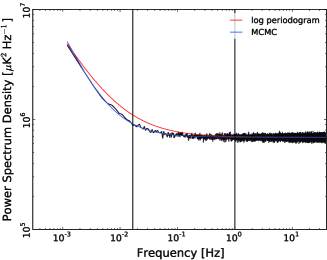
where $\sigma^{2}$ is the white noise level, and $f_{\rm knee}$ and $\beta$ characterize the non-white noise. As before, $\sigma^{2}$ is calculated as the mean of the noise spectrum over the flat, high-frequency tail (see Figs. 4 and 5), typically over the highest 10% of frequency bins shown in the figures. For the 30 GHz radiometers, which have $f_{\rm knee}\approx 100$ mHz, a smaller percentage must be used to get an unbiased estimation. Once white noise is computed, the code creates Markov chains for the other parameters. We get the expected value and variance of each noise parameter from the chain distribution, ignoring the burn-in period.

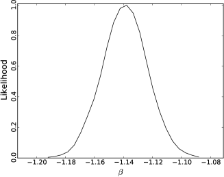
The left panel of Fig. 4 shows a typical spectrum at 70 GHz with the old log-periodogram fit (red line) and the new MCMC-derived spectrum (blue line) superimposed. The center and right panels show the distributions of knee-frequency and slope from the MCMC chains.

Figure 4: Left: Typical noise spectrum at 70 GHz, with “old” log-periodogram fit (red line) and “new” MCMC fit (blue line). Vertical lines mark the frequencies corresponding to the spin period ($1/60$ Hz) and the baseline used in mapmaking ($1$ Hz). The corresponding distributions of knee-frequency and slope from the MCMC chains are shown in the center and right panels, respectively. for the example spectrum.

8.1 Updated noise properties

Radiometer noise properties have been evaluated using the new MCMC just described. We select calibrated radiometer data in periods of five days, and compute noise spectra with the roma iterative generalized least squares map-making algorithm (Natoli et al. 2001; de Gasperis et al. 2005; Prunet et al. 2001; Zacchei et al. 2011). The output is a frequency spectrum to which the new MCMC code is applied. Results at radiometer level on white noise sensitivity are reported in Table 9, while Table 10 shows $1/f$ noise parameters. These are computed taking the median of the ten estimates made for different time ranges over the nominal mission.

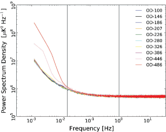
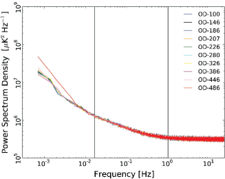
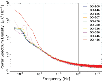
Time variations of the noise properties provide a valuable diagnostic of possible changes in the instrument behavior. The switchover between the two sorption coolers provides an example. Variations in noise properties driven by temperature changes were expected as the performance of the first cooler degraded with time, as well as at the switchover to the redundant cooler. Figure 5 shows noise frequency spectra for radiometers LFI28M, LFI24S, and LFI18M for the nominal mission. White noise levels are stable within $0.5$%. Knee frequencies and slopes are also quite stable until OD 326, after which the spectra show increasing noise and two slopes for the low-frequency part. The latter becomes more evident for spectra around OD 366 and OD 466, when the first cooler starts to be less effective and produces low-frequency thermal noise. This behavior is present at some level in all radiometers, but with different trends, ranging from the small effect shown by LFI24S to more prominent effects as shown by LFI28M and LFI18M.

Figure 5: Time behaviour of noise spectra on selected periods for radiometers 18M (70 GHz, left), 24S (44 GHz, centre), and 28M (30 GHz, right). White noise and $1/f$ noise are constant within $0.5$% until OD 326, after which degradation of the sorption cooler and the switchover to the redundant cooler introduce higher thermal noise at the lowest frequencies. Vertical lines mark the frequencies corresponding to the spin period ($1/60$ Hz) and the baseline used in the mapmaking ($1$ Hz).

Table 9: White noise sensitivities for the LFI radiometers.

     White Noise Sensitivity

     Radiometer M      Radiometer S

     [$$\thinspace\mu\mathrm{K}_{\rm CMB}\thinspace\mathrm{s}^{1/2}$$]      []

70 GHz

      LFI-18 .      511.71.7      466.31.7

      LFI-19 .      579.81.6      554.11.6

      LFI-20 .      587.51.4      619.72.1

      LFI-21 .      451.61.7      560.91.7

      LFI-22 .      489.91.5      531.02.1

      LFI-23 .      503.41.8      538.81.9

44 GHz

      LFI-24 .      461.01.3      398.21.3

      LFI-25 .      413.51.5      393.33.0

      LFI-26 .      480.81.5      419.11.9

30 GHz

      LFI-27 .      282.22.1      304.72.0

      LFI-28 .      318.21.9      286.82.1

Table 10: Knee frequency and slope for the LFI radiometers.

     Knee Frequency $$f_{\rm knee}$$ [mHz]      Slope

     Radiometer M      Radiometer S      Radiometer M      Radiometer S

70 GHz

      LFI-18 .      15.32.8      18.31.6            

      LFI-19 .      11.91.3      14.61.1            

      LFI-20 .      8.41.9      6.01.7            

      LFI-21 .      39.34.0      14.02.4            

      LFI-22 .      10.12.1      15.97.1            

      LFI-23 .      30.21.4      58.89.0            

44 GHz

      LFI-24 .      26.91.2      73.07.9            

      LFI-25 .      20.10.6      46.11.8            

      LFI-26 .      64.42.0      43.88.9            

30 GHz

      LFI-27 .      175.12.2      109.62.3            

      LFI-28 .      127.93.8      43.92.2            

9 Mapmaking

The mapmaking pipeline was described in detail in Zacchei et al. (2011). Here we give an overview, reporting significant updates.

9.1 MADAM pipeline for frequency maps

Frequency maps were produced by the Madam mapmaking code (Keihänen et al. 2010), which takes as input calibrated TOD and corresponding radiometer pointing data in the form of three Euler angles ($\theta,\phi,\psi$). The output consists of three pixelized Stokes maps (T,Q,U) representing the temperature and polarization anisotropies of the observed sky.

The algorithm is based on the destriping technique, where the correlated noise component is modelled by a sequence of offsets, or baselines. The amplitudes of these baselines are determined through maximum-likelihood analysis. Higher-frequency noise, which is not captured by the baseline model, is assumed to be white.

The noise model can be written as

$$n^{\prime}=Fa+n\thinspace,$$ (10)

where $n^{\prime}$ is the total noise stream, $n$ is white noise, $a$ is a vector consisting of the baselines, and $F$ is a matrix of ones and zeros that spreads the baselines into a time-ordered data stream.

Unlike conventional destriping, Madam also uses information on the known noise properties, in the form of a noise prior. This allows extension of the destriping approach to shorter baseline lengths, well below the scanning period of 1 minute.

The baseline length is a key parameter in the destriping technique. We chose the baseline length to be an integral number of samples near 1 s, specifically, 33, 47, and 79 samples for 30, 44, and 70 GHz, respectively, corresponding to 1.0151, 1.0098, and 1.0029 s.

A baseline length of one second is a reasonable compromise between computational burden and the quality of the final map. Shortening the baseline below one second has very little effect on the residual noise.

When mapmaking is run with a short baseline, the noise prior plays an important role. There are not enough crossing points between the one-second data sections to determine the baselines without additional constraints. In this case, the additional constraints are noise priors constructed from the parametrized noise model (Eq. 9) using the values given in Tables 9 and 10. From these we compute the expected covariance between the noise baselines, $C_{a}=\langle aa^{\mathrm{T}}\rangle$. The exact derivation is given in Keihänen et al. (2010). Another important role of the noise prior is to suppress the signal error, which would otherwise increase rapidly with decreasing baseline length. Flagged data sections are handled by setting the white noise variance to infinity for those samples, but not altering the baseline pattern. The flagged samples thus do not contribute to the final map in any way other than serving as place-holders to maintain the time sequence. This is essential for the noise prior to be applied correctly.

The use of a priori information has the danger of hiding problems in the data, since the prior may drive the solution to a correct-looking result, even if the data alone are not in complete agreement with it. To avoid this pitfall, we compute for comparison a subset of the maps with a one-minute baseline without using a noise prior, and compared the maps visually. No artefacts could be seen in either of the maps. Although this is not a quantitative test, similar sanity checks had helped to reveal bugs at earlier stages of the development of the data processing pipeline.

Each data sample is assigned entirely to the pixel in which the center of the beam falls. We used resolution $N_{\rm side}=1024$ for all frequencies. The average width of one pixel at this resolution is 3.^′5, which may be compared to the FWHM of the beams at each frequency given in Table 1. For the nominal mission, every pixel is observed for the 70 GHz channel; however, at 30 GHz and 44 GHz, where the sampling frequency is lower, there remain individual pixels that are unobserved, or observed with insufficient polarization angle coverage to recover the polarization. These are marked by a special value in the product maps. In the 30 GHz map there are 158 such pixels, while in the 44 GHz frequency map there are 250 (0.0013 % and 0.0020 %, respectively).

The maximum likelihood analysis that lies behind our mapmaking algorithm and the derivation of the destriping solution are presented in Keihänen et al. (2010). Here we quote the most important formulas for easier reference.

The vector of baseline $a$ is solved from the linear equation

$$\left(F^{\mathrm{T}}C_{w}^{-1}ZF+C_{a}^{-1}\right)\thinspace a=F^{\mathrm{T}}C_{w}^{-1}Z\thinspace y\thinspace,$$ (11)

where $C_{a}$ and $C_{w}$ are covariance matrices that represent the a priori known properties of the baselines and the white noise component, respectively, $y$ is the observed data stream, and

$$Z=I-\left(P^{\mathrm{T}}C_{w}^{-1}P\right)^{-1}P^{\mathrm{T}}C_{w}^{-1}\thinspace,$$ (12)

where $P$ is the pointing matrix, which picks values from the T,Q,U maps and spreads them into time-ordered data.

The final map is then constructed as

$$m=\left(P^{\mathrm{T}}C_{w}^{-1}P\right)^{-1}P^{\mathrm{T}}C_{w}^{-1}(y-Fa)\thinspace.$$ (13)

The white noise component is assumed to be uncorrelated, but not necessarily with uniform variance. Matrix $C_{w}$ is thus diagonal, but not constant.

Matrices $P$, $F$, and $C_{w}$ are large, but sparse. They are not constructed explicitly, rather, the operations represented formally as matrix multiplication above are performed algorithmically. For instance, multiplication by $P^{T}$ represents an operation where the time-ordered data are coadded on a sky map.

We solve Eq. 11 through conjugate gradient iteration. Convergence is reached typically after 20 to 100 iterations, depending on the sky coverage and radiometer combination. Full mission maps, where the whole sky is covered, typically converge faster than single-survey maps, where sky coverage is incomplete.

The observed signal can be written as

$$y_{i}=T(\omega_{i})+Q(\omega_{i})\cos(2\psi_{i})+U(\omega_{i})\sin(2\psi_{i})\thinspace,$$ (14)

where $\omega_{i}$ is the sky pixel to which the sample is assigned and $\psi_{i}$ defines the beam orientation. The elements of the pointing matrix $P$ consist of ones and cosine and sine factors picked from this equation.

When constructing single-horn maps, we include only the temperature component of the sky into the computation. In the case of frequency or horn-pair maps, we include the $I$, $Q$, and $U$ Stokes components, although only the $I$ component maps are included in the 2013 data release.

We deviate from the formulation of the original Madam paper in that we have written $C_{w}$ in place of $C_{n}$. This reflects the fact that the $C_{w}$ matrix is not necessarily the white noise covariance, but rather a user-defined weighting factor. We diverge from the maximum-likelihood noise-weighted solution in order to have better control over polarization systematics. Specifically, the weight for a given horn is taken to be

$$C_{w}^{-1}=\frac{2}{\sigma_{\mathrm{M}}^{2}+\sigma_{\mathrm{S}}^{2}}\thinspace,$$ (15)

where $\sigma_{M}$ and $\sigma_{S}$ are the white noise sensitivities of the two radiometers of the horn, computed from the values given in Table 9. The weights are identical for radiometers of same horn. The formula above is applied for non-flagged samples. For flagged samples we set $C_{w}^{-1}=0$. With this horn-uniform weighting, polarization maps become dependent solely on the signal difference between M and S radiometers, apart from a small leakage due to the fact that the polarization sensitivities are not exactly at 90^∘ from each other. Many systematic effects, which are equal or strongly correlated within a horn, cancel out in the difference. Horn-uniform weighting has the benefit of reducing spurious polarization signals arising from beam shape mismatch, since the beam shapes of a radiometer pair sharing a horn are typically quite similar (though not identical). Complete cancellation also requires that the same flags be applied to both data streams. Therefore, if a sample for one radiometer is flagged, we discard the corresponding sample for the other radiometer as well.

The covariance of residual white noise in the map solution is obtained from

$$C_{\mathrm{wn}}=\left(P^{\mathrm{T}}C_{w}^{-1}P\right)^{-1}P^{\mathrm{T}}C_{w}^{-1}C_{n}C_{w}^{-1}P\left(P^{\mathrm{T}}C_{w}^{-1}P\right)^{-1}\thinspace,$$ (16)

where now $C_{n}$ is the actual white noise covariance of the time-ordered data. For a given $C_{n}$, the residual noise would be minimized when $C_{w}=C_{n}$, in which case $C_{\mathrm{wn}}=\left(P^{\mathrm{T}}C_{n}^{-1}P\right)^{-1}$. In using a different weighting, we accept slightly higher noise in return for better removal of systematics.

Altering matrix $C_{w}$ does not bias the solution, as may be verified by inserting $y=Pm$ in the solution above. It merely affects the level of residual noise.

The white noise covariance only takes into account the uncorrelated component of the noise. The computation of a full noise covariance matrix, which also captures the residual correlated noise, is discussed in Sect. 9.2.2.

The destriping solution assumes that the sky signal is uniform within one pixel. This is not strictly true, which gives rise to the signal error: signal differences within a pixel are falsely interpreted as noise, which leads to spurious striping, especially in the vicinity of point sources or in other regions where the signal gradient is large. Most of this effect is seen where Galactic emission is strong.

Similarly, mismatch in frequency response between radiometers gives rise to spurious striping, as different radiometers record slightly different signals from the same source. In this case also, the main effect is seen where Galactic emission is strong.

To reduce these undesired effects, we mask the strongest Galactic region and compact sources in the destriping process and use crossing points of rings only outside the masked region to solve the noise baselines. The masks for 30, 44, and 70 GHz leave 78.7%, 89.4%, and 89.7% of the sky, respectively, included in the analysis. Some of the baselines fall completely inside the masked region, but can still be recovered with reasonable accuracy with help of combined information of the neighbouring baselines and the noise prior.

Table 11 lists the delivered maps. All have HEALPix resolution $N_{\rm side}=1024$.

Table 11: Released LFI maps.

Map      Horns      OD range      Baseline (s)      Sky coverage (%)

30 GHz nominal.      27, 28      91–563      1.0151      99.999

30 GHz survey 1.      27, 28      91–270      1.0151      97.205

30 GHz survey 2.      27, 28      270–456      1.0151      97.484

44 GHz nominal.      24, 25, 26      91–563      1.0098      99.998

44 GHz survey 1.      24, 25, 26      91–270      1.0098      93.934

44 GHz survey 2.      24, 25, 26      270–456      1.0098      93.310

70 GHz nominal.      18, 19, 20, 21, 22, 23      91–563      1.0029      100.000

70 GHz survey 1.      18, 19, 20, 21, 22, 23      91–270      1.0029      97.938

70 GHz survey 2.      18, 19, 20, 21, 22, 23      270–456      1.0029      97.474

9.2 Low-resolution data set

To fully exploit the information contained in the large scale structure of the microwave sky, pixel-pixel covariances are needed in the maximum likelihood estimation of the CMB power spectrum. Full covariance matrices are impossible to employ at the native map resolution, because of resource limitations. A low-resolution dataset is therefore required for the low-$\ell$ analysis. This dataset consists of low-resolution maps plus descriptions of residual noise present in those maps given by pixel-pixel noise covariance matrices (NCVMs). At present, the low-resolution dataset can be used efficiently only at resolution $N_{\rm side}=16$ or lower. All the low-resolution data products are produced at this target resolution.

We first discuss production of the low-resolution maps, and then discuss the NCVMs.

9.2.1 Low-resolution maps

We construct low-resolution maps by downgrading the high-resolution maps to the target resolution, $N_{\rm side}=16$, using a noise-weighted downgrading scheme (see Keskitalo et al. 2010 for a discussion of other schemes and their advantages and disadvantages). Specifically, we apply to a high-resolution map the operation

$$m_{\mathrm{l}}=\left(P_{\mathrm{l}}^{\mathrm{T}}C_{w}^{-1}P_{\mathrm{l}}\right)^{-1}X\left(P_{\mathrm{h}}^{\mathrm{T}}C_{w}^{-1}P_{\mathrm{h}}\right)\thinspace m_{\mathrm{h}}\equiv D\thinspace m_{\mathrm{h}}\thinspace,$$

where

$$X_{qp}=\begin{cases}1,\;p\;\mathrm{subpixel}\;\mathrm{of}\;q\\ 0,\;\mathrm{otherwise}\end{cases}$$

sums high-resolution pixels to low-resolution pixels. Here subscripts h and l refer to the high ($N_{\rm side}=1024$) and low ($N_{\rm side}=16$) resolution versions of the pointing matrix. The same matrix $X$ downgrades the pointing matrix, $P_{\mathrm{l}}=P_{\mathrm{h}}X^{\mathrm{T}}$. The resulting map is identical to the one we would get by solving the baselines at the higher resolution, then binning the map to a lower resolution.

By using the noise-weighted downgrading scheme, we get adequate control over signal and noise in the resulting map. If we were to calculate a low-resolution map directly at the target resolution, the signal error would be larger due to sub-pixel structures, while the noise level would be lower.

After downgrading, the temperature component is smoothed with a symmetric Gaussian window function with $\mbox{FWHM}=440$^′, while the polarization components are left unsmoothed. Smoothing is applied to alleviate aliasing due to high frequency power in the map. The polarization components need to be treated differently, since the cosmological information contained in polarization has several orders of magnitude poorer signal-to-noise ratio. Compared to the approach proposed in Keskitalo et al. (2010), we intentionally changed the order of downgrading and smoothing to better deal with noise. The aliased power is negligible at scales unaffected by the smoothing operator.

9.2.2 Noise covariance matrices

The statistical description of the residual noise present in a low-resolution map is given in the form of a pixel-pixel noise covariance matrix, as described in Keskitalo et al. (2010). We must apply the same processing steps used in downgrading the maps to the NCVMs for consistency. Some approximations are involved, either inherent to the Madam NCVM method or introduced to speed up performance.

The pixel-pixel noise covariance matrix for generalized destriping is

$$N=\left[P^{\mathrm{T}}\left(C_{w}+FC_{a}F^{\mathrm{T}}\right)^{-1}P\right]^{-1},$$

which can be written in a dimensionally reduced form as

$$N^{-1}=P^{\mathrm{T}}C_{w}^{-1}P-P^{\mathrm{T}}C_{w}^{-1}F\thinspace\left(F^{\mathrm{T}}C_{w}^{-1}F+C_{a}^{-1}\right)^{-1}F^{\mathrm{T}}C_{w}^{-1}P\thinspace.$$ (17)

Applying Eq. 17 in practice requires inversion of a symmetric $3N_{\mathrm{pix}}\times 3N_{\mathrm{pix}}$ matrix in a later analysis step. Because the inverse NCVMs are additive, we divide the computations into a number of small chunks to save computational resources. We first calculate, using Eq. 17, one inverse NCVM per radiometer per survey at the highest possible resolution permitted by computer resources ($N_{\rm side}=32$). Later, we combine the individual inverse matrices to produce the full inverse matrix.

To obtain the noise covariance from its inverse, the matrices are inverted using the eigendecomposition of a matrix. The monopole of the temperature map cannot be resolved by the mapmaker, and thus the matrix becomes singular. Therefore this ill-determined mode is left out of the analysis.

These intermediate-resolution matrices are then downgraded to the target resolution. The downgrading operator is the same $D$ as for the map downgrading, but $P_{\mathrm{h}}$ is replaced with $P_{\mathrm{i}}$, i.e., with the intermediate resolution pointing matrix. The downgraded matrix is

$$N_{l}=DND^{\mathrm{T}}.$$ (18)

As a final step, the same smoothing operator is applied to the temperature component of the matrices as was applied to the low-resolution maps.

The noise covariance matrices are calculated with two different sets of noise parameters. One set covers the entire mission under consideration (values given in Tables 9 and 10), while the other has individual noise parameters for each survey.

Equation 17 describes the noise correlations when the noise baselines are solved at the resolution of the final map. For an exact description of the correlations, we should construct the matrix at resolution $N_{\rm side}=1024$, and downgrade the inverted matrix to the target resolution $N_{\rm side}=16$. This is not feasible, due to the size of the matrix. We therefore construct the matrix at the highest possible resolution $N_{\rm side}=32$, and downgrade it to the target resolution.

The same formula inherently assumes that individual detectors are weighted according to their white noise levels, as suggested by maximum likelihood analysis. In map-making, however, we apply horn-uniform weighting, to have better control over systematics, as explained in Sect. 9.1. Also, the formulation does not take into account the effect of the destriping mask. As a result of these idealizations, the covariance matrix is an approximate description of the residual noise correlations. We have performed $\chi^{2}$ tests to assess the effect of each idealization individually.

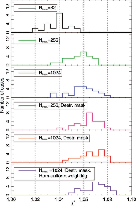
Figure 6 illustrates the effect the approximations inherent in the NCVM computation: horn-uniform weighting; destriping resolution $N_{\rm Destr.}$ equal to the map resolution; and masking in the destriping phase. Each non-ideal factor increases the discrepancy seen in the $\chi^{2}$ test.

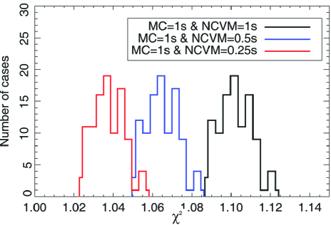
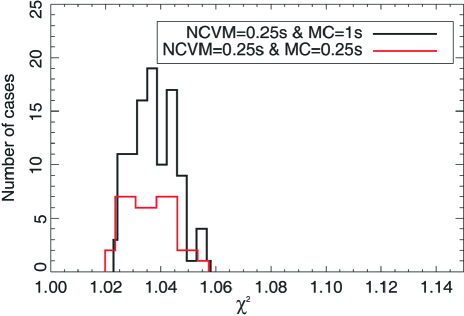
We chose to use shorter baselines in the NCVM production than in the map-making. They were 0.25 s (8 samples), 0.5 s (24 samples), and 0.5 s (39 samples) for 30 GHz, 44 GHz, and 70 GHz, respectively. Since many of the knee frequencies were higher than anticipated prior to launch, short baselines model the noise better (Keskitalo et al. 2010). We additionally found out that reducing baseline length in the NCVM calculation affects the $\chi^{2}$ statistics more than changing baseline length in the mapmaking (see Fig. 7).

Figure 6: Reduced $\chi^{2}$ statistics from 25 noise-only maps for the 30 GHz 2013 delivery. The NCVM was calculated using 0.25 s baselines, while the simulations were made with 0.5 s baselines. The number of idealizations in the noise-only simulations decreases from top to bottom. The first set of simulations (plotted in black) contains the same approximations that are made in the NCVM calculation. The last set of simulations (plotted in purple) corresponds to the standard mapmaking options: the horns are weighted uniformly; destriping resolution, $N_{\rm Destr.}$, is 1024; and a destriping mask is applied.

Figure 7: Reduced $\chi^{2}$ statistics from noise-only maps in the 30 GHz 2013 delivery. Upper: The noise-only simulation set is fixed, while the NCVM baseline length changes. Three baseline lengths were chosen, 1 s (black), 0.5 s (blue), and 0.25 s (red). Lower: the NCVM is fixed, while the noise-only simulation varies. Two baseline lengths were chosen, 1 s (plotted in black) and 0.25 s (red).

9.3 Half-ring noise maps

To estimate the noise directly at the map level and in the angular power spectra, we produce half-ring maps ($h_{1}$ and $h_{2}$) with the same pipeline as described in Sect. 9.1, but using data only from the first or the second half of each stable pointing period. These half-ring maps contain the same sky signal, since they result from the same scanning pattern on the sky. Therefore the difference of maps $h_{1}$ and $h_{2}$ captures any noise whose frequency is greater than that corresponding to half of the duration of the pointing period, i.e., noise whose frequency is $f\gtrsim 1/20\thinspace\mbox{min}=0.85\thinspace$mHz. The procedure of calculating the half-ring maps and their hit-count-weighted difference maps is described in more detail in Zacchei et al. (2011) and Planck Collaboration (2013).

The use of half-ring maps in the validation of data and noise estimates will be explained in Sect. 12. In addition, the half-ring maps were an integral part of the component separation process  (Planck Collaboration XII 2014) and likelihood codes  (Planck Collaboration XV 2014).

9.4 Noise Monte Carlo simulations

Simulated noise timelines are produced according to the three-parameter noise model (white noise sensitivity, knee frequency, slope), using the estimated parameter values given in Tables 9 and  10. Maps are made from these noise timelines using reconstructed flight pointing and the same Madam parameter settings as used for the flight maps. These steps are repeated to produce 1000 realizations of noise maps for different radiometer combinations, including frequency maps and 70 GHz horn-pair maps.

This Monte Carlo (MC) work is done in two stages, with two partially different pipelines, first an LFI MC in close connection with the map-making from the LFI flight data, and then as a part of the joint LFI/HFI full-focal plane “FFP6” simulations. This work is divided between two supercomputing centers, the CSC-IT Center for Science in Finland and the National Energy Research Scientific Computing Center (NERSC) in the U.S.

The noise MC maps provide a statistical distribution of noise maps that can be compared to the half-ring noise maps (Sec. 9.3) to see how well maps from the noise model match the real flight noise in the half-ring noise maps. Note, however, that half-ring noise maps cannot represent properly the noise in the flight maps for timescales of half the pointing period or longer.

For low-resolution studies, the maps are downgraded to $N_{\rm side}=32$ and $N_{\rm side}=16$ HEALPix resolution, using the same procedure as for the flight maps. These can be compared to the low-resolution noise covariance matrices discussed in Sec. 9.2, which were generated from the same noise model, but are based on some approximations (see Fig. 6 and Fig. 7). This comparison reveals the effect of these approximations on the NCVM.

In addition, the noise MC maps were used in power spectrum estimation, component separation (Planck Collaboration XII 2014), and in non-Gaussianity estimation (Planck Collaboration XXIII 2014 and Planck Collaboration XXIII 2014).

9.5 Overview of LFI map properties

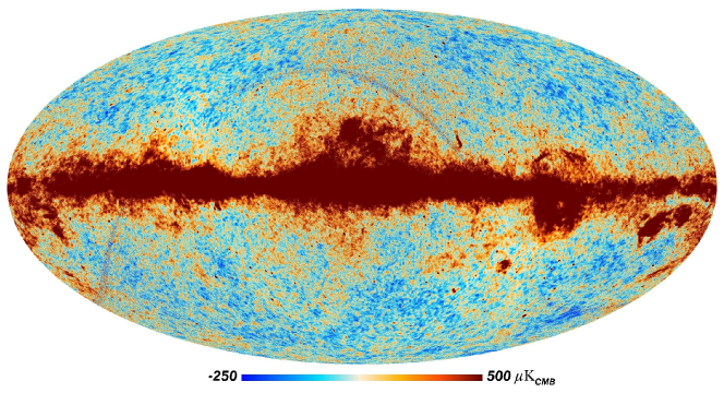
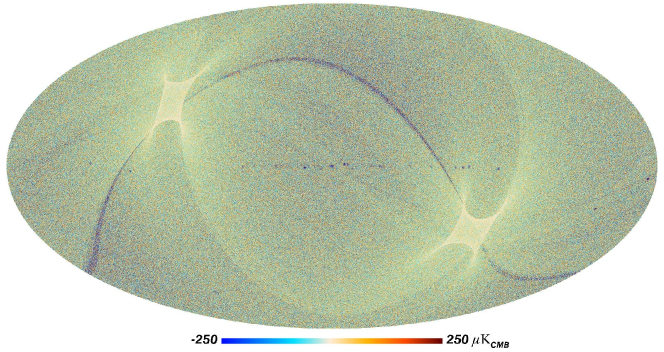
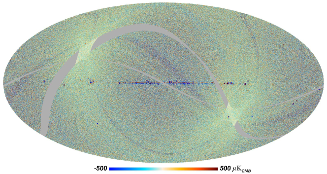
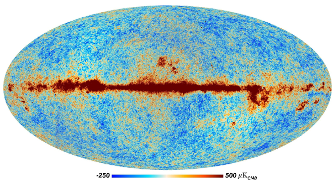
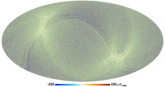
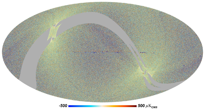
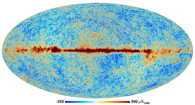
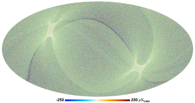
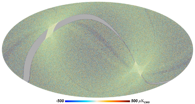
Figures 8 to 10 show the 30, 44, and 70 GHz frequency maps created from LFI data. The top map in each figure is the temperature ($I$) map based on the nominal mission data. The middle row is the difference between maps ($n_{\rm m}$) made of the first and second half of each stable pointing period (half-ring maps) weighted by the hit count calculated from Eq. 20. These maps provide a direct measure of the noise on timescales down to half the pointing period, and are calculated as

Figure 8: LFI maps at 30 GHz.   Top: Intensity $I$.   Middle: Half-ring difference between maps made of the first and the second half of each stable pointing period.   Bottom: Survey1 minus Survey2. Smoothed versions of the half-ring and survey difference maps can be found in Planck Collaboration III (2014).

Figure 9: Same as Fig. 8 for 44 GHz.

Figure 10: Same as Fig. 8 for 70 GHz.

$$n_{\rm m}=\frac{h_{\rm 1}-h_{\rm 2}}{w_{\rm hit}}\thinspace,$$ (19)

where the hit-count weight is

$$w_{\rm hit}=\sqrt{N^{\rm hit}_{\rm full}\left[\frac{1}{N^{\rm hit}_{1}}+\frac{1}{N^{\rm hit}_{2}}\right]}.$$ (20)

Here $N^{\rm hit}_{\rm full}=N^{\rm hit}_{1}+N^{\rm hit}_{2}$ is the hit count of the full map $m$, while $N^{\rm hit}_{1}$ and $N^{\rm hit}_{2}$ are the hit counts of the half-ring maps $h_{1}$ and $h_{2}$, respectively.

The bottom row is the difference between Survey1 and Survey2, and gives information on longer-timescale variations. A dark stripe corresponding to two observing days is visible in the half-ring difference maps and also (faintly) in the frequency maps. This is due to the fact that in the first days of observation the instrument was affected by an occasional bit-flip change in the gain-setting circuit of the data acquisition electronics, probably due to cosmic ray hits. The data acquired before a workaround for the problem was implemented are flagged out, leading to a stripe of reduced integration time and higher noise. One other clear feature can be seen at the Galactic plane in the survey difference maps, especially at 30 GHz. There is an apparent split in intensity (seen as a separation of red and blue) due to the beam ellipticity: the elliptical beam had a different orientation relative to the Galaxy in Survey1 than in Survey2.

10 Polarization

LFI data processing has included analysis of polarization from the beginning, but polarization results are not included in the 2013 data release and scientific analysis because the level of systematic errors in the maps remains above acceptable levels for cosmological work. In this section we outline the polarization-specific steps in the data analysis, quantify the residual systematics, and sketch how we expect to correct them for the next data release.

To an excellent approximation (see Sect. 9.1), the $Q$ and $U$ polarization maps are derived from the difference between the calibrated signals from the two radiometers in each RCA, the main (M) and side arm (S), which are sensitive to orthogonal polarizations. Any differential calibration errors between M and S cause leakage of total intensity into the polarization maps. Such mismatch arises from three main causes:

• differences between the beam profiles of M and S;

• errors in the gain calibration;

• differential color corrections between M and S due to differences in their bandpasses (the “bandpass leakage effect”).

These effects are described in Leahy et al. (2010). Polarization imposes stringent requirements on the accuracy of gain calibration that have driven our choice of calibration scheme (Planck Collaboration V 2014). The control of systematics for polarization also requires precise cancellation of the M and S signals. This underlies our use of identical pointings for the data from the two radiometers in each horn, despite a small amount of beam squint between the polarizations, and also the decision to use horn-uniform weighting. Neither of these choices results in significant degradation to the total intensity maps, although they are slightly sub-optimal from the standpoint of noise.

Bandpass leakage requires a special step in the calibration. The principle instrumental factor controlling bandpass leakage is the effective frequency mismatch between M and S detectors, $a=(\nu_{\mathrm{S}}-\nu_{\mathrm{M}})/2\nu_{0}$, which must be combined with estimates of the “leakage amplitude” of the foreground emission, $L=(\beta_{\mathrm{fg}}-\beta_{\mathrm{CMB}})T_{\mathrm{fg}}$. Because the leakage amplitude relies on products from component separation, maps of $L$ are available at no higher resolution than that of the 30 GHz channel (33.^′16), and are most reliable at lower resolution (1^∘), where our analysis can incorporate the WMAP 22 GHz maps.

In principle, the $a$-factors can be estimated from the bandpass profiles measured in the ground calibration campaign (Zonca et al. 2009), but as anticipated by Leahy et al. (2010), more accurate values can be found from the flight data; a detailed description of our approach to this will be discussed in a future paper. We estimate that our $a$-factors are currently accurate to about 0.05 %, based on the scatter in values derived from multiple calibrators. A bigger problem at present is accurate evaluation of the leakage amplitude, which requires not only excellent separation of CMB and foreground emission, but also accurate estimates of the foreground spectral index within the band. Currently, the combined uncertainty in the bandpass leakage correction is about 0.3 % of the local foreground intensity. This is comparable to the mean polarization fraction along the Galactic plane.

One other parameter must be calibrated for polarization: the precise orientation of the polarization response for each feed horn. This could not be calibrated on the ground; however, as noted by Leahy et al. (2010), knowledge of horn orientation was expected to be better than 1^∘ from construction tolerances alone. In flight, we check these values by observations of the Crab nebula, and the results confirm the orientations to within a few degrees, which is sufficient for analysis of the $E$-mode spectra. At a higher level of precision our estimates of the response orientations are still affected by the uncertainty in $a$-factors, and so as yet we have no evidence to reject the nominal orientation angles.

The most interesting cosmological signal visible in LFI polarization is the large-scale ($\ell<10$) $E$-mode peak due to reionization, at a typical brightness level of 0.3 $\mu$K. Crucial tests of the reliability of this signal are that the $B$-mode and $EB$ cross-correlation spectra should contain negligible signal, since a cosmological $B$-mode signal at this level would correspond to a tensor-to-scalar ratio significantly larger than current upper limits, while the cosmological $EB$ mode is precisely zero in most models. The primary LFI channel for cosmology is 70 GHz, which has the least foreground contamination of all Planck channels. Our likelihood pipeline estimates these spectra using a conservative Galactic mask, and corrects for residual foregrounds based on the Planck 30 GHz map or WMAP maps. With our current calibration, both these spectra contain residuals at a level comparable to the expected $E$-mode signal from reionization. Hence, although the latter is apparently detected, we cannot be confident that the signal is real. This situation is better illustrated in Fig. 11, where we report, at all three LFI frequencies, null-test spectra from survey-survey differences. At all frequencies, the null-test $EE$ spectra are in good agreement with the noise level as determined by half-ring difference maps at multipoles larger of few tens; this is an indication of the data quality at these multipoles. However, residuals are present at very low-$\ell$, especially at 30 GHz and at 70 GHz, and these preclude as yet a proper characterization of the cosmological signal.

Figure 11: Null-test results comparing power spectra from survey difference maps (SS) to those from half-ring difference maps (hr). Some excess at low multipoles is clearly visible at 30 GHz (left), where the main source has been identified as sidelobe pickup. At 44 (center) and 70 GHz (right), there is less low-$\ell$ contribution both in $TT$ and in $EE$, although residuals are still present. For multipoles larger than few tens, null-test $EE$ spectra follow the expected level of noise as traced by half-ring differences.

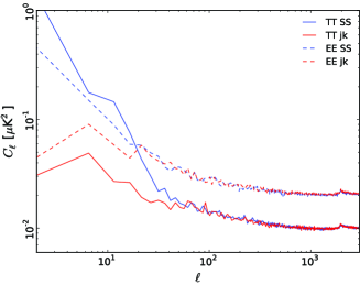
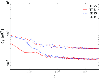
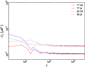
We have simulated the impact of numerous systematic errors to see if they can explain the observed residuals, including foreground correction, bandpass mismatch, Galactic stray light (i.e., leakage through the far sidelobes), and gain errors. None of these simulations has individually generated artefacts as large as those observed. The most likely candidate seems to be in the combination of far sidelobes and calibration errors. As described in Planck Collaboration V (2014), uncertainty in the far-sidelobe pattern is one of the dominant contributors to our calibration uncertainty, as well as making our estimates of the additive effect of Galactic stray light quite uncertain.

11 Power spectra

Temperature power spectra are computed from frequency maps using cROMAster, an implementation of the pseudo-$C_{\ell}$ method described in Hivon et al. (2002). We extend it to derive both auto- and cross-power spectra (see Polenta et al. 2005 for a comparison between the two estimators). Noise bias and covariance matrices are computed through the FFP6 full focal plane simulations, which include 1000 realizations of both signal and noise consistent with Planck data. The angular response of the instrument is accounted for by using the beam window functions presented in Planck Collaboration IV (2014). Coupling kernels to correct for uncompleted sky coverage are computed as described in Appendix D of Planck Collaboration XV (2014). We mask the Galactic plane and unresolved sources using masks described in Sect. 3 of Planck Collaboration XII (2014), in particular, a 70 % Galactic mask for 44 and 70 GHz (70 % of the sky uncovered) and a 60 % Galactic mask for 30 GHz.

Figure 12 shows the 30, 44, and 70 GHz temperature power spectra produced from frequency maps, without diffuse component separation but with a simple correction for unmasked discrete source residuals. There is good agreement between the observed spectra and the Planck likelihood code best-fit model (Planck Collaboration XV 2014).

Figure 12: Temperature power spectra at 30, 44, and 70 GHz. Diffuse foregrounds are reduced only by masking, and a simple foreground component corrects for residual point sources. Dashed lines correspond to the Planck Likelihood Code best fit model.

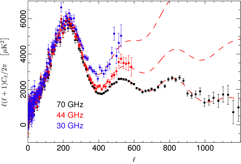
12 Data validation

To assess and verify the quality of the data produced within the data-analysis pipeline, a set of null tests is performed. The main goal is to detect possible instrumental systematic effects. These include effects that are either properly corrected or accounted for later on in the pipeline, effects related to known changes in the operational conditions of the instrument (e.g., the switchover of the sorption cooler), or intrinsic instrument properties coupled to the sky such as stray light from sidelobes. Such tests are also useful for a detailed analysis of the processing steps implemented in the pipeline. Finally, such tests may discover unanticipated problems (e.g., related to different calibration approaches).

Null tests are carried out on blocks of data on different time scales ranging from individual pointing periods to one year of observation, and at different instrument levels (radiometer, horn, and horn-pairs within a given frequency, and at frequency level), for total intensity and, when applicable, for polarization. Such an approach is demanding computationally, and special tools have been built to create a parallel code, compute the null tests, create the output maps and spectra, and build a report from the output from the tests.

The effects probed by null tests depend on the combination of data and time scale treated. For example, differences at horn level between odd and even number surveys clearly reveal the impact of sidelobes, since the sky covered is exactly the same but the orientation of the beam is not. On the other hand, differences between horns for the entire data period may reveal calibration issues or changes in operational or instrumental conditions.

12.1 Null test results

It is important to set pass-fail criteria for such null tests. In general, test failures reveal problems in the data or in the data analysis that must be carefully studied so that specific actions can be taken to mitigate the problems. A simple figure of merit is the actual level of noise in the data derived from half-ring difference maps. Any departure from this noise level would indicate a problem. For example, null-test power spectra are used in Planck Collaboration III (2014) to check the total level of systematic effects in the data. Figure 11 gives results at frequency level of survey-difference null tests for both TT and EE spectra, compared to the noise level derived from half-ring difference maps.

Based on such results we have analyzed our calibration pipeline, particularly the treatment of sidelobes, which has been updated with the inclusion of both the intermediate beam and the in-band beam behavior based on simulations. This will be the final approach for data calibration in the next release.

Although it is clear from these results that a proper treatment of sidelobes is necessary for final refinements in calibration, it is important to note that the overall amplitude of such effects is well below the CMB signal in total intensity, leaving the analysis of the temperature maps totally unaffected.

12.2 Half-ring test

The middle panels of Figs. 8, 9, and 10 show the noise calculated from the hit-count-weighted half-ring difference maps at $N_{\rm side}=1024$, as described by Zacchei et al. (2011) and Planck Collaboration (2013). As a first quality check of the maps, and as one of the tests of the whole data processing pipeline up to the maps, we verify both numerically and visually that the values obtained by dividing the half-ring difference map pixel-by-pixel by the square root of the white noise covariance map (Planck Collaboration (2013)) are approximately Gaussian-distributed with rms near unity. The results are 1.0211, 1.0089, and 1.0007 for 30, 44, and 70 GHz, respectively.

The half-ring difference maps $n_{\rm m}$ are a direct measure of the noise in the actual maps. Models of the noise, required for NCVMs and MC noise realizations, must be validated by comparison to the half-ring difference maps. For this purpose, we calculate the temperature and polarization ($E$- and $B$-mode) auto- and cross-spectra of the half-ring difference maps with anafast, and compare these to the results from the white noise covariance matrices (WNCM) calculated by both Madam and MC noise simulations (Sect. 9.4). Figure 13 gives an example. Further, we calculate the mean $C_{\ell}$ for the high-$\ell$ tails ($1150\leq\ell\leq 1800$) of the noise angular power spectra and take the ratio to the WNCM estimate (Figure 14). As expected, there is some residual $1/f$ noise even in the high-$\ell$ region, i.e., the full noise MCs lead to slightly higher noise predictions than the WNCM or binned white noise from the noise MCs. The residual $1/f$ noise is of the order of 2.5 % at 30 GHz, 1.0 % at 44 GHz, and 0.1 % at 70 GHz. We find good consistency between the noise MCs and the direct noise calculation from the half-ring difference maps: the high-$\ell$ noise from MCs is only 0.8 % higher at 30 GHz, 0.2 % higher at 44 GHz, and 0.1 % lower at 70 GHz than the result from the half-ring differences. The error bars of the noise MC do not include at this stage the uncertainty of noise parameters indicated in Tables 9 and 10. More such comparisons are reported in Planck Collaboration (2013).

Figure 13: Comparison of the noise angular power spectra of half-ring difference maps (red), white noise covariance maps produced by madam (blue), and 101 full-noise MCs for each $C_{\ell}$ (black; for 16%, 50% (bold), and 84% quantiles). In the noise MC case, no errors were propagated from Tables 9 and 10; only the median values of the three noise parameters were used. Those plots validate our capability to model the noise in the TOD in agreement with the half-ring difference maps that give the most direct measure of the noise.

Figure 14: Ratio of the mean noise angular power at high-$\ell$ ($1150\leq\ell\leq 1800$) to the white noise estimate from white noise covariance matrices. The half-ring differences are hit-count-weighted. One hundred and one full noise MC maps were made. The binned white noise is from the noise MC. The “reference” white noise levels (green) are $9.8\times 10^{-15}\thinspace$K², $13.1\times 10^{-15}\thinspace$K², and $10.1\times 10^{-15}\thinspace$K², for 30, 44, and 70 GHz, respectively. In the noise MCs, no errors were propagated from Tables 9 and 10; only the median values of the three noise parameters were used. Therefore the error bars in the noise MCs represent only the statistical variance in the 101 realizations. If the uncertainty of the estimation of the three noise parameters were propagated to the noise MC, the error bars would be much larger.

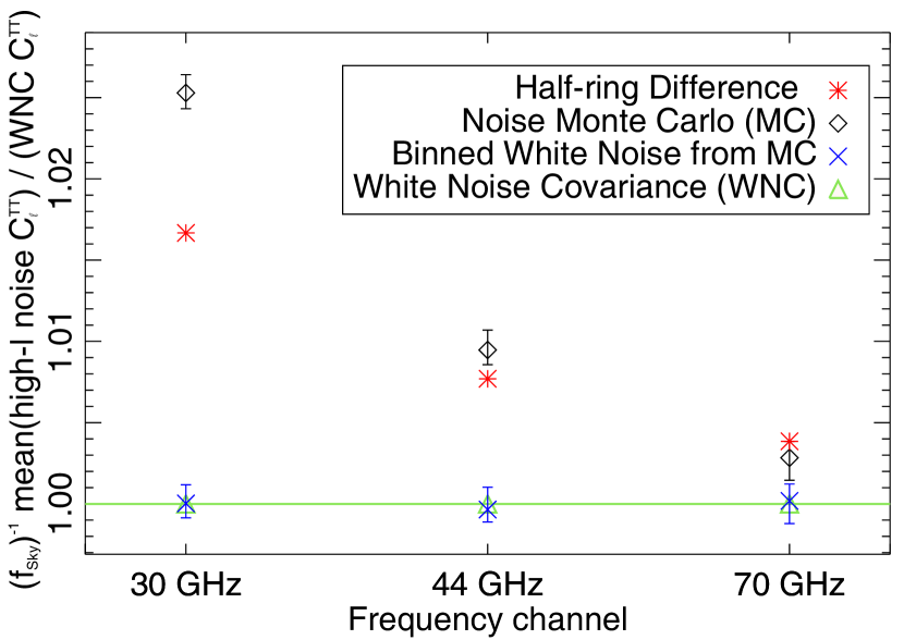
12.3 Intra-frequency consistency check

We have tested the consistency between the 30, 44, and 70 GHz maps by comparing the power spectra in the multipole range around the first acoustic peak. To do so, we remove the estimated contribution from residual, unresolved point sources from the spectra presented in Sec. 11. We then build the scatter plots for the three frequency pairs, i.e., 70 vs. 30 GHz, 70 vs. 44 GHz, and 44 vs. 30 GHz, and perform a linear fit accounting for errors on both axis.

Figure 15: Consistency between estimates of the angular power spectra at frequencies. Left to Right: 70 vs. 44 GHz; 70 vs. 30 GHz; 44 vs. 30 GHz. Solid red lines are the best fit of the linear regressions, whose slopes $\alpha$ are consistent with unity within the errors.

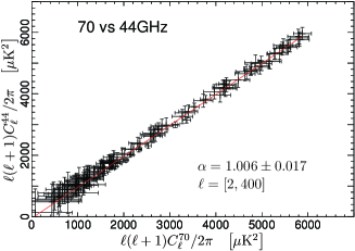
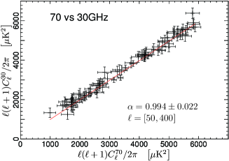
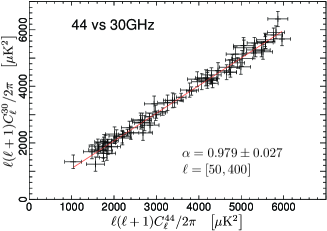
The results in Fig. 15 show that the three power spectra are consistent within the errors. Moreover, the current error budget does not account for foreground removal, calibration, and window function uncertainties. Hence the resulting agreement between spectra at different frequencies can reasonably be considered even more significant. We also compared the flux densities of compact sources at the three LFI frequencies, derived from the PCCS (Planck Collaboration XXVIII 2014), and find these in acceptable agreement.

12.4 70 GHz internal consistency check

We use the Hausman test (Polenta et al. 2005) to assess the consistency of auto- and cross-spectrum estimates at 70 GHz. Define the statistic

$$H_{\ell}=\left(\hat{C_{\ell}}-\tilde{C_{\ell}}\right)/\sqrt{{\rm Var}\left\{\hat{C_{\ell}}-\tilde{C_{\ell}}\right\}}\thinspace,$$ (21)

where $\hat{C_{\ell}}$ and $\tilde{C_{\ell}}$ represent auto- and cross-spectra, respectively. To combine information from different multipoles into a single quantity, we define

$$B_{L}(r)\equiv\frac{1}{\sqrt{L}}\sum_{\ell=2}^{[Lr]}H_{\ell},r\in\left[0,1\right]\thinspace,$$ (22)

where $[.]$ denotes integer part. The distribution of $B_{L}(r)$ converges (in a functional sense) to a Brownian motion process, which can be studied through the statistics $s_{1}=\textrm{sup}_{r}B_{L}(r)$, $s_{2}=\textrm{sup}_{r}|B_{L}(r)|$, and $s_{3}=\int_{0}^{1}B_{L}^{2}(r)dr$. Using the FFP6 simulations, we derive the empirical distribution for all three test statistics, and then compare them with the results obtained from the Planck data themselves (see Fig. 16). The Hausman test shows no statistically significant inconsistencies between the two spectral estimates.

Figure 16: Empirical distributions estimated via FFP6 of the $s_{1}$ (left), $s_{2}$ (middle), and $s_{3}$ (right) statistics (see text). The vertical line represents 70 GHz data.

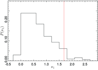
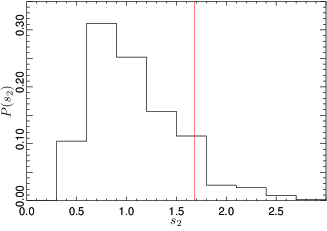
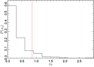
As a further test, we estimate the temperature power spectrum for each of the three horn-pair maps, and compare the results with the spectrum obtained from all 12 radiometers shown above. Figure 17 shows the difference between the horn-pair and the combined spectra. Again, the error bars have been estimated from the FFP6 simulations. A $\chi^{2}$ analysis of the residual shows that they are compatible with the null hypothesis, confirming the strong consistency of the estimates.

Figure 17: Residuals between the auto-spectra of the horn pair maps and the power spectrum of the full 70 GHz frequency map. Error bars are derived from the FFP6 simulations.

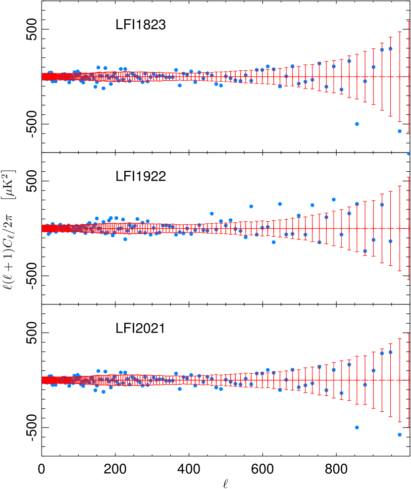
12.5 Updated systematic effects assessment

Known systematic effects in LFI are reported in detail in  Planck Collaboration III (2014) and summarized in Table 12, which lists both the rms and the difference between the 99 % and the 1 % quantiles in the pixel value distributions. We refer to it as the peak-to-peak (p-p) difference even though it neglects outliers, as it effectively approximates the peak-to-peak variation of the effect on the map.

Table 12: Effect of known systematic uncertainties on maps^a

Effect in maps [$$\mu$$K_cmb] 30 GHz 44 GHz 70 GHz Systematic p-p rms p-p rms p-p rms Bias fluctuations. 0.08 0.01 0.10 0.02 0.23 0.06 Thermal fluctuations. 0.61 0.11 0.40 0.08 1.17 0.20 1-Hz spikes. 0.87 0.17 0.14 0.03 0.60 0.12 Sidelobe pickup. 18.95 4.53 1.92 0.57 6.39 1.91 ADC non-linearity. 3.87 1.01 0.89 0.19 0.92 0.19 Gain residuals. 4.33 1.16 4.74 0.97 6.51 1.10 Total. 21.02 4.83 5.61 1.13 7.87 2.00

^aCalculated on a pixel of size equal to the average beam FWHM.

Our analysis  (Planck Collaboration III 2014) shows that systematic uncertainties are at least two orders of magnitude below the CMB temperature anisotropy power spectrum, and are dominated by stray light pick-up from far sidelobes and imperfect photometric calibration.

13 Infrastructure overview

The computer cluster used for the maps productions has ten 64-bit nodes with two single-core CPUs and 16 GB of RAM, and ten 64-bit nodes with two motherboards, each with two six-core CPUs and 72 GB of RAM. The total RAM available exceeds 1.5 TB, sufficient to allow for the creation of all maps until the end of the mission. The dual-motherboard nodes are connected through an InfiniBand 40 Gbit network interface, while a 1 Gbit interface is provided for the other connections.

The hardware infrastructure includes a front-end machine (two quad-core CPUs, 8 GB of RAM), which is the access point for users and hosts the pbs server, and a control machine running the LDAP authentication server and the DNS and DHCP services.

The software used for system management and synchronization includes kickstart and puppet, while parallelization of the computations is guaranteed by the torque resource manager and the maui scheduler.

Data products are stored and organized into three different servers that host the Level 1, Level 2, and test databases (Fig. 1). For each database, there is associated RAID 6 storage, with up to 40 TB formatted with the JFS filesystem.

14 Discussion and conclusions

We have described the pipeline used to process the first 15.5 months of Planck/LFI data from Level 1 through temperature frequency maps, and the assessment of the quality of the products, which is largely based on null tests. Companion papers provide full descriptions of three critical aspects of the data analysis and products delivered: Planck Collaboration III (2014) analyzes systematic effects and assesses their impact; Planck Collaboration V (2014) describes photometric calibration; and Planck Collaboration IV (2014) describes beam patterns and window functions. The Planck Explanatory Supplement (Planck Collaboration 2013) provides a detailed description of all the products delivered in this release.

The Level 1 pipeline has not changed since the start of the mission in 2009, and has been running flawlessly and continuously, demonstrating the robustness of the design and development approach. In contrast, the Level 2 pipeline has been largely restructured (see Zacchei et al. 2011 for a description of the initial pipeline). The major improvements involved new procedures for pointing reconstruction, detailed estimation of systematic effects, and photometric calibration. These improvements allow us to obtain, as reported in Table 1, a final calibration uncertainty of the order of 0.6%, and also to propagate, using simulations, known systematic effects into the final product maps. The impact of the combination of all known systematic effects is at least two orders of magnitude below the CMB temperature anisotropy power spectrum.

Particular emphasis is given to null tests, which are routinely applied to various subsets of the data in order to assess the scientific quality of the LFI products. The null test procedure, described in Sec. 12, allowed us to detect and solve a number of problems in the Level 2 pipeline that emerged during the processing period. In fact, the pipeline is still being optimized and more improvements are planned for the next data release. Future improvements will be aimed at obtaining high-quality polarization results, which require control of spurious effects at sub-microkelvin level, as well as better characterization of the beams, taking into account second order effects such as the bandpass response of each diode and Galactic stray light (i.e., leakage through the far sidelobes).