On the Behavior of RObust Header Compression U-mode in Channels with Memory

Abstract

The existing studies of RObust Header Compression (ROHC) have provided some understanding for memoryless channel, but the behavior of ROHC for correlated wireless channels is not well investigated in spite of its practical importance. In this paper, the dependence of ROHC against its design parameters for the Gilbert Elliot channel is studied by means of three analytical models. A first more elaborated approach accurately predicts the behavior of the protocol for the single RTP flow profile, while a simpler, analytically tractable model yields clear and insightful mathematical relationships that explain the qualitative trends of ROHC. The results are validated against a real world implementation of this protocol. Moreover, a third model studies also the less conventional yet practically relevant setting of multiple RTP flows.

I Introduction

The concept of header compression has been applied very successfully in the wired world and has lead to very effective compression of long IP headers. Since the headers of two consecutive IP packets are highly correlated, the essential idea is to transmit the compressed version of the difference between these headers. This compression can be very effective, but is also fragile to packet losses. While such losses do not frequently happen over wires, they are far more common for the wireless medium. Hence, the traditional header compression mechanism is inadequate to withstand these error ratios and ROHC has been introduced [1, 2, 3, 4].

The ROHC protocol has been developed and standardized by the IETF in 2001 and aims at reducing the header sizes of IP packets to be sent through a cellular link. It offers a strong resilience against channel losses and yet a high compression efficiency. The scheme is so effective that it has found its way in important wireless standards like HSPA and LTE [4, 5, 6], and is being currently proposed for the next generations of DVB RCS and DVB SH. The majority of the past studies are simulation-based, and investigate the performance of ROHC in different environments [2, 6, 7, 8, 9, 10, 11]. On the other hand, only a limited amount of research has tried to analytically describe ROHC [12, 13, 14, 15]. These models can be quite accurate but they do not provide simple expressions and hence rarely do they offer deep insight in the behavior of the protocol as a function of important design parameters or of the channel characteristics. Moreover, all models (except for [13]) are derived for memoryless channels and for traffic with just a single RTP/UDP/IP flow, while in fact the wireless medium is often correlated in time and ROHC leads to interesting capacity improvements especially if several flows are multiplexed together [10].

Our investigation has focused on the performance of ROHC in correlated channels, in particular the Gilbert-Elliott one [16]. The core contribution of our work lies in the development of three analytical models for ROHC. The first one accurately mimics the effective behavior and performance of single-RTP-flow ROHC with the Gilbert-Elliott channel. The second model is a simplified version of the first one that still fairly predicts the trends of ROHC but can be solved in closed form and yields simple and insightful formulae. These results enable to draw useful relationships between the system performance and the design parameters, like the timeout for the transmission of the uncompressed headers or the interpretation window. The third model explores the effect of multiplexing several RTP/UDP/IP flows together on the system performance. Our contribution serves two main purposes: on the one hand, to better characterize the performance of ROHC in correlated channels, on the other hand to provide simple and useful relationships for the design and tuning of a ROHC system.

The rest of the paper is organised as follows. Section II introduces the system model and recalls the most relevant properties of ROHC for the present discussion. Section III describes the three proposed analytical models, which represent our main contribution. The trends and predictions are numerically studied in Section IV, while Section V draws the conclusions.

II System Model

A slotted system with a single transmitter is considered. Without loss of generality, a setting with only one receiver is studied. The transmitter (or source, in the rest of this paper) can either generate one single packet stream for which a ROHC profile between 1 and 4 applies or multiplexes $M$ different RTP/UDP/IPv4 flows. In the former case, the applicable protocols are RTP, UDP, ESP and IP. It is assumed that the source is saturated and has an available packet for transmission in every slot.

The channel is regarded as a Gilbert Elliott packet deletion channel [16]. This channel is modeled by means of a two-state Markov chain: the good state G (correct reception of the packet) and the bad state B (the packet is lost and the upper layers are not aware that a packet was sent). Let us define as $\mathcal{P}$ the one step transition matrix of the Markov chain and as $P_{\text{X,Y}}$ the transition probability from state $X$ to $Y$, $X,Y\in\{\text{G},\text{B}\}$. The transition matrix is uniquely determined by $P_{\text{G,B}}$ and $P_{\text{B,G}}$, which are inversely proportional to the average time spent in the good and bad state, $L_{\text{G}}$ and $L_{\text{B}}$, respectively. The Gilbert-Elliott channel is also equivalently defined by the average duration of a sequence of consecutive bad states $L_{\text{B}}=1/P_{\text{B,G}}$ and the average deletion probability $\epsilon=P_{\text{G,B}}/(P_{\text{G,B}}+P_{\text{B,G}})$ [16]. We remark the assumption of packet deletion, rather than erasure [17]. It turns out that ROHC does not assume that the lower layers would provide a feedback to the IP and above layers in case the packet was not successfully decoded. Hence, the packet is either correctly received or the ROHC receiver is simply unaware of the loss and therefore the terms "packet loss" and "packet deletion" will be used interchangeably in the rest of this paper. Finally we also remark that this channel model holds for consecutively transmitted packets, by other words it is satisfactory for the single RTP flow setting ($M=1$). The necessary modifications for $M>1$ will be explored in Section III-C.

In the rest of this section, a quick introduction on ROHC and on the investigated elements shall be provided. Three different modes of operation can be used in ROHC: Unidirectional (U), Bidirectional Optimistic (O) and Bidirectional Reliable (R). The major difference between these three modes is how the state transitions are handled and the lack of a feedback channel for the U-mode. Moreover every protocol (IP, UDP, RTP) is linked to a specific configuration of ROHC called profile [1]. The focus within this paper is on the U-mode and on the RTP/UDP/IP, UDP/IP, ESP/IP and IP profiles (i.e., profiles 1 to 4, respectively). We refer to [1] for a detailed description of the O-mode and R-mode.

ROHC has two main key properties, namely its efficiency and its robustness. ROHC achieves a very high compression efficiency thanks to properly tuned state machines at the compressor and decompressor sides, which are based on the fact that the fields of a packet header are classified into two categories: static (such as UDP Port numbers) and dynamic (such as the Hop Limit in IPv6 or the Identification in IPv4). The compressor sends first uncompressed packets called Initialization and Refresh (IR) packets, so that both the compressor and the decompressor can initialize their context by storing information concerning the header. Once the compressor is confident enough that the decompressor successfully received an IR packet (by use of ACK for O- and R-mode or by sending $L$ IR packets for the U-mode), it switches forward to an intermediate compression state (First Order (FO), where only the dynamic fields of the header are sent uncompressed) or directly to a full compression state (Second Order (SO), where the header is entirely compressed) as displayed in Fig. 1. In U-mode two different timeouts are used to periodically switch downward to less efficient compression states (IR and FO Timeouts). These two timeouts ensure the context synchronization between the compressor and decompressor since no feedback channel is considered in U-mode. Finally transitions from IR to more compressive states work based on the optimistic approach as shown in Fig. 1 and explained in [1].

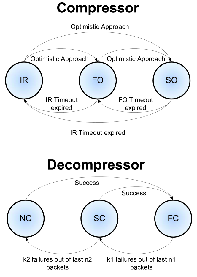
Figure 1: ROHC state machines of the compressor and decompressor in U-mode.

The state machine at the decompressor side is also composed of three states. After the initialization of the context due to the good reception of an IR packet, the decompressor moves from the No Context (NC) state where only IR packets can be decoded to the Full Context (FC) state where all kinds of ROHC packets (IR, FO, SO) can be decompressed (Fig. 1). The decompressor switches from FC to SC only if $k_{1}$ packets out of the last $n_{1}$ received packets have been unsuccessfully decoded (CRC failed).l In this intermediate state (Static Context (SC)) the decompressor can only decode IR or FO packets. Therefore if it receives one of them and the decompression is successful, it moves back to the FC state. However, if over the last $n_{2}$ received packets, $k_{2}$ had a CRC failure, the decompressor moves downward to the NC state, where it will wait for an IR packet (all other received packets in this state are dropped). We refer to [1, 18, 4, 14] for further information.

The second key property of ROHC is its ability to resist to larger packet error ratios than classic header compression schemes. This very high robustness is achieved by the combined use of an encoding scheme and of a second algorithm which is employed when too many consecutive packets are lost [18]. The starting point is the fact that a SO packet of profiles 1 to 4 includes a compressed version of a suitable sequence number (e.g., the RTP SN in profile 1 or the UDP SN generated by ROHC in profile 2). The encoding scheme called Window-based Least Significant Bits (W-LSB) is defined by an interpretation interval $[-p,2^{k}-1-p]$ of size $2^{k}$, where $k$ represents the $k$ least significant bits of the encoded field value and $p$ the offset with respect to the previously received field value [1, 13]. If the SN of the received packet belongs to the interpretation interval, the header can be successfully decompressed and the context updated. Therefore, up to $2^{k}-1-p-1$ packets can be lost in a row without losing synchronization between compressor and decompressor, since field values undergoing small negative changes are not considered here. The second algorithm is called LSB wraparound and enhances the robustness of ROHC by shifting the interpretation interval of $2^{k}$ when more than $2^{k}-1-p-1$ consecutive packets are lost [1]. Thus, the maximal number of packets that can be deleted in a row while still retaining context synchronization can be defined as [18]:

$$\vspace{-5pt}W=(2^{k}-1-p)-1+2^{k}=2^{k+1}-2-p$$ (1)

If more than $W$ packets are lost in a row, the decompressor is not able to decode the next arriving SO packet and is said to be out-of-synchronization. When the receiver is out-of-synchronization and in FC or SC state, the reception of an IR or FO packet enables to retrieve the synchronization, whereas in the NC state the decompressor only updates its context by means of an IR packet.

If several RTP/UDP/IPv4 flows are multiplexed through the same compressor, the IP identifier is increased by one for each outgoing packet from the source [1]. Focusing on one of these RTP flows, the IP identifier will not increase linearly since packets from other RTP flows may be inserted between two packets from the tagged flow. Fig. 2 shows an example where the focus is on the first flow. Hence, the IP identifier can not be retrieved from the SN and must be sent in the compressed header [1]. According to [1], the same W-LSB encoding scheme is used to encode the IP identifier field, although with different values of $k$ and $p$ with respect to the ones used to encode the SN. Thus, the interpretation interval is equal to $[-p,2^{k_{o}}-1-p_{o}]$. In addition, since no wraparound algorithm is used [1], $W_{o}$ can be defined as the upper limit of this interpretation interval:

$$\vspace{-5pt}W_{o}=(2^{k_{o}}-1-p_{o})-1$$ (2)

This means that if the IP identifier increases by more than $W_{o}$ between two consecutively correctly received packets of the same RTP flow, the decompressor will not be able to decode the next packets since too many IP packets from other RTP flows have been inserted.

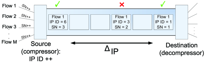
Figure 2: $M$ different RTP flows multiplexed using the same compressor and decompressor

Thus for a single flow communication ($M=1$) $W$ is the only key parameter for the definition of the ROHC robustness, whereas in the case of multiple RTP sources the robustness of the header compression scheme is limited by:

• $W$, which gives the maximum number of packets from the same RTP flow that can be lost in a row and still keeping the context synchronization;

• $W_{o}$, which specifies the maximum number of IP packets that can be inserted between two consecutive packets from the tagged RTP flow without losing the synchronization between the compressor and the decompressor.

III Model Derivation

Out of the description of the ROHC protocol provided in Section II, an important observation can be made, which is at the basis of the first two models.

It happens in many circumstances that all fields of the header to be compressed can be inferred from just one field. For instance, this can be the case in Profile 1 for RTP/UDP/IP headers, when all dynamic fields have a constant known offset with respect to the RTP Sequence Number, whereas the static ones are already stored in the context [1].l In such cases, the Window LSB encoding method guarantees that the key field can be correctly retrieved as long as no more than $W$ headers are deleted in a row. Our model works for any ROHC profile for which the previous property holds. For example, profiles 1 to 4, where the sender side needs to compress only one header field (excluding the CRC) and the decompressor can retrieve all other fields from the compressed one. In these cases, if a single flow is present, the only field to encode is the RTP, UDP, ESP or IP Sequence Number (SN), respectively.l The SN is incremented by one for each sent packet and is to be used by the receiver to detect packet losses and to reorder the packets.

In some other cases, more than one dynamic field can often change its value and hence two or more fields need to be compressed. Model 3 will explore one such examples for the specific case of RTP/UDP/IPv4 headers, when multiple RTP flows are multiplexed in the same IP flow. In this setting, the IP ID field ceases to have a constant known offset from the RTP SN and the compressor can resort, for instance, to offset encoding or scaled encoding [1], Sections 4.5.3 and 4.5.5, respectively.

III-A Model 1: Single Flow, full representation

On the basis of these observations, a realistic Markov chain fully compliant with the ROHC standard has been derived (model 1). The states of this Markov chain can be arranged in a two dimensional array which tracks on the one dimension the number of packets lost in a row and on the other dimension the kind of ROHC packets transmitted by the compressor. Fig. 3 depicts a simplified scheme of this Markov chain where the states for which the compressor and the decompressor share the same state are coalesced in ellipses. For a better understanding the status of the state machines of the compressor and the decompressor have been added.

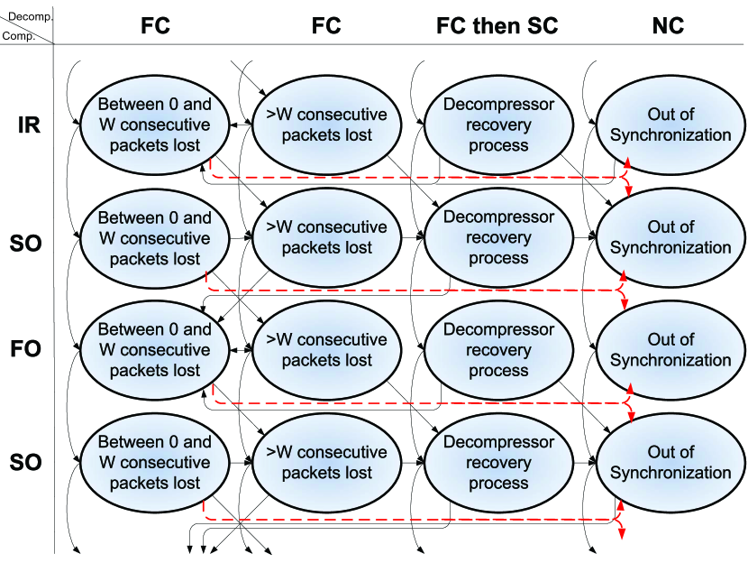
Figure 3: Simplified Markov chain model for the ROHC modeling in U-mode - model 1

Each of the ellipses displayed in Fig. 3 may contain more than one state (up to a few hundred for some ellipses). This detailed model turns out to be accurate, but is not amenable to mathematical analysis due to its large size since it can reach thousands of states depending on the configuration of the ROHC parameters. Each row of the array in Fig. 3 describes the kind of ROHC packets that have been sent by the compressor. As explained in Section II, when the decompressor is in FC or SC state and more than $W$ packets have been lost consecutively, the synchronization is retrieved upon a correct acquisition of an IR or FO packet whereas only the correct reception of an IR packet enables the decompressor to recover the synchronization when it is in NC state. Thus the type of sent packets is a parameter to be compulsory tracked.

The second parameter to be followed is the number of consecutively lost packets (tracked by the columns of the matrix). Here the major point to differentiate is whether more than $W$ packets have been deleted consecutively or not (represented by the two first ellipses of each line in Fig. 3). In order to correctly model the ROHC standard, an additional ellipse has been represented before the out-of-synchronization state so as to map the behavior of the decompressor upon the correct reception of a ROHC packet when more than $W$ packets have been lost consecutively (third ellipse of each line). According to [1] the synchronization can be retrieved if a FO or IR packet is correctly received although more than $W$ packets have been deleted in a row. This is due to the "$k$ out of $n$" rule used by the decompressor to recover a packet [1, 18]. This rule explains the two possible states of the decompressor for this ellipse as well ("FC then SC"). Finally the last ellipse of each line in Fig. 3 represents the out-of-synchronization state when the decompressor can not decode any packet and is waiting for the correct reception of an IR packet to retrieve the synchronization. Since a Gilbert-Elliott deletion channel is considered, this ellipse contains in reality two out-of-synchronization states: one for the good state and one for the bad state.

A full description of the model cannot be provided due to reasons of space. However, the ellipse from the second row, first column of Fig. 3 will be further explained, as the inner structure of the other regions of the Markov chain is similar. This ellipse is composed by $W+1$ columns (each tracking a different value of $w$) and as many rows as the time between the expiration of the IR timeout and the transmission of the next FO header. Let us assume to be in a generic state of this ellipse. Every time a new header is sent, the chain transitions to the next row below. If the column is the first one, the channel must have been in the non-deletion state ($G$), otherwise it is in the deletion ($B$) state. The decompressor correctly receives the next header if the channel will not be in the bad state, which happens with probability $P_{\text{G,G}}$ and $P_{\text{B,G}}$, respectively, and will transition into the first column. Otherwise, the column index will increase by one. If $w$ was already $W$, the chain transition into the next ellipse to the right.

Moreover in order to be fully compliant with the ROHC protocol, the errors due to a wrong CRC check in the robustness mechanism have been introduced (represented by the dashed red arrows in Fig. 3). To better understand this issue let us write $W$ as follows:

$$\vspace{-5pt}W=W_{1}+W_{2}$$ (3)

where

$$W_{1} = (2^{k}-1-p)-1$$ (4)

$$W_{2} = 2^{k}$$ (5)

As explained in Section II, if more than $W_{1}$ but less than $W_{2}$ packets are lost in a row, ROHC applies the wraparound algorithm to enhance its robustness. However, before applying this algorithm, ROHC tries a first time to decode the received packet and performs a CRC check. Since more than $W_{1}$ packets have been lost consecutively, ROHC can not retrieve the received packet without the wraparound algorithm and the CRC check is therefore wrong. As the decompressed packet did not pass the CRC check, ROHC applies the wraparound algorithm and tries to decode the packet again, but this time the interpretation interval is shifted and hence a new header is reconstructed. If the new CRC check is successful the packet will be forwarded to the higher layers. As explained in the Appendix, the CRC at the first attempt may nonetheless yield a false negative with a probability of 1/32 (i.e., the packet is wrong but the CRC check did not realize it). In this case, the wrong packet is regarded as valid and is forwarded to the upper layers which will not be able to interpret it. This wrong interpretation of the CRC explains why the chain can switch directly from the first ellipse of each line to the out-of-synchronization state.

The probability of losing synchronization between the compressor and decompressor can be numerically computed as the sum of the steady state probabilities of being in one "OoS" state (see the last column of Fig. 3). This out-of-synchronization (OoS) probability only depends on the ROHC design parameters (L, IRT) as well as on the characteristics of the wireless channel. The accuracy of this model makes it suitable to provide a quick yet faithful evaluation of the protocol performance. However, this model offers neither a simple relationships between the above mentioned metrics nor deep insight into the protocol behavior.

III-B Model 2: Single Flow, simplified representation

The model that has been described in the previous subsection faithfully represents the behavior of the ROHC protocol and Section IV will prove the very good match between predictions and real world measurements. The previous model is however quite elaborated and does not enable to derive simple relationships of the system performance. The goal of the second part is to devise a model with far fewer states, that yields clear closed form expressions for the OoS probability and hence more insight on the behavior of ROHC, yet at no major loss of modelling accuracy.

In order to characterize the system, three elements must be modelled: the compressor, the channel, and the decompressor. The model described within this subsection (model 2) is based on a set of assumptions, which aim to reduce the complexity of model 1 while still correctly predicting the qualitative trends of the protocol performance against the design parameters. These assumptions are listed hereafter:

• Channel model: A Gilbert-Elliott packet deletion channel is considered, as stated in Section II.

• Compressor: The FO packets are not taken into account for this model because of their limited actual impact. Moreover, $L=1$ for the sake of simplicity, while $L$ is arbitrary in model 1. The compressor state machine comprises only two states: IR and SO states. Moreover, it is assumed that the compressor decides the type of the packet between IR and SO independently in every slot. An IR frame is generated with probability $P_{\text{IR}}$, and therefore the number of SO frames between two IR packets (i.e., the IR timeout) follows a memoryless, geometric random variable with average value:

  $$\vspace{-5pt}\text{IRT}=\frac{1}{P_{\text{IR}}}$$ (6)

  By means of these assumptions, the IRT is no longer deterministic and becomes geometric. Thus the knowledge of the compression level of the previous packets is not required anymore. We remark that some models of other systems which employ backoffs to resolve collisions also assumed a geometric backoff to yield more tractable formulae, even though such quantity can have other distributions in practical realisations of these systems (see for instance the analysis of IEEE 802.11 [19] or of ALOHA [20]). The qualitative trends of the system are still correctly predicted, while the numerical performance is often about the same up to a multiplicative constant. Section IV provides a validation of this claim against a real world measurement.

• Decompressor: Since no FO packets are considered, the SC state of the decompressor is omitted as well. Therefore the decompressor state machine is composed of two states (the NC and the FC states). The key element to track is the number of consecutively lost packets. The following modelling assumptions for the decompressor have been included:

  • If no packets are lost, the decompressor remains in FC state and works properly.

  • If no more than $W$ packets are lost in a row due to channel impairments, the decompressor is still able to decode the next SO packets thanks to the ROHC algorithm.

  • However if the decompressor realises that more than $W$ packets are lost, there is a major context damage and the decompressor cannot interpret the next arriving packet. Thus it switches back directly to the NC state and waits for an IR packet. Neither the $k_{1}$ out of $n_{1}$ nor the $k_{2}$ out of $n_{2}$ rules are considered. Until the correct reception of an IR packet, the decompressor is out-of-synchronization.

The decompressor loses synchronization if more than $W$ packets in a row have been lost and after this event one SO packet is received. We remark that the last condition is important: if the decompressor never received packets, it would not be aware of the synchronization loss.

While the decompressor is synchronized, the model tracks the number $w$ of consecutively lost packets. Thus the model developed here is a Markov chain in which $W+1$ states track the value of $w$, $0\leq w\leq W$. If more than $W$ packets have been corrupted by the channel, the decompressor may not yet be aware of the loss of synchronization and the chain remains in a state "$W^{+}$" until a packet is correctly delivered by the physical layer (note that in this situation the channel must have transitioned from the bad to the good state). If the packet is an IR frame, the node retrieves synchronization and returns to the $w=0$ state. Otherwise, the decompressor realises it has lost synchronization and moves into a (OoS, G) state, where the G represents the channel condition. The chain remains in the (OoS, G) until either the channel transitions into the B state (and hence the chain moves into (OoS, B)) or an IR packet is received, and thus the decompressor recovers the synchronization and can return to the $w=0$ state. The decompressor has lost synchronization when it is in either the (OoS, G) or (OoS, B) state.

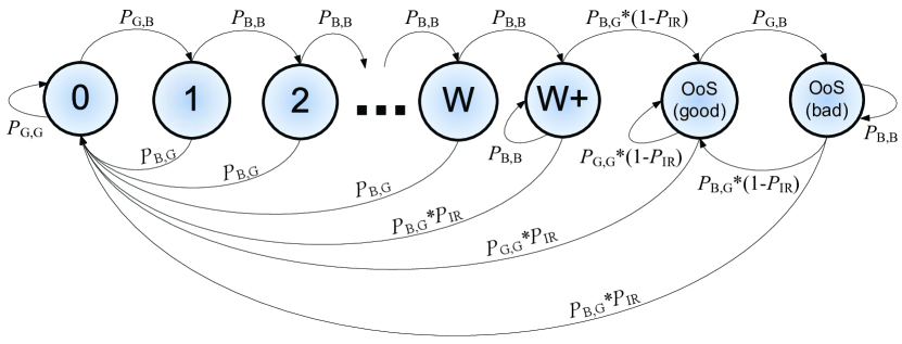
Figure 4: Markov chain model for the ROHC modeling in U-mode - model 2

Fig. 4 depicts this Markov chain model and its transition probabilities. Let us denote by $\pi_{w},\,\pi_{W^{+}},\,\pi_{\text{OoS,G}},\,\pi_{\text{OoS,B}}$ the steady state probabilities of state $w$, $W^{+}$ and of the two out-of-synchronization states, respectively. The solution of the chain is in principle straightforward, although tedious. Some steps will be nonetheless provided. The key goal is to compute the probability $\pi_{0}$ of the $w=0$ state, as all other steady state probabilities can be written as a function of $\pi_{0}$. These probabilities turn out to be equal to:

$$\pi_{w} = P_{\text{G,B}}(P_{\text{B,B}})^{w-1}\pi_{0},\,0\leq w\leq W$$ (7)

$$\pi_{W^{+}} = \frac{P_{\text{G,B}}(P_{\text{B,B}})^{W}}{P_{\text{B,G}}}\pi_{0}$$ (8)

$$\pi_{OoS,G} = \frac{P_{\text{G,B}}(P_{\text{B,B}})^{W}(1-P_{\text{IR}})}{P_{\text{IR}}}\pi_{0}$$ (9)

$$\pi_{OoS,B} = \frac{P_{\text{G,B}}(P_{\text{B,B}})^{W}(1-P_{\text{IR}})}{P_{\text{IR}}}\frac{P_{\text{G,B}}}{P_{\text{B,G}}}\pi_{0}$$ (10)

Through these equations, the steady state solution can be computed by means of the normalization condition (Eq. (11)):

$$1 = \sum_{w=0}^{W}\pi_{w}+\pi_{W^{+}}+\pi_{OoS,G}+\pi_{OoS,B}$$ (11)

$$\pi_{0} = \frac{1}{1+F_{W}+F_{\text{OoS}}}$$ (12)

$$F_{W} = \frac{\sum_{w=1}^{W}\pi_{w}+\pi_{W^{+}}}{\pi_{0}}=\frac{P_{\text{G,B}}}{P_{\text{B,G}}}$$ (13)

$$F_{\text{OoS}} = \frac{\pi_{\text{OoS,G}}+\pi_{\text{OoS,B}}}{\pi_{0}}=$$ (14)

$$= \frac{P_{\text{G,B}}}{P_{\text{B,G}}}(P_{\text{B,B}})^{W}(P_{\text{B,G}}+P_{\text{G,B}})\frac{1-P_{\text{IR}}}{P_{\text{IR}}}$$

We shall define the probability of being out of synchronization as $P_{\text{OoS}}$, which is equal to the probability of being in either state (OoS,G) or (OoS,B):

$$P_{\text{OoS}} = \pi_{\text{OoS,G}}+\pi_{\text{OoS,B}}=$$ (15)

$$= \frac{\frac{P_{\text{G,B}}}{P_{\text{B,G}}}(P_{\text{B,B}})^{W}(P_{\text{B,G}}+P_{\text{G,B}})\frac{1-P_{\text{IR}}}{P_{\text{IR}}}}{1+\frac{P_{\text{G,B}}}{P_{\text{B,G}}}\left(1+(P_{\text{B,B}})^{W}(P_{\text{B,G}}+P_{\text{G,B}})\frac{1-P_{\text{IR}}}{P_{\text{IR}}}\right)}$$

Eq. (15) is not particularly insightful but can be simplified under reasonable hypotheses in realistic settings. First of all, it shall be assumed that $\epsilon\ll 1\rightarrow L_{\text{B}}\ll L_{\text{G}}\rightarrow P_{\text{G,B}}\ll P_{\text{B,G}}$. This means that the channel does not introduce too many errors (say, below 10%). Hence, the denominator of Eq. (15) is very close to (just slightly larger than) 1. Moreover, the IR timeout will be assumed to be much larger than 1 (otherwise, uncompressed packets are sent too often and the ROHC efficiency is too low), thus $P_{\text{IR}}\simeq 0$. The numerator can be approximated as:

$$P_{\text{OoS}} \simeq \frac{P_{\text{G,B}}}{P_{\text{IR}}}(1-P_{\text{B,G}})^{W}=\frac{1}{L_{\text{G}}}\left(\frac{L_{\text{B}}-1}{L_{\text{B}}}\right)^{W}\text{IRT}\simeq$$ (16)

$$\simeq \frac{\epsilon}{L_{\text{B}}}\left(1-\frac{1}{L_{\text{B}}}\right)^{W}\text{IRT}$$

The expression links the two parameters that describe the Gilbert-Elliott channel ($\epsilon$ and $L_{\text{B}}$) and the two ROHC design parameters $W$ and IRT with the OoS probability, which is our main metric.

A natural question is how to pick the value of $W$ so that $P_{\text{OoS}}\ll\epsilon$, that is to say, how to design the system so that the OoS probability does not significantly worsen the intrinsic error ratio of the channel. Let us define as $A$ the ratio $P_{\text{OoS}}/\epsilon$ and let us set $A\gtrsim 0$ (in practice, $A<0.1$). Hence:

$$\vspace{-5pt}W=\frac{\log\left(\frac{AL_{\text{B}}}{\text{IRT}}\right)}{\log\left(1-\frac{1}{L_{\text{B}}}\right)}$$ (17)

If in addition $L_{\text{B}}\gg 1$, $\log(1-1/L_{\text{B}})\simeq-1/L_{\text{B}}$ and thus:

$$\vspace{-5pt}W\gtrsim\frac{\log\left(\frac{AL_{\text{B}}}{\text{IRT}}\right)}{-\frac{1}{L_{\text{B}}}}=-L_{B}\log\left(\frac{AL_{\text{B}}}{\text{IRT}}\right)=L_{B}\log\left(\frac{\text{IRT}}{AL_{\text{B}}}\right)$$ (18)

This equation formally proves an intuitive fact: in the Gilbert-Elliott channel, the maximum number of packets that can be lost in a row should be roughly proportional to the burst length $L_{\text{B}}$. Similar reasoning for the IRT yields:

$$\vspace{-5pt}\text{IRT}=AL_{\text{B}}\left(1+\frac{1}{L_{\text{B}}-1}\right)^{W}$$ (19)

Eqs. (16), (18) and (19) provide simple and intuitive relationships between the system and environment parameters.

III-C Model 3: Multiple Flows

The two previous models aim to represent the ROHC protocol behavior where only one flow is considered and when only one dynamic field needs to tracked. The goal of this last subsection is to investigate the less conventional but relevant case of multiple RTP sources. The focus is the derivation of a third Markov chain model which enables to obtain more insight on the behavior of ROHC for this specific case. The study of the effects of multiplexing together several RTP flows on the system performance is carried out in Section IV.

Let us remark that, while Model 1 and 2 apply to a variety of ROHC profiles, the model now being introduced works only for the multiplexing of several RTP/UDP/IPv4 flows together. Indeed, as explained in the next paragraphs, in this context a key problem is the compression of two dynamic fields (RTP SN and IPv4-ID). The former is encoded with the W-LSB approach, while for the latter offset encoding is assumed (i.e., the difference between RTP SN and IPv4 ID is compressed). Hence the scope of Model 3 is narrower than that of Model 1 and 2, but deals with a practically relevant problem that cannot be investigate directly with the previously developed tools. In this section, the adopted version of IP is always IPv4.

Instead of having only one packet source, the compressor multiplexes $M$ different RTP flows (where $M>1$) which share the same channel. Let us remark that this new model studies the evolution of a specific RTP flow, hence what is in the end computed is the probability that ROHC goes out of synchronization for the tagged RTP flow. The presence of multiple flows has three main consequences.

The first consequence of having $M>1$ is that the flows are multiplexed and therefore the RTP flow ID of the transmitted packet may change from slot to slot. Since each flow is described by its context and the decompressor can correctly identify the context in each slot, the flow ID is always correctly recovered. The traffic model determines which flow is active in every slot.

Secondly, the robustness is not only limited by $W$ but also by $W_{o}$, as stated in Section II. Thus also the latter must be taken into account while deriving the Markov chain for multiple RTP flows.

Third, the evolution of the channel between two consecutive IP packets still follows a Gilbert-Elliott statistics. However, the model tracks the behavior of a specific RTP flow among the $M$ active ones. Hence, frames from other flows may be present between two consecutive RTP packets of the same flow and therefore the channel transition probabilities as observed by the tagged flow no longer obey those of a Gilbert-Elliott model. These three elements are studied in the next lines.

In order to devise this model, the same assumptions as in Section III-B for the compressor and the decompressor are adopted. The model still tracks the number $w$ of consecutively lost packets of the same flow as well. Hence, the chain is composed by the same states as the simplified model of Fig. 4. The major difference with the previous model is the following. With a single RTP flow, the decompressor can lose synchronization only if the difference in the SN is too large, and hence the OoS states can be approached only from the $W^{+}$ state. Fig. 2 shows the example of three packets that belong to the same flow. The first and third one (SN = 1 and 3, respectively) are correctly received, but the second one is deleted. In this multi flow setting, the decompressor may lose synchronization if the RTP SN or the IP ID go outside of their respective interpretation window. The former case can happen only from the $W^{+}$ state, but the second event implies that the number of inserted IP packets $\Delta_{\mbox{\footnotesize{IP}}}$ between two consecutively correctly received packets of the tagged flow exceeds $W_{o}$ ($\Delta_{\mbox{\footnotesize{IP}}}$ is also depicted in Fig. 2 and in that case $w=1$ and $\Delta_{\mbox{\footnotesize{IP}}}=4$). This may happen in fact from any $0\leq w\leq W$ state. In order to analyze this event, an exact modeling would also need to track $\Delta_{\mbox{\footnotesize{IP}}}$, but this would significantly complicate the chain and thwart the derivation of insightful formulae, thus reducing the engineering usefulness of the model. We prefer therefore to model the variations of $W_{o}$ only statistically.

It is assumed that at each time slot one of the $M$ flows is picked with uniform probability and that flow sends one packet. Hence the number of slots $D_{i}$ between two consecutively transmitted packets of the same flow is geometric with parameter $1/M$. At state $w$, $\Delta_{\mbox{\footnotesize{IP}}}=w+\sum_{i=0}^{w}D_{i}$ is the sum of $w+1$ geometric random variables follows a Pascal distribution of parameters $w+1$ and $1/M$. The probability that $\Delta_{\mbox{\footnotesize{IP}}}\leq W_{o}$ is then the cumulative distribution function of a Pascal random variable evaluated at $W_{o}-w$ [21]:

$$P(w) = P[\Delta_{\mbox{\footnotesize{IP}}}\leq W_{o};w+1,1/M]=$$ (20)

$$= \frac{\int_{0}^{1/M}u^{w}(1-u)^{W_{o}-w}du}{\int_{0}^{1}u^{w}(1-u)^{W_{o}-w}du}$$

with $0\leq w\leq W$. Hence, at state $w$, if the Gilbert-Elliott channel passes into the good state, the ROHC still retains the synchronization and goes into state $w=0$ with probability $P(w)$, otherwise it moves into the (OoS, G) state. We remark that if $M=1\rightarrow\,P(w)=1,\,\forall w$ and all transition probabilities reduce to the single flow case. Indeed, if there is only one flow, the probability of leaving state $0\leq w\leq W$ directly into (OoS, G) is zero, as assumed in the previous section.

A final difference with respect to the single flow case is represented by the channel transition probabilities. The channel transitions obey the Gilbert-Elliott model for two consecutive slots. However, multiple slots may pass between two consecutive packets of the same flow. According to the previous discussion, the number of slots $D$ between two consecutive RTP frames of the same flow follows a geometric distribution with parameter $1/M$. Let us define $\mathcal{P}$ the one step transition matrix of the Gilbert-Elliott channel model. The average channel transition matrix $\bar{\mathcal{P}}$, experienced by one flow, has therefore the following form:

$$\bar{\mathcal{P}} = E\left[\mathcal{P}^{D}\right]=\sum_{D=1}^{+\infty}\mathcal{P}^{D}\frac{1}{M}\left(1-\frac{1}{M}\right)^{D-1}=$$ (21)

$$= \sum_{D=0}^{+\infty}\mathcal{P}^{D+1}\frac{1}{M}\left(1-\frac{1}{M}\right)^{D}=$$

$$= \mathcal{P}\frac{1}{M}\sum_{D=0}^{+\infty}\left[\mathcal{P}\left(1-\frac{1}{M}\right)\right]^{D}=$$

$$= \mathcal{P}\frac{1}{M}\left[I_{2}-\mathcal{P}\left(1-\frac{1}{M}\right)\right]^{-1}$$

where $I_{2}$ is the two by two identity matrix and the last equality is guaranteed by the fact that $\mathcal{P}(1-1/M)$ has spectral radius equal to $1-1/M<1$ [22].

In conclusion, the new model is very similar to the one depicted in Fig. 4 except that a new additional transition between the state $0\leq w\leq W$ and (OoS, G) must be added. The chain can be solved and the steady state and OoS probabilities can be found. After some simplifications and under the hypothesis of small deletion rates ($\epsilon\ll 1$), the OoS probability can be expressed as seen in Eq. (22). We remark that $M=1\rightarrow P(w)=1,\,\forall w$, and (22) reduces to Eq. (16).

$$\vspace{-5pt}P_{OoS}\simeq IRT\left[(1-P(0))+\frac{\epsilon}{L_{B}}\left(\frac{1}{L_{B}}\sum_{w=1}^{W}\left(1-\frac{1}{L_{B}}\right)^{w-1}(1-P(w))-(1-P(0))+\left(1-\frac{1}{L_{B}}\right)^{W}\right)\right]$$ (22)

IV Numerical Results

The models have been numerically evaluated in Matlab. Unless otherwise stated, the burst length $L_{B}$ and average error probability $\epsilon$ of the Gilbert Elliott channel has been set to 5 and 2%, respectively, which are reasonable values for wireless channels under moderate mobility [16]. The numerical analysis of the models starts with the single flow setting first. The single flow models have been validated by means of a comparison against the actual ROHC implementation from [23] run in a Linux computer, and the result is reported in Fig. 5 which shows the OoS probability against the IRT for $\epsilon=2\%,\,5\%$. Each point reports the average of 7 simulation runs for IRT $\in\{100,200,300\}$, while for higher IRT values 11 simulations were carried out. Profile 1 is always employed and in each run one hundred thousand packets were transmitted, while the channel deletion pattern was generated offline by means of a two state Gilbert Elliott deletion channel model, equal to the one reported in Section II. Finally, the RTP/UDP/IP packets are generated at regular intervals. The payloads of these packets do not carry traffic, but the packet generation rate resembles that of a VoIP or video encoder. The evaluation of model 1 and 2 as well as of the real world implementation are compared. The measured performance of ROHC is depicted together with the 95% confidence interval,while values for Model 1 can be reported up to IRT 400. Indeed, after this value, the size of the Markov chain in Fig. 4 is too large and the numerical solver in our platform does not manage to compute the solution. However, we remark that both models follow very closely the actual performance of ROHC for a rather large range of IR timeout of practical interest. Thus the models will be regarded as validated.

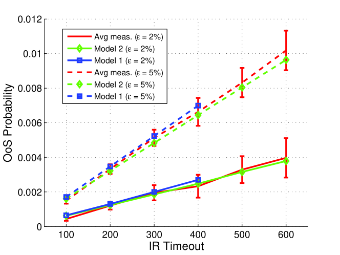
Figure 5: Comparison of the OoS probability against the IRT of the theoretical models and a ROHC implementation. $W=29$, $\epsilon=2\%$, $L_{B}=5$.

An important point is also how well the simplified model approximates the more sophisticated and realistic one. As stated, the purpose of the former is not to give an accurate numerical representation of the actual ROHC performance, but rather to foresee the trends up to a multiplicative constant. Fig. 6 shows the ratio of the OoS probabilities as predicted by the second and first models. It can be observed that the two models yield similar results (up to a multiplicative factor) for a wide range of design parameters. The multiplicative factor is mostly limited between 0.5 and 2, hence the simplified model still yields useful first order approximations of the OoS probability for many practically relevant values. The main reason why the results of the simplified approach deviate from those of Model 1 lie in the CRC check when the wraparound mechanism is applied. In Model 1 (as in the practical ROHC implementations), when the wraparound mechanism is employed, the decompressor may lose synchronization even if $w<W$. This fact is ignored by Model 2 and hence when $W$ is large the simplified approach underestimates the OoS probability, contrary to Model 1. We remark that for $W=29$ (widely employed in practice), the two models essentially yield the same prediction, and this is indeed the case in Fig. 5. Moreover, for large values of the IRT, the multiplicative factor depends very weakly on IRT and far more on $W$.

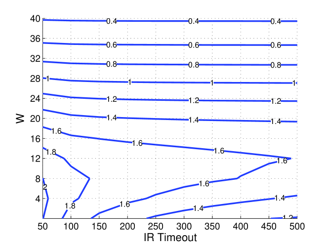
Figure 6: Contour plot of the ratio between the OoS probabilites of model 2 and model 1. $\epsilon=2\%$, $L_{b}=5$.

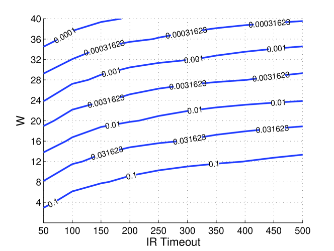
Figure 7: Contour plot of the OoS probability for the second model. $\epsilon=2\%$, $L_{b}=5$.

The previous graphs have demonstrated the validity of the proposed models. Fig. 7 represents the OoS probability for a range of IR timeout and interpretation window $W$ for model 2. The picture shows that for $W=29$ the OoS probability is below $0.3\%$, which is one order of magnitude smaller than the channel error rate ($2\%$), and with this choice of $W$ ROHC does not degrade appreciably the overall performance of the system compared to the errors intrinsically introduced by the channel. Instead, if the wraparound mechanism was not adopted, $W$ would drop to 13 and the OoS probability would soar to values between 1 and 10%; thus the ROHC mechanism could introduce more errors than the channel does and would become the limiting factor of the system performance. Therefore, the wraparound mechanism is necessary to provide satisfactory performance in correlated wireless channels. This statement is further supported by Fig. 8, which compares the OoS probability with and without wraparound against the average deletion probability for $L_{B}=5$. The necessity of this mechanism in order to extend $W$ to acceptable values is clear.

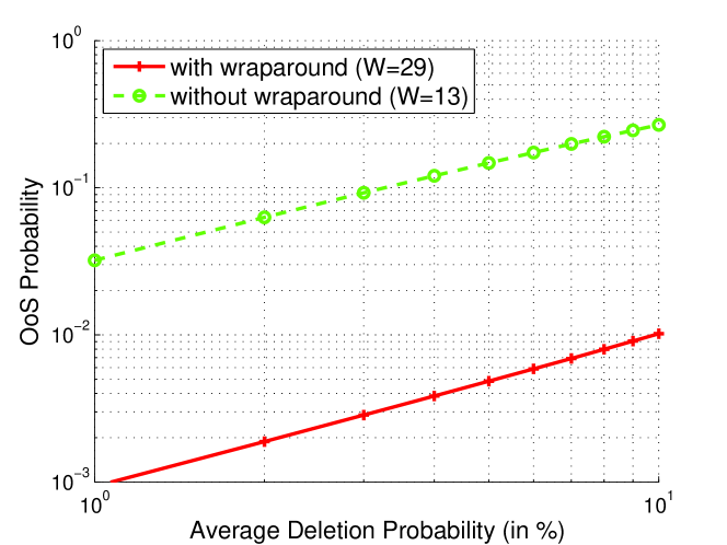
Figure 8: OoS probability of model 2 against the average erasure probability $\epsilon$ with and without wraparound. $L_{b}=5$, IRT = 300.

An important practical question is how the interpretation window $W$ should be tuned as the correlation time of the channel (exemplified by $L_{B}$) changes, for a given target of OoS probability. In particular, it was decided to target an OoS probability equal to 10% of $\epsilon$, so that ROHC is not the limiting factor in the system performance. The results are depicted in Fig. 9. The dependence between the error burst length and the minimum value of $W$ is approximately linear, which is in rough agreement with Eq. (18). The picture suggests that the interpretation interval $W$ should be about 5.5-6 times larger than the average burst length for the given target reliability and IR timeout, which is in agreement with the value suggested by Eq. (18).

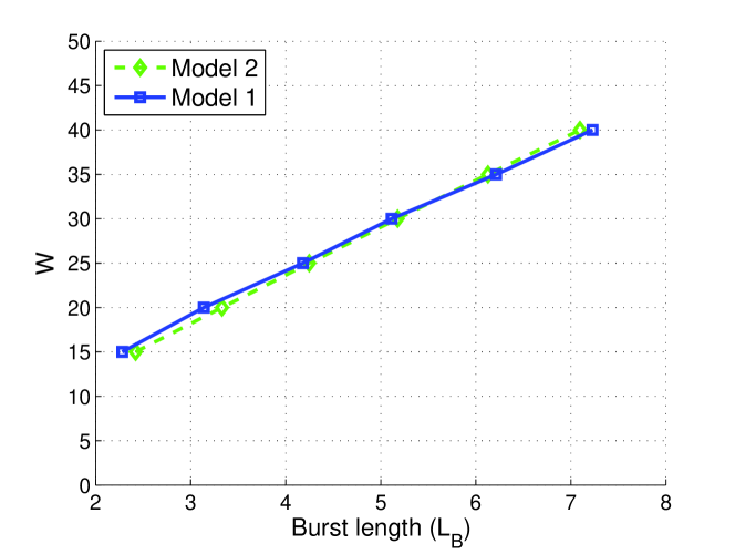
Figure 9: Minimum value of $W$ to achieve an OoS probability no larger than $\epsilon/10=0.2\%$ against the burst length $L_{B}$. $\epsilon=2\%$, IRT = 300.

A similar analysis has been carried out for the IR timeout changing as a function of $L_{B}$ (i.e., of the channel correlation) for a given target of OoS probability. The results are not reported due to limits of space, but it can be shown that the choice of the IRT is quite sensitive to the average burst length and it follows the approximately exponentially inverse relationship of Eq. (19). Moreover, the predictions of both models agree rather well with each other, which confirms the accuracy of the simplified approach.

While the OoS probability is a very important metric, ROHC must also provide sufficiently high compression efficiency. Fig. 10 shows the average compression efficiency when ROHC is run on IPv6 as a function of the average burst error length. This metric is defined as:

$$\mu=\frac{H_{IR}-E[H]}{H_{IR}}$$ (23)

where $H_{IR}$ is the length of an uncompressed header and $E[H]$ is the average length of a compressed header. This ratio measures the amount of spared bandwidth due to ROHC against the bandwidth required without this compression algorithm. The target OoS probability is $0.2\%$ and the IR timeout is set to 300 as in Fig. 9. The high compression effectiveness of ROHC is demonstrated by the ability to shrink the header by a factor of 16-20. As $L_{B}$ increases, the IRT must be decreased so as to cope with the increased channel correlation and therefore the compression efficiency is reduced, but a satisfactory factor of at least 15 can be attained in all cases.

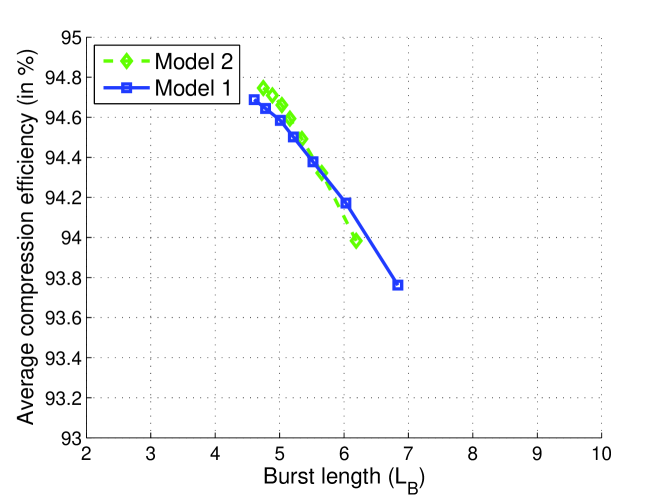
Figure 10: Compression efficiency against $L_{B}$. $\epsilon=0.2\%$, $W=29$.

The previous results concerned the single flow case. The last two plots explore the performance of the multi flow setting, which is inferred through the model of Section III-C. Fig. 11 shows the OoS probability against $M$ for IRT$\in\{100;300\}$. It is clear that an excessive number of flows eventually leads to an increase of the OoS probability, as the interpretation window of the IP identifier will be often crossed. Indeed, for $M\geq 3$, the performance degrades constantly as the number of flows is increased. On the other hand, multiplexing three flows together slightly improves the probability compared to having a single flow and with $M=2$ the effect is quite dramatic. The multiplexing of more flows together increases the time diversity and reduces the channel correlation, hence for $M=2$ the first effect (more time diversity) is dominant over the other consequence (increased vulnerability to interpretation window crossings) and the mechanism is even beneficial for small $M$. In our setting, for $M$ beyond 3 the average error burst length becomes smaller that the average time between two consecutive packets of the same IP flow. Hence, additional time diversity does not help as the channel is already sufficiently decorrelated. Fig. 12 shows the effect of the IP identifier interpretation interval $W_{o}$ for $M=3$. It is intuitive that the OoS probability worsens with the reduction of $W_{o}$. The picture shows in fact a very strong sensitivity with $W_{o}$ and suggests an inversely exponential dependence of the OoS probability with $W_{o}$, similar to what was observed for single IP flow profiles against $W$.

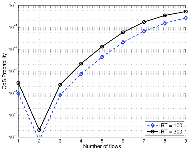
Figure 11: OoS probability against $M$ for two values of IRT. $W_{o}=47,\,W=62$, $\epsilon=2\%$, $L_{B}=5$.

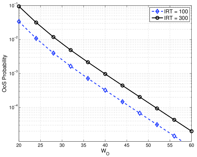
Figure 12: OoS probability against $W_{o}$ for two values of IRT. $W=62$, $\epsilon=2\%$, $L_{B}=5$.

V Conclusions

This paper has investigated a simple yet accurate model for the Robust Header Compression Protocol in deletion channels. Our work has shed light into the qualitative dependence of the system behavior as a function of the channel characteristics (coherence time and deletion probability) and the design parameters (IR timeout and the interpretation window $W$). The model encompasses also the practically relevant case of IP flow multiplexing and its predictions have been widely investigated over different scenarios. While this paper has investigated the U-mode, the introduction of a feedback channel in the O-mode and R-mode poses interesting questions from both a theoretical and practical point of view and deserves investigation.

VI Acknowledgments

The research leading to these results has been partially funded by the European Community’s Seventh Framework Programme (FP7/2007-2013) under Grant Agreement n° 233679. The SANDRA project is a Large Scale Integrating Project for the FP7 Topic AAT.2008.4.4.2 (Integrated approach to network centric aircraft communications for global aircraft operations).

The undetected error probability for the 3-bit ROHC CRC is with very good approximation 1/32, and it can be explained as follows. Since the ROHC CRC has a minimum distance of three, a possible configuration for undetected error is that the SN numbers (i.e., the systematic part) are different in three bits and the redundancy parts are equal. The most likely case to confuse the actual and reconstructed SNs is for them to be different in the three LSBs. Let us now assume that the two LSBs of the 12 context bits of the reconstructed SN are equal to 1 (which happens with probability 1/4). By definition, the true SN must be larger and the smallest number than can be added to the SN is clearly "one". The two LSBs must flip to zero, but the third bit switches as well due to the carry over. At least three bits are different and hence the CRC and the reconstructed SN may match. The CRC of this reconstructed SN is composed by 3 bits and is in general different from the original one, but there is a 1/8 chance that it is equal to the one sent in the compressed header, thus the overall CRC false negative probability of 1/32.

References

- [1] C. Bormann, C. Burmeister, M. Degermark, H. Fukushima, H. Hannu, L.-E. Jonsson, R. Hakenberg, T. Koren, K. Le, Z. Liu, A. Martensson, A. Miyazaki, K. Svanbro, T. Wiebke, T. Yoshimura, and H. Zheng, “IETF RFC 3095, Robust Header Compression (ROHC): Framework and four profiles: RTP, UDP, ESP, and uncompressed,” July 2001.
- [2] D.E. Taylor, A. Herkersdorf, A. Doring, and G. Dittmann, “Robust Header Compression (ROHC) in Next-Generation Network Processors,” IEEE/ACM Trans. Networking, vol. 13, no. 4, pp. 755–768, Aug. 2005.
- [3] G. Pelletier, L.-E. Jonsson, and K. Sandlund, “IETF RFC 4224, RObust Header Compression (ROHC): ROHC over Channels That Can Reorder Packets,” January 2006.
- [4] Effnet, “The Concept of robust header compression, ROHC,” White paper, February 2004.
- [5] M.A. West, L.W. Conroy, R.E. Hancock, R. Price, and A.H. Surtees, “IP header and signalling compression for 3G systems,” in 3G Mobile Communication Technologies, 2002, London (UK), May 2002.
- [6] S. Rein, F.H.P. Fitzek, and M. Reisslein, “Voice quality evaluation in wireless packet communication systems: a tutorial and performance results for RHC,” IEEE Wireless Commun. Mag., vol. 12, no. 1, pp. 60 – 67, Feb. 2005.
- [7] H. Wang, J.S. Li, and P.L. Hong, “Performance analysis of ROHC U-mode in wireless links,” Communications, IEE Proceedings-, vol. 151, no. 6, pp. 549–551, dec. 2004.
- [8] H. Woo, J. Kim, M. Lee, and J. M. Kwon, “Performance analysis of Robust Header Compression over mobile WiMAX,” in ICACT 2008, Peyongchang (Korea), Feb. 2008.
- [9] P. Fortuna, G. Carneiro, and M. Ricardo, “Robust header compression in 4G networks with QoS support,” in IEEE PIMRC 2005, Sept. 2005.
- [10] E. Piri, J. Pinola, F. Fitzek, and K. Pentikousis, “ROHC and aggregated VoIP over fixed WiMAX: An empirical evaluation,” in IEEE ISCC 2008, Marrakech (Morocco), July 2008.
- [11] H. Jin, R. Hsu, and Jun Wang, “Performance comparison of header compression schemes for RTP/UDP/IP packets,” in IEEE WCNC 2004, Atlanta (GA, USA), Mar. 2004.
- [12] S. Kalyanasundaram, V. Ramachandran, and L.M. Collins, “Performance Analysis and Optimization of the Window-Based Least Significant Bits Encoding Technique of ROHC,” in IEEE GLOBECOM 2007, Washington (DC, USA), Nov. 2007.
- [13] C. Y. Cho, Y. H. Chew, and W. K. G. Seah, “Modeling and Analysis of Robust Header Compression Performance,” in IEEE WoWMoM 2005, Taormina (Italy), June 2005.
- [14] A. Couvreur, L.-M. Le Ny, A. Minaburo, G. Rubino, B. Sericola, and L. Toutain, “Performance Analysis of a Header Compression Protocol: The ROHC Unidirectional Mode,” Telecommunication Systems, vol. 31, no. 1, pp. 85–98, Jan. 2006.
- [15] H. Wang and K. G. Seah, “An Analytical Model for the ROCH RTP Profile,” in IEEE WCNC 2004, Atlanta (GA, USA), Mar. 2004.
- [16] L. Badia, N. Baldo, M. Levorato, and M. Zorzi, “A Markov Framework for Error Control Techniques Based on Selective Retransmission in Video Transmission over Wireless Channels,” IEEE J. Select. Areas Commun., vol. 28, no. 3, pp. 488–500, Apr. 2010.
- [17] K. S. Zigangirov, “Sequential decoding for a binary channel with dropouts and insertions,” Problems of Inform. Transm., vol. 5, no. 2, pp. 17–22, 1969.
- [18] R. Hermenier, F. Rossetto, and M. Berioli, “A Simple Analytical Model for RObust Header Compression in Correlated Wireless Links,” ISWCS, 6-9 Nov 2011.
- [19] F. Calì, M. Conti, and E. Gregori, “Dynamic tuning of the IEEE 802.11 protocol to achieve a theoretical throughput limit,” IEEE/ACM Trans. Networking, vol. 8, no. 6, pp. 785–799, Dec. 2000.
- [20] S. S. Lam, Packet Switching in a Multi-Access Broadcast Channel with Application to Satellite Communication in a Computer Network, Ph.D. thesis, Department of Computer Science, University of California, Los Angeles, Mar. 1974.
- [21] Gradshteyn and Ryzhik, Table of Integrals, Series, and Products, Alan Jeffrey and Daniel Zwillinger (eds.) Seventh edition, 2007.
- [22] G. H. Golub and F. Van Loan, Matrix computations, Johns Hopkins University Press, Baltimore (MD, USA), 1996.
- [23] “The RObust Header Compresion (ROHC) library in Launchpad,” https://launchpad.net/rohc.