Analytic solution of a model of language competition with bilingualism and interlinguistic similarity

Abstract

An in-depth analytic study of a model of language dynamics is presented: a model which tackles the problem of the coexistence of two languages within a closed community of speakers taking into account bilingualism and incorporating a parameter to measure the distance between languages. After previous numerical simulations, the model yielded that coexistence might lead to survival of both languages within monolingual speakers along with a bilingual community or to extinction of the weakest tongue depending on different parameters. In this paper, such study is closed with thorough analytical calculations to settle the results in a robust way and previous results are refined with some modifications. From the present analysis it is possible to almost completely assay the number and nature of the equilibrium points of the model, which depend on its parameters, as well as to build a phase space based on them. Also, we obtain conclusions on the way the languages evolve with time. Our rigorous considerations also suggest ways to further improve the model and facilitate the comparison of its consequences with those from other approaches or with real data.

1 Introduction

At whatever scale that we look, languages reveal themselves as very elaborated entities consisting of many coupled parts: grammar, vocabulary, etc; each of them complex in its own nature as well. They are, moreover, a main instrument of interaction in an entangled web of social agents so that the state and evolution of tongues cannot, ultimately, be considered as detached from other social dynamics. We readily appreciate that we are in front of an utter challenge to the human intellect [1, 2]. Small steps are gradually taken towards a further understanding of the many problems posed by languages. Leaving aside those contributions from the more classic fields (e.g. philology), linguistic questions were opened to very diverse branches of science during the 20th century by drawing inspiration from some pioneer multi- disciplinary works [3]. Given the complexity outlined before, any of these first transversal approaches are necessarily simplistic or rely largely on computer simulations, and rigorous and definitive mathematical proofs of the results are often missing.

The kind of questions that were exposed to a more varied community of researchers regard the evolution of languages: transformations in their syntaxes, grammars, or vocabularies; aging, rise, and death; the dynamics of their number of speakers: spreading of culture, competition or other kind of interaction with other tongues; etc. And the fields that take on these issues are as diverse as sociology, biology, or physics. The science of complex systems should be highlighted because of its very clever usage of existing mathematical methods that stem mainly from statistical mechanics [4]. While also appraising other important contributions that widen our knowledge about the nature of human languages [6, 5, 7, 8, 9, 10, 11, 12], we shall focus on a seminal paper by Abrams and Strogatz [13] that prominently triggered research in its direction. For an exhaustive review on very varied related topics with up-to-date bibliography consult [14]; and for a more extended review on the impact of statistical physics on social dynamics, including language modeling, see [15].

The line of research propelled by [13] addresses the modeling of language coexistence as a competitive dynamics to attract speakers. In [13] a minimal model was accounted for and in accordance with experimental data a sounded result spread: that a two-languages competition for speakers always led to the extinction of one of the parties. Further analysis of the model [16, 17] shows that it also allows for stable language coexistence, but the parametric setup needed has not been observed in any study with available real data. Following the trend, more complicated models were developed that took spatial or social structure into account [18, 19, 20] or that explicitly introduced bilingualism [20, 21, 22, 23, 24, 25, 26]. This naturally eased the way to solutions with stable coexisting languages.

As it was advanced before, computer simulations constitute a favorite tool in this modern wave of scientific approaches to the study of languages. The results are usually convincing more than enough and, besides, these numerical studies allow to reach a depth of knowledge that might be impossible if we should rely only on very rigorous analytical demonstrations. Despite of this, many of the most insightful contributions to the comprehension of human communication follow from meticulous and carefully proven mathematical constructions, mainly in the study of grammars and largely aided by methods from computational sciences [27].

In this paper we intend to make a contribution by analytically elucidating some existing results in the modeling of language competition. This is necessarily a rearguard job–since computer simulations have the lead by far–but we will see how it is very valuable and necessary. Thanks to the thorough reasoning of this paper we gain a deep understanding about the dynamics of speakers of coexisting languages. We focus on a model of language competition that allows bilingualism introduced in [23] and whose most interesting results were numerically derived in [25]. By analyzing the model we will come to a better interpretation of the previous numerical work and we will reach some new results that are, now, supported by robust analytical proofs.

The paper is structured in the following way: In section 2 the hypothesis used in [23] are formulated and the corresponding equations are derived therefrom. In section 3 strict mathematical results are carefully obtained. Whenever the analytic tools do not reach to fully solve the problem, numerical simulations are employed, but its presence–usually at the very end of the chain of reasoning–is always warned to the reader to leave any minimally uncertain result open to debate. In section 4 the more mathematical aspects of the reached solutions are left aside and the results are analyzed primarily from the point of view of language dynamics: what does the analytical outcome mean in terms of coexisting languages?

2 Derivation of the model equations

Closely following the path pointed out by Abrams and Strogatz [13], we work on a model of two competing languages where bilingualism is an option in between and where the similarity between the tongues plays and explicit role [23]. The model considers a human population whose individuals might talk either of two languages $X$ or $Y$ or both of them. Along the text we might refer to either of the monolingual communities or the bilingual one as groups, standing for groups of speakers. Naming $x$ and $y$ the fraction of monolingual speakers of each tongue, and naming $b$ the fraction of bilingual speakers; two non- linear coupled differential equations are derived from the following basic hypothesis:

1. Population size remains constant.

2. The probability that an individual acquires a language different from its current one grows with the status of the new language. Therefore a status parameter $s\in[0,1]$ of one of the languages is introduced (being $1-s$ the status of the other one). These statuses are constant and a property of the system of coexisting languages.

3. It is possible to define a distance between two languages. This was done in [23] introducing a parameter called interlinguistic similarity, $k\in[0,1]$: $k=0$ for orthogonal languages, $k=1$ for exactly equal languages–a measure of how close the languages are to each other. This allowed to get this distance in an easy and straight way, by simply fitting percentages of speakers of the involved languages along time to a set of differential equations. This interlinguistic similarity is constant and, again, a property of each pair of languages. This parameter describes how difficult it is for a monolingual speaker to learn the other language: this task should be easier if the languages are more similar to each other. Another view of it is that the probability that an individual retains its old language when learning a new one grows with this parameter $k$. Thus, the parameter $k$ is the gate which opens the way to the birth of a bilingual group.

4. The probability that an individual acquires a language different from its current one grows with the fraction of speakers of the new language. An exponent $a$ is introduced to ponder the importance of the fraction of speakers in a group in attracting new speakers with respect to $s$ and $k$. Once more, $a$ should be a constant that characterizes each system of two competing languages. Existing field work with similar equations [13] shows that the equivalent parameter in that model varies little across pairs of coexisting languages, suggesting that social pressure to shift languages might be a constant through cultures.

Considering different hypothesis or variations on the implementation of the current ones might lead to different modeling of the same phenomenon [21, 22, 24]. In the present paper we focus on this minimal model whose results could be compared to data from a real system where the hypotheses are reasonably met [23, 25].

As stated previously, we seek to analytically solve the model introduced in [23] and test the consistence of the results obtained in [25]. Therefore we will be working on the set of differential equations that the authors derived for the dynamics of the fraction of monolingual speakers of each language. The derivation is as follows:

We formulate the probability of shifting languages $P_{XY}$ and $P_{YX}$ and the probability of arriving to (departing from) the bilingual group from each monolingual group $P_{XB}$, $P_{YB}$ ($P_{BX}$, $P_{BY}$) based on the hypothesis listed above:

$$P_{XB} = ck(1-s)(1-x)^{a},$$

$$P_{YB} = cks(1-y)^{a},$$

$$P_{BX}=P_{YX} = c(1-k)s(1-y)^{a},$$

$$P_{BY}=P_{XY} = c(1-k)(1-s)(1-x)^{a}.$$ (1)

$c>0$ is a normalization constant [25]. Equations 1 are used to reckon the rates at which the population of the three groups grow or decline:

$${dx\over dt} = F_{x}(x,y),$$

$${dy\over dt} = F_{y}(x,y).$$ (2)

A third differential equation exists that tracks the evolution of the proportion $b$ of bilinguals, but this will not be needed in the following thanks to the normalization of the population $x+y+b=1$. In [25] these equations are written such that the contributions of all terms from equations 1 can be explicitly read, but here we prefer a more compact notation so that we can research the field $F=(F_{x},F_{y})$:

$$F_{x}(x,y) = c\left[(1-x)(1-k)s(1-y)^{a}-x(1-s)(1-x)^{a}\right],$$

$$F_{y}(x,y) = c\left[(1-y)(1-k)(1-s)(1-x)^{a}-ys(1-y)^{a}\right].$$ (3)

For the present study, the parameters are restricted to $k\in(0,1)$, $s\in(0,1)$, and $a>0$. Sometimes $a$ will be further restricted. If this is the case, it will be noted.

As said before, the parameter $c$ normalizes the dynamics and is irrelevant for equilibrium points and stability issues, therefore it was not paid much attention in previous literature and neither will it be paid attention now. The parameter $a$ generalizes the monotonously increasing dependence of the probability of transition between languages as outlined in the fourth hypothesis. This parameter has been found to be larger than $1$ and relatively constant among cultures ($a\sim 1.31$) in experimental accounts of the problem of language dynamics [13, 23, 25], but we intend to address the behavior of the system for $a>0$, which is a more interesting generalization. The other parameters that concern us are $k$ and $s$.

3 Resolution of the model

3.1 The model yields realistic trajectories

We note that all the possible distributions of speakers among the different groups can be represented in the $x-y$ space. There, the condition $x+y+b=1$ defines a triangular set $A=\{(x,y),\>\>x\geq 0,y\geq 0,x+y\leq 1\}$ upon which the fields $F_{x}(x,y)$ and $F_{y}(x,y)$ are acting. For the sake of basic consistency of the model, its solutions must be feasible; meaning that a negative number of individuals in any group should be forbidden: the dynamics must happen inside $A$ for realistic systems.

Lemma 3.1

Assume the parameter $a>0$. The set $A=\{(x,y),\>\>x\geq 0,y\geq 0,x+y\leq 1\}$ is positive invariant.

• Let us see that the field defined in equations 3 is directed inwards in the boundaries of $A$.

  1. If $x=0$ and $y\in[0,1]$:

     $$F_{x}(0,y) = c(1-k)s(1-y)^{a}\geq 0,$$

     $$F_{y}(0,y) = c\left[(1-y)(1-k)(1-s)-ys(1-y)^{a}\right].$$ (4)

     The first inequality implies that the field flows inwards $A$ since $F_{x}(0,y)\geq 0$ for $0\leq y\leq 1$.

  2. If $y=0$ and $x\in[0,1]$:

     $$F_{x}(x,0) = c\left[(1-x)(1-k)s-x(1-s)(1-x)^{a}\right],$$

     $$F_{y}(x,0) = c(1-k)(1-s)(1-x)^{a}\geq 0.$$ (5)

     For $y=0$ the field flows inwards $A$ since $F_{y}(x,0)\geq 0$ for any $0\leq x\leq 1$.

  3. If $y=1-x$:

     $$F_{x}(x,1-x) = c\left[(1-x)(1-k)sx^{a}-x(1-s)(1-x)^{a}\right],$$

     $$F_{y}(x,1-x) = c\left[x(1-k)(1-s)(1-x)^{a}-(1-x)sx^{a}\right].$$ (6)

     In this case the field flows inwards $A$ if and only if $-F_{x}(x,1-x)-F_{y}(x,1-x)\geq 0$ since $(-1,-1)$ is a normal vector to the straight line $y=1-x$ pointing towards the interior of $A$. That condition is trivially satisfied and we conclude again that the field flows inwards into $A$ through the segment $y=1-x$, $x\in(0,1)$.

This lemma means that any real distribution of speakers between the available groups that would evolve according to the proposed equations would remain feasible all the time.

3.2 Number of fixed points of the dynamics in $A$

It is possible to find upper and lower limits to the number of equilibrium points that the system displays for different $k$, $s$, and $a$. We find the equilibrium point of the system wherever the nullclines (curves defined by $dx/dt=0$ and $dy/dt=0$) intersect each other. In $A$, the equilibrium points that can be detected by a simple inspection of the system are $P_{x}=(1,0)$ and $P_{y}=(0,1)$. We will term them trivial fixed points. There is another trivial fixed point for the dynamics, but it lays outside $A$: the point $(1,1)$. Depending on different values of the mentioned parameters we shall find more equilibrium points inside $A$. Following the notation introduced in this paragraph, we appreciate that the curves $x=1$ and $y=1$ are branches of the nullclines of the system. We name them the trivial branches. Our analysis will deal mainly with the non trivial branches.

With a preliminary analysis of the nullclines of the field ($F_{x}=0$, $F_{y}=0$) it is possible to narrow down the number of fixed points in the interior of $A$ to a maximum of $3$: Equilibrium points of the dynamics are found in the intersections of the nullclines. Equating both components of the field to zero we get:

$$(1-y)^{a} = {1-s\over s}{1\over 1-k}x(1-x)^{a-1},$$

$$(1-x)^{a} = {s\over 1-s}{1\over 1-k}y(1-y)^{a-1}.$$ (7)

Multiplying these equations and isolating $y$:

$$y={1\over 1+{x\over(1-k)^{2}(1-x)}}.$$ (8)

We must restrict ourselves to $x\neq 1\neq y$ now to avoid divergences here and in following equations, but this is enought to continue with our discussion.

Substituting equation 8 into the second expression of equations 7:

$$(1-x)^{a} = {s(1-k)(1-x)\over(1-s)x}\left(1-{1\over 1+{x\over(1-k)^{2}(1-x)}}\right)^{a}\Rightarrow$$ (9)

$$\Rightarrow \left(1-x\over x\right)^{a-1}\left(x+(1-k)^{2}(1-x)\right)^{a}={s\over 1-s}(1-k).$$

If $(x^{*},y^{*})$ is an equilibrium point, $x^{*}$ must obey equation 9 and the corresponding $y^{*}$ is obtained from equation 8.

From the left-hand side of equation 9:

$$g(x) \equiv \left(1-x\over x\right)^{a-1}\left(x+(1-k)^{2}(1-x)\right)^{a}.$$ (10)

If $a>1$ it is true that:

$$g(x) > 0,\>\>\>\>\forall x\in(0,1);$$

$$\lim_{x\to 0^{+}}g(x) = +\infty;$$

$$\lim_{x\to 1^{-}}g(x) = 0.$$ (11)

Furthermore, $g(x)$ has got a relative minimum and a relative maximum respectively at:

$$x^{-} = {1\over 2a}\left(1-\sqrt{1-{4a(a-1)(1-k)^{2}\over 2k-k^{2}}}\right)\in(0,1),$$

$$x^{+} = {1\over 2a}\left(1+\sqrt{1-{4a(a-1)(1-k)^{2}\over 2k-k^{2}}}\right)\in(0,1).$$ (12)

Because all of this, the equation $g(x)={s\over 1-s}(1-k)$ can only have one, two, or three solutions in $x\in(0,1)$ for fixed $k$ and $s$, restricting thus the number of equilibrium points of the whole system.

For $a=1$, $g(x)$ reduces to a straight line that might or might not fulfill $g(x)={s\over 1-s}(1-k)$ within the range of interest $x\in(0,1)$. Because $g(x)$ is a straight line, this equality can be obeyed for just one value of $x$ at most. Thus for $a=1$ there is at most one more fixed point within $A$, but it must not necessarily exist.

Finally, for $a<1$ the limits found in equation 11 swap:

$$\lim_{x\to 0^{+}}g(x) = 0,$$

$$\lim_{x\to 1^{-}}g(x) = +\infty;$$ (13)

and $g(x)>0$ in the whole range $x\in(0,1)$. It is also monotonically increasing within this range and thus must always match ${s\over 1-s}(1-k)$ in exactly one point $x^{*}$ internal to $A$. So for $a<1$ there is always one fixed point besides the trivial ones.

3.3 Stability of the equilibrium points $P_{x}=(0,1)$ and $P_{y}=(1,0)$ for $a>1$

We assess the stability of the system by evaluating the matrix at the existing fixed points, diagonalizing it, and considering the sign of the eigenvalues. For non trivial equilibrium points it becomes complicated to exactly locate them on the $x-y$ plane, left asside its analysis through the Hessian matrix; but for $P_{x}$ and $P_{y}$ and restricting ourselves to $a>1$ we can evaluate the Hessian matrix explicitly and it happens to be diagonal already:

$$DF(0,1) = \left(\begin{array}[]{cc}-c(1-s)&0\\ 0&-c(1-k)(1-s)\end{array}\right),$$ (16)

$$DF(1,0) = \left(\begin{array}[]{cc}-c(1-k)s&0\\ 0&-cs\end{array}\right).$$ (19)

Furthermore, the eigenvalues are negative meaning that $P_{x}$ and $P_{y}$ are asymptotically stable independently of the values of $k$ and $s$ for $a>1$.

Because $P_{x}$ and $P_{y}$ are always stable for $a>1$ and the field is such that all trajectories enter $A$, if there is only one more equilibrium point $x^{*}$ interior to $A$ it must be a saddle point and lie exactly at the frontier between the basins of attraction of $(0,1)$ and $(1,0)$. If $x^{*}$ were unstable yet not a saddle point, either there would exist two more fixed points where the boundaries between basins cross the frontier of $A$, or there would exist trajectories leaving $A$; and neither of these is the case. If $x^{*}$ were stable it would have a basin of attraction for itself and new fixed points would need to exist in the separation between different basins.

3.4 Studying the field in different regions of $A$ for $a>1$

Now we will get more insights about the dynamics by further characterizing the field $F$ at the boundary of $A$ and in its interior. For this analysis we must assume $a>1$, otherwise some of the functions that we will be making use of will be ill-defined.

3.4.1 Studying $F$ at the boundary of $A$

Recalling $F_{y}(0,y)$ from equation 4, we introduce:

$$G_{y}(y) \equiv (1-k)(1-s)-ys(1-y)^{a-1},$$ (20)

and we note that it is continuous on the interval $[0,1)$, strictly decreasing on $(0,1/a)$ and strictly increasing on $(1/a,1)$. Since:

$$G_{y}(0)=G_{y}(1) = (1-k)(1-s)>0,$$ (21)

we can find out if this function ever changes its sign by evaluating it at its minimum: $G_{y}(1/a)$. We get either:

$${(a-1)^{a-1}\over a^{a}} < (1-k){1-s\over s},$$ (22)

which would imply that $F_{y}(0,y)>0\>\>\forall y\in[0,1)$; or:

$${(a-1)^{a-1}\over a^{a}} \geq (1-k){1-s\over s},$$ (23)

which would imply that there would exist $y_{1},y_{2}\in(0,1)$ such that $F_{y}(0,y)>0$ if $y\in[0,y_{1})\cup(y_{2},1]$ and $F_{y}(0,y)<0$ for all $y\in(y_{1},y_{2})$. In this case $F_{y}$ is zero at $(0,y_{1})$ and $(0,y_{2})$. Let us note that $y_{1}=y_{2}$ if the equality holds on equation 23.

Likewise, recalling $F_{x}(x,0)$ from equation 5, we define:

$$G_{x}(x) \equiv (1-k)s-x(1-s)(1-x)^{a-1},$$ (24)

which is continuous on $x\in[0,1)$, strictly decreasing on $(0,1/a)$ and strictly increasing on $(1/a,1)$. Also:

$$G_{x}(0)=G_{x}(1) = (1-k)s>0,$$ (25)

thus we find either:

$${(a-1)^{a-1}\over a^{a}} < {s\over 1-s}(1-k),$$ (26)

which would imply $F_{x}(x,0)>0\>\>\forall x\in[0,1)$; or:

$${(a-1)^{a-1}\over a^{a}} \geq {s\over 1-s}(1-k),$$ (27)

which would imply that there would exist $x_{1},x_{2}\in(0,1)$ such that $F_{x}(x,0)>0$ if $x\in[0,x_{1})\cup(x_{2},1]$ and $F_{x}(x,0)<0$ for all $x\in(x_{1},x_{2})$. In this case $F_{x}$ is zero at $(x_{1},0)$ and $(x_{2},0)$. Once again: $x_{1}=x_{2}$ if the equality holds on equation 27.

Let us note that if the strict inequalities 22 and 27 are simultaneously true then $s<1/2$ and if the strict inequalities 23 and 26 are simultaneously true then $s>1/2$.

On the diagonal $x+y=1$ the field takes the form written in equation 6 and the signs of $F_{x}(x,1-x)$ and $F_{y}(x,1-x)$ can be studied analyzing $\left({1-x\over x}\right)^{a-1}$ and $\left({x\over 1-x}\right)^{a-1}$ respectively:

Since the function $\left({1-x\over x}\right)^{a-1}$ is strictly decreasing on $(0,1)$ and:

$$\lim_{x\to 1^{-}}\left({1-x\over x}\right)^{a-1} = 0,$$

$$\lim_{x\to 0^{+}}\left({1-x\over x}\right)^{a-1} = +\infty;$$ (28)

then there exists only one $z_{x}\in(0,1)$ such that $\left({1-z_{x}\over z_{x}}\right)^{a-1}=(1-k){s\over 1-s}$ for fixed $k$ and $s$. Therefore $F_{x}(x,1-x)<0$ if $x\in(0,z_{x})$ and $F_{x}(x,1-x)>0$ if $x\in(z_{x},1)$.

With a similar argument for $\left({x\over 1-x}\right)^{a-1}$ it can be warranted the existence of only one $z_{y}\in(0,1)$ such that $\left({z_{y}\over 1-z_{y}}\right)^{a-1}=(1-k){1-s\over s}$ for fixed $k$ and $s$. Then $F_{y}(x,1-x)>0$ if $x\in(0,z_{y})$ and $F_{y}(x,1-x)<0$ if $x\in(z_{y},1)$.

It can be trivially shown that $z_{y}<z_{x}$. Also it is true that $\left|F_{x}(x,1-x)\right|>F_{y}(x,1-x)$ if $x\in(0,z_{y})$ and $F_{x}(x,1-x)<\left|F_{y}(x,1-x)\right|$ if $x\in(z_{x},1)$.

3.4.2 Further study of $F_{x}$

If $x\neq 0$ and $x\neq 1$, then the points $(x,y)$ which nullify the first component of the field $F$ are those that obey:

$$y = 1-\left({1-s\over s}\right)^{1/a}{1\over(1-k)^{1/a}}x\left({1-x\over x}\right)^{1-1/a}.$$ (29)

The function $h_{x}:[0,1]\rightarrow\mathbb{R}$ is defined as:

$$h_{x}(x) = 1-\left({1-s\over s}\right)^{1/a}{1\over(1-k)^{1/a}}x\left({1-x\over x}\right)^{1-1/a}$$ (30)

on $x\in(0,1]$ and $h_{x}(0)=1$. It is strictly decreasing on $(0,1/a)$ and increasing on $(1/a,1)$, it has got a minimum at $1/a$, and $h_{x}(0)=1=h_{x}(1)$.

If $y<h_{x}(x)$ then $F_{x}(x,y)>0$. If $y=h_{x}(x)$ then $F_{x}(x,y)=0$. If $y>h_{x}(x)$ then $F_{x}(x,y)<0$.

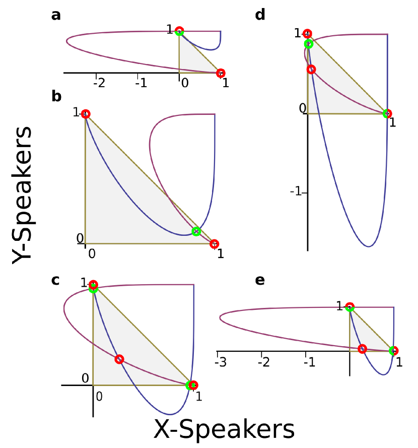
Figure 1: Non-trivial nullclines of the system for different values of $k$ and $s$ and fixed $a=1.31$. Five pairs of parameters $(k,s)$ were used to plot the non-trivial branches of the nullclines. The values were chosen to compare our results with those from [25], thus: a $k=0.65$, $s=0.80$, b $k=0.20$, $s=0.40$, c $k=0.65$, $s=0.50$, d $k=0.75$, $s=0.35$, and e $k=0.75$, $s=0.35$. Stable fixed points are indicated in red and saddle points in green. Contrary to what was interpreted in [25], cases a and b on one side and c, d, e on the other side are equivalent to each other. The five differentiated cases are obvious, though, if we attend to the sizes of certain basins of attraction: some of them can hardly be detected with numerical systems. We can appreciate in the different figures how important features, like crossings with the boundary evolve for the different parameters. This can be better grasped in [28].

If the parameters of the system are such that inequality 26 holds, then $h_{x}(1/a)>0$ and the plot of $h_{x}(x)$ intersects the boundary of $A$ at $(0,1)$ and $(z_{x},1-z_{x})$ (figs. 1a-b).

If the strict inequality 27 holds true then $h(1/a)<0$ and the plot of $h_{x}(x)$ intersects the boundary of $A$ at $(0,1)$, $(x_{1},0)$, $(x_{2},0)$, and $(z_{x},1-z_{x})$ (figs. 1c-e).

Additionally, since $F_{y}(x_{2},h_{x}(x_{2}))>0$ and $F_{y}(z_{x},h_{x}(z_{x}))<0$, because $F_{y}$ and $h_{x}$ are continuous, it is warranted the existence of $p\in(x_{2},z_{x})$ such that $F(p,h_{x}(p))=(0,0)$ –i.e. a fixed point of $F$.

3.4.3 Further study of $F_{y}$

If $y\neq 0$ and $y\neq 1$, then the points $(x,y)$ which nullify the second component of the field $F$ are those which obey:

$$x = 1-\left(s\over 1-s\right)^{1/a}{1\over(1-k)^{1/a}}y^{1/a}(1-y)^{1-1/a}.$$ (31)

We define $h_{y}(y)$ similarly as we defined $h_{x}(x)$. This function is strictly decreasing on $(0,1/a)$ and increasing on $(1/a,1)$, and $h_{y}(0)=1=h_{y}(1)$.

If inequality 22 holds true then $h_{y}(1/a)>0$ and the curve $\{(h_{y}(y),y),y\in[0,1]\}$ intersects the boundary of $A$ at $(1,0)$ and $(z_{y},1-z_{y})$ (fig. 1b).

If the strict inequality 23 holds true then $h_{y}(1/a)<0$ and the curve $\{(h_{y}(y),y),y\in[0,1]\}$ intersects the boundary of $A$ at $(1,0)$, $(0,y_{1})$, $(0,y_{2})$, and $(z_{y},1-z_{y})$ (figs. 1a, and 1c-e).

Additionally, since $F_{x}(h_{y}(y_{2}),y_{2})>0$ and $F_{x}(h_{y}(1-z_{y}),1-z_{y})<0$, because $F_{x}$ and $h_{y}$ are continuous, it is warranted the existence of $q\in(y_{2},1-z_{y})$ such that $F(h_{y}(q),q)=(0,0)$ –i.e. a fixed point of $F$.

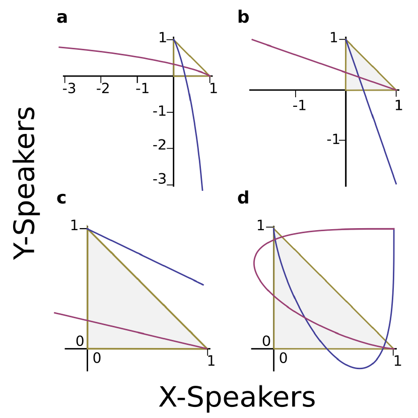
Figure 2: Non-trivial nullclines of the system for different values of $a$. Fixed $k=0.65$ and $s=0.50$ is taken except in panel c. This figure illustrates how the non- trivial branches of the nullclines suffer a sudden change as the parameter $a$ starting from $a<1$ increases through $a=1$ and to $a>1$. a For $a<1$ the nullclines must always cross inside $A$. b $a=1$ is the only case when the nullclines are straight lines that go through $(0,1)$ and $(1,0)$ respectively. As straight lines, depending on their slopes they might cross inside $A$, but this is not necessarily the case (c $a=1$, $k=0.3$, and $s=0.75$). d For $a>1$ the shape of the nullclines becomes more complicated and the possible crossings must be carefully addressed. We saw the many possibilities in fig. 1.

The evolution of both $h_{x}(x)$ and $h_{y}(y)$ as a function of the parameters $a$, $s$, and $k$ is partially shown in figs. 1 and 2, and can be dynamically explored in [28].

3.5 The nature of the orbits help us assess the stability of non-trivial fixed points

The nullclines are always landmarks of the dynamic system under research. Their obvious use is to locate the equilibrium points in their intersections, but more information can be extracted if we look at them carefully. In section 3.4 we used them to find out how the field behaves in the boundaries of $A$ as they mark the sets of points where the vertical and horizontal components of the field are nullified. This applies also in the interior of $A$: The trajectories of the system pass by with vertical tangent through the points of the curve $F_{x}(x,y)=0$, and with horizontal tangent through the points of the curve $F_{y}(x,y)=0$. But also, these curves divide $A$ in regions within which the signs of $F_{x}$ and $F_{y}$ are well determined. Topological arguments regarding the action of $F$ upon these different regions of $A$ help us put some limits to the kind of orbits that the system can yield: we will see that periodic dynamics can be banned. These considerations also let us find out whether non-trivial points are stable or not for $a>1$.

In this range of $a$ the system will always have at least one more equilibrium point in the interior of $A$. We have seen that this can be deduced either from the crossings of $h_{x}(x)$ and $h_{y}(y)$ with the boundary of $A$ or from equation 9 attending to the shape of $g(x)$. The analysis of $g(x)$ let us further know that also two or at maximum three fixed points can exist inside $A$. These three, two, or one equilibrium points will show up depending on the values of the parameters $s$, $k$, and $a$. Many possibilities are illustrated in fig. 1 and in [28].

With this in mind, let us consider the following regions:

$$R_{1} = \{(x,y)\in A/F_{x}(x,y)<0,F_{y}(x,y)>0\},$$

$$R_{2} = \{(x,y)\in A/F_{x}(x,y)>0,F_{y}(x,y)<0\}.$$ (32)

Equivalently:

$$R_{1} = \{(x,y)\in A/x\leq h_{y}(x),y\geq h_{x}(x)\},$$

$$R_{2} = \{(x,y)\in A/x\geq h_{y}(x),y\leq h_{x}(x)\}.$$ (33)

In a similar way we could introduce:

$$B_{1} = \{(x,y)\in A/F_{x}(x,y)>0,F_{y}(x,y)>0\},$$

$$B_{2} = \{(x,y)\in A/F_{x}(x,y)<0,F_{y}(x,y)<0\};$$ (34)

but these will not be interesting for us right now.

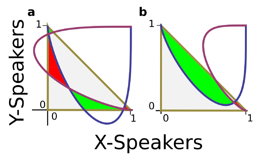
Figure 3: Positive invariant regions $R_{1}$ and $R_{2}$ on the $x-y$. We identify $R_{1}$, where $F_{x}$ is negative and $F_{y}$ is always positive (green in the figure); and $R_{2}$, where $F_{x}$ is positive and $F_{y}$ is negative (red regions). a $a=1.40$, $s=0.50$, $k=0.65$. Three equilibrium points exist inside $A$ and regions $A_{3}$ and $A_{4}$ are non-empty. Both $R_{1}$ and $R_{2}$ present two connected components ($A_{1}$ and $A_{3}$, and $A_{2}$ and $A_{4}$ respectively) which are, each of them, positive invariant. This means that the dynamics do not exit any of these regions once they enter: they must tend to a stable fixed point in their boundary. Thus, we see how points inside $A_{1}$ are taken to $P_{y}$ and points inside $A_{2}$ are taken towards $P_{x}$. The only possibility for regions $A_{3}$ and $A_{4}$ is that it exists another stable fixed points exactly in the joint between the two of them. b $a=1.31$, $k=0.20$, $s=0.40$. In this case only one equilibrium point exists inside $A$. Regions $A_{3}$ and $A_{4}$ are empty, but the same as before applies to regions $A_{1}$ and $A_{2}$: points in their interior must be driven towards $P_{y}$ and $P_{x}$ respectively.

Focusing on $R_{1}$ and $R_{2}$, they have got one or two connected components depending on if inside $A$ there exist one, two, or three equilibrium points. We shall write $R_{1}=A_{1}\cup A_{3}$, $R_{2}=A_{2}\cup A_{4}$; being $A_{3}$ or $A_{4}$ empty if on the interior of $A$ there are not three equilibrium points, and $A_{1}$ and $A_{2}$ the regions whose boundaries contain respectively $P_{y}=(0,1)$ and $P_{x}=(1,0)$. An account of these regions for some values of the parameters can be seen in fig. 3.

Taking into account the sign of the components of the field we can tell that regions $A_{1}$, $A_{2}$, $A_{3}$, and $A_{4}$ are positive invariant. If $(x_{0},y_{0})\in A_{1}$ then its trajectory $(x(t),y(t))$ for $t\in I_{t}[0,\infty)$ lays in $A_{1}$ because in the boundary of $A_{1}$ the field points inwards. This trajectory is thus contained in a compact for $t\in I_{t}$. Also, since ${dx(t)\over dt}<0$ and ${dy(t)\over dt}>0$, it can be verified that $x(t)$ is monotonously decreasing on $I_{t}$ and $y(t)$ is monotonously increasing on $I_{t}$. Consequently it exists the limit $\lim_{t\to+\infty}(x(t),y(t))=P_{y}$. The set $A_{1}$ is therefore contained in the basin of attraction of $P_{y}$. Analogously, it can be shown that if $(x_{0},y_{0})\in A_{2}$ then $\lim_{t\to+\infty}(x(t),y(t))=P_{x}$: its trajectory lays in the region of attraction of $P_{x}$; thus, the basin of attraction of $P_{x}$ contains $A_{2}$.

Also, if $A_{3}$ and $A_{4}$ are both non-empty and $(x_{0},y_{0})\in A_{3}\cup A_{4}$ its trajectory remains either inside $A_{3}$ or inside $A_{4}$ and converges towards the equilibrium point at the intersection of the frontiers of these regions. Since $A_{3}$ and $A_{4}$ are non-empty only when there are three equilibrium points inside $A$, this result means that one of these three points, whenever they exist, must be stable. In this case we can determine that the two remaining fixed points in the interior of $A$ must be saddle points. We do so with an argument similar to the one we used to show that $x^{*}$ is a saddle point when only one equilibrium point exists inside $A$ (section 3.3). We further deduce that the case with two interior fixed points corresponds to a saddle-node bifurcation and that this situation is the frontier between those cases with one and three equilibrium points in the space of parameters $k-s$.

Concerning the dynamics of the system, it is important the following lemma which ensures that there is no oscillatory behavior:

Lemma 3.2

There are not any periodic orbits in the x-y plane.

• Actually, because of the regularity of the field, applying the Poincaré-Bendixson theorem it can be deduced that if there would exist any closed orbit it must enclose a fixed point on its interior. Thus, the periodic orbit would necessarily enter and exit two of the regions $A_{i}$. This cannot happen because all regions $A_{i}$ are positive invariant.

This same argument also implies that fixed points cannot be foci, because trajectories approaching them should cross many times the frontiers between regions, some of which are positive invariant and cannot be left.

3.6 Tentative solutions for $a\leq 1$

Splitting the problem in $a>1$ on the one side and $a\leq 1$ on the other made its solution easier because several of the reasonings that work very well in the former case are built on functions that are ill-defined in the later. An example are the functions $G_{x}(x)$ and $G_{y}(y)$, but also the Hessian matrix in $(1,0)$ and $(0,1)$ present some problems for $a<1$. Luckily enough, in section 3.2 we proved that there is just one more equilibrium point $(x^{*},y^{*})$ for $a\leq 1$ which always appears if $a<1$ and that might not appear for $a=1$ depending on the parameters, so we do not need to investigate $3$ prospective fixed points as for $a>1$. Also it is still valid the demonstration that $A$ is positive invariant made in section 3.1.

In fig. 2 the nullclines are represented for various values of $a$ and fixed $k$ and$s$. We can observe $(x^{*},y^{*})$ in the intersections, and we can also observe how the nullclines suffer a deep transformation as values of $a$ larger than $1$ are employed. We shall study now the cases $a=1$ and $a<1$. Because of the analytic results are not so satisfactory, we shall complement them using numerical simulations whenever it is useful. These results should be questioned as long as a complete mathematical proof is not available.

It is particularly illustrative the resolution of the stability of $P_{x}=(1,0)$ and $P_{y}=(0,1)$ for $a=1$. This can still be analytically done. The Hessian matrix in this case reads:

$$DF(0,1) = \left(\begin{array}[]{cc}-c(1-s)&-c(1-k)s\\ 0&-c(1-k)(1-s)+cs\end{array}\right),$$ (37)

$$DF(1,0) = \left(\begin{array}[]{cc}-c(1-k)s+c(1-s)&0\\ -c(1-k)(1-s)&-cs\end{array}\right).$$ (40)

The eigenvalues are $\lambda_{P_{y}}^{1}=-c(1-s)$ and $\lambda_{P_{y}}^{2}=-c(1-k)(1-s)+cs$ for $P_{y}$ and $\lambda_{P_{x}}^{1}=-c(1-k)s+c(1-s)$ and $\lambda_{P_{x}}^{2}=-cs$ for $P_{x}$. We see that one of the eigenvalues is always the sum of two terms with different sign and this compromises the stability of $P_{x}$ and $P_{y}$. Indeed, their stability depends now on the parameters $k$ and $s$. By equating the conflictive terms to zero we obtain two curves relating $k$ and $s$:

$$s_{P_{y}} = {1-k_{P_{y}}\over 2-k_{P_{y}}},$$

$$s_{P_{x}} = {1\over 2-k_{P_{x}}}.$$ (41)

These curves tell us where does the stability of $P_{x}$ and $P_{y}$ change in the space of parameters $k-s$: $P_{x}$ is stable for $s>s_{P_{x}}$ and $P_{y}$ is stable for $s<s_{P_{y}}$. There is a region of values $s_{P_{y}}<s<s_{P_{x}}$ where neither $P_{x}$ nor $P_{y}$ are stable and, since there are not any trajectories leaving $A$, there must exist a point $(x^{*},y^{*})$ interior to $A$ that is stable.

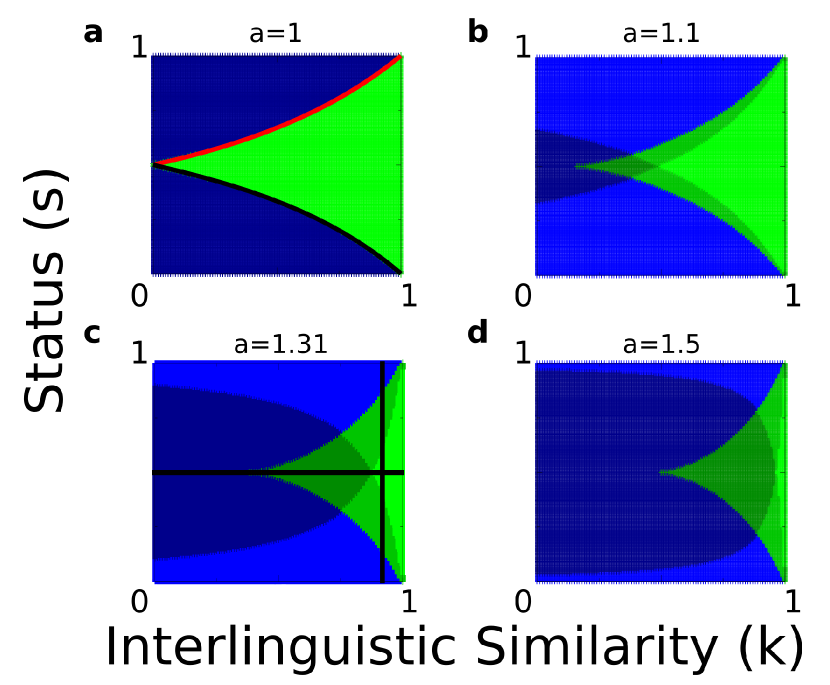
Figure 4: Regions of the $k-s$ space with different number of equilibrium points. a a=1: It is possible to compute analytically the curves $s_{P_{y}}(k_{P_{y}})$ (thick black line) and $s_{P_{x}}(k_{P_{x}})$ (thick red), which determine the frontiers above (below) which $P_{y}$ (respectively $P_{x}$) are unstable. The green area in which both $P_{y}$ and $P_{x}$ are unstable need the existence of an equilibrium point inside $A$ which is stable to attract the dynamics. The blue regions correspond to values of the parameters where either $P_{x}$ or $P_{y}$ are stable, but only one of them; meaning, in terms of competing languages, that one tongue must extinguish the other whatever the initial conditions. While the curves $s_{P_{y}}(k_{P_{y}})$ and $s_{P_{x}}(k_{P_{x}})$ were computed analytically, the colored regions were found out through computer simulations: a point of the $k-s$ space would be painted in blue if either of the attractors $P_{x}$ or $P_{y}$ were found after evolving the system a time large enough, and it would be painted in green whenever the simulations did not converge towards $P_{x}$ nor $P_{y}$ in a similar umber of iterations. Numerical and analytical results agree. b $a=1.1$, c $a=1.31$, d $a=1.5$: In either of these cases blue regions indicate that only the attractors $P_{x}$ and/or $P_{y}$ have been detected: both of them were detected in dark blue regions while only one of them was detected in lighter blue regions. Green regions indicate now that an attractor $P^{*}$ interior to $A$ has been detected: the darkest area correspond with $P^{*}$ being detected along $P_{x}$ and $P_{y}$ and the lighter areas means that one or two of $P_{x}$ and $P_{y}$ have not been detected. All these attractors were found numerically. The different shades of blue and green aim at demonstrating how the stability of the fixed points $P_{x}$ and $P_{y}$ depending upon $k$ and $s$ has been misread in previous studies of the model [25]. The outcome of the simulations are consistent with the analytical results, but they must be taken as strict approximations as long as they remain numerical conclusions. We found an interesting case in panel c that corresponds to $a=1.31$: the value previously used in the literature to fit real data. Thick black lines indicate the transversal sections along which bifurcation diagrams are taken in fig. 5.

The curves $s_{P_{x}}(k_{P_{x}})$ and $s_{P_{y}}(k_{P_{y}})$ are plotted in fig. 4a. There it is shown the stability of the different stable points for different values of $a$ in the $k-s$ space, but aided by computer simulations. We see that the numerical results match the analytical results for $s_{P_{x}}(k_{P_{x}})$ and $s_{P_{y}}(k_{P_{y}})$, and that these curves seem to evolve into the boundaries between different regimes as $a$ takes values larger than $1$.

For $a<1$ it is not possible to work out the stability of $P_{x}$ nor $P_{y}$ in a rigorous way. The Hessian matrix has diverging terms in this case: it is not well defined. We know, though, that there is always a third fixed point inside $A$ and computer simulations suggest that this interior equilibrium point is always stable for $a<1$. This would be in agreement with results obtained for the simpler precursor model [13] where a similar stable point is found for $a<1$ [20, 26].

4 Discussion and conclusions

The analytical results that we reached here are in partial discordance with those reported from previous numerical works [25]. Although the number of fixed points reckoned now could agree with previous accounts, the stability of them has been misread because of reasons that will be obvious right now. Notwithstanding this, the conclusions from [25] remain largely the same, as we will see. We first discuss the results for $a>1$ to compare directly with previous works and then we make some remarks about the cases $a\leq 1$.

In [25] the stability of the system was assessed through computer simulations only, thus stable fixed points were partly identified. Non-stable or saddle points did not stand out in these simulations because specific tests were not run therefore. It was concluded that one, two, or three stable equilibrium points existed in $A$, including the trivial ones at its boundary: $P_{x}$, $P_{y}$, and $P^{*}=(x^{*},y^{*})$; the later being the only equilibrium point explicitly detected in the interior of $A$. This matches exactly the picture drawn from the current work. The discrepancies arise regarding the stability of $P_{x}$ and $P_{y}$: The computational tools used in [25] yielded a result that strongly suggested that this stability depended upon $k$ and $s$ (dependence upon $a$ was not addressed: it was taken $a=1.31$ for historical reasons) and that $P^{*}$ was stable whenever it could be detected by simulations–as it could only be detected if it was an attractor of the dynamics in the discretized version of equations 2.

A plot was elaborated in [25] that divided the $k-s$ space of parameters in five regions that would correspond to five different stability/instability combinations of the equilibrium points. Namely: i) only $P_{x}$ or only $P_{y}$ is stable, $P^{*}$ is not detected; ii) both $P_{x}$ and $P_{y}$ are stable, $P^{*}$ is not detected; iii) the three possible points are detected and stable; iv) $P^{*}$ and either only $P_{x}$ or only $P_{y}$ are stable; and v) only $P^{*}$ is stable. In all five cases $P_{x}$ and $P_{y}$ were supposed to exist and to be instable whenever their basins of attraction were found empty by the computer simulations. An updated version of that plot is reproduced in fig. 4c with the same five regions colored with different shades of blue and green.

The interpretation given in [25] was not right although it was consistent with the numerical outcome. For example: we now know that $P_{x}$ and $P_{y}$ are always stable for $a>1$, disregarding the values of $k$ and $s$. We also know that at least one equilibrium point exists always in the interior of $A$, which may not be stable and which may lay in the boundary between the basins of attraction of $P_{x}$ and $P_{y}$. In fig. 1 they are shown the plots of the nullclines for the exact same parameters as those used in [25] and we readily see how for certain parameters some saddle points interior to $A$ approach $P_{x}$ or $P_{y}$ leading to a reduction of their basins of attraction. We now know that these equilibrium points never collapse into an unstable point. A basin of attraction may become undetectable to numerical means, and thus $P_{x}$ and $P_{y}$ may be deemed instable; but we have now found out analytically that $P_{x}$ and $P_{y}$ remain stable for any value of $k$ and $s$ if $a>1$. We were able to reproduce this numerical effect for the parameters used in [25] and for many others, as it can be seen in fig. 4b-d: lighter shades of blue or green indicate sets of parameters for which the computer simulations led to a wrong interpretation of the stability of some of the fixed points.

For $a>1$, the updated, more correct picture is as follows: There are always 2 stable trivial fixed points $P_{x}$ and $P_{y}$ and depending on the parameters $k$ and $s$ there are $1$, $2$, or $3$ more fixed points in the interior of $A$. It can be shown that if three points exist, one of them (termed $P^{*}$) must be stable. It can be argued that if there is only one fixed point inside $A$ it must be a saddle point; and that if there are three, those equilibrium points different from $P_{x}$, $P_{y}$, and $P^{*}$ must be saddle points as well. It can be guessed that the situation with $2$ equilibrium points inside $A$ corresponds to a saddle-node bifurcation as we transit through the $k-s$ space from a region with one to a region with three non-trivial fixed points. The existing analytical evidence and fig. 4, that shows the results of refined numerical simulations, are consistent with this view; although those facts that were not analytically proven in section 3 must be taken with enough care.

These equilibrium fixed points and their stability have got a direct interpretation for the phenomenon for which the model was developed in the first place: they determine whether two coexisting languages would remain alive together, or if one of them is going to take over and extinguish the other. Also, the nature of the fixed points reached by the dynamics determines whether individual bilingualism can be a stable trait. Given a pair of languages $X$ and $Y$ that coexist with status $s_{X}=s$ and $s_{Y}=1-s$ and interlinguistic similarity $k$ in a society with a fixed value of $a>1$, the model presents two well differentiated regions:

1. Coexistence is unstable: one language ends up suppressing the other and the bilingual group. What language survives depends on the initial distribution of speakers among monolinguals of each language and bilinguals. This case corresponds to only one equilibrium point– which turns out not to be stable–in the interior of $A$ and is depicted in figs. 1a-b. The regions in the $k-s$ space where this happens are colored in blue in fig. 4b-d.

2. Coexistence is possible depending on the parameters $k$, $s$, and $a$; and on the initial conditions of the dynamics. This case is the one with three stable equilibrium points $P_{x}$, $P_{y}$, and $P^{*}$. The initial conditions determine whether a language drives the other to extinction and makes bilingualism disappear, or if a steady state is reached ($P^{*}$) in which groups of monolingual speakers of both languages survive along with a bilingual group. This is what happens in figs. 1c-e; and parameters $k-s$ for which we find this situation are indicated in green in figs. 4b-d.

A third case regarding number of fixed points would exist at the boundary between these regions, but it does not seem to introduce any new behavior attending to the coexistence of languages. Coming back to the incomplete interpretation made of the results in [25], the two cases just outlined already include those configurations of parameters for which some attractors are so small that the extinction of a language or the coexistence of both of them is almost unavoidable without regard of the initial conditions; although we now know that this is never the case.

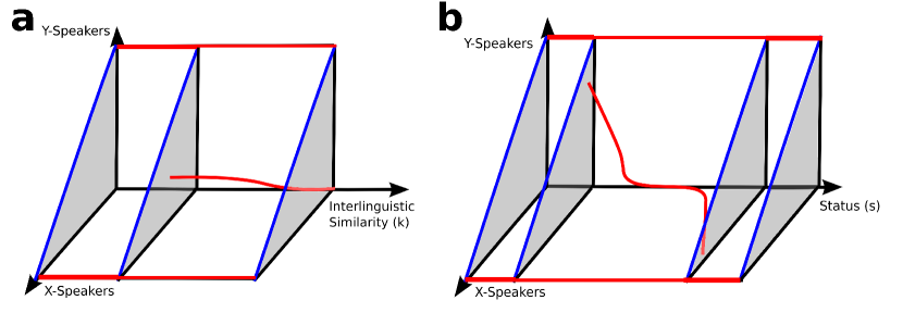
Figure 5: Bifurcation diagrams. Qualitative bifurcation diagrams are shown for fixed $a=1.31$ with: a varying $k$ and fixed $s=0.5$ and b varying $s$ and arbitrary $k$ close to $0.8$. Beginning with low $k$, when varying this parameter while holding $s$ fixed we depart from a situation in which $P_{x}$ and $P_{y}$ are stable and only one extra equilibrium point exists in the interior of $A$, a saddle point. Above a certain value of $k$ a new stable fixed point $P^{*}$ comes into existence. For varying $s$ and fixed $k$, if $k$ is large enough–as it is the case in this example–they exist two values of $s$ between which the third stable equilibrium $P^{*}$ point exists. The trajectory of $P^{*}$ through the $x-y$ space is qualitative in both cases.

We can see from the numerical simulations in fig. 4 that regions of the $k-s$ space where stable bilingualism is possible correspond to those with a more balanced status between languages. This balance is not so important for larger interlinguistic similarity: then a stable bilingual situation can be reached even for well distinct $s_{X}$ and $s_{Y}$, depending on the initial distribution of speakers. Further illustration of the role of $k$ and $s$ is made in fig. 5, that shows qualitative bifurcation diagrams of the stable fixed points when varying these parameters with fixed $a$.

The parameter $a$ was found relatively constant among cultures as indicated before [13], and this justified why it was not payed that much attention. But now we have also studied how the possible outcomes change as $a$ varies. First, considering only $a>1$, we see (fig. 4) that a larger $a$ means that the possibilities for stable bilingualism are reduced. This parameter was already considered in an analysis of the more basic Abrams-Strogatz model [17, 20, 26], and it was cleverly termed volatility parameter: the lower $a$ the more volatile a large group becomes and vice- versa. Thus, for larger $a$ bigger groups are more persistent and it is smaller the set of parameters for which it can be reached a more diluted distribution of speakers (this would be: a solution with speakers belonging to the bilingual groups, or communities with monolingual groups of each language coexisting together). For lower $a$, larger monolingual groups are not so permanent and a steady solution is easier to reach in which all languages coexist.

This volatility is a critical feature at $a=1$: $P_{x}$ and $P_{y}$ become unstable for some of the parameters $k$ and $s$ as it was said before. In terms of language dynamics this means that a monolingual group agglutinating all the speakers is no longer possible, whatever the initial conditions, if their statuses are close enough and depending on the similarity between languages. The region of the $k-s$ space where this happens can be seen in green in fig. 4a. In such cases the only stable solution in the long term is the coexistence of the monolingual groups along with the bilingual one. But still at $a=1$ one language might extinguish the other if its status is larger enough. There is a crucial difference between such an extinction and those happening for $a>1$: before, both languages could survive depending on the initial number of speakers of each one; now the extinction does not depend on this initial condition if the parameters are those needed for a language to take over (blue regions in fig. 4a).

The possibility of language extinction seems to change completely for $a<1$: then the volatility is so high that the monolingual options are never stable and the survival of both languages within their monolingual groups and along a bilingual group of speakers is guaranteed for any values of the parameters $k$ and $s$, and for any initial distribution of speakers. It was not possible to prove this very last result analytically beyond any doubt and it was obtained thanks to numerical simulations. This solution is consistent with similar outcomes for the seminal Abrams- Strogatz model [17, 20, 26], which should be the limit case for $k\rightarrow 0$ and $b\rightarrow 0$ of the equations under research in this paper.

4.1 Nature of the orbits and higher order contributions

A very important contribution of this paper is that brought in by lemma 3.2. It is clear its mathematical meaning: because of the nature of the field $(F_{x},F_{y})$ around a fixed point it is not possible to find closed–i.e. periodic–orbits. The same lemma also implies that any solution must consist of an exponential decay towards a fixed point: that an oscillatory decay is not possible. The interpretation of this result is rather strong when it comes down to languages: the extinction or raise of languages must be a monotonous phenomenon according to the present equations. Tendencies that could be expected, e.g. alternation in the preponderance of a language in a region, should not be observed. If such result were derived from real data, research should be focused on what is needed to complement the present model: “what would be the minimum elements that play a role in generating cyclic behavior in language competition?”, because those employed here would not suffice.

This lemma has got also some implications even if we would consider higher order or stochastic extensions of the present model. The equations investigated in this paper are nothing but a deterministic, mean field approach to a phenomenon that usually takes place on a stochastic environment. The next more realistic strategy to model language competition or coexistence departing from our current equations would be simulations of discrete agents that shift between the monolingual or the bilingual groups at random, being the transition probabilities given by equations 1. This is coherent if we suppose some free-will and variability to the speakers when deciding what language to use. We expect thus intrinsic stochasticity to be present and manifest throughout noise. The power spectrum of this noise can be investigated. The nature of the equilibrium points found for equations 2 establishes some important limitations to the kind of dynamics that can arise, as we will argue.

Several techniques are available in the literature to incorporate uncertainty in a deterministic model, from agent-based simulations with stochastic interaction events [29, 30] to theoretical considerations of a more analytical nature [31, 32, 33]. According to [34], we can determine that some interesting phenomena are ruled out from our model because of the lack of foci fixed points (again, recalling lemma 3.2). Namely, it is not possible to find Stochastic Amplification of Fluctuations (SAF), a phenomenon that offers a possible explanation to emergent quasi-oscillations observed in fields as diverse as ecology [33], epidemiology [35], or brain dynamics [34, 36]. In SAF the spectrum of the noise would present a prominent peak corresponding to these quasi-oscillations. Opposed to this, in our study case the power spectrum of intrinsic noise must present a monotonous decay proportional to $1/\omega^{2}$, and no outstanding peaks. We confirmed this result for many sets of parameters with agent-based simulations, as suggested above, finding no interesting features in the spectra, in agreement with the SAF theory.

SAF, if present, would be self evident in agent-based simulations. It could also be noted in series of real data if reports of language usage over time with enough precision were available. SAF is usually associated with adaptive reacting forces such as prey-predator or activator-repressor dynamics. Thus, reports of emergent oscillations in language dynamics could warn us ofthe presence of such forces driving language competition and serve for further, necessary refinement of the model. Numerical evidence shows that periodic solutions may appear if the status $s$ of the languages were allowed to change over time, which is a rather realistic extension of the model. Also, if there would exist models of language coexistence that presented SAF in a natural way, the observation (or the not observation) of this phenomenon in real data could help us determine which one is closer to reality.

References

- [1] J. Maynard-Smith, E. Szathmáry, The Major Transitions in Evolution, Oxford University Press, New York, 1997.
- [2] A. Wray, The Transition to Language, Oxford University Press, New York, 2002.
- [3] J.A. Hawkings, M. Gell-Mann, The Evolution of Human Languages, Addison-Wesley, Reading, Mass., 1992.
- [4] V. Loreto, L. Steels, Emergence of Language, Nature Phys. 3 (2007) 758.
- [5] I. Dyen, J.B. Kruskal, P. Black, An Indoeuropean classification: a lexicostatistical experiment, Trans. Am. Phil. Soc. 82 (1992) 3-132.
- [6] R. Axelrod, The dissemination of culture: A model with local convergence and global polarization, J. Conflict Resolut. 41 (1997) 203–226.
- [7] F. Petroni, M. Serva, Language distance and tree reconstruction, J. Stat. Mech. (2008) P08012.
- [8] C. Schulze, D. Stauffer, S. Wichmann, Birth, Survival and Death of Languages by Monte Carlo Simulation, Commun. Comput. Phys. 3 (2008) 271-294.
- [9] B. Corominas-Murtra, S. Valverde, R.V. Solé, The ontogeny of scale-free syntax networks: phase transitions in early language acquisition, Adv. Complex Syst. 12 (2009) 371-392.
- [10] R.V. Solé, B. Corominas-Murtra, S. Valverde, L. Steels, Language networks: their structure, function and evolution, Complexity 15(6) (2010) 20-26.
- [11] S. Nelson-Sathi, J.-M. List, H. Geisler, R.D. Gray, W. Martin, T. Dagan, Networks uncover hidden lexical borrowing in Indo-European language evolution, Proc. R. Soc. B 278 (2011) 1794–1803.
- [12] D.R. Amancio, O.N. Oliveira Jr., L.F. Costa, Using complex networks to quantify consistency in the use of words, J. Stat. Mech. (2012) P01004.
- [13] D.M. Abrams, S.H. Strogatz, Modelling the dynamics of language death, Nature 424 (2003) 900.
- [14] R.V. Solé, B. Corominas-Murtra, J. Fortuny, Diversity, competition, extinction: the ecophysics of language change, J. R. Soc. Interface 7 (2010) 1647–1664.
- [15] C. Castellano, S. Fortunato, V. Loreto, Statistical physics of social dynamics, Rev. Mod. Phys. 81 (2009) 591-646.
- [16] D. Stauffer, X. Castelló, V.M. Eguíluz, M. San Miguel, Microscopic Abrams–Strogatz model of language competition, Physica A 374(2) (2007) 835–842.
- [17] L. Chapel, X. Castelló, C. Bernard, G. Deffuant, V.M. Eguíluz, S. Martin, M. San Miguel, Viability and resilience of languages in competition, PLoS ONE 5 (2010) e8681.
- [18] M. Patriarca, T. Leppänen, Modeling language competition, Physica A 338(1–2) (2004) 296–299.
- [19] M. Patriarca, E. Heinsalu, Influence of geography on language competition, Physica A 388(2–3) (2009) 174–186.
- [20] F. Vázquez, X. Castelló, M. San Miguel, Agent based models of language competition: Macroscopic descriptions and order-disorder transitions, J. Stat. Mech. (2010) P04007.
- [21] W.S.-Y. Wang, J.W. Minett, The invasion of language: emergence, change and death, Trends Ecol. Evol. 20 (2005) 263-269.
- [22] X. Castelló, V.M. Eguíluz, M. San Miguel, Ordering dynamics with two non-excluding options: bilingualism in language competition, New J. Phys. 8 (2006) 308.
- [23] J. Mira, A. Paredes, Interlinguistic similarity and language death dynamics, Europhys. Lett. 69 (2005) 1031-1034.
- [24] J.W. Minett, W.S.-Y. Wang, Modeling endangered languages: The effects of bilingualism and social structure, Lingua 118 (2008) 19-45.
- [25] J. Mira, L.F. Seoane, J.J. Nieto, The importance of interlinguistic similarity and stable bilingualism when two languages compete, New J. of Phys. 13 (2011) 033007.
- [26] M. Patriarca, X. Castelló, J.R. Uriarte, V.M. Eguíluz, M. San Miguel, Modeling two-language competition dynamics, Adv. Complex Syst. 15(3-4) (2012) 1250048.
- [27] M.A. Nowak, N.L. Komarova, P. Niyogi, Computational and evolutionary aspects of language, Nature 417 (2002) 611-617.
- [28] Online supplementary material: http://www.youtube.com/watch?v=0IwkMjW_C8Q and http://www.usc.es/gl/departamentos/anmat/Green.html (this resource requires the Wolfram CDF player).
- [29] D.T. Gillespie, A General Method for Numerically Simulating the Stochastic Time Evolution of Coupled Chemical Reactions, J. Comput. Phys 2 (1976) 403-434.
- [30] D.T. Gillespie, Stochastic Simulation of Chemical Kinetics, Annu. Rev. Phys. Chem. 58 (2007) 35-55.
- [31] J.J. Nieto, R. Rodríguez-López, Analysis of a logistic differential model with uncertainty, I. J. Dynamical Systems and Differential Equations 1 (2008) 164-176.
- [32] R. Nisbet, W. Gurney, A simple mechanism for population cycles, Nature 263 (1976) 319-320.
- [33] A.J. McKane, T.J. Newman, Predator-prey cycles from resonant amplification of demographic stochasticity, Phys. Rev. Lett. 94 (2005) 218102.
- [34] J. Hidalgo, L.F. Seoane, J.M. Cortés, M.A. Muñoz, Stochastic Amplification of Fluctuations in Cortical Up-States, PLoS ONE 7(8) (2012) e40710.
- [35] D. Alonso, A.J. McKane, M. Pascual, Stochastic amplifications in epidemics. J. R. Soc. Interface 4 (2007) 575-578.
- [36] E. Wallace, M. Benayoun, W. van Drongelen, J. Cowan, Emergent Oscillations in Networks of Stochastic Spiking Neurons. PLoS ONE 6 (2011) e14804.