Performance of the stochastic MV-PURE estimator in highly noisy settings

Abstract

The stochastic MV-PURE estimator has been developed to provide linear estimation robust to ill-conditioning, high noise levels, and imperfections in model knowledge. In this paper, we investigate the theoretical performance of the stochastic MV-PURE estimator under varying level of additive noise. More precisely, we prove that the mean-square-error (MSE) of this estimator in the low signal-to-noise (SNR) region is much smaller than that obtained with its full-rank version, the minimum-variance distortionless estimator, and that the gap in performance is the larger the higher the noise level. These results shed light on the excellent performance of the stochastic MV-PURE estimator in highly noisy settings obtained in simulations so far. We extend here previously conducted numerical simulations to demonstrate a new insight provided by results of this paper in practical applications.

1 Introduction

The linear estimation of an unknown random vector of parameters in linear regression model has been a subject of a continuous research, amplified by widespread usage of the linear model $\textbf{y}=\textbf{H}\textbf{x}+\sqrt{\epsilon}\textbf{n}$ (e.g., in brain signal processing [1, 2] and wireless communications [3]), close link with array signal processing [4],[5, Sec.1.2], and low computational cost associated with linear estimation. In particular, the search for linear estimators more robust to ill-conditioning, high noise levels, and imperfections in model knowledge than the theoretically optimal [in the mean-square-error (MSE) sense] linear minimum-mean-squre-error (MMSE) estimator (Wiener filter) [6, 7] has long attracted researchers and practitioners attention, see e.g., [8, 9, 10, 11, 12] for an overview and recent solutions. One of the natural ways to increase robustness is to derive an estimator with carefully chosen additional constraints, resulting in an estimator which is theoretically suboptimal compared to the unconstrained solution, but achieves better performance in certain settings of interest (e.g., where only a finite sample estimate $\widehat{\textbf{H}}$ of a model matrix H is available in the linear model $\textbf{y}=\textbf{H}\textbf{x}+\sqrt{\epsilon}\textbf{n}$). An example of this approach is an estimator W minimizing MSE subject to the so-called distortionless constraint $\textbf{W}\textbf{H}=\textbf{I}$ which has been recently used as a robust solution for estimation of an unknown random vector [3, 13], and which is essentially equivalent to the celebrated best linear unbiased estimator (BLUE) [7] in deterministic estimation. Another provably robust technique is the reduced-rank approach [14, 15, 16, 17, 18, 19], very useful in ill-conditioned and highly noisy settings, as it introduces (usually a small amount of) bias in exchange for huge savings in variance, and in the adaptive case, it provides further benefit of usually lower computational load on the filtering process.

Thus, it would seem natural to extend the distortionless approach of the stochastic BLUE estimator to the reduced-rank case in order to achieve greater robustness to ill-conditioning, high noise levels, and imperfections in model knowledge. This has been achieved by introduction of the minimum-variance pseudo-unbiased reduced-rank estimation (MV-PURE) framework firstly proposed and solved in deterministic case in [20], and solved in the generalized formulation in deterministic case in [21], and extended to stochastic case in [22]. In this framework, the solution to an inverse problem of linear estimation of deterministic or random vector of parameters in linear regression model is derived as a rank-constrained solution of a hierarchical optimization problem, where, for a given rank constraint, the aim is to suppress bias (by simultaneous minimization of all unitarily invariant norms of an operator applied to the unknown parameter vector), and then to find among such estimators the one with minimum variance in deterministic case, and the one with minimum MSE in stochastic case.

However, in order to compare robustness properties of estimators considered, it is beneficient to compare their performances first in the theoretical case of perfect model knowledge. Then, aided with theoretical results serving as a benchmark, one would be able to determine the performance degradation of a given estimator (i.e., its robustness properties) in the presence of model uncertainties. Focusing on the stochastic MV-PURE estimator, we define conditions under which its rank reduction technique enables it in the theoretical settings of perfect model knowledge to achieve significantly lower MSE than its full-rank version, the stochastic BLUE estimator. The main result of this paper achieves this goal as it shows that the larger the power of additive noise, the larger the gap in performance between stochastic MV-PURE and stochastic BLUE estimators, and that the optimal rank is in fact monotonically decreasing with increasing noise level. These results indicate a common intuition that insistence on distortionless is an inadequate requirement in highly noisy conditions: the results of this paper derive conditions when this intuition is true. Furthermore, the results of this paper demonstrate clearly an interplay between noise levels and ill-conditioning of the model considered, which gives further insight into the scope of applicability of the stochastic MV-PURE estimator. We provide a numerical example, where we demonstrate a new insight and interpretation of the numerical simulations considered first in [22], where we employed the stochastic MV-PURE estimator as a linear receiver in a multiple-input multiple-output (MIMO) wireless communication system.

This paper expands results presented in part at conferences [23, 24].

2 Preliminaries

2.1 Stochastic linear model

In this paper we consider stochastic linear model of the form [6, 7]

$$\textbf{y}=\textbf{H}\textbf{x}+\sqrt{\epsilon}\textbf{n},$$ (1)

where $\textbf{y},\textbf{x},\textbf{n}$ represent observable random vector, random vector to be estimated, and additive noise, respectively, and where $\textbf{H}\in\mathbb{R}^{n\times m}$ is a known matrix of rank $m$, and $\epsilon>0$ is a known constant. We assume that x and n have zero mean and are uncorrelated, $\textbf{R}_{\textbf{x}\textbf{n}}=0$, and that $\textbf{R}_{\textbf{x}}\succ 0$ and $\textbf{R}_{\textbf{n}}\succ 0$ are known positive definite covariance matrices of x and n, respectively (by $\textbf{A}\succ 0$ we mean that matrix A is positive definite). From the previous assumption, $\textbf{R}_{\textbf{y}}=(\textbf{H}\textbf{R}_{\textbf{x}}\textbf{H}^{t}+\epsilon\textbf{R}_{\textbf{n}})\succ 0$ and $\textbf{R}_{\textbf{x}\textbf{y}}=\textbf{R}_{\textbf{x}}\textbf{H}^{t}$ are available and $rank(\textbf{R}_{\textbf{x}\textbf{y}})=m$. We define the norm of a random vector x by $\parallel\textbf{x}\parallel=\sqrt{tr\left[\mathrm{E}(\textbf{x}\textbf{x}^{t})\right]}=\sqrt{tr\left[\textbf{R}_{\textbf{x}}\right]}$ and we assume without loss of generality that $tr[\textbf{R}_{\textbf{n}}]=1$ so that $\parallel\sqrt{\epsilon}\textbf{n}\parallel^{2}=\epsilon.$

We consider the problem of linear estimation of x given y with the mean-square-error as the performance criterion. Thus, we seek to find a fixed matrix $\textbf{W}\in\mathbb{R}^{m\times n}$, called here an estimator, for which the estimate of x given by

$$\widehat{\textbf{x}}=\textbf{W}\textbf{y}$$ (2)

is optimal with respect to a certain criterion related to the mean-square-error (MSE) of $\widehat{\textbf{x}}$:

$$\mathrm{J}(\textbf{W})=\parallel\widehat{\textbf{x}}-\textbf{x}\parallel^{2}=tr[\textbf{W}\textbf{R}_{\textbf{y}}\textbf{W}^{t}]-2tr[\textbf{W}\textbf{R}_{\textbf{y}\textbf{x}}]+tr[\textbf{R}_{\textbf{x}}],$$ (3)

where as above $\textbf{R}_{\textbf{y}}$ and $\textbf{R}_{\textbf{x}}$ are the covariance matrices of y and x, respectively, and where $\textbf{R}_{\textbf{y}\textbf{x}}$ is the cross-covariance matrix between y and $\textbf{x}.$

2.2 MMSE, stochastic BLUE, and stochastic MV-PURE estimators

The unique solution to the problem of minimizing (3) is the linear minimum mean-square-error estimator (MMSE) $\textbf{W}_{MMSE}$, often called the Wiener filter, given by [6, 7]

$$\textbf{W}_{MMSE}=\textbf{R}_{\textbf{x}\textbf{y}}\textbf{R}_{\textbf{y}}^{-1}=\textbf{R}_{\textbf{x}}\textbf{H}^{t}(\textbf{H}\textbf{R}_{\textbf{x}}\textbf{H}^{t}+\epsilon\textbf{R}_{\textbf{n}})^{-1}.$$ (4)

However, as discussed in Section 1, the search for linear estimators under MSE criterion does not end here, certain solutions more robust to ill-conditioning, high noise levels, and imperfections in model knowledge need to be derived. The robustness of linear estimators having MSE (3) as the cost function can be greatly improved by adding constraints. An example of this approach is the stochastic BLUE estimator which is often called the distortionless MMSE estimator and has been widely employed in recent signal estimation and detection schemes [3, 13] and which is defined as a solution to the linearly restricted problem [7]:

$$\left\{\begin{array}[]{ll}\textrm{minimize}&\mathrm{J}(\textbf{W})\vspace{0.1cm}\\ \textrm{subject to}&\textbf{W}\textbf{H}=\textbf{I}_{m},\\ \end{array}\right.$$ (5)

with the unique solution

$$\textbf{W}_{BLUE}=(\textbf{H}^{t}\textbf{R}_{\textbf{y}}^{-1}\textbf{H})^{-1}\textbf{H}^{t}\textbf{R}_{\textbf{y}}^{-1}=(\textbf{H}^{t}\textbf{R}_{\textbf{n}}^{-1}\textbf{H})^{-1}\textbf{H}^{t}\textbf{R}_{\textbf{n}}^{-1}.$$ (6)

The stochastic MV-PURE estimator introduced in [22] is a reduced-rank extension of the approach (5), as it achieves the smallest distortion among all reduced-rank estimators. More precisely, the stochastic MV-PURE estimator is defined as a solution to the following problem for a given rank constraint $r\leq m$:

$$\left\{\begin{array}[]{ll}\textrm{minimize}&\mathrm{J}(\textbf{W}_{r})\\ \textrm{subject to}&\displaystyle\textbf{W}_{r}\in\bigcap_{\iota\in\mathfrak{I}}\mathcal{P}_{r}^{\iota},\\ \end{array}\right.$$ (7)

where

$$\mathcal{P}_{r}^{\iota}=\arg\min_{\textbf{W}_{r}\in\mathcal{X}_{r}^{m\times n}}\parallel\textbf{W}_{r}\textbf{H}-\textbf{I}_{m}\parallel_{\iota}^{2},\ \iota\in\mathfrak{I},$$ (8)

where $\mathcal{X}_{r}^{m\times n}:=\{\textbf{W}_{r}\in\mathbb{R}^{m\times n}:rank(\textbf{W}_{r})\leq r\leq m\}$ and where $\mathfrak{I}$ is the index set of all unitarily invariant norms. We recall here that a matrix norm $\iota$ is unitarily invariant if it satisfies $\parallel\textbf{U}\textbf{X}\textbf{V}\parallel_{\iota}=\parallel\textbf{X}\parallel_{\iota}$ for all orthogonal $\textbf{U}\in\mathbb{R}^{m\times m},\ \textbf{V}\in\mathbb{R}^{n\times n}$ and all $\textbf{X}\in\mathbb{R}^{m\times n}$ [25] [the Frobenius, spectral, and trace (nuclear) norm are examples of unitarily invariant norms]. The following Theorem provides a closed algebraic form of the stochastic MV-PURE estimator.

Theorem 1 ([22])

Consider the optimization problem (7). The following holds:

1. Assume that rank $r$ is constrained to $r<m$ and define the symmetric matrix K by

   $$\textbf{K}:=\left(\textbf{H}^{t}\textbf{R}_{\textbf{y}}^{-1}\textbf{H}\right)^{-1}-2\textbf{R}_{\textbf{x}}.$$ (9)

   Let the eigenvalue decomposition of the symmetric matrix K be given by $EVD(\textbf{K})=\textbf{E}\boldsymbol{\Delta}\textbf{E}^{t}$, with eigenvalues $\delta_{1}\leq\delta_{2}\leq\dots\leq\delta_{m}$ organized in nondecreasing order, and $e_{j}$ denotes the eigenvector associated with the eigenvalue $\delta_{j}$. Then the solution to problem (7), denoted by $\textbf{W}^{r}_{sMV-PURE}\in\mathbb{R}^{m\times n}$, is given by

   $$\textbf{W}^{r}_{sMV-PURE}=\textbf{E}_{r}\textbf{E}_{r}^{t}\textbf{W}_{BLUE},$$ (10)

   where $\textbf{W}_{BLUE}$ is defined in (6) and $\textbf{E}_{r}:=(e_{1},\ldots,e_{r}).$ If $\delta_{r}\neq\delta_{r+1}$, the solution is unique. Moreover, we have:

   $$\mathrm{J}(\textbf{W}^{r}_{sMV-PURE})=\sum_{i=1}^{r}\delta_{i}+tr[\textbf{R}_{\textbf{x}}].$$ (11)

2. If no rank constraint is imposed, i.e., when $r=m$, then the solution to problem (7) is uniquely given by $\textbf{W}^{m}_{sMV-PURE}=\textbf{W}_{BLUE}$. In particular, we have:

   $$\mathrm{J}(\textbf{W}^{m}_{sMV-PURE})=\mathrm{J}(\textbf{W}_{BLUE})=\sum_{i=1}^{m}\delta_{i}+tr[\textbf{R}_{\textbf{x}}].$$ (12)

The following Remark follows directly from Theorem 1 and will be useful later on.

Remark 1

Let us set rank constraint $r<m.$ We have

$$\mathrm{J}(\textbf{W}_{sMV-PURE}^{r})<\mathrm{J}(\textbf{W}_{sMV-PURE}^{r+1})<$$

$$\dots<\mathrm{J}(\textbf{W}_{sMV-PURE}^{m})=\mathrm{J}(\textbf{W}_{BLUE})\Longleftrightarrow\delta_{r+1}>0.$$ (13)

In particular, the optimal rank $r_{opt}$ of the stochastic MV-PURE estimator, for which $\mathrm{J}(\textbf{W}_{sMV-PURE}^{r_{opt}})$ is the smallest, is such that

$$r_{opt}=\max\left\{s\in\{1,2,\ldots,m\}\mid\delta_{s}<0\right\}.\ \square$$ (14)

2.3 Variational characterization of eigenvalues of symmetric matrices

The following theorem due to Weyl shows how eigenvalues of $A+B$ compare to eigenvalues of $A$, where $A,B\in\mathbb{R}^{m\times m}$ are symmetric matrices. This result will play an important role in derivation of the results of Section 3.

Fact 1 (Weyl [25, p.181])

Let $A,B\in\mathbb{R}^{m\times m}$ be symmetric matrices, and let the eigenvalues $\lambda_{i}(A)$, $\lambda_{i}(B)$, and $\lambda_{i}(A+B)$ be organized in nondecreasing order. For each $k=1,2,\dots,m$ we have:

$$\lambda_{k}(A)+\lambda_{1}(B)\leq\lambda_{k}(A+B)\leq\lambda_{k}(A)+\lambda_{m}(B).$$ (15)

3 Performance analysis under varying levels of signal-to-noise
ratio

We note first the following Lemma which gives us an alternative expression of matrix K defined in (9). It will be used below to prove the main results of this paper.

Lemma 1

With notation as in model (1), the following equality holds:

$$(\textbf{H}^{t}\textbf{R}_{\textbf{y}}^{-1}\textbf{H})^{-1}=\epsilon(\textbf{H}^{t}\textbf{R}_{\textbf{n}}^{-1}\textbf{H})^{-1}+\textbf{R}_{\textbf{x}},$$ (16)

and thus K (9) in Theorem 1 can be expressed as:

$$\textbf{K}=\left(\textbf{H}^{t}\textbf{R}_{\textbf{y}}^{-1}\textbf{H}\right)^{-1}-2\textbf{R}_{\textbf{x}}=\epsilon\left(\textbf{H}^{t}\textbf{R}_{\textbf{n}}^{-1}\textbf{H}\right)^{-1}-\textbf{R}_{\textbf{x}}.$$ (17)

Proof: Let us recall that in model (1) we have $\textbf{R}_{\textbf{x}\textbf{y}}=\textbf{R}_{\textbf{x}}\textbf{H}^{t}$ (and therefore $\textbf{R}_{\textbf{y}\textbf{x}}=\textbf{H}\textbf{R}_{\textbf{x}}$), and consider the covariance matrix

$$\textbf{E}\left[(\textbf{W}\textbf{y}-\textbf{x})(\textbf{W}\textbf{y}-\textbf{x})^{t}\right]=\textbf{W}\textbf{R}_{\textbf{y}}\textbf{W}^{t}-\textbf{W}\textbf{H}\textbf{R}_{\textbf{x}}-\textbf{R}_{\textbf{x}}\textbf{H}^{t}\textbf{W}^{t}+\textbf{R}_{\textbf{x}}.$$ (18)

By inserting the first expression of $\textbf{W}_{BLUE}=(\textbf{H}^{t}\textbf{R}_{\textbf{y}}^{-1}\textbf{H})^{-1}\textbf{H}^{t}\textbf{R}_{\textbf{y}}^{-1}$ (6) into (18) we obtain $\textbf{E}\left[(\textbf{W}_{BLUE}\textbf{y}-\textbf{x})(\textbf{W}_{BLUE}\textbf{y}-\textbf{x})^{t}\right]=(\textbf{H}^{t}\textbf{R}_{\textbf{y}}^{-1}\textbf{H})^{-1}-\textbf{R}_{\textbf{x}}.$ However, since $\textbf{R}_{\textbf{y}}=\textbf{H}\textbf{R}_{\textbf{x}}\textbf{H}^{t}+\epsilon\textbf{R}_{\textbf{n}}$, from the second expression of $\textbf{W}_{BLUE}=(\textbf{H}^{t}\textbf{R}_{\textbf{n}}^{-1}\textbf{H})^{-1}\textbf{H}^{t}\textbf{R}_{\textbf{n}}^{-1}$ (6) we obtain from (18) also the alternative expression $\textbf{E}\left[(\textbf{W}_{BLUE}\textbf{y}-\textbf{x})(\textbf{W}_{BLUE}\textbf{y}-\textbf{x})^{t}\right]=\epsilon(\textbf{H}^{t}\textbf{R}_{\textbf{n}}^{-1}\textbf{H})^{-1}.$ $\ \square$

The following Theorem demonstrates the usefulness of the reduced-rank approach of the stochastic MV-PURE estimator in highly noisy settings.

Theorem 2

Let $EVD(\textbf{H}^{t}\textbf{R}_{\textbf{n}}^{-1}\textbf{H})=\textbf{M}\boldsymbol{\Upsilon}\textbf{M}^{t}$ be an eigenvalue decomposition of

$$\textbf{H}^{t}\textbf{R}_{\textbf{n}}^{-1}\textbf{H}\succ 0,$$ (19)

with eigenvalues $\upsilon_{1}\geq\upsilon_{2}\geq\dots\geq\upsilon_{m}>0.$ Moreover, let $EVD(\textbf{R}_{\textbf{x}})=\textbf{N}\boldsymbol{\Gamma}\textbf{N}^{t}$ be an eigenvalue decomposition of $\textbf{R}_{\textbf{x}}\succ 0$ with eigenvalues $\gamma_{1}\geq\gamma_{2}\geq\dots\geq\gamma_{m}>0.$ Then, for each rank constraint $r<m$, if the power of additive noise $\epsilon$ is such that:

$$\epsilon>\upsilon_{r+1}\gamma_{1}$$ (20)

then:

$$\mathrm{J}(\textbf{W}_{sMV-PURE}^{r})<\mathrm{J}(\textbf{W}_{sMV-PURE}^{r+1})<$$

$$\dots<\mathrm{J}(\textbf{W}_{sMV-PURE}^{m})=\mathrm{J}(\textbf{W}_{BLUE}).$$ (21)

In particular, relation between (20) and (2) guarantees that the reduced-rank approach of the stochastic MV-PURE estimator enables it to achieve lower mean-square-error than of the stochastic BLUE estimator for all $\epsilon>\upsilon_{m}\gamma_{1}.$ Moreover, if:

$$\upsilon_{r}\gamma_{m}>\epsilon>\upsilon_{r+1}\gamma_{1}$$ (22)

then $r=r_{opt}=\max\left\{s\in\{1,2,\ldots,m\}\mid\delta_{s}<0\right\}.$

Proof: From our assumptions, we have $EVD[(\textbf{H}^{t}\textbf{R}_{\textbf{n}}^{-1}\textbf{H})^{-1}]=\textbf{M}\boldsymbol{\Upsilon}^{-1}\textbf{M}^{t}$ with eigenvalues $0<\upsilon_{1}^{-1}\leq\upsilon_{2}^{-1}\leq\dots\leq\upsilon_{m}^{-1}$, and $EVD(-\textbf{R}_{\textbf{x}})=\textbf{N}(-\boldsymbol{\Gamma})\textbf{N}^{t}$ with eigenvalues $-\gamma_{1}\leq-\gamma_{2}\leq\dots\leq-\gamma_{m}<0.$ Thus, if we denote an eigenvalue decomposition of $\textbf{K}=\epsilon\left(\textbf{H}^{t}\textbf{R}_{\textbf{n}}^{-1}\textbf{H}\right)^{-1}-\textbf{R}_{\textbf{x}}$ (17) by $EVD(\textbf{K})=\textbf{E}\boldsymbol{\Delta}\textbf{E}^{t}$, with eigenvalues $\delta_{1}\leq\delta_{2}\leq\dots\leq\delta_{m}$ organized in nondecreasing order, from Fact 1 in Section 2.3, upon setting $\textbf{A}=\epsilon(\textbf{H}^{t}\textbf{R}_{\textbf{n}}^{-1}\textbf{H})^{-1}$ and $\textbf{B}=-\textbf{R}_{\textbf{x}}$, we obtain for each $s=1,2,\dots,m$

$$\epsilon\upsilon_{s}^{-1}-\gamma_{1}\leq\delta_{s}\leq\epsilon\upsilon_{s}^{-1}-\gamma_{m}.$$ (23)

Therefore, from the first inequality above it is seen that condition (20) ensures $\delta_{r+1}>0$, which in view of (1) is equivalent to (2). Similarly, if $\epsilon$ satisfies the more stringent condition (22), then not only $\delta_{r+1}>0$, but also $\delta_{r}<0$, which in view of (14) implies that $\displaystyle r=r_{opt}.$ $\ \square$

We note that Theorem 2 provides an insight into an interplay between ill-conditioning of $\textbf{H}^{t}\textbf{R}_{\textbf{n}}^{-1}\textbf{H}$ and noise power $\epsilon.$ Namely, for fixed $\textbf{R}_{\textbf{x}}\succ 0$, if $\textbf{H}^{t}\textbf{R}_{\textbf{n}}^{-1}\textbf{H}$ has a large condition number defined as the ratio of the largest eigenvalue to the smallest, e.g., if it possesses some vanishingly small trailing eigenvalues, then in such settings it suffices for the noise power $\epsilon$ to be relatively very small for the reduced-rank approach to be useful, in the sense of relation given by (20)-(2).

It should be also noted that Theorem 2 can be easily generalized, e.g., by simply swapping the roles of A and B in the Proof of Theorem 2, which would give (in virtue of Fact 1 in Section 2.3) pairs of bounds on the eigenvalues of K, alternative to those stated in (23). Indeed, many different alternatives to the bounds presented in (23) can be obtained by applying the more general Theorem 4.3.7 in [25, pp.184-185], of which Fact 1 in Section 2.3 is a special case. Nevertheless, bounds (23) used in the Proof of Theorem 2 give in our opinion naturally interpretable conditions (20) and (22).

However, conditions (22) do not guarantee that the optimal rank of the stochastic MV-PURE estimator is the lower the larger the power $\epsilon$ of additive noise, for the general case of a not necessarily white input vector x. This goal is achieved in the following Theorem.

Theorem 3

For fixed $\textbf{R}_{\textbf{x}}\succ 0$ and $\textbf{R}_{\textbf{n}}\succ 0$ in the stochastic linear model in Sec.2.1, the optimal rank of the stochastic MV-PURE estimator (for which it achieves the smallest MSE among all rank constraints) is monotonically decreasing with increasing power $\epsilon$ of the additive noise.

Proof: Let us denote first an eigenvalue decomposition of matrix $\textbf{K}=\epsilon\left(\textbf{H}^{t}\textbf{R}_{\textbf{n}}^{-1}\textbf{H}\right)^{-1}-\textbf{R}_{\textbf{x}}$ (17) by $EVD(\textbf{K})=\textbf{E}\boldsymbol{\Delta}\textbf{E}^{t}$, with eigenvalues $\delta_{1}\leq\delta_{2}\leq\dots\leq\delta_{m}$ organized in nondecreasing order. We recall from Remark 1 that a rank constraint $r_{opt}$ is optimal in our sense if it satisfies

$$r_{opt}=\max\left\{s\in\{1,2,\ldots,m\}\mid\delta_{s}<0\right\}.$$

We will show now that all eigenvalues of K grow monotonically with increasing $\epsilon$ which is a sufficient condition for the claim in the Theorem since in such a case $r_{opt}$ can only be monotonically decreasing with increasing $\epsilon.$

To this end, denote by $\lambda_{k}(\textbf{X})$ the eigenvalues of a given symmetric matrix X organized in nondecreasing order and consider $\epsilon_{1}>\epsilon_{0}>0$ so that

$$\epsilon_{1}(\textbf{H}^{t}\textbf{R}_{\textbf{n}}^{-1}\textbf{H})^{-1}-\textbf{R}_{\textbf{x}}=\textbf{A}+\textbf{B},$$ (24)

where $\textbf{A}=\epsilon_{0}(\textbf{H}^{t}\textbf{R}_{\textbf{n}}^{-1}\textbf{H})^{-1}-\textbf{R}_{\textbf{x}}$ and $\textbf{B}=\epsilon_{2}(\textbf{H}^{t}\textbf{R}_{\textbf{n}}^{-1}\textbf{H})^{-1}$ with $\epsilon_{2}=\epsilon_{1}-\epsilon_{0}>0.$ Note that B so defined is a positive definite matrix, thus all eigenvalues of B are strictly positive. Hence, from the first inequality in Fact 1 in Section 2.3 we obtain that

$$\forall k=1,\dots,m\quad\lambda_{k}\left[\epsilon_{1}(\textbf{H}^{t}\textbf{R}_{\textbf{n}}^{-1}\textbf{H})^{-1}-\textbf{R}_{\textbf{x}}\right]\geq\lambda_{k}\left[\epsilon_{0}(\textbf{H}^{t}\textbf{R}_{\textbf{n}}^{-1}\textbf{H})^{-1}-\textbf{R}_{\textbf{x}}\right]+$$

$$\lambda_{1}\left[\epsilon_{2}(\textbf{H}^{t}\textbf{R}_{\textbf{n}}^{-1}\textbf{H})^{-1}\right]>\lambda_{k}\left[\epsilon_{0}(\textbf{H}^{t}\textbf{R}_{\textbf{n}}^{-1}\textbf{H})^{-1}-\textbf{R}_{\textbf{x}}\right],\quad$$ (25)

which completes the proof. $\ \square$

4 Numerical example

In digital signal processing applications, the following setup is frequently considered:

$$\textbf{y}_{c}=\textbf{H}_{c}\textbf{x}_{c}+\sqrt{\epsilon}\textbf{n}_{c},$$ (26)

where $\textbf{H}_{c}\in\mathbb{C}^{N\times M}$ is a complex Gaussian channel between input signal $\textbf{x}_{c}\in\mathbb{C}^{M}$ and output signal $\textbf{y}_{c}\in\mathbb{C}^{N}$ corrupted by additive Gaussian noise $\textbf{n}_{c}\in\mathbb{C}^{N}.$ Then, the task is to estimate linearly $\textbf{x}_{c}$ by $\widehat{\textbf{x}}_{c}=\textbf{W}\textbf{y}_{c}$ under MSE criterion.

We set $N=M=8$ and assume zero-mean temporally white circular Gaussian noise random vector with spatial covariance matrix $\textbf{R}_{\textbf{n}_{c}}\succ 0$, where the entries of $\textbf{H}_{c}$ are zero-mean i.i.d. Gaussian random variables of unity variance, and where input signal $\textbf{x}_{c}$ is independent from noise (thus $\textbf{R}{\textbf{x}_{c}\textbf{n}_{c}}=0\in\mathbb{R}^{M\times N}$) and consists of symbols drawn uniformly and independently from QPSK=$\{1+i,1-i,-1+i,-1-i\}$ constellation. We define signal-to-noise ratio (SNR) as:

$$\textrm{SNR}={{\sigma^{2}_{h}}\over{\epsilon tr[R_{\textbf{n}_{c}}]}}={{1}\over{\epsilon}},$$ (27)

where $\sigma^{2}_{h}=1$ is the variance of the elements of $\textbf{H}_{c}$ and where we assume without loss of generality that $tr[\textbf{R}_{\textbf{n}_{c}}]=1.$ The noise covariance matrix $\textbf{R}_{\textbf{n}_{c}}$ is the same throughout the remainder of Section 4, and we assume below that $Q=200$ data blocks have been transmitted.

In [22], the effectiveness of the stochastic MV-PURE estimator was demonstrated in a scenario of a multiple-input multiple-output (MIMO) wireless communication systems. However, it was unclear how the power of the additive noise and ill-conditioning of the model considered affect performance of the stochastic MV-PURE estimator, especially compared to its full-rank version, the stochastic BLUE estimator. Thanks to the results of Section 3, we can answer these questions below.

To this end, let us first cast the complex model (26) into its equivalent real-valued representation:

$$\textbf{y}=\left(\begin{array}[]{c}Re({\textbf{y}_{c}})\\ Im({\textbf{y}_{c}})\\ \end{array}\right)\!\!,\ \textbf{n}=\left(\begin{array}[]{c}Re({\textbf{n}_{c}})\\ Im({\textbf{n}_{c}})\\ \end{array}\right)\!\!,\ \textbf{x}=\left(\begin{array}[]{c}Re({\textbf{x}_{c}})\\ Im({\textbf{x}_{c}})\\ \end{array}\right)\!\!,$$ (28)

and:

$$\textbf{H}=\left(\begin{array}[]{cc}Re({\textbf{H}_{c}})&-Im({\textbf{H}_{c}})\\ Im({\textbf{H}_{c}})&Re({\textbf{H}_{c}})\\ \end{array}\right)\!\!,\ \textbf{R}_{\textbf{n}}=1/2\left(\begin{array}[]{cc}R_{\textbf{n}_{c}}&0\\ 0&R_{\textbf{n}_{c}}\\ \end{array}\right)\!\!,$$ (29)

with $\textbf{R}_{\textbf{x}}=\textbf{I}_{16}.$ Then, the sample mean estimate of the mean-square-error (3) is given by:

$$\widehat{\mathrm{J}(\textbf{W})}={{1}\over{Q}}\sum_{q=1}^{Q}\parallel\widehat{\textbf{x}}_{c_{q}}-\textbf{x}_{c_{q}}\parallel^{2},$$ (30)

where $Q$ is the number of data blocks, and $\widehat{\textbf{x}}_{c_{q}}$ is an estimate of $\textbf{x}_{c_{q}}$ obtained from its real-valued representation $\widehat{\textbf{x}}_{q}=\textbf{W}\textbf{y}_{q}$ as $\widehat{\textbf{x}}_{c_{q}}=[\textbf{I}_{8}\quad i\textbf{I}_{8}]\widehat{\textbf{x}}_{q}.$ In figures below, we represent the sample mean-square-error (30) in decibels [$10\log_{10}\widehat{\mathrm{J}(\textbf{W})}$] as $MSE[dB]$. Furthermore, we consider below levels of

$$SNR[dB]=(-4,-2,0,2,4,6,8)$$

which corresponds to $\epsilon$ values of

$$\epsilon=(2.51,1.58,1,0.63,0.4,0.25,0.16),$$ (31)

respectively, cf. (27).

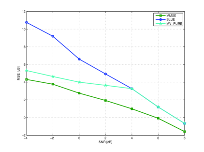
Figure 1: MSE [dB] vs. SNR [dB] for sample channel realization in theoretical case.

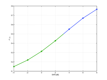
Figure 2: Monotonical decrease of $\sigma_{15}$ with decreasing $SNR[dB]$ in theoretical case. The 0.5 threshold is crossed between $SNR[dB]=2$ and $SNR[dB]=4.$

In the theoretical case of exact model knowledge, we present in Fig.1 a performance comparison for sample realization of channel $\textbf{H}_{c}$, where the eigenvalues of $\textbf{H}^{t}\textbf{R}_{\textbf{n}}^{-1}\textbf{H}$ are found to be:

$$(\upsilon_{1}=14102,\upsilon_{2}=14102,\upsilon_{3}=550,\upsilon_{4}=550,\dots,\\ \upsilon_{13}=5.1,\upsilon_{14}=5.1,\upsilon_{15}=0.43,\upsilon_{16}=0.43).$$ (32)

We note that eigenvalues of $\textbf{H}^{t}\textbf{R}_{\textbf{n}}^{-1}\textbf{H}$ come in pairs in virtue of the real-valued representation via (28)-(29). Therefore, using Theorem 2 for $\textbf{R}_{\textbf{x}}=\textbf{I}_{16}$ (thus $\gamma_{i}=1$ for $i=1,\dots,16$ in Theorem 2) from (31) and (32) we obtain that $r_{opt}=14$ for $SNR[dB]=(-4,-2,0,2)$ and $r_{opt}=16$ for $SNR[dB]=(4,6,8)$, for channel realization as in Fig.1. It is also seen that even a relatively mild ill-conditioning of $\textbf{H}^{t}\textbf{R}_{\textbf{n}}^{-1}\textbf{H}$ embodied in the last two trailing eigenvalues indicates that rank-reduction yields improved performance also for higher values of $SNR[dB]$, cf. also comments below Theorem 2.

Moreover, from Theorem 1 and Remark 1 it is simple to verify that for $\textbf{R}_{\textbf{x}}=\textbf{I}_{16}$ one has from (14) that

$$r_{opt}=\max\left\{s\in\{1,2,\ldots,m\}\mid\sigma_{s}>0.5\right\},$$ (33)

where $\sigma_{1}\geq\sigma_{2}\geq\dots\geq\sigma_{16}>0$ are the eigenvalues of $\textbf{H}^{t}\textbf{R}_{\textbf{y}}^{-1}\textbf{H}.$ Thus, from Theorem 3 we conclude that if we find $\sigma_{14}>0.5$ and $\sigma_{15}<0.5$ for certain $SNR[dB]$ levels $x,y\in\{-4,-2,0,2,4,6,8\}$ with $y<x$, then one can set $r_{opt}=14$ without any numerical simulations for all levels of $SNR[dB]$ such that

$$y\leq SNR[dB]\leq x.$$

In particular, the value of $\sigma_{15}$ must be monotonically decreasing with decreasing levels of $SNR[dB]$, as demonstrated in Fig.2. This can be deducted from the proof of Theorem 3 which shows that all eigenvalues of $\textbf{K}=\left(\textbf{H}^{t}\textbf{R}_{\textbf{y}}^{-1}\textbf{H}\right)^{-1}-2\textbf{R}_{\textbf{x}}$ (which may be expressed here as $\sigma_{1}^{-1}-2\leq\sigma_{2}^{-1}-2\leq\dots\leq\sigma_{16}^{-1}-2$) grow monotonically with decreasing levels of $SNR[dB].$

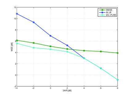
Figure 3: MSE [dB] vs. SNR [dB] for sample channel realization in practical case.

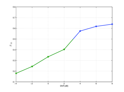
Figure 4: Monotonical decrease of $\widetilde{\sigma}_{15}$ with decreasing $SNR[dB]$ in practical case. The 0.5 threshold is crossed between $SNR[dB]=2$ and $SNR[dB]=4.$

We consider now the case where the channel matrix $\textbf{H}_{c}$ is assumed to be known at the receiver with error such that $\widetilde{\textbf{H}}_{c}=\textbf{H}_{c}+\textbf{E}_{c}$, where the entries of the error matrix $\textbf{E}_{c}$ are i.i.d. drawn from Gaussian distribution with zero-mean and variance $10^{-4}$. Moreover, for the results presented below we assume that neither the noise covariance matrix $R_{\textbf{n}_{c}}$ nor the noise power $\epsilon$ are available at the receiver side, and we only use the sample estimate of the covariance matrix of observed data $\textbf{R}_{\textbf{y}}$:

$$\widehat{\textbf{R}_{\textbf{y}}}={{1}\over{Q}}\sum_{q=1}^{Q}\textbf{y}_{q}\textbf{y}_{q}^{t},$$ (34)

where $Q=200$ is the number of data blocks available. In Fig.3-4 we use the perturbed version of the channel matrix $\textbf{H}_{c}$ used in Fig.1-2, and the same data block transmitted, to clearly illustrate the difference between results obtained under complete and incomplete model knowledge.

In current settings one cannot use Theorem 2 directly due to unknown $\textbf{R}_{\textbf{n}}$ and $\epsilon.$ However, we may estimate the last two trailing eigenvalues $\sigma_{15},\sigma_{16}$ of $\textbf{H}^{t}\textbf{R}_{\textbf{y}}^{-1}\textbf{H}$ via the last two trailing eigenvalues $\widetilde{\sigma}_{15},\widetilde{\sigma}_{16}$ of $\widetilde{\textbf{H}}^{t}\widehat{\textbf{R}_{\textbf{y}}}^{-1}\widetilde{\textbf{H}}$, and similarly as in Fig.2 we shall utilize Theorem 3 to set $r=14$ for $SNR[dB]=(-4,-2,0,2)$ and $r=16$ for $SNR[dB]=(4,6,8).$ The results are presented in Fig.3-4, where in Fig.3 it is seen that the ranks selected remain correct in the current settings, as the trailing eigenvalues of $\textbf{H}^{t}\textbf{R}_{\textbf{y}}^{-1}\textbf{H}$ are not significantly perturbed in $\widetilde{\textbf{H}}^{t}\widehat{\textbf{R}_{\textbf{y}}}^{-1}\widetilde{\textbf{H}}$, which is demonstrated in Fig.4.

Finally, we would like to note that the mildly ill-conditioned matrix $\textbf{H}^{t}\textbf{R}_{\textbf{n}}^{-1}\textbf{H}$ used in simulations above implied that the rank-reduction capability of the stochastic MV-PURE estimator provided gain in performance over the stochastic BLUE estimator in just over half of the $SNR[dB]$ values considered, which allowed us to demonstrate transparently the main results of this paper. However, the averaged performance (over 10 000 Monte-Carlo runs) demonstrated in [22] showed that the stochastic BLUE estimator is on average more severely penalized by ill-conditioning of $\textbf{H}^{t}\textbf{R}_{\textbf{n}}^{-1}\textbf{H}$ than in a delicately ill-conditioned settings considered in this section.

5 Concluding remarks

In the low SNR regime, we proved that the stochastic MV-PURE estimator achieves drastic improvement in performance over its full-rank version, the stochastic BLUE estimator. This result demonstrates that many of the existing applications of the stochastic BLUE estimator may benefit by employing instead the reduced-rank approach of the stochastic MV-PURE estimator in highly noisy conditions.

References

- Cichocki and Amari [2002] A. Cichocki, S.-I. Amari, Adaptive Blind Signal and Image Processing: Learning Algorithms and Applications, John Wiley & Sons, New York, 2002.
- Piotrowski et al. [2013] T. Piotrowski, C. Zaragoza-Martinez, D. Gutierrez, I. Yamada, MV-PURE estimator of dipole source signals in EEG, in: Proc. ICASSP, Vancouver, Canada, May 2013. To appear.
- Wang and Poor [2004] X. Wang, H. V. Poor, Wireless Communication Systems, Prentice Hall, Upper Saddle River, 2004.
- Van Trees [2002] H. L. Van Trees, Optimum Array Processing, John Wiley & Sons, New York, 2002.
- Pezeshki et al. [2010] A. Pezeshki, L. L. Scharf, E. K. P. Chong, The geometry of linearly and quadratically constrained optimization problems for signal processing and communications, Journal of The Franklin Institute 347 (2010) 818–835.
- Luenberger [1969] D. G. Luenberger, Optimization by Vector Space Methods, John Wiley & Sons, New York, 1969.
- Kailath et al. [2000] T. Kailath, A. H. Sayed, B. Hassibi, Linear Estimation, Prentice Hall, New Jersey, 2000.
- Huber [1964] P. J. Huber, Robust estimation of a location parameter, The Annals of Mathematical Statistics 35 (1964) 73–101.
- Kassam and Poor [1985] S. A. Kassam, H. V. Poor, Robust techniques for signal processing: a survey, Proc. IEEE 73 (1985) 433–481.
- Eldar and Merhav [2004] Y. C. Eldar, N. Merhav, A competitive minimax approach to robust estimation of random parameters, IEEE Trans. Signal Processing 52 (2004) 1931–1946.
- Eldar and Merhav [2005] Y. C. Eldar, N. Merhav, Minimax MSE-ratio estimation with signal covariance uncertainties, IEEE Trans. Signal Processing 53 (2005) 1335–1347.
- Rong et al. [2005] Y. Rong, S. Shahbazpanahi, A. B. Gershman, Robust linear receivers for space-time block coded multiaccess MIMO systems with imperfect channel state information, IEEE Trans. Signal Processing 53 (2005) 3081–3090.
- Shahbazpanahi et al. [2004] S. Shahbazpanahi, M. Beheshti, A. B. Gershman, M. Gharavi-Alkhansari, K. M. Wong, Minimum-variance linear receivers for multiaccess MIMO wireless systems with space-time block coding, IEEE Trans. Signal Processing 52 (2004) 3306–3313.
- Brillinger [1975] D. R. Brillinger, Time Series: Data Analysis and Theory, Holt, Rinehart and Winston, New York, 1975.
- Scharf [1991] L. L. Scharf, The SVD and reduced rank signal processing, Signal Processing 25 (1991) 113–133.
- Stoica and Viberg [1996] P. Stoica, M. Viberg, Maximum likelihood parameter and rank estimation in reduced-rank multivariate linear regressions, IEEE Trans. Signal Processing 44 (1996) 3069–3078.
- Scharf and Thomas [1998] L. L. Scharf, J. K. Thomas, Wiener filters in canonical coordinates for transform coding, filtering, and quantizing, IEEE Trans. Signal Processing 46 (1998) 647–654.
- de Lamare et al. [2012] R. C. de Lamare, L. Wang, R. Fa, Adaptive reduced-rank LCMV beamforming algorithms based on joint iterative optimization of filters: Design and analysis, Signal Processing 90 (2012) 640–652.
- Huang et al. [2012] F. Huang, W. Sheng, C. Lu, X. Ma, A fast adaptive reduced rank transformation for minimum variance beamforming, Signal Processing 92 (2012) 2881–2887.
- Yamada and Elbadraoui [2006] I. Yamada, J. Elbadraoui, Minimum-variance pseudo-unbiased low-rank estimator for ill-conditioned inverse problems, in: Proc. ICASSP, Toulouse, France, May 2006, pp. 325–328.
- Piotrowski and Yamada [2008] T. Piotrowski, I. Yamada, MV-PURE estimator: minimum-variance pseudo-unbiased reduced-rank estimator for linearly constrained ill-conditioned inverse problems, IEEE Trans. Signal Processing 56 (2008) 3408–3423.
- Piotrowski et al. [2009] T. Piotrowski, R. L. G. Cavalcante, I. Yamada, Stochastic MV-PURE estimator: robust reduced-rank estimator for stochastic linear model, IEEE Trans. Signal Processing 57 (2009) 1293–1303.
- Piotrowski and Yamada [2008] T. Piotrowski, I. Yamada, Directions for use and efficient computation of the stochastic MV-PURE estimator, in: Proc. IEICE Signal Processing Symp. (SIP), Kanazawa, Japan, Nov. 2008. In CD-ROM.
- Piotrowski and Yamada [2009] T. Piotrowski, I. Yamada, Why the stochastic MV-PURE estimator excels in highly noisy situations?, in: Proc. ICASSP, Taipei, Taiwan, Apr. 2009, pp. 3081 – 3084.
- Horn and Johnson [1985] R. A. Horn, C. R. Johnson, Matrix Analysis, Cambridge University Press, New York, 1985.