Anomalous D’yakonov-Perel’ spin relaxation in semiconductor quantum wells under strong magnetic field in Voigt configuration

Abstract

We report an anomalous scaling of the D’yakonov-Perel’ spin relaxation with the momentum relaxation in semiconductor quantum wells under a strong magnetic field in the Voigt configuration. We focus on the case that the external magnetic field is perpendicular to the spin-orbit-coupling–induced effective magnetic field and its magnitude is much larger than the later one. It is found that the longitudinal spin relaxation time is proportional to the momentum relaxation time even in the strong scattering limit, indicating that the D’yakonov-Perel’ spin relaxation shows the Elliott-Yafet-like behavior. Moreover, the transverse spin relaxation time is proportional (inversely proportional) to the momentum relaxation time in the strong (weak) scattering limit, both in the opposite trends against the well-established conventional D’yakonov-Perel’ spin relaxation behaviors. We further demonstrate that all the above anomalous scaling relations come from the unique form of the effective inhomogeneous broadening.

I Introduction

In recent years, semiconductor spintronics has aroused enormous interest due to the potential application of spin-based devices.opt-or ; spintronics ; wu_review Among intensive works in this field, the spin relaxation, which describes the decay of the out-of-equilibrium spin polarizations, in n-type semiconductor quantum wells (QWs) is an important area. The relevant spin relaxation mechanisms in this system are the Elliott-YafetEY_original (EY) and the D’yakonov-Perel’DP_original (DP) mechanisms. In the EY mechanism, electron spins have a small chance to flip during each scattering due to spin mixing. Thus the spin relaxation time (SRT) $\tau_{s}$ is proportional to the momentum relaxation time $\tau_{p}$, i.e., $\tau_{s}\propto\tau_{p}$. In the DP mechanism, electron spins decay due to their precession around the momentum-dependent effective magnetic field (which gives a dynamic analogue of the inhomogeneous broadeningwu_review ; IB ) induced by the DresselhausDresselhaus_55 and/or RashbaRashba_84 spin-orbit coupling (SOC) $\bm{\Omega}({\bf k})$ during the free flight between adjacent scattering events. In the strong scattering limit, i.e., $\langle|\Omega({\bf k})|\rangle\tau_{p}\ll 1$ with $\langle...\rangle$ denoting the ensemble average, the DP spin relaxation satisfies the relation $\tau_{s}^{-1}\sim\langle\Omega^{2}({\bf k})\rangle\tau_{p}$,opt-or indicating that the SRT is inversely proportional to $\tau_{p}$. By contrast, in the weak scattering limit, i.e., $\langle|\Omega({\bf k})|\rangle\tau_{p}>1$, the DP SRT is proportional to $\tau_{p}$.opt-or In most cases, the strong-scattering criterion is satisfied,wu_review and the distinct momentum-scattering-time dependence of the DP and EY SRTs is widely used to distinguish which mechanism dominates the spin relaxation in the experiments in semiconductorswu_review and more recently in graphene.Wees_exp ; Kawakami_exp ; Avsar_exp ; Kettemann_exp ; Zhang_12_njp

However, most of previous works only investigate the spin relaxation with zero or weak magnetic fields. In this paper, we show the anomalous scaling of the DP spin relaxation with the momentum relaxation under a strong magnetic field which is parallel to the QW plane (the Voigt configuration), perpendicular to the spin-orbit field and satisfies the condition $\omega_{B}=g\mu_{B}B\gg\langle|\Omega({\bf k})|\rangle$. A typical system satisfying the above conditions is a symmetric (110) QW with small well width.Ohno_110 ; Wu_110 ; Dohrmann_04 ; spin_noise_110 ; Sherman_110 The Hamiltonian can be written as ($\hbar\equiv 1$ throughout this paper)

$$H=\sum_{{\bf k}\sigma\sigma^{\prime}}\left\{\varepsilon_{\bf k}\delta_{\sigma\sigma^{\prime}}+\left[g\mu_{B}{\bf B}+\bm{\Omega}({\bf k})\right]\cdot\frac{\bm{\sigma}_{\sigma\sigma^{\prime}}}{2}\right\}c^{\dagger}_{{\bf k}\sigma}c_{{\bf k}\sigma^{\prime}}+H_{\rm I}.$$ (1)

Here $\varepsilon_{\bf k}=k^{2}/2m^{\ast}$ is the kinetic energy of electron with momentum ${\bf k}=(k_{x},k_{y})$; $\bm{\sigma}$ are the Pauli matrices;

$$\bm{\Omega}({\bf k})=\frac{\gamma_{D}k_{x}}{2}(0,\;0,\;k_{x}^{2}-2k_{y}^{2}-\langle k_{z}^{2}\rangle_{0})$$ (2)

is the effective magnetic field from the DresselhausDresselhaus_55 SOC, with $\gamma_{\rm D}$ denoting the Dresselhaus SOC coefficient and $\langle k_{z}^{2}\rangle_{0}$ standing for the average of the operator $-(\partial/\partial z)^{2}$ over the electronic state of the lowest subband. The interaction Hamiltonian $H_{\rm I}$ is composed of the electron-electron, electron-phonon and electron-impurity interactions. Without loss of generality, we choose ${\bf B}$ along the $y$-axis. In this situation, the SRTs along different directions can be expressed as

$$\tau_{sz}^{-1}=\tau_{sx}^{-1}=\left\langle a\frac{\overline{\Omega_{z}^{2}({\bf k})}^{2}}{4\omega_{B}^{2}}\tau_{p}+b\frac{{\Omega_{z}^{2}({\bf k})}}{\omega_{B}^{2}\tau_{p}}\right\rangle,$$

$${\rm when}\ \langle\frac{\overline{\Omega_{z}^{2}({\bf k})}}{2\omega_{B}}\rangle\ll\tau_{p}^{-1}\ll\omega_{B};$$ (3)

$$\tau_{sy}^{-1}=\left\langle b^{\prime}\frac{2{\Omega_{z}^{2}({\bf k})}}{\omega_{B}^{2}\tau_{p}}\right\rangle,\quad{\rm when}\ \tau_{p}^{-1}\ll\omega_{B}.$$ (4)

Here $a$, $b$ and $b^{\prime}$ are the coefficients (around 1) depending on the specific momentum scattering mechanism; $\overline{A_{\bf k}}=A_{\bf k}-\frac{1}{2\pi}\int_{0}^{2\pi}d\phi_{\bf k}\,A_{\bf k}$. We first address the transverse SRT perpendicular to the magnetic field, i.e., Eq. (3). In the regime $\tau_{p}^{-1}\ll\sqrt{\frac{a}{4b}\langle\overline{\Omega_{z}^{2}({\bf k})}^{2}\rangle/\langle{\Omega_{z}^{2}({\bf k})}\rangle}\sim\langle|\Omega({\bf k})|\rangle$, corresponding to the original (i.e., $B=0$) weak scattering limit, the first term in Eq. (3) is dominant and thus $\tau_{s}\propto\tau_{p}^{-1}$. This indicates that the DP spin relaxation in the original weak scattering limit exhibits the strong scattering behavior. In the regime $\tau_{p}^{-1}\gg\sqrt{\frac{a}{4b}\langle\overline{\Omega_{z}^{2}({\bf k})}^{2}\rangle/\langle{\Omega_{z}^{2}({\bf k})}\rangle}$, corresponding to the original strong scattering limit, the second term in Eq. (3) is dominant and hence $\tau_{s}\propto\tau_{p}$, indicating that the DP spin relaxation shows exactly the EY-like behavior. Both behaviors are in the opposite trend against the conventional DP ones. Thus we refer to these two regimes as the anomalous DP- and EY-like regimes in the following. For the longitudinal SRT parallel to the magnetic field, i.e., Eq. (4), it is shown that $\tau_{s}\propto\tau_{p}$ even in the original strong scattering limit, similar to the anomalous EY-like regime for the transverse SRT.

The paper is organized as follows: In Sec. II, we discuss the effective inhomogeneous broadening and reveal the physics under the anomalous DP behavior. In Sec. III, we present the analytic formulae and numerical results of the SRTs from the kinetic spin Bloch equation (KSBE) approach. We conclude and discuss in Sec. IV.

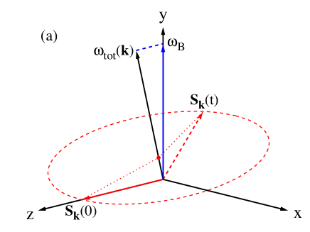
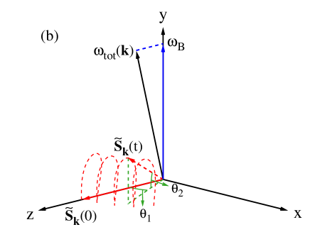
Figure 1: (Color online) The schematic illustration of the free spin precession in the case with the initial spin polarization along the $z$-axis in the Schrödinger (a) and interaction (b) pictures. The red dashed curves indicate the precession orbits. The red dotted lines in (a) connect the spin vectors ${\bf S}_{\bf k}(0)$ and ${\bf S}_{\bf k}(t)$ with the center of its precession orbit. Here we have exaggerated the angle between $\bm{\omega}_{\rm tot}({\bf k})$ and the $y$-axis in order to make the relevant precession angles more pronounced.

II Effective inhomogeneous broadening

To reveal the physics under the anomalous scaling of the DP SRT, we first discuss the effective inhomogeneous broadening by analysing the free spin precession between adjacent scattering events. Without scattering, the spin vector ${\bf S}_{\bf k}(t)$ just precesses around the total magnetic field $\bm{\omega}_{\rm tot}=\omega_{B}{\bf e}_{y}+\Omega_{z}({\bf k}){\bf e}_{z}$. Then one obtains

$${\bf S}_{\bf k}(t)=R_{\rm tot}(\omega_{\rm tot}({\bf k})t){\bf S}_{\bf k}(0),$$ (5)

in which $R_{i}(\phi)$ represents the rotation operator with angle $\phi$ around the direction ${\bf e}_{i}$. We take the case with the initial spin vector ${\bf S}_{\bf k}(0)$ along the $z$-axis as a typical example to schematically show the precession orbit in Fig. 1. It is seen that the main contribution of the precession angle is from the strong external magnetic field, which is momentum independent and hence does not contribute to the inhomogeneous broadening. To show the effective inhomogeneous broadening more clearly, we transform the spin vector into the interaction picture as $\tilde{\bf S}_{{\bf k}}(t)=R_{y}(-\omega_{B}t){\bf S}_{{\bf k}}(t)$, whose orbit is also plotted in Fig. 1. Then the spin evolution operator in the interaction picture $U_{\bf k}(t,0)$, defined as $\tilde{\bf S}_{{\bf k}}(t)=U_{\bf k}(t,0)\tilde{\bf S}_{{\bf k}}(0)$, can be obtained as

$$U_{\bf k}(t,0) = R_{y}(-\omega_{B}t)R_{\rm tot}(\omega_{\rm tot}({\bf k})t)$$ (6)

$$= R_{x^{\prime}(t)}(\beta_{\bf k})R_{y}(\omega_{\rm eff}({\bf k})t)R_{x}(-\beta_{\bf k}),$$

in which

$$\beta_{\bf k}\approx\tan\beta_{\bf k}=\Omega_{z}({\bf k})/\omega_{B},$$ (7)

$$\omega_{\rm eff}({\bf k})=\sqrt{\omega_{B}^{2}+\Omega_{z}^{2}({\bf k})}-\omega_{B}\approx\Omega_{z}^{2}({\bf k})/(2\omega_{B}),$$ (8)

$${\bf e}_{x^{\prime}(t)}=R_{y}(-\omega_{B}t){\bf e}_{x}=\cos(\omega_{B}t){\bf e}_{x}+\sin(\omega_{B}t){\bf e}_{z}.$$ (9)

In the above derivation, we have used the theorem $R_{j}(\theta_{j})R_{i}(\theta_{i})R_{j}(-\theta_{j})=R_{i^{\prime}}(\theta_{i})$ with ${\bf e}_{i^{\prime}}=R_{j}(\theta_{j}){\bf e}_{i}$ and the condition $\omega_{B}\gg\langle|\Omega_{z}({\bf k})|\rangle$. We further limit ourselves in the regime $\langle|\omega_{\rm eff}({\bf k})|\rangle t\sim\langle|\omega_{\rm eff}({\bf k})|\rangle\tau_{p}\ll 1$,valid thus all relevant rotation angles in Eq. (6) are very small and the corresponding rotation vectors satisfy the vector summation rule. Then one obtains the rotation vector $\bm{\theta}_{\bf k}(t,0)$, which corresponds to $U_{\bf k}(t,0)=\exp[-i{\bf J}\cdot\bm{\theta}_{\bf k}(t,0)]$ with ${\bf J}$ representing the angular momentum operator and

$$\bm{\theta}_{\bf k}(t,0) = \omega_{\rm eff}({\bf k})t\,{\bf e}_{y}+\beta_{\bf k}[\cos(\omega_{B}t)-1]{\bf e}_{x}$$ (10)

$${}+\beta_{\bf k}\sin(\omega_{B}t){\bf e}_{z}.$$

The above equation can also be understood with the help of Fig. 1. The first two terms in Eq. (10) just correspond to the angle between $\tilde{\bf S}_{{\bf k}}(0)$ [$\tilde{\bf S}_{{\bf k}}(0)={\bf S}_{{\bf k}}(0)$] and the projection of $\tilde{\bf S}_{{\bf k}}(t)$ in the $x$-$z$ plane ($\theta_{1}$) and the angle between $\tilde{\bf S}_{{\bf k}}(t)$ and the $x$-$z$ plane ($\theta_{2}$), respectively, illustrated in Fig. 1, while the third term is ineffective since $\tilde{\bf S}_{{\bf k}}(0)\parallel z$ in this case.

As mentioned above, all the relevant rotation angles are very small, thus the rotation vector between two adjacent scattering events occuring at $t$ and $t^{\prime}$ reads $\bm{\theta}_{\bf k}(t,t^{\prime})=\bm{\theta}_{\bf k}(t,0)-\bm{\theta}_{\bf k}(t^{\prime},0)$. Averaging over $\tau=t-t^{\prime}$ and $T=(t+t^{\prime})/2$, one obtains the mean square of the rotation angle between two adjacent scattering events in the case with the initial spin vector along ${\bf e}_{i}$,

$$\theta_{{\rm ave},i}^{2}({\bf k})=\int_{0}^{\tau_{p}}\frac{d\tau}{\tau_{p}}\int_{0}^{T_{B}}\frac{dT}{T_{B}}\Big{|}\overline{\bm{\theta}_{{\bf k}}(\tau,T)}-\overline{\bm{\theta}_{{\bf k}}(\tau,T)}\cdot{\bf e}_{i}{\bf e}_{i}\Big{|}^{2},$$ (11)

in which $T_{B}=2\pi/\omega_{B}$. Considering $T_{B}\ll\tau_{p}$, Eq. (11) reads

$$\theta_{{\rm ave},z}^{2}({\bf k}) = \frac{1}{\tau_{p}}\int_{0}^{\tau_{p}}d\tau\,\overline{\omega_{\rm eff}({\bf k})}^{2}\tau^{2}+\frac{4\beta_{\bf k}^{2}}{T_{B}^{2}}$$ (12)

$${}\times\int_{0}^{T_{B}}d\tau\int_{0}^{T_{B}}dT\;\sin^{2}(\omega_{B}\frac{\tau}{2})\sin^{2}(\omega_{B}T)$$

$$= \overline{\omega_{\rm eff}({\bf k})}^{2}\tau_{p}^{2}/3+\beta_{\bf k}^{2},$$

$$\theta_{{\rm ave},x}^{2}({\bf k}) = \overline{\omega_{\rm eff}({\bf k})}^{2}\tau_{p}^{2}/3+\beta_{\bf k}^{2},$$ (13)

$$\theta_{{\rm ave},y}^{2}({\bf k}) = 2\beta_{\bf k}^{2}.$$ (14)

Further exploiting the approximate formula of the DP SRT based on the random walk theory,opt-or

$$\tau_{s,i}^{-1}\sim\langle{\theta}_{{\rm ave},i}^{2}({\bf k})\rangle\tau_{p}^{-1},$$ (15)

one obtains the SRTs given by Eqs. (3) and (4). From the above discussions, one finds that the terms $\overline{\omega_{\rm eff}({\bf k})}^{2}\tau_{p}^{2}$ and $\beta_{\bf k}^{2}$ in Eqs. (12)-(14) describe two kinds of inhomogeneous broadening, which induce the DP-like ($\tau_{s}\propto\tau_{p}^{-1}$) and EY-like ($\tau_{s}\propto\tau_{p}$) behaviors, respectively. This is exactly the cause of the anomalous $\tau_{s}$-$\tau_{p}$ relations of the DP mechanism under a strong in-plane magnetic field.

III Investigations via KSBEs

In order to obtain the exact SRT, we turn to the fully microscopic KSBE approach.wu_review As mentioned in the introduction, we choose the investigated system to be the symmetric (110) QWs.Ohno_110 ; Wu_110 ; Dohrmann_04 ; spin_noise_110 ; Sherman_110 In fact, similar results can be obtained in (100) QWs with identical Dresselhaus and Rashba SOC strengthsAverkiev_identical ; Cheng and are not repeated here. The KSBEs can be written as

$$\partial_{t}{\rho}_{{\bf k}}=-i\left[\omega_{B}\frac{{\sigma}_{y}}{2}+\bm{\Omega}({\bf k})\cdot\frac{\bm{\sigma}}{2},\;\;{\rho}_{{\bf k}}\right]+\left.\partial_{t}{\rho}_{{\bf k}}\right|_{\rm scat},$$ (16)

in which $[\ ,\ ]$ denotes the commutator and ${\rho}_{\bf k}$ represents the density matrix of electron with momentum ${\bf k}$. The scattering term $\left.\partial_{t}{\rho}_{{\bf k}}\right|_{\rm scat}$ consists of the electron-impurity, electron–longitudinal-optical-phonon, electron–acoustic-phonon and electron-electron Coulomb scatterings with their expressions given in detail in Ref. Zhou_PRB_07, .

III.1 Analytic study

Before discussing the numerical results by solving the KSBEs, we first investigate the spin relaxation analytically in a simplified case, where only the linear-$k$ term in the Dresselhaus SOC and the elastic scattering (i.e., the electron-impurity scattering) are retained. Transforming the density matrix into the interaction picture as $\tilde{\rho}_{{\bf k}}=e^{iH_{B}t}\rho_{{\bf k}}e^{-iH_{B}t}$ and defining the spin vector

$$\tilde{\bf S}_{k,l}={\rm Tr}\big{[}\tilde{\rho}_{k,l}\bm{\sigma}\big{]},\qquad\tilde{\rho}_{k,l}=\frac{1}{2\pi}\int_{0}^{2\pi}d\phi_{\bf k}\tilde{\rho}_{\bf k}e^{il\phi_{\bf k}},$$ (17)

one obtains

$$\partial_{t}\tilde{\bf S}_{{\bf k},l}(t)=\tilde{U}_{\rm so}(t)\tilde{\bf S}_{{\bf k},l\pm 1}(t)-{\tilde{\bf S}_{{\bf k},l}(t)}/{\tau_{p,l}}.$$ (18)

Here

$$\tilde{U}_{\rm so}(t)=\Omega_{\rm so}\begin{pmatrix}0&-\cos\omega_{B}t&0\\ \cos\omega_{B}t&0&\sin\omega_{B}t\\ 0&-\sin\omega_{B}t&0\end{pmatrix}$$ (19)

in which $\Omega_{\rm so}=-{\gamma_{D}}\langle k_{z}^{2}\rangle_{0}k/4$ and

$${\tau_{p,l}^{-1}}=\frac{N_{i}}{2\pi}\int_{0}^{2\pi}d\phi_{\bf k}\;|W_{\rm ei}(k,\phi_{\bf k})|^{2}(1-\cos l\phi_{\bf k})$$ (20)

(note that $\tau_{p,1}=\tau_{p}$) with $W_{\rm ei}(k,\phi_{\bf k})$ standing for the matrix element of the electron-impurity scattering. Retaining terms with $|l|\leq 2$, Eq. (18) can be reduced into

$$\partial_{t}\tilde{\bf S}_{{\bf k},0}(t) =e^{-t/\tau_{p}}\tilde{U}_{so}(t)\int_{0}^{t}dt_{1}e^{t_{1}/\tau_{p}}\tilde{U}_{so}(t_{1})\Big{[}2\tilde{\bf S}_{{\bf k},0}(t_{1})$$

$${}+e^{-t_{1}/\tau_{p,2}}\int_{0}^{t_{1}}dt_{2}e^{t_{2}/\tau_{p,2}}\partial_{t_{2}}\tilde{\bf S}_{{\bf k},0}(t_{2})\Big{]}.$$ (21)

Next, we replace $\tilde{\bf S}_{{\bf k},0}(t_{1})$ by $\tilde{\bf S}_{{\bf k},0}(t)$ following the Markovian approximation and transform the above equation into the iterate form,

$$\partial_{t}\tilde{\bf S}_{{\bf k},0}(t)= \Big{\{}\Gamma_{1}(t)+{\cal F}[\Gamma_{1}(t)]+{\cal F}[{\cal F}[\Gamma_{1}(t)]]+...\Big{\}}\tilde{\bf S}_{{\bf k},0}(t),$$ (22)

$$\Gamma_{1}(t)= \;2e^{-t/\tau_{p}}\tilde{U}_{so}(t)\int_{0}^{t}dt_{1}e^{t_{1}/\tau_{p}}\tilde{U}_{so}(t_{1}),$$ (23)

$${\cal F}[g(t)]= \;e^{-t/\tau_{p}}\tilde{U}_{so}(t)\int_{0}^{t}dt_{1}e^{t_{1}/\tau_{p}}\tilde{U}_{so}(t_{1})$$

$$\times e^{-t_{1}/\tau_{p,2}}\int_{0}^{t_{1}}dt_{2}e^{t_{2}/\tau_{p,2}}g(t_{2}).$$ (24)

Further considering the magnitude of $\tilde{U}_{so}(t)$ is much smaller than its frequency $\omega_{B}$, we apply the rotating-wave approximation and only retain the terms with time-independent coefficients on the right side of Eq. (22). Then one obtains the SRTs, to the leading order,

$$\tau_{sz}^{-1}=\tau_{sx}^{-1}=\left\langle\frac{\overline{\Omega_{z}^{2}({\bf k})}^{2}\tau_{p,2}}{4\omega_{B}^{2}}+\frac{\overline{\Omega_{z}({\bf k})}^{2}\tau_{p}}{2(1+\omega_{B}^{2}\tau_{p}^{2})}\right\rangle,$$ (25)

$$\tau_{sy}^{-1}=\left\langle\frac{\overline{\Omega_{z}({\bf k})}^{2}\tau_{p}}{1+\omega_{B}^{2}\tau_{p}^{2}}\right\rangle.$$ (26)

Note that the factor $1/(1+\omega_{B}^{2}\tau_{p}^{2})$ also appears in the previous works on the spin relaxation under a magnetic field.Ivchenko_mag ; Margulis_mag ; Burkov_mag ; Glazov_mag In the strong-magnetic-field limit, $\omega_{B}\tau_{p}\gg 1$, one recovers Eqs. (3) and (4) from the above equations with $a=\tau_{p,2}/\tau_{p}$ and $b=b^{\prime}=1/2$. In addition, after considering the correction of the cubic Dresselhaus term, $\overline{\Omega_{z}({\bf k})}$ and $\overline{\Omega_{z}^{2}({\bf k})}$ in the above equations should be replaced by

$$\left.\Omega_{z}({\bf k})\right|_{l=1}=\frac{\gamma_{D}k}{8}\left({k^{2}}-4\langle k_{z}^{2}\rangle_{0}\right)\cos\phi_{\bf k}$$ (27)

and

$$\left.\Omega_{z}^{2}({\bf k})\right|_{l=2}=\frac{\gamma_{D}^{2}k^{2}}{128}\left({k^{2}}-4\langle k_{z}^{2}\rangle_{0}\right)\left(7{k^{2}}-4\langle k_{z}^{2}\rangle_{0}\right)\cos 2\phi_{\bf k},$$ (28)

respectively.

III.2 Numerical results

In this subsection, we investigate the exact SRT by numerically solving the KSBEs with all the scatterings explicitly included. We choose a symmetric (110) InAs QW due to its large Landé $g$ factor. For this material, $g=-14.3$Rocca_g_factor and $\gamma_{D}=-27.8$ eV Å³.Kotani_gamma_D The other material parameters can be found in Ref. para_semi, . We further set $B=2$ or $4$ T, both satisfying the condition $\omega_{B}\gg\langle|{\Omega_{z}({\bf k})}|\rangle$. The well width is chosen to be $a=5$ nm, which is smaller than the cyclotron radius of the lowest Landau level so that the orbital effect from the external magnetic field is irrelevant. It is noted that both the magnetic field and well width chosen here are within the experimental feasibility. In addition, the electron density is chosen to be $N_{e}=3\times 10^{11}$ cm^-2. The corresponding Fermi energy $E_{\rm F}\approx 30$ meV, which is much larger than the Zeeman splitting about $3$ meV for $B=4$ T. Therefore, the inclusion of the Zeeman splitting in the energy-conservation delta functions in the scattering terms of the KSBEs is unimportant to the relaxation of the out-of-equilibrium spin polarization we investigate.Cheng ; Grimaldi

We first compare the SRTs from the KSBEs with only the electron-impurity scattering with those from Eqs. (25) and (26) with the correction of the cubic Dresselhaus term. In Fig. 2, the results from these two approaches are plotted as the blue dashed and green chain curves for $B=4$ T in the case with the initial ensemble average spin polarization ${\bf P}=\sum\limits_{\bf k}{\bf S}_{\bf k}(0)/N_{e}$ along the $z$- and $y$-axes (recall ${\bf B}\parallel y$). The temperature and initial spin polarization are chosen to be $T=15$ K and $|{\bf P}|=0.1$ %. It is shown that the results from the numerical computations agree fairly well with the approximate formula in the impurity density regime satisfying $\tau_{p,2}^{-1}>\langle|\overline{\omega_{\rm eff}({\bf k})}|\rangle$ for the transverse SRT [${\bf P}\perp{\bf B}$, Fig. 2(a)], and in the whole impurity density regime for the longitudinal SRT [${\bf P}\parallel{\bf B}$, Fig. 2(b)]. This further justifies the validity of Eqs. (25) and (26) in these regimes, in consistence with the discussions presented above.tau_2

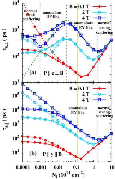
Figure 2: (Color online) Transverse (a) and longitudinal (b) SRTs from the calculations with all the relevant scatterings (solid curves) and only the electron-impurity scattering (dashed curves) against the impurity density under different magnetic fields. The green chain curves in (a) and (b) are the results from Eqs. (25) and (26), respectively. The vertical black dotted lines indicate the boundaries between different regimes under the strong magnetic field $B=4$ T. The vertical yellow lines indicate the boundary between the weak and strong scattering regimes in the weak field case.

From this figure, one also observes that the behaviors of the DP spin relaxation under a strong magnetic field (blue dashed curves) are very different from the conventional ones under a weak magnetic field (red solid curves). We first focus on the transverse SRT [Fig. 2(a)]. It is seen that the spin relaxation in this case can be divided into four regimes (separated by the vertical black dotted lines), in contrast to the two regimes in the weak field case, i.e., the weak and strong scattering regimes (separated by the vertical yellow solid line). The two regimes in the middle [$\tau_{p,2}\langle|\overline{\omega_{\rm eff}({\bf k})}|\rangle/\tau_{p}<\tau_{p}^{-1}<\omega_{B}$] are just the anomalous DP- and EY-like regimes discussed above, respectively. It is shown that, in the anomalous DP-like regime, which is in the original weak scattering limit, the DP SRT shows the strong scattering behavior ($\tau_{s}\propto\tau_{p}^{-1}$). Moreover, in the anomalous EY-like regime, most of which is in the original strong scattering limit, the DP SRT exhibits the EY-like behavior ($\tau_{s}\propto\tau_{p}$). All these anomalous behaviors come from the unique form of the inhomogeneous broadening given by Eq. (12), just as discussed above. A peak appears at the boundary between these two regimes, i.e., $\tau_{p}^{-1}=\sqrt{{\tau_{p,2}}\langle\overline{\Omega_{z}^{2}({\bf k})}^{2}\rangle/(2\tau_{p}\langle{\Omega_{z}^{2}({\bf k})}\rangle)}$, which is independent of the magnetic field. This effect comes from the competition of the two kinds of inhomogeneous broadening in Eq. (12). For lower (higher) impurity densities beyond the above regimes, the SRT exhibits the conventional DP behavior in the weak (strong) scattering limit. Thus we refer to these two regimes as the normal weak and strong scattering regimes, respectively. The behavior in the normal weak scattering regime can be understood by considering that the impurity scattering is too weak to suppress the inhomogeneous broadening from $\omega_{\rm eff}({\bf k})$ in Eq. (12), similar to the conventional weak scattering case. As for the normal strong scattering regime, the underlying physics is that when $\omega_{B}\tau_{p}\ll 1$, the inhomogeneous broadening returns to the conventional form, which can be demonstrated by exploiting Eq. (11) and considering $\sin(\omega\tau/2)\approx\omega\tau/2$ for $0<\tau<\tau_{p}$. We then turn to the longitudinal SRT [Fig. 2(b)]. There are only two regimes in this case. In the regime $\tau_{p}^{-1}<\omega_{B}$, the SRT decreases with increasing $N_{i}$, which comes from the inhomogeneous broadening given by Eq. (14), similar to the anomalous EY-like regime for the transverse SRT. In the regime $\tau_{p}^{-1}>\omega_{B}$, the SRT increases with $N_{i}$, because the inhomogeneous broadening returns to the conventional form, just as the normal strong scattering regime for the transverse SRT. Note that there is no normal weak scattering regime in this case. This is because when ${\bf P}\parallel y$, the term $R_{y}(\omega_{\rm eff}({\bf k})t)$ in the rotation matrix [Eq. (6)] does not contribute to the rotation anglerot_y and the corresponding rotation angles between adjacent scattering events become independent of $\tau_{p}$.

In Fig. 2, we also plot the SRT with only the impurity scattering for $B=2$ T as the azure dashed curve. It is shown that the SRT in this case is shorter than the corresponding one for $B=4$ T in the anomalous DP- and EY-like regimes but becomes very close to the latter one in the normal strong scattering regime, all of which are consistent with the form of the inhomogeneous broadening discussed above. It is also seen that in the case of ${\bf P}\perp{\bf B}$ [Fig. 2(a)], the areas of both the anomalous DP- and EY-like regimes for $B=2$ T are smaller than those for $B=4$ T, while the positions of the peak remain fixed. These behaviors are consistent with the above discussions on the boundaries between different regimes.

Then we discuss the SRTs with all the relevant scatterings. The results are plotted as the solid curves in Fig. 2. One observes that the behaviors in these cases are similar to the corresponding ones with only the electron-impurity scattering, especially all the anomalous behaviors in the anomalous DP- and EY-like regimes are retained with all scatterings included. This further justifies that these anomalous behaviors can be observed in experiments. It is also shown that the SRT with all scatterings is longer than that with only the impurity scattering in the anomalous DP-like regime for ${\bf P}\perp{\bf B}$, while shorter than the latter one in the anomalous EY-like regime for ${\bf P}\parallel{\bf B}$. All these behaviors are consistent with Eqs. (25) and (26). In addition, it is seen that the normal weak scattering regime, which previously appears at extremely low impurity for ${\bf P}\perp{\bf B}$, disappears in the impurity density dependence with all scatterings. This is because the condition $\tau_{p,2}^{-1}>\langle|\overline{\omega_{\rm eff}({\bf k})}|\rangle$ is always satisfied due to the inclusion of the other scatterings.

The anomalous scaling of the DP spin relaxation also significantly influences the temperature dependence of the SRT. The transverse and longitudinal SRTs are plotted as function of temperature for $N_{i}=0$ under different magnetic fields in Fig. 3. We first focus on the transverse SRT. The SRT under strong magnetic field first exhibits a valley and then a peak. The underlying physics is as follows. In the degenerate limit (i.e., $T\ll T_{\rm F}=E_{\rm F}/k_{\rm B}$ with $T_{\rm F}\approx 360$ K here), both the electron-electron and electron-phonon scatterings increase with increasing temperature, while the inhomogeneous broadening is insensitive to the temperature. Thus, the temperature dependence of the SRT is just determined by the momentum relaxation. As shown in Fig. 3, all the normal weak scattering, anomalous DP-like and EY-like regimes are in the degenerate limit. Therefore, the peak and valley appear around the boundaries between these three regimes, just similar to the impurity density dependence discussed above. However, it is also seen that no valley appears in the temperature dependence around the boundary between the anomalous EY-like and normal strong scattering regimes. This is because most of the normal strong scattering regime is in the nondegenerate limit ($T\gg T_{\rm F}$). In this limit, the scattering becomes insensitive to the temperature due to the competition of the decrease of the electron-electron scattering and the increase of the electron-phonon scattering, whereas the inhomogeneous broadening increases rapidly with the temperature. Thus, the SRT decreases with temperature in this regime. This leads to the absence of the valley. The SRT under weak magnetic field also shows first a valley and then a peak. But the positions of these valley and peak are quite different from the previous ones and the underlying physics is totally different. The valley can be understood by considering that the boundary between the weak and strong scattering regimes is in the degenerate limit. The peak is due to the crossover of the degenerate and nondegenerate limits in the strong scattering regime, which is well known in the literature.wu_review ; Zhou_PRB_07 Then we turn to the longitudinal SRT. It is seen that the behaviors under weak magnetic field are very similar to the corresponding transverse ones, but the behaviors under strong magnetic field become quite different: the SRT decreases monotonically with temperature. This is just because the system in this case belongs to the anomalous EY-like regime at low temperature.

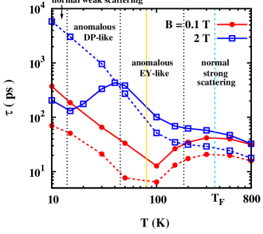
Figure 3: (Color online) Transverse (solid curves) and longitudinal (dashed curves) SRTs against the temperature for $N_{i}=0$ under different magnetic fields. The vertical azure dashed line indicates the temperature satisfying $T=T_{\rm F}$. The vertical black dotted lines separate the boundaries between different regimes for transverse SRT under the strong magnetic field $B=4$ T. The vertical yellow line illustrates the boundary between the weak and strong scattering regimes in the case of weak magnetic field.

IV Conclusion and Discussion

In conclusion, we have investigated the anomalous scaling of the DP SRT with the momentum relaxation time in semiconductor QWs under a strong magnetic field, whose direction is parallel to the QW plane and perpendicular to the spin-orbit field. We discover that, for the transverse SRT perpendicular to the magnetic field, the anomalous scaling occurs at two regimes, i.e., the anomalous DP- and EY-like regimes. In the anomalous DP-like regime, which is in the original weak scattering limit, the DP SRT is inversely proportional to the momentum relaxation time, i.e., the strong scattering behavior. On the other hands, in the anomalous EY-like regime, which is in the original weak scattering limit, the DP SRT is proportional to the momentum relaxation time, i.e, the EY-like behavior, both in the opposite trends against the conventional DP ones. As for the longitudinal SRT parallel to the magnetic field, the DP SRT is always proportional to the momentum relaxation time even in the original strong scattering limit, similar to the anomalous EY-like regime for the transverse SRT. We further demonstrate that all these anomalous scaling relations come from the unique form of the effective inhomogeneous broadening.

Finally, we address the choice of the material. In the above calculations, we choose InAs (110) QWs. In fact, similar behaviors also appear in (110) QWs made of the other materials with large Landé $g$ factor, e.g., InSbpara_semi , and (100) QWs with identical Dresselhaus and Rashba strengths made of InAs and InSb. However, the situation becomes very different for QWs made of materials with small $g$ factor, e.g., GaAs, since the conditions $\omega_{B}\gg\langle|{\Omega_{z}({\bf k})}|\rangle$ and the well width is smaller than the cyclotron radius of the lowest Landau level cannot be satisfied simultaneously.

- (1) F. Meier and B. P. Zakharchenya, Optical Orientation (North-Holland, Amsterdam, 1984).
- (2) Semiconductor Spintronics and Quantum Computation, edited by D. D. Awschalom, D. Loss, and N. Samarth (Springer-Verlag, Berlin, 2002); I. Žutić, J. Fabian, and S. Das Sarma, Rev. Mod. Phys. 76, 323 (2004); J. Fabian, A. Matos-Abiague, C. Ertler, P. Stano, and I. Žutić, Acta Phys. Slov. 57, 565 (2007); Spin Physics in Semiconductors, edited by M. I. D’yakonov (Springer, Berlin, 2008); Handbook of Spin Transport and Magnetism, edited by E. Y. Tsymbal and I. Žutić (Chapman & Hall/CRC, Boca Raton, 2011).
- (3) M. W. Wu, J. H. Jiang, and M. Q. Weng, Phys. Rep. 493, 61 (2010).
- (4) Y. Yafet, Phys. Rev. 85, 478 (1952); R. J. Elliott, ibid. 96, 266 (1954).
- (5) M. I. D’yakonov and V. I. Perel’, Zh. Eksp. Teor. Fiz. 60, 1954 (1971) [Sov. Phys. JETP 33, 1053 (1971)]; Fiz. Tverd. Tela (Leningrad) 13, 3581 (1971) [Sov. Phys. Solid State 13, 3023 (1972)].
- (6) M. W. Wu and C. Z. Ning, Eur. Phys. J. B 18, 373 (2000); M. W. Wu, J. Phys. Soc. Jpn. 70, 2195 (2001).
- (7) G. Dresselhaus, Phys. Rev. 100, 580 (1955).
- (8) Y. A. Bychkov and E. I. Rashba, J. Phys. C 17, 6039 (1984); JETP Lett. 39, 78 (1984).
- (9) N. Tombros, S. Tanabe, A. Veligura, C. Józsa, M. Popinciuc, H. T. Jonkman, and B. J. van Wees, Phys. Rev. Lett. 101, 046601 (2008); M. Popinciuc, C. Józsa, P. J. Zomer, N. Tombros, A. Veligura, H. T. Jonkman, and B. J. van Wees, Phys. Rev. B 80, 214427 (2009); C. Józsa, T. Maassen, M. Popinciuc, P. J. Zomer, A. Veligura, H. T. Jonkman, and B. J. van Wees, ibid. 80, 241403(R) (2009).
- (10) K. Pi, W. Han, K. M. McCreary, A. G. Swartz, Y. Li, and R. K. Kawakami, Phys. Rev. Lett. 104, 187201 (2010); W. Han and R. K. Kawakami, ibid 107, 047207 (2011).
- (11) A. Avsar, T. Y. Yang, S. Bae, J. Balakrishnan, F. Volmer, M. Jaiswal, Z. Yi, S. R. Ali, G. Giintherodt, B. H. Hong, B. Beschoten, and B. Özyilmaz, Nano Lett. 11, 2363 (2011).
- (12) S. Jo, D. K. Ki, D. Jeong, H. J. Lee, and S. Kettemann, Phys. Rev. B 84, 075453 (2011).
- (13) P. Zhang and M. W. Wu, New J. Phys. 14, 033015 (2012).
- (14) Y. Ohno, R. Terauchi, T. Adachi, F. Matsukura, and H. Ohno, Phys. Rev. Lett. 83, 4196 (1999); Physica E 6, 817 (2000); T. Adachi, Y. Ohno, F. Matsukura, and H. Ohno, Physica E 10, 36 (2001).
- (15) M. W. Wu and M. Kuwata-Gonokami, Solid State Commun. 121, 509 (2002).
- (16) S. Döhrmann, D. Hägele, J. Rudolph, M. Bichler, D. Schuh, and M. Oestreich, Phys. Rev. Lett. 93, 147405 (2004).
- (17) G. M. Müller, M. Römer, D. Schuh, W. Wegscheider, J. Hübner, and M. Oestreich, Phys. Rev. Lett. 101, 206601 (2008).
- (18) I. V. Tokatly and E. Y. Sherman, Phys. Rev. B 82, 161305(R) (2010).
- (19) In fact, the contribution from the homogeneous part of in the rotation matrix given by Eq. (6) can be removed through the transformation . Thus, the valid condition of Eq. (3) is , as presented at the beginning of this investigation.
- (20) N. S. Averkiev and L. E. Golub, Phys. Rev. B 60, 15582 (1999).
- (21) J. L. Cheng and M. W. Wu, J. Appl. Phys. 99, 083704 (2006).
- (22) J. Zhou, J. L. Cheng, and M. W. Wu, Phys. Rev. B 75, 045305 (2007); see also page 136 in Ref. wu_review, .
- (23) E. L. Ivchenko, Fiz. Tverd. Tela (Leningrad) 15, 1566 (1973) [Sov. Phys. Solid State 15, 1048 (1973)].
- (24) A. D. Margulis and V. A. Margulis, Fiz. Tverd. Tela (Leningrad) 25, 1590 (1983) [Sov. Phys. Solid State 25, 918 (1983)].
- (25) A. A. Burkov and L. Balents, Phys. Rev. B 69, 245312 (2004).
- (26) M. M. Glazov, Phys. Rev. B 70, 195314 (2004).
- (27) J.-M. Jancu, R. Scholz, E. A. de Andrada e Silva, and G. C. La Rocca, Phys. Rev. B 72, 193201 (2005).
- (28) A. N. Chantis, M. van Schilfgaarde, and T. Kotani, Phys. Rev. Lett. 96, 086405 (2006).
- (29) Semiconductors, edited by O. Madelung (Springer-Verlag, Berlin, 1987), Vol. 17a.
- (30) C. Grimaldi, Phys. Rev. B 72, 075307 (2005).
- (31) It is reasonable to replace in the original validity condition of Eq. (3) by , as is exactly the momentum relaxation time related to the inhomogeneous broadening from , shown in the angular expansion of the KSBEs.
- (32) This fact can be seen by transforming Eq. (6) into the form with .