Magnetic field-induced giant enhancement of electron-phonon energy transfer in strongly disordered conductors.

Abstract

Relaxation of soft modes (e.g. charge density in gated semiconductor heterostructures, spin density in the presence of magnetic field) slowed down by disorder may lead to giant enhancement of energy transfer (cooling power) between overheated electrons and phonons at low bath temperature. We show that in strongly disordered systems with time-reversal symmetry broken by external or intrinsic exchange magnetic field the cooling power can be greatly enhanced. The enhancement factor as large as $10^{2}$ at magnetic field $B\sim 10$ Tesla in 2D InSb films is predicted. A similar enhancement is found for the ultrasound attenuation.

Introduction– A number of recent experiments show that energy transfer (the cooling power) $\mathcal{J}(T_{e},T_{ph})=J(T_{el})-J(T_{ph})$ between overheated electrons with temperature $T_{el}>T_{ph}$ and phonons at low bath temperature $T_{ph}$ may vary by several orders of magnitude when measured per one electron per volume. The out-flux $J(T)=W\,T^{p}$ may have different power-law temperature dependence with the exponent $p$ both smaller and larger than the classical result $p=5$ valid for pure metals. In disordered metals with complete screening of Coulomb interaction and impurities that are fully involved in the lattice motion one expects  schmid ; reyzer ; kravtsov_yudson a power law with $p=6$ which corresponds to weaker energy transfer compared to the clean case. This is related with the ”Pippard ineffectiveness condition”  (denoted as PIC below) pippard ; akhiezer formulated for the rate of inelastic electron-phonon scattering. A very accurate experiments in metal films of Hf and Ti Gersh2001 confirmed this theoretical expectation, including the value of the pre-factor $W$ in front of $T^{6}$. At the same time, experiments on heavily doped SiPekola2004 which also demonstrated the $T^{6}$ behavior, gave at low temperatures the value $W/n_{e}$ ($n_{e}$ is the carrier density) larger by a factor of $10^{3}$ than the theoretical prediction in Ref.schmid ; reyzer ; kravtsov_yudson . Surprisingly, the $T^{6}$ behavior of the cooling rate with approximately the same values of $W/n_{e}$ as in Ref.Pekola2004 were extracted from the recent experiments Sacepe2009 on amorphous InO films showing weakly insulating behavior in magnetic field of 11T. In this case $W/n_{e}$ was larger by a factor of $5\times 10^{4}$ than the theoretical prediction for a dirty metal approaching the Anderson transition. Clearly, neither of the above cases with anomalously large cooling rate correspond to the piezoelectric type of electron-phonon coupling where the PIC does not hold and the theory predicts $T^{4}$ temperature behavior of cooling rate piezo ; Gersh2000 . It is also dubious that the model of impurities which are only partially involved in the lattice motion reyzer that also leads to enhanced cooling rate with $T^{4}$ temperature behavior, is realistic for the cases in question. Thus there was a quest from experiment for a different and more general mechanism of enhancement of cooling rate in strongly disordered conductors.

In the present Letter we demonstrate existence of a general mechanism which is capable of enhancing by a factor $10^{2}-10^{3}$ of both the cooling power $J(T)$ and ultrasound attenuation $\tau^{-1}_{ph}$ (for longitudinal phonons) at low temperatures. This mechanism is effective if lattice motion is able to induce significant oscillations of local densities of certain globally conserved physical quantities. The deviations of these local densities from their equilibrium values are enhanced by slow diffusive character of electron motion (characterized by both small frequency and small momentum) aimed to restore equilibrium. This leads to a significant retardation in the response and thus to the entropy production and dissipation. The proposed mechanism is reminiscent of the Mandelstam-Leontovich (ML) mechanism of phonon attenuation in liquids MLref . In contrast to PIC which suppresses the relaxation rate $\tau_{ph}^{-1}$ at strong disorder and small carrier concentration, the ML mechanism is efficient at these conditions. The particular realizations of such a mechanism were studied previously in the literature. Specifically, relatively weak Coulomb interaction between electrons in semiconductors, when the local electroneutrality condition is not strictly obeyed and the density fluctuations are not completely suppressed, was a cause of enhancement of cooling rate discussed in Ref.Reizer_screening . The asymmetric inter-valley modes were shown Prunnila to lead to a significant enhancement of cooling rate in multiple-valley semiconductors such as ${\rm Si}$. Below we reproduce some of these results from our general approach.

However, a really new effect we are predicting is the giant enhancement of the cooling rate and ultra-sound attenuation in the presence of external magnetic field or in ferromagnetic materials where the role of external magnetic field is played by the intrinsic exchange field. In this case it is the spin-density mode which can be excited by absorption of a phonon or terminated by creation of a phonon, that is responsible for the enhanced ultrasound attenuation or the enhanced cooling rate.

Cooling power and ultrasonic attenuation– The starting point of our consideration is the quantum kinetic equation SerMit ; apps for the phonon distribution function $B_{ph}(\omega,T)$. for the case of partial equilibrium in the electronic (with the temperature $T_{el}$) and phonon (with the temperature $T_{ph}$) systems at the lack of the total equilibrium ($T_{el}>T_{ph})$:

$$\partial_{t}B_{ph}(\omega,T_{ph})=\left[B_{ph}(\omega,T_{el})-B_{ph}(\omega,T_{ph})\right]\cdot\tau^{-1}_{ph}\left(\omega,T_{el}\right).$$ (1)

If the electron-phonon energy relaxation is much slower than the electron-electron one and the phonon system is well coupled to the thermostat (fridge), a quasi-equilibrium situation with two temperatures is realized. In this approximation $B_{ph}(\omega,T)\equiv B_{ph}(\omega/T)=\frac{1}{2}(\coth(\omega/2T)-1)$ is the equilibrium phonon distribution function. The phonon decay rate $\tau^{-1}_{ph}$ is then given by the imaginary part of the phonon self-energy $\Sigma^{R}(\omega,q,T)$:

$$\tau^{-1}_{ph}(\omega,T_{el})=\frac{1}{\rho_{m}\,\omega}\,{\rm Im}\Sigma^{R}(\omega,q,T_{el})|_{\omega=v_{s}q}.$$ (2)

The phonon decay rate depends only on the electron temperature, since the (weak) electron-phonon interaction is considered in the leading approximation, and thus the phonon self energy (which is second order in the e-ph coupling) is expressed in terms of electronic variables only. If in addition, the effect of electron-electron interaction is reduced to charge screening considered in the RPA approximation, the phonon relaxation rate $\tau^{-1}_{ph}(\omega,T_{el})\equiv\tau^{-1}_{ph}(\omega)$ does not depend explicitly on the electron temperature.

Now the energy flow $\mathcal{J}=\frac{dE_{ph}}{dt}$ from hot electrons to cool phonons can be written as follows $\mathcal{J}=J(T_{el})-J(T_{ph})$, where:

$$J(T)=\int\limits_{0}^{\infty}d\omega\,\omega\,\nu_{ph}(\omega)\,\frac{B_{ph}(\omega/T)}{\tau_{ph}(\omega)}$$ (3)

and $\nu_{ph}(\omega)=\omega^{2}/(2\pi^{2}v_{s}^{3})$ is the phonon density of states for 3D phonons with the sound velocity $v_{s}$. Eqs.(2),(3) establish a relationship between the cooling rate $J(T)$ and the attenuation time $\tau_{ph}(\omega)$ of ultrasound with the frequency $\omega$. In particular, it follows from Eq.(3) that for the power-law dependence $\tau^{-1}_{ph}(\omega)\propto\omega^{\beta}$, the cooling rate due to 3D phonons is proportional to $J(T)\propto T^{4+\beta}$.

Local and diffusion contribution to cooling rate– In impure conductors there are two distinctly different contributions to the phonon relaxation time. One is local and determined by the small distances $|{\bf r}-{\bf r^{\prime}}|\sim l$ between the points ${\bf r}$ and ${\bf r^{\prime}}$ of phonon absorption and re-emission. The other one allows many scattering events of electrons off impurities between the points ${\bf r}$ and ${\bf r^{\prime}}$. This is the diffusive contribution. With increasing disorder and decreasing the mean free path $l$ the local contribution diminishes. This leads to the so called Pippard inefficiency condition (PIC) when the relaxation rate $\tau^{-1}_{ph}(\omega)$ of phonons with momentum $q$ is proportional to $lq^{2}\ll q$ instead of $\tau_{ph}^{-1}\propto q$ for longitudinal phonons in the clean case pippard ; akhiezer :

$$\frac{1}{\tau^{(PIC)}_{ph}(\omega)}=c_{\alpha}\frac{2\nu p_{F}^{2}}{\rho_{m}}Dq^{2}\sim\frac{m\,n_{e}}{\rho_{m}}\,Dq^{2},$$ (4)

where $\nu$ is an electron density of states per spinnu , $p_{F}=mv_{F}$ is Fermi momentum, $n_{e}$ and $\rho_{m}$ are the density of electrons and the mass density of material, $D=v_{F}l/d_{e}$ is the diffusion coefficient, $q=\omega/v_{s}\ll 1/l$ is the phonon momentum, $d_{e}$ is the dimensionality of electron motion. The subscript $\alpha$ corresponds to the choice of either transverse (tr) or longitudinal (l) phonons; correspondingly, numerical coefficients $c_{\alpha}$ are defined as $c_{tr}=1/(2+d_{e})$ and $c_{l}=2(1-d_{e}^{-1})/(2+d_{e})$.

The diffusion contribution has an opposite trend and increases with increasing disorder. The goal of our paper is to analyze this very contribution in different physical situations.

We will use the co-moving frame of reference (CFR) bound to the lattice and impurities rigidly imbedded in it and moving in the laboratory frame of reference (LFR). Then for a single branch of electrons, one finds blount ; schmid for electron-phonon interaction in the CFR:

$$H_{e-ph}=-\sum_{{\bf p},{\bf q}}p_{\alpha}(v_{\beta}\nabla_{\beta}u_{\alpha})_{q}\cdot\bar{\psi}_{p}\psi_{p+q}$$ (5)

where ${\bf p}$ and ${\bf v}$ denote electron momentum and velocity, respectively and ${\bf u}$ is the lattice displacement. Note that this term appears due to the inhomogeneous Galilean shift ${\bf p}\,d{\bf u}({\bf r}(t),t)/dt$ of the energy of a quasi-particle at a point ${\bf r}={\bf r}(t)$, while the usual deformation potential in LFR is canceled by the modification of ${\rm e-e}$ interaction due to inhomogeneous coordinate transformation tsuneto $\widehat{H}\rightarrow\widehat{U}^{-1}\widehat{H}\widehat{U}$ with $\widehat{U}=1+\frac{1}{2}\{{\bf u},\boldsymbol{\nabla}\}$. The tensor structure of Eq.(5) is crucial for local processes only, while for diffusion processes, it is sufficient to average the e-ph vertex over the Fermi surface. For a metal with isotropic electron dispersion one finds $\Gamma=\overline{p_{\alpha}(v_{\beta}\nabla_{\beta}u_{\alpha})_{q}}=pv/d_{e}\,{\rm div}{\bf u}$. In general $\Gamma$ may contain other contributions. In particular, for semiconductors $\Gamma$ is known dp_semiconductors to be much larger than $E_{F}$ due to contribution $\Gamma_{bs}$ originating from the shift of conduction band-edge $E_{b}$.

Under the condition of strict electroneutrality, the scalar vertex $\Gamma$ is screened out completely and the classical result Eq.(4) is valid. This is not the case, however, when $N$ different types of quasiparticles are present Prunnila . Then the interaction can be written as

$$H_{e-ph}=\sum_{j=1}^{N}\Gamma^{(j)}\,{\rm div}{\bf u}\;(\bar{\psi}\psi)_{j},$$ (6)

where ($\nu_{j}$ is the partial DoS at the Fermi level):

$$\Gamma^{(j)}=-p^{(j)}v^{(j)}/d_{e}+\Gamma_{bs}.$$ (7)

Note that Eq.(6) is principally different from the ${\rm e-ph}$ interaction in the LFR, even when $\Gamma_{bs}=0$. The latter contains the deformation potential $\Gamma_{def}=\sum_{j}\nu_{j}\,(p_{F}^{(j)}v_{F}^{(j)}/d_{e})/\sum_{j}\nu_{j}$ which is symmetric in the electron branch indices $j$, as well as the moving-impurity part schmid ; reyzer ; kravtsov_yudson . The latter part leads to the mode-asymmetry of ${\rm e-ph}$ interaction in LFR which in CFR is provided by the Galilean shift term.

The Coulomb interaction is able to screen out only the single mode corresponding to the total density $n=\sum_{j}(\bar{\psi}\psi)_{j}$, whereas $N-1$ asymmetric modes survive screening Prunnila ; blount . Their slow, diffusive character in strongly disordered conductors may lead to a considerable enhancement of the cooling rate and ultrasound attenuation. The particular case of the effect of such unscreened diffusion modes was studied in Ref.Prunnila for the case of $N$ species of electrons corresponding to N inequivalent valleys in semiconductors.

Below we present a simple derivation of the diffusion-enhanced contribution to the phonon relaxation rate $\tau^{-1}_{ph}$ in terms of macroscopic equations for the current and density of electrons; alternative diagrammatic derivation is presented in supplementary , Sec. III. In the CFR the continuity and diffusion equations for each i-th species of quasiparticles read:

$$\left\{\begin{aligned} &\partial_{t}n^{(i)}+\mathrm{div}{\bf j}^{(i)}=0,\\ &{\bf j}^{(i)}=-D{\bf\nabla}n^{(i)}-\kappa_{i}{\bf F}^{(i)}\end{aligned}\right.$$ (8)

where $(i)$ stands for the quasiparticle branch number, $n^{(i)}$ is the electron density, ${\bf j}^{(i)}$ is the particle number current, $\kappa_{i}=\nu_{i}D_{i}$ is the mobility, $D_{i}$ is the diffusion coefficient for the $i$-th branch, ${\bf F}^{(i)}=-\nabla U^{(i)}$ and $U^{(i)}$ is the potential energy. In the simplest derivation we assume no inter-branch mixing and thus the continuity equations in Eq.(8) imply that each of the partial electron densities $n^{(i)}$ are conserved separately. Generalization to the case where there is mixing between the branches will be done at the end of the paper. The potential energy $U^{(i)}=U_{C}+\Phi^{(i)}$ in Eq.(8) consists of the Coulomb part $U_{C}$ and the phonon part $\Phi^{(i)}=\Gamma^{(i)}\,{\rm{div}\bf{u}}$:

$$U^{(i)}=\int{\cal V}_{0}({\bf r}-{\bf r}^{\prime})\sum\limits_{j}\delta n^{(j)}({\bf r}^{\prime})+\Gamma^{(i)}\,{\rm{div}\bf{u}}$$ (9)

where ${\cal V}_{0}({\bf r})$ is the bare Coulomb potential acting between conduction electrons; below we use its Fourier-transform $V_{0}(q)$. Note that $V_{0}(q)$ does not include screening by conduction electrons in the sample.

Eqs.(8),(9) is a full set of equations describing the diffusion and screening of partial densities $n_{i}$. Let us first study their solution in the case of perfect screening and multiple electron branches ($N>1$). It formally corresponds to $\Pi(\omega,q)\,V_{0}(q)\gg 1$, where $\Pi(\omega,q)$ is the total polarization function. For the density modulation $n^{(i)}(\omega,q)$ induced by the phonon with frequency $\omega$ and momentum $q$ one finds from Eqs.(8,9):

$$n^{(i)}(\omega,q)=\Pi_{i}(\omega,q)\left(\Phi_{i}(\omega,q)-\Phi_{C}(\omega,q)\right)$$ (10)

where $\Phi_{i}(\omega,q)=\Gamma^{(i)}\,{\rm{div}\bf{u}}$ , $\Phi_{C}={\sum_{j}\Phi_{j}\Pi_{j}}/\sum_{j}\Pi_{j}$ represents dynamical screening of Coulomb interaction and $\Pi_{i}=\nu_{i}D_{i}q^{2}/(-i\omega+D_{i}q^{2})$ is the partial polarization function. The solution Eq.(10) obeys charge-neutrality: $n_{tot}=\sum n^{(i)}=0$.

The diffusion contribution to the phonon decay rate may be expressed as $\tau_{ph,ML}^{-1}=\frac{|Q_{t}|}{E_{w}}$, where $Q_{t}$ and $E_{w}$ are the dissipation power and the acoustic wave energy in a unit volume, respectively:

$$Q_{t}=\frac{1}{2}{\rm\,Re\,}\left({\bf j}^{*}\cdot{\bf F}\right)\,,\qquad E_{w}=\frac{\rho_{m}}{2}\omega^{2}u_{m}^{2}.$$ (11)

Here $u_{m}$ is an amplitude of ionic displacement and ${\bf u}=({\bf q}/q)u_{m}\exp[-i\omega t+i{\bf q}\cdot{\bf r}]$. Below we apply Eq.(11) to compute $\tau_{ph}^{-1}(\omega)$.

Giant enhancement by magnetic field– The case of $N=2$ quasiparticle branches has a very important application. It corresponds to the two spin projections. However, they should be inequivalent with respect to the coupling to phonons. This is a consequence of the general statement that the spin density can be excited by phonons only if time-reversal invariance (TRI) is broken. First, we discuss the case when TRI is broken by external magnetic field.

For $N=2$ a simple calculation based on Eqs. (10),(11) leads to the following expression for the diffusion contribution to the decay rate of acoustic phonon:

$$\tau_{ph}^{-1}(q)=\frac{\left(\Gamma_{1}-\Gamma_{2}\right)^{2}}{\rho_{m}}\frac{\nu_{*}D_{*}q^{2}}{v_{s}^{2}+D_{*}^{2}q^{2}}$$ (12)

where $v_{s}=\omega/q$ is the sound velocity, while $\nu_{*}=(\nu_{1}^{-1}+\nu_{2}^{-1})^{-1}$ and $D_{*}=\nu_{*}^{-1}((\nu_{1}D_{1})^{-1}+(\nu_{2}D_{2})^{-1})^{-1}$ are the effective density of states and diffusion coefficient, respectively.

When a parallel magnetic field $H$ is applied to a two-dimensional electron gas the bottom of the spin-down and spin-up conduction bands get shifted by $\pm(1/2)\mu H$ with respect to their position at $H=0$. This leads to a change of $\delta(p_{F}v_{F})=\pm\mu H$, where $(1/2)\mu=(g/2)\mu_{B}$ is the electron magnetic moment. Thus from Eq.(7) we conclude that an asymmetry $\Gamma_{\uparrow}-\Gamma_{\downarrow}=(2/d_{e})\,\mu H$, arises due to the Galilean shift of the quasi-particle energy. Then, according to Eq.(12), the phonon relaxation rate acquires an $H$-dependent contribution that may become dominant at sufficiently strong field and low phonon frequencies. Adding the local contribution (4) and the magnetic-field-controlled diffusion contribution, Eq.(12), one finds for the full phonon decay rate $\tau_{ph}^{-1}=[\tau^{(PIC)}_{ph}]^{-1}\cdot\mathcal{F}_{H}(q,h)$, where for ${\bf q}$ parallel to 2D gas:

$$\mathcal{F}_{H}(q,h)=1+\frac{v_{F}^{2}h^{2}}{v_{s}^{2}+(Dq)^{2}}.$$ (13)

Here $\tau^{(PIC)}_{ph}$ is given by Eq.(4) for longitudinal phonons and $h=(|\mu|H/2\varepsilon_{F})$   (we assume here $h\ll 1$). The enhancement factor $\mathcal{F}_{H}$ can become very large for strong spin polarization, $h\sim 1$. In particular, for low phonon momentum, $ql\leq v_{s}/v_{F}$, the factor $\mathcal{F}_{H}$ is of the order of inverse adiabatic parameter $(v_{F}/v_{s})^{2}\sim 10^{5}$. The strong spin-orbit interaction which leads to mixing of spin-up and spin-down branches sets limitation on the enhancement factor. Its maximum value becomes ${\cal F}_{max}\sim\tau_{SO}/\tau$ ($\tau_{SO}$ is the spin relaxation time and $\tau\ll\tau_{SO}$ is the momentum relaxation time) instead of ${\cal F}_{m}\sim(v_{F}/v_{s})^{2}$. This makes the optimization of parameters to maximize the enhancement factor a hard problem, since materials with large $g$-factor (to maximize $\mu H$) usually have large spin-orbit coupling. Nevertheless the example of ${\rm InSb}$ films shows that ${\cal F}\sim 10^{2}$ is experimentally achievable (see Fig.1).

Enhancement of cooling rate in ferromagnetic metals– Another relevant example is provided by ferromagnetic metals with strong intrinsic band-splitting due to the exchange field. In the case of $\mathrm{Fe}$: $\mu H^{*}\approx 1.8\,\mathrm{eV},\,\varepsilon_{F}=11.1\,\mathrm{eV},\,v_{F}=1.98\times 10^{8}\mathrm{cm/s},\,v_{s}\approx 6\times 10^{5}\mathrm{cm/s}$. The spin relaxation rate may be estimated as $\tau/\tau_{SO}\sim(\alpha Z)^{4}\sim 10^{-3}$, $\alpha=1/137$ and $Z=26$ being the fine structure constant and the atomic number respectively, resulting in the maximum enhancement of the phonon relaxation time as large as $\mathcal{F}_{H}\sim(\mu H^{*}/\varepsilon_{F})^{2}\,(\tau_{SO}/\tau)\sim 10$.

Enhancement by incomplete screening. In the case of a single quasipaticle branch, the general approach Eqs.(8),(9),(11) describes the diffusion-enhanced dissipation due to violation of the charge neutrality condition at a large screening length. In this case we obtain $n=2\nu Dq^{2}\left[-i\omega+Dq^{2}+2\kappa\,q^{2}\,V_{0}(q)\right]^{-1}\,\Phi(\omega,q)$ and the enhancement factor:

$$\mathcal{F}_{C}=1+\frac{c_{l}^{-1}(\Gamma/p_{F}v_{F})^{2}}{(v_{s}/v_{F})^{2}+d_{e}^{-2}(q^{2}l^{2})(1+2\nu V_{0}(q))^{2}}$$ (14)

For the 2D gas with Coulomb interaction and the constant dielectric permittivity $\varepsilon$ of surrounding media we have $V_{0}(q)=V_{2D}(q)=2\pi e^{2}/\varepsilon q$. In the relevant range of ${\bf q}$ parallel to the 2D gas the $\mathcal{F}_{C}(q)$ factor reduces to a constant. This corresponds to the cooling rate $J(T)\propto T^{6}$ Reizer_screening but with the enhanced pre-factor proportional to $\varepsilon^{2}/g_{\Box}^{2}$ (where $g_{\Box}$ is dimensionless conductance per square in $e^{2}/h$ units) at strong disorder and large dielectric constant $\varepsilon$. In 3D conductors, when $V_{0}(q)\propto q^{-2}$ Eq.(14) has a regime were ${\cal F}_{C}\propto q^{2}$. Correspondingly, the cooling rate appears to be $J(T)\propto T^{8}$ Reizer_screening .

An interesting situation arises in 2D electron gas in the presence of a gate that additionally screens Coulomb interaction and allows the density to fluctuate stronger. For this geometry and ${\bf q}$ parallel to 2D gas $V_{0}(q)\rightarrow V_{g}(q)=V_{2D}(q)\,(1-e^{-2qb})$, $b$ being the distance between the 2d electron gas and the gate. For phonons with the wavelengths $1/q\geq b$, the effective potential $V_{g}(q)\approx V(q)\cdot 2qb\approx const$ and the presence of adiabatic parameter in the denominator of (14) does become important at low enough temperatures:

$$\mathcal{F}_{C_{gate}}=1+\frac{4(\Gamma/p_{F}v_{F})^{2}}{(v_{s}/v_{F})^{2}+(q^{2}l^{2})(4\pi\nu e^{2}b/\varepsilon)^{2}},$$ (15)

where Coulomb interaction is still assumed to be relatively strong: $2\pi\nu e^{2}b/\varepsilon\gg 1$. In this case there is a regime where the enhancement factor is proportional to $q^{-2}$, and the cooling rate $J(T)\propto T^{4}$.

Modes mixing and realistic example– Finally, we collect results of both the ML enhancement due to the charge density and the spin density fluctuations, taking also into account mixing of spin projections by the spin-orbit interaction characterized by the parameter $\tau_{so}^{-1}$. We also consider the dependence of relaxation rate on the direction of phonon propagation relative to 2D gassupplementary . Both effects lead to the replacement $Dq^{2}/(-i\omega+Dq^{2})\Rightarrow D{\bf q}_{\parallel}^{2}/(-i\omega+D{\bf q}_{\parallel}^{2}+1/2\tau_{so})$. It results in the total enhancement factor of the form:

$${\cal F}={\cal F}_{C_{2D}}+\frac{{\bf q}^{2}_{\parallel}v_{F}^{2}h^{2}}{(qv_{s})^{2}+(D{\bf q}_{\parallel}^{2}+1/2\tau_{so})^{2}}$$ (16)

For 2D electrons and 3D phonons $|{\bf q}_{\parallel}|=q\,\sin\theta$ is the phonon momentum component parallel to the 2D system which appears in all the terms originating from electron diffusion. In this case ${\cal F}_{C_{2D}}$ is independent of $q$, and ${\cal F}$ has a maximum as a function of $\omega$. The spin fluctuation effect given by the second term vanishes at small $\omega$ because of the mixing of branches caused by spin-orbit interaction. It also decreases at large $\omega$ because the dissipation power increases slower with $\omega$ than does the acoustic wave energy. At large enough Zeeman splitting $h$ when the effect of spin fluctuations in its maximum is large, there is a wide frequency region (the falling part of the curve ${\cal F}\propto\omega^{-2}$ in Fig.1) where $\tau_{ph}^{-1}$ is almost frequency independent. In this region the cooling/heating rate $J(T)\propto T^{4}\,\ln T$ for the quasi-2D case. This temperature dependence is almost the same as in the case of impurities which are not fully involved in the lattice motion static_disorder . The extra logarithmic factor arises because of the angular averaging of $1/\tau_{ph}(\theta)$ dominated by the small values of $\theta$. To illustrate this behavior we consider a thin film of semiconductor $\mathrm{InSb}$ (g-factor $|g|\approx 50$). At strong (and parallel to the 2D plane) magnetic fields $|g|\mu_{B}H\gg\Delta_{SO}$ classification in terms of the spin subbands is still valid approximately, in spite of the Rashba spin-orbit coupling $\Delta_{SO}$. The analysis presented in supplementary , Sec. IV, VI, leads to Eq.(16) and is summarized in Fig.1.

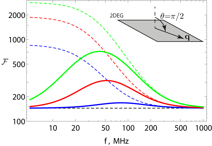
Figure 1: (Color online) The total enhancement factor $\mathcal{F}=\tau^{(0)}_{ph}/\tau_{ph}$ at $\theta=\pi/2$ of ultrasound attenuation in the 2D semiconductor InSb. The parameters taken are $n=10^{11}cm^{-2}$, $p_{F}l=50$, $\Delta_{SO}=0.1meV$ and magnetic fields are $3\,\mathrm{T}$ (blue), $5\,\mathrm{T}$ (red) and $7\,\mathrm{T}$ (green). Dashed curves represent the result in the absence of SO relaxation, $\Delta_{SO}=0$. The black dashed curve gives the enhancement $\mathcal{F}_{C}$ by incomplete screening.

In conclusion, we demonstrated an existence of a general relaxation mechanism that leads to enhancement of both the e-ph cooling power and the phonon decay rate. In particular, it may lead to a strong enhancement of the cooling power in disordered conductors in the external magnetic field or in disordered ferromagnetic metals.

We are grateful to S. Dorozhkin, M. Gershenson, J. Pekola, M. Reznikov and K. Tikhonov for useful discussions. The research done by M.V.F. and A.V.S was supported by the RFBR grant # 10-02-00554. A.V.S. also acknowledges support from Dynasty foundation.

Supplementary Material

I I. Hamiltonian

We consider an electron system with several spectral branches (which are labeled by $i\in(1,N)$ ). Interaction between electrons is considered in the direct (density-density) channel only, and will be treated within the random phase approximation (RPA). Electrons also scatter off local impurities, and we assume this scattering to be identical for all spectral branches, $U_{imp,i}({\bf r})=U_{imp}({\bf r})$. While treating electron-phonon inelastic processes, it is convenient to work in the co-moving frame of reference (CFR), where the effective Hamiltonian acquires the following form s_schmid ; s_reyzer ; s_kravtsov_yudson in the momentum representation:

$$H=H_{e0}+H_{e-e}+H_{e-ph},$$ (S17)

$$H_{e0}=\sum_{{\bf p},i}\xi_{i}({\bf p})\overline{\psi}_{{\bf p},i}\psi_{{\bf p},i}+\sum_{{\bf p},{\bf p}^{\prime},i}U_{imp}({\bf p}^{\prime}-{\bf p})\overline{\psi}_{{\bf p},i}\psi_{{\bf p}^{\prime},i},$$

$$H_{e-e}=\frac{1}{2}\sum_{{\bf q}}V_{0}({\bf q})n_{{\bf q}}n_{-{\bf q}},$$

$$H_{e-ph}=\sum_{{\bf q},i}\Gamma_{i}(\,{\rm{div}\bf{u}})_{{\bf q}}n_{-{\bf q},i},$$

where $U_{imp}({\bf r})$ is disorder potential, $V_{0}(q)$ is a bare Coulomb interaction attenuated by the background dielectric constant $\varepsilon$ which could be additionally screened by a metallic gate; $n_{{\bf q},i}=\sum_{{\bf p}}\overline{\psi}_{{\bf p}+{\bf q},i}\psi_{{\bf p},i}$ and $n_{{\bf q}}=\sum_{i}n_{{\bf q},i}$ are the i-th branch partial- and total densities, respectively. $\Gamma_{i}$ and $(\,{\rm{div}\bf{u}})_{{\bf q}}=i{\bf q}\cdot{\bf u}$ are the e-ph interaction constant averaged over the Fermi surface and the divergence of ionic displacement field ${\bf u}$. The Hamiltonian (S17) contains no inter-branch scattering. We assume these processes to be much weaker than the intra-branch scattering and discuss their role later on in Sec.III C.

For convenience, we present an explicit derivation of Hamiltonian in CFR.

I.1 Hamiltonian in LFR

In LFR electron-phonon interaction is mediated via two processes s_kravtsov_yudson . First, electron-phonon-ion, when phonons disturb positive ionic background density, $n_{ion}({\bf u})=n_{ion}(1-\,{\rm{div}\bf{u}})$. Second, when phonons displace impurities, ${\bf r}_{imp}({\bf u})\rightarrow{\bf r}_{imp}+{\bf u}({\bf r}_{imp})$, and thus affect random potential $U({\bf r})\rightarrow U({\bf r})-\nabla_{\alpha}(u_{\alpha}({\bf r})U({\bf r}))$:

$$H^{LFR}=H_{K}+H_{U}+H_{e-e}+H_{e-ph}^{LFR},$$ (S18)

$$H_{K}=\sum_{{\bf p},i}\xi_{i}({\bf p})\overline{\psi}_{{\bf p},i}\psi_{{\bf p},i},$$

$$H_{U}=\sum_{{\bf p},{\bf p}^{\prime},i}U_{imp}({\bf p}^{\prime}-{\bf p})\overline{\psi}_{{\bf p},i}\psi_{{\bf p}^{\prime},i},$$

$$H_{e-e}=\frac{1}{2}\sum_{{\bf q}}V_{0}({\bf q})n_{{\bf q}}n_{-{\bf q}},$$

$$H_{e-ph}^{LFR}=H_{e-ph-ion}^{LFR}+H_{e-ph-imp}^{LFR},$$

$$H_{e-ph-ion}^{LFR}=\sum_{{\bf q}}\left[(n_{ion}\,{\rm{div}\bf{u}})_{{\bf q}}V_{0}(q)\right]n_{-{\bf q}}$$ (S19)

$$=\sum\limits_{{\bf p},{\bf q},i}n_{ion}V_{0}(q)(i{\bf q}\cdot{\bf u}_{{\bf q}})\overline{\psi}_{{\bf p}+{\bf q},i}\psi_{{\bf p},i},$$

$$H_{e-ph-imp}^{LFR}=\sum_{{\bf q}}\left[\left(-\nabla_{\alpha}\left[u_{\alpha}U_{imp}({\bf r})\right]\right)_{{\bf q}}\right]n_{-{\bf q}}$$ (S20)

$$=\sum\limits_{{\bf p},{\bf q},i}U_{imp}({\bf p}^{\prime}-{\bf p})\left(-i({\bf p}^{\prime}+{\bf q}-{\bf p})\cdot{\bf u}_{{\bf q}}\right)\overline{\psi}_{{\bf p}^{\prime}+{\bf q},i}\psi_{{\bf p},i},$$

where $H_{K}$ and $H_{U}$ stand for kinetic and (unaltered) random potential energies respectively. Usually, this Hamiltonian is used under assumption of static screening in RPA approximation, when $V_{0}(q)\rightarrow V(q)=(\sum_{i}\nu_{i})^{-1}$, while electro-neutrality in equilibrium implies that $n_{ion}=\sum_{j}(n_{j})_{eq}=\sum_{j}\nu_{j}(p_{F}v_{F}/d)_{j}$.

I.2 Canonical transformation

As Tsuneto has shown s_tsuneto , transformation to a CFR in linear approximation in ${\bf u}$ is equivalent to a canonical transformation ${\widehat{U}}$:

$$\psi\rightarrow{\widehat{U}}\psi,\quad\psi={\widehat{U}}^{-1}\psi^{\prime}$$ (S21)

$${\widehat{U}}=\left(1+\frac{1}{2}\left\{u_{\alpha},\nabla_{\alpha}\right\}\right)=\left(1+\frac{1}{2}\,{\rm{div}\bf{u}}+{\bf u}\cdot\boldsymbol{\nabla}\right)$$

$$=\left(1+i{\bf u}_{{\bf q}}\cdot({\bf p}+{\bf q}/2)\right).$$ (S22)

This transformation alters the Hamiltonian , generating new terms linear in displacement ${\bf u}$ from $H_{K}$, $H_{U}$ and $H_{e-e}$. $H_{e-ph}^{LFR}$ obviously remains unaltered as it is already linear in ${\bf u}$. However, there is also a special term that arises from the left hand side of Schroedinger equation or, equivalently, from the time derivative in action.

I.2.1 Time derivative in LHS of Schroedinger equation

Time derivative in LHS of Schroedinger equation (primes are omitted for brevity) generates the term

$$i\overline{\psi}\partial_{t}\psi\rightarrow$$ (S23)

$$i\left(1-\frac{1}{2}\,{\rm{div}\bf{u}}-i{\bf u}\cdot{\bf\partial}\right)\overline{\psi}\partial_{t}\left(1-\frac{1}{2}\,{\rm{div}\bf{u}}-i{\bf u}\cdot{\bf\partial}\right)\psi$$

$$=i\overline{\psi}\partial_{t}\psi-i\overline{\psi}\left(\frac{1}{2}{\rm div}\dot{{\bf u}}+i\dot{{\bf u}}\cdot{\bf\partial}\right)\psi$$

$$H_{e-ph,LHS}^{CFR}=\sum_{{\bf p},{\bf q}i}\left(\dot{{\bf u}}_{{\bf q}}\cdot{\bf p}\right)\overline{\psi}_{{\bf p}+{\bf q},i}\psi_{{\bf p}-{\bf q},i}$$ (S24)

$$=\sum_{{\bf p},\varepsilon,\omega,{\bf q},i}\left(-i\omega{\bf u}_{\omega,{\bf q}}\cdot{\bf p}\right)\overline{\psi}_{{\bf p}+{\bf q}/2,\varepsilon+\omega,i}\psi_{{\bf p}-{\bf q}/2,\varepsilon,i}$$

I.2.2 Kinetic energy

$$H_{e-ph,1}^{CFR}=H_{K}\left[\overline{\left({\widehat{U}}^{-1}\psi\right)},{\widehat{U}}^{-1}\psi\right]-H_{K}\left[\overline{\psi},\psi\right]$$ (S25)

$$=-\sum_{{\bf p},{\bf q},i}\overline{\psi}_{i}\left[\left(\xi_{i}({\bf p}+{\bf q}/2)-\xi_{i}({\bf p}-{\bf q}/2)\right)i{\bf p}\cdot{\bf u}\right]\psi_{i}$$

$$=-\sum_{{\bf p},{\bf q},i}\overline{\psi}_{{\bf p}+{\bf q}/2,i}(i{\bf v}_{i}\cdot{\bf q})({\bf p}\cdot{\bf u}_{{\bf q}})\psi_{{\bf p}-{\bf q}/2,i}$$ (S26)

I.2.3 Random potential

$$H_{e-ph,2}^{CFR}=H_{U}\left[\overline{\left({\widehat{U}}^{-1}\psi\right)},{\widehat{U}}^{-1}\psi\right]-H_{U}\left[\overline{\psi},\psi\right]$$ (S27)

$$=-\sum_{{\bf p},{\bf p}^{\prime},{\bf q}i}U_{imp}({\bf p}^{\prime}-{\bf p})\left[i{\bf u}_{{\bf q}}\cdot({\bf p}-{\bf p}^{\prime})\right]\overline{\psi}_{{\bf p}^{\prime}+{\bf q}/2,i}\psi_{{\bf p}-{\bf q}/2,i}$$

I.2.4 Electron-electron interactions

Electron-electron interaction term is convenient to be analyzed in real space. Electron density is transformed under canonical transformation as

$$n_{i}({\bf r})=\overline{\psi}_{i}({\bf r})\psi_{i}({\bf r})\rightarrow\overline{\left({\widehat{U}}^{-1}\psi\right)}_{i}({\bf r})\left({\widehat{U}}^{-1}\psi\right)_{i}({\bf r}),$$

$$n_{i}({\bf r})\rightarrow n_{i}({\bf r})+\partial_{\alpha}(u_{\alpha}({\bf r})n_{i}({\bf r})).$$ (S28)

The contribution to electron-phonon interaction itself is

$$H_{e-ph,3}^{CFR}=H_{e-e}\left[\overline{\left({\widehat{U}}^{-1}\psi\right)},{\widehat{U}}^{-1}\psi\right]-H_{e-e}\left[\overline{\psi},\psi\right]$$

$$=-\sum\limits_{{\bf r},{\bf r}^{\prime}}u_{\alpha}({\bf r})\partial_{\alpha}V({\bf r}-{\bf r}^{\prime})n({\bf r})n({\bf r}^{\prime})$$ (S29)

$$=\sum\limits_{{\bf p},{\bf p}^{\prime},{\bf Q},{\bf q},i,j}iu_{{\bf q},\alpha}Q_{\alpha}V_{0}({\bf Q})\overline{\psi}_{{\bf p}+{\bf Q}+{\bf q},i}\overline{\psi}_{{\bf p}^{\prime},j}\psi_{{\bf p}^{\prime}+{\bf Q},j}\psi_{{\bf p},i}.$$

I.3 Full expression for e-ph interaction in CFR

Electron-phonon interaction in CFR after canonical transformation is the sum of all parts

$$H_{e-ph}^{CFR}=H_{e-ph}^{LFR}+H_{e-ph,LHS}^{CFR}+\sum_{i}H_{e-ph,i}^{CFR}.$$ (S30)

Two major facts should be emphasized.

First, electron-phonon-impurity interaction almost cancels out by the part arising from random potential energy:

$$H_{e-ph-imp}^{LFR}+H_{e-ph,2}^{CFR}$$ (S31)

$$=-\sum\limits_{{\bf p},{\bf q},i}U_{imp}({\bf p}^{\prime}-{\bf p})\left(i{\bf q}\cdot{\bf u}_{{\bf q}}\right)\overline{\psi}_{{\bf p}^{\prime}+{\bf q},i}\psi_{{\bf p},i}$$

This cancellation reflects the fact that canonical transformation returns impurities to equilibrium position, while the remaining part is present due to non-uniformity of the transformation.

Second, in Hartree-Fock approximation electron-phonon-ion term is canceled out by the one arising from electron-electron interactions s_schmid :

$$\left(H_{e-ph,3}^{CFR}\right)_{HF}=$$ (S32)

$$\sum\limits_{{\bf p},{\bf p}^{\prime},{\bf Q},{\bf q},i,j}iu_{{\bf q},\alpha}Q_{\alpha}V_{0}({\bf Q})\left\langle\overline{\psi}_{{\bf p}+{\bf Q}+{\bf q},i}\psi_{{\bf p},i}\right\rangle\overline{\psi}_{{\bf p}^{\prime},j}\psi_{{\bf p}^{\prime}+{\bf Q},j}$$

$$=-\sum\limits_{{\bf p},{\bf p}^{\prime}{\bf q},j}iu_{{\bf q},\alpha}q_{\alpha}V_{0}(q)(n_{el})_{eq}\overline{\psi}_{{\bf p}^{\prime},j}\psi_{{\bf p}^{\prime}-{\bf q},j}$$

$$=-H_{e-ph-ion}^{LFR}$$ (S33)

Thus, electron-phonon interaction in CFR is of the form

$$\left(H_{e-ph}^{CFR}\right)_{HF}=-\sum_{{\bf p},{\bf q},i}\left(\dot{{\bf u}}_{{\bf q}}\cdot{\bf p}\right)\overline{\psi}_{{\bf p}+{\bf q}/2,i}\psi_{{\bf p}-{\bf q}/2,i}$$

$$-\sum_{{\bf p},{\bf q},i}\overline{\psi}_{{\bf p}+{\bf q}/2,i}(i{\bf v}_{i}\cdot{\bf q})({\bf p}\cdot{\bf u}_{{\bf q}})\psi_{{\bf p}-{\bf q}/2,i}$$ (S34)

$$-\sum\limits_{{\bf p},{\bf q},i}U_{imp}({\bf p}^{\prime}-{\bf p})\left(i{\bf q}\cdot{\bf u}_{{\bf q}}\right)\overline{\psi}_{{\bf p}^{\prime}+{\bf q},i}\psi_{{\bf p},i}$$

For the problem in question, effects arising from the first term are small in adiabatic parameter $s/v_{F}$, while possible effects arising from the third one are small in inverse conductance $(p_{F}l)^{-1}$. Thus, they may be safely omitted.

Finally, there is screening by electron-electron interactions $H_{e-e}$. In this paper we start with bare electron-phonon vertices $H_{e-ph}^{CFR}$ and take into account screening explicitly (for example, we sum up diagrammatic ladders given on the Fig.S2). In a number of papers a bit different formulation of the problem is used; namely, it is assumed from the very beginning that full screening of Coulomb interaction takes place. Within such an approach electron-electron interaction does not appear in the explicit form in the calculations; instead, an additional term that describes the above screening is added into the electron-phonon vertex. In Eq.(36) below we present, for the sake of completeness, the corresponding form of the electron-phonon interaction in the co-moving frame (with first and third terms of (S35) omitted)

$$\left(H_{e-ph}^{CFR}\right)_{scr}=$$ (S35)

$$-\sum_{{\bf p},{\bf q},i}\overline{\psi}_{{\bf p}+{\bf q}/2,i}(i{\bf v}_{i}\cdot{\bf q})({\bf p}\cdot{\bf u}_{{\bf q}})\psi_{{\bf p}-{\bf q}/2,i}$$

$$+\sum_{{\bf p},{\bf q},i}\overline{\psi}_{{\bf p}+{\bf q}/2,i}\left(V_{RPA}\sum\limits_{j}\nu_{j}\left(\frac{p_{F}v_{F}}{d}\right)_{j}\,{\rm{div}\bf{u}}\right)\psi_{{\bf p}-{\bf q}/2,i},$$

where we assume static screening in RPA approximation, $V_{RPA}=(\sum_{j}\nu_{j})^{-1}$.

II II. Derivation of the phonon kinetic equation

Here we derive the phonon quantum kinetic equation via the Keldysh diagrammatic technique (see Ref.s_Kamenev-Levchenko, for details). For simplicity, we consider only the longitudinal phonons; the transverse phonons may be analyzed in a similar way. The Green’s functions are matrices in the Keldysh space:

$${\widehat{D}}=\left(\begin{array}[]{cc}D^{K}&D^{R}\\ D^{A}&0\end{array}\right),$$ (S38)

$${\widehat{D}}_{0}^{-1}=\left(\begin{array}[]{cc}0&(D_{0}^{A})^{-1}\\ (D_{0}^{R})^{-1}&0\end{array}\right),\,{\widehat{\Sigma}}=\left(\begin{array}[]{cc}0&\Sigma^{A}\\ \Sigma^{R}&\Sigma^{K}\end{array}\right),$$ (S43)

where $D_{0}$ and $D$ are the bare and exact phonon Green’s functions, respectively and $\Sigma$ is the self-energy part. The Keldysh component $(\dots)^{K}$ may be parametrized as

$$D^{K}=D^{R}\circ F-F\circ D^{A}$$ (S44)

where $F$ is related to the phonon distribution function; in equilibrium $F=\coth(\omega/2T)$. The sign $\circ$ means the convolution in the time domain. A bare retarded(advanced) phonon Green’s function is

$$D_{0}^{R(A)}(\omega,q)=\frac{1}{\hbar^{2}\rho_{m}}\frac{1}{(\omega\pm i0)^{2}-v_{s}^{2}q^{2}},$$ (S45)

where $\rho_{m}$ is the mass density. To derive the kinetic equation one employs the Dyson equation for the matrix Green functions which together with Eq.(S44)results in:

$$({\widehat{D}}_{0}^{-1}-{\widehat{\Sigma}}){\widehat{D}}=1,\quad\Rightarrow$$ (S46)

$$\Rightarrow \left[D_{0}^{-1},F\right]=\Sigma^{K}-\Sigma^{R}\circ F-F\circ\Sigma^{A}.$$ (S47)

According to Eq.(S45) $D_{0}^{-1}$ contains the second derivative with respect to the corresponding time argument of $F\equiv F(t_{1},t_{2})$. Then the commutator in Eq.(S47) reduces to the first derivative $\partial_{t}$ with respect to the ”slow” combination $t=t_{1}+t_{2}$ multiplied by the Fourier transform $-i\omega$ of the derivative with respect to the ”fast” combination $t_{1}-t_{2}$. Averaging over the whole volume of the sample, one finds

$$2i\rho_{m}\omega\partial_{t}F=\Sigma^{K}-\Sigma^{R}\circ F-F\circ\Sigma^{A}.$$ (S48)

In this equation we assume $F(t_{1},t_{2})\rightarrow F(\omega;t)$. We also omit the terms describing the external source that pumps energy into electronic system.

A common action of the source term and the e-ph energy relaxation leads to a stationary energy distribution of both electrons and phonons. If the e-ph energy relaxation is much slower than the electron-electron one, a quasi-equilibrium situation with two temperatures $T_{el},\,T_{ph}$ is realized s_comment . In this case the phonon distribution function is $F(\omega,T_{ph})=\coth(\omega/2T_{ph})$ while $\Sigma^{K}$ is a quasi-equilibrium quantity. If in addition a weak e-ph interaction is assumed, electron-phonon interaction enters only trivially as the square of the e-ph matrix element in the Keldysh self-energy part $\Sigma^{K}$. In this approximation $\Sigma^{K}$ depends only on the electron temperature, $\Sigma^{K}=F(\omega,T_{el})(\Sigma^{R}-\Sigma^{A})$,

$$2i\rho_{m}\omega\partial_{t}F(\omega,T_{ph}(t))=\left[F\cdot(\Sigma^{R}-\Sigma^{A})\right](\omega,q,T_{el})$$

$$-\left[F\cdot(\Sigma^{R}-\Sigma^{A})\right](\omega,q,T_{ph}).$$ (S49)

Since the phonon decay rate is relatively low, $\tau_{ph}^{-1}\ll\omega$, phonons are well-defined quasiparticles and the quasiparticle distribution function is sharply peaked around the phonon ”mass-shell” $\omega=sq$. Thus, the quantities entering in the R.H.S. of Eq.(S49) should be taken at $\omega=sq$, see Ref. s_Kamenev-Levchenko . For convenience we introduce a standard phonon distribution function $B(\omega)=(1/2)(F(\omega)-1)$ and define a decay rate $\tau_{ph}^{-1}$:

$$\tau_{ph}^{-1}(\omega,T_{el})=\frac{1}{\rho_{m}\omega}{\rm Im\,}\Sigma^{R}(\omega,q,T_{el})|_{\omega=sq},$$ (S50)

$$\partial_{t}B(\omega,T_{ph}(t))=\frac{B(\omega,T_{el})-B(\omega,T_{ph})}{\tau_{ph}(\omega,T_{el})}.$$ (S51)

In order to obtain an electron-phonon heat flow, we have to multiply Eq.(S51) by both phonon density of states $\nu_{ph}(\omega)=\omega^{2}/2\pi^{2}v_{s}^{3}$ and by energy, and integrate over $\omega$:

$$\mathcal{J}=\int\limits_{0}^{\infty}d\omega\,\nu_{ph}(\omega)\,\omega\,\partial_{t}\,B(\omega,T_{ph}(t))$$ (S52)

$$=\int\limits_{0}^{\infty}d\omega\,\nu_{ph}(\omega)\,\frac{\omega}{\tau_{ph}(\omega,T_{el})}\left[B(\omega,T_{el})-B(\omega,T_{ph})\right]$$

The incoming and outgoing energy flows may be defined as follows:

$$\mathcal{J}(T_{el},T_{ph})=J_{+}(T_{el})-J_{-}(T_{ph},T_{el}),$$ (S53)

$$J_{+}(T_{el})=\int\limits_{0}^{\infty}d\omega\,\nu_{ph}(\omega)\,\frac{\omega}{\tau_{ph}(\omega,T_{el})}B(\omega,T_{el}),$$

$$J_{-}(T_{ph},T_{el})=\int\limits_{0}^{\infty}d\omega\,\nu_{ph}(\omega)\,\frac{\omega}{\tau_{ph}(\omega,T_{el})}B(\omega,T_{ph}),$$

In general, $J_{-}$ depends on both $T_{el}$ and $T_{ph}$ due to the effect of electron-electron interactions on the decay rate $\tau_{ph}^{-1}$, see Eq.(S50). However such an effect is absent within the RPA approximation for charge screening which we use here. Thus our result for the phonon lifetime does not depend on temperature explicitly, $\tau_{ph}=\tau_{ph}(\omega)$. In this case the expressions for heat flows are simplified and $J_{-}$ becomes a function of the phonon temperature $T_{ph}$ only.

The electronic temperature relaxation rate $\tau_{E}^{-1}$ can be obtained from the expression for the heat flow $\mathcal{J}_{e-ph}$. Each phonon branch contributes as

$$\tau_{E,\alpha}^{-1}=\frac{1}{C_{e}}\left.\frac{\partial\mathcal{J}_{e-ph,\alpha}}{\partial T_{el}}\right|_{T_{ph}=T_{el}}$$ (S54)

$$=\frac{1}{4C_{e}T^{2}}\int\limits_{0}^{\infty}d\omega\frac{\omega^{2}\nu_{ph}(\omega)}{\sinh^{2}(\omega/2T)}\tau_{ph,\alpha}^{-1}(\omega,T)$$

where $C_{e}\propto\nu T$ is the electronic specific heat. The full rate is then $\tau_{E,f}^{-1}=\tau_{E,l}^{-1}+(d_{ph}-1)\tau_{E,tr}^{-1}$, where $(d_{ph}-1)$ is the number of transverse phonon polarizations. Electrons are characterized by the quasi-equilibrium distribution function if their intrinsic inelastic scattering time $\tau_{ee}$ is much shorter than the temperature relaxation time $\tau_{E}$ due to interaction with phonons.

Finally, let us mention that in 2D electron systems the phonon decay rate $\tau_{ph}({\bf q})$ depends on the angle $\theta$ between the phonon momentum ${\bf q}$ and the direction normal to the plane of the 2DEG. Thus, in the equations like (S52,S53,S54) an angle-averaged decay rate should be used:

$$\left<\tau_{ph}^{-1}\right>_{\theta}(\omega)=\frac{1}{2}\int_{0}^{\pi}(\sin\theta d\theta)\,\tau^{-1}_{ph}(\omega,\theta)$$ (S55)

III III. Diagrammatic derivation

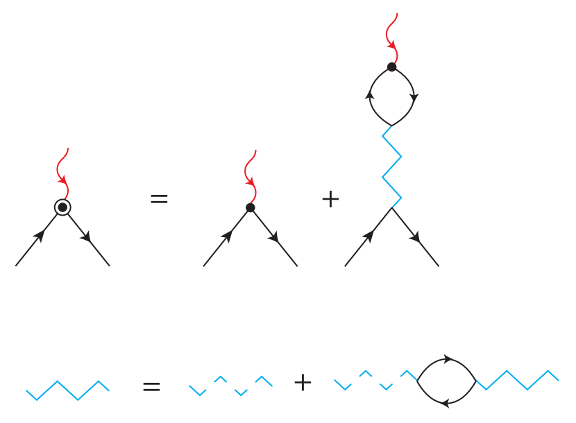
Figure S2: Bare and screened e-ph vertices. Black, curvy red and dashed blue zig-zag lines are electron, phonon and Coulomb interaction propagators respectively. Bold zig-zag lines stand for statically screened Coulomb interaction (with screening by empty electron bubbles only).

We present here the derivation of some of our results in the standard diagrammatic form, as it was done in the most papers on this subject s_schmid ; s_reyzer ; s_kravtsov_yudson .

The bare electron-phonon vertex corresponding to the Hamiltonian (S17) is of tensor structure in the space of electron species:

$${\widehat{\Gamma}}_{bare}=\left(\begin{array}[]{ccc}\Gamma_{1}&&\\ &\ddots&\\ &&\Gamma_{N}\end{array}\right).$$ (S56)

The diagonal structure of (S56) corresponds to our assumption about the absence of inter-branch mixing. Now one should take into account static Coulomb screening, which generates scalar counter-term

$${\widehat{\Gamma}}_{C}=-\frac{\sum_{i}\Gamma_{i}\nu_{i}}{V_{0}^{-1}(q)+\sum_{i}\nu_{i}}{\widehat{1}}$$ (S57)

The full screened vertex is then a sum ${\widehat{\Gamma}}_{full}={\widehat{\Gamma}}_{bare}+{\widehat{\Gamma}}_{C}$. The structure of these vertices is presented in Fig.S2. The deformation potentials $\Gamma_{i}$ averaged over FS are usually approximated as s_schmid

$$\Gamma_{i}=\left[\left.\left(\Gamma_{bs}({\bf p})\right)\right|_{FS}-p_{F}v_{F}/d_{e}\right]_{i}$$ (S58)

where $\Gamma_{bs}$ represents the lattice-induced deformation potential under the lattice strain and $p_{F}v_{F}/d_{e}$ represents the averaged electron liquid stress tensor. We will consider the simplest model where the lattice contribution is uniform in momentum space $\Gamma_{bs}({\bf p})=\Gamma_{bs}$ and thus is reduced to the shift of electron band  (see however Ref. s_comment2 ).

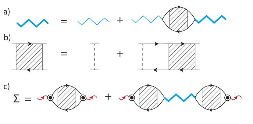
Figure S3: a) Dynamically screened Coulomb interaction, where diffusion is taken into account. Namely, an impurity ladder is summed up  b) The impurity ladder. Here black dashed line represents impurity correlator $\left\langle U({\bf r})U({\bf r}^{\prime})\right\rangle$. c) Diagrams contributing to phonon self energy. This figure encompasses the very general case with arbitrary number of electron types and arbitrary Coulomb interaction strength. Inside the electron bubbles summation goes over all electron branches

In order to evaluate the decay rate and the electron cooling rate we need to calculate the imaginary part of the phonon self energy $\Sigma$. It is represented by the diagrams shown in a Fig.S3. The second diagram is important when the screening is essentially dynamic. Below we demonstrate few particular examples how the diagrammatic description works.

III.1 A. Imperfect screening

In this Subsection we consider the case of identical spectral branches, but assuming now that screening is incomplete and electron density variations are allowed. Then the full e-ph vertex given by the sum of Eq.(S56) and Eq.(S57) is diagonal:

$${\widehat{\Gamma}}_{s}=\frac{\Gamma}{1+N_{f}\nu V_{0}(q)}$$ (S59)

where $N_{f}$ is a number of identical electron branches. Typically it is equal to $N_{f}=2N_{v}$ where $N_{v}$ is the number of identical valleys in a semiconductor. For example, $N_{v}=6$ for a bulk silicon or $N_{v}=2$ for graphene. The first diagram from the Fig.S3c thus gives

$$\Sigma_{1}=\left(\frac{\Gamma}{1+\nu N_{f}V_{0}(q)}\right)^{2}q^{2}N_{f}\nu\frac{i\omega}{-i\omega+Dq^{2}}$$ (S60)

The second diagram turns out to be crucial for a dynamical screening regime, when $\omega\geq Dq^{2}$:

$$\Sigma_{2}=\left(\frac{\Gamma q}{1+\nu N_{f}V_{0}(q)}\right)^{2}\left(N_{f}\nu\frac{i\omega}{-i\omega+Dq^{2}}\right)^{2}$$ (S61)

$$\times\left(-\frac{1}{V_{0}^{-1}(q)+N_{f}\nu Dq^{2}/(-i\omega+Dq^{2})}\right)$$

Summing up these contributions we obtain $\Sigma=\Sigma_{1}+\Sigma_{2}$:

$$\Sigma=\frac{\Gamma^{2}q^{2}}{1+N_{f}\nu V_{0}(q)}\times$$ (S62)

$$\times N_{f}\nu\left(\frac{i\omega(i\omega+Dq^{2}+(N_{f}\nu V_{0}(q)Dq^{2})}{\omega^{2}+(Dq^{2})^{2}(1+N_{f}\nu V_{0}(q))^{2}}\right).$$

The phonon decay rate is determined by the imaginary part of $\Sigma$:

$$\tau_{ph,ML}^{-1}=\frac{\Gamma^{2}}{\rho_{m}}\frac{N_{f}\nu Dq^{2}}{v_{s}^{2}+(Dq)^{2}(1+N_{f}\nu V_{0}(q))^{2}},\\$$ (S63)

and the corresponding enhancement factor is

$$\mathcal{F}_{C}(q)=1+\frac{1}{c_{l}}\frac{(\Gamma/p_{F}v_{F})^{2}}{(v_{s}/v_{F})^{2}+d_{e}^{-2}(q^{2}l^{2})(1+N_{f}\nu V_{0}(q))^{2}}$$ (S64)

These results coincide with the ones in the main text for $N_{f}=2$. Thus, we have shown equivalence of the approach using macroscopic kinetic equation and diagrammatic technique.

III.2 B. Several spectral branches

Now we switch to the situation of complete screening of Coulomb interaction, so the electro-neutrality condition is obeyed exactly. In such a case the difference in the coupling constants $\Gamma_{i}$ corresponding to different electron branches is crucial. We consider here the simplest case of two spectral branches. Then the full screened e-ph vertex given by the sum of Eqs.(S56) and (S57) is traceless:

$${\widehat{\Gamma}}_{s}=\left(\begin{array}[]{cc}\frac{\Gamma_{1}-\Gamma_{2}}{2}&\\ &-\frac{\Gamma_{1}-\Gamma_{2}}{2}\end{array}\right).$$ (S65)

The diagrams shown in Fig.S3c give

$$\Sigma=2\times\left(\frac{\Gamma_{1}-\Gamma_{2}}{2}\right)^{2}q^{2}\nu\frac{i\omega}{-i\omega+Dq^{2}}$$ (S66)

Thus, the phonon decay rate due to the Mandelstam-Leontovich mechanism is

$$\tau_{ph}^{-1}=\frac{1}{\rho_{m}\omega}\left[{\rm Im\,}\Sigma(\omega,q)\right]_{\omega=sq}$$ (S67)

$$=\frac{(\Gamma_{1}-\Gamma_{2})^{2}}{2\rho_{m}}\frac{\nu Dq^{2}}{v_{s}^{2}+(Dq)^{2}},$$

and the total decay rate is enhanced (with respect to the classical Pippard result) by the factor

$$\mathcal{F}(q)=1+\frac{1}{4c_{l}}\left(\frac{\Gamma_{1}-\Gamma_{2}}{p_{F}v_{F}}\right)^{2}\frac{v_{F}^{2}}{v_{s}^{2}+(Dq)^{2}}$$ (S68)

If the asymmetry in spectral branches arise due to the Zeeman splitting, then $\Gamma_{1}-\Gamma_{2}=(2/d_{e})g\mu_{B}H$:

$$\mathcal{F}_{H}(q,h)=1+\frac{1}{d_{e}^{2}c_{l}}\frac{v_{F}^{2}h^{2}}{v_{s}^{2}+(Dq)^{2}}$$ (S69)

where $h=g\mu_{B}H/2\varepsilon_{F}\ll 1$ is dimensionless magnetic field (we neglect here $h$-dependencies of other parameters, like difference $D_{1}\neq D_{2}$, which is negligible at $h\ll 1$).

Note that the effect is absent in zero magnetic field, as the time-reversal symmetry does not allow spin density fluctuations to be excited by phonons.

III.3 C. Spin-orbit coupling and interbranch scattering

In this Subsection we revisit the case of the two inequivalent branches of electron spectrum and consider the (previously neglected) role of the interbranch scattering, using the Zeeman-splitting as an example. Qualitatively, the spin-flip scattering with a rate $\tau_{r}^{-1}$ leads to non-conservation of the total spin and thus limits the magnitude of any effect which is related to slow spin diffusion. Formally it is described by the modification of the spin diffusion propagator:

$$\frac{Dq^{2}}{-i\omega+Dq^{2}}\Rightarrow\frac{Dq^{2}}{-i\omega+Dq^{2}+1/2\tau_{r}}$$ (S70)

which leads to the replacement of Eq.(S69) by

$$\mathcal{F}_{H}(q,h)=1+\frac{1}{d_{e}^{2}c_{l}}\frac{v_{F}^{2}q^{2}h^{2}}{\omega^{2}+(Dq^{2}+1/2\tau_{r})^{2}}.$$ (S71)

Below we calculate $\tau_{r}$ for the case of 2D electron gas with the Zeeman splitting induced by magnetic field applied in the 2DEG plane in the $x$-axis direction.

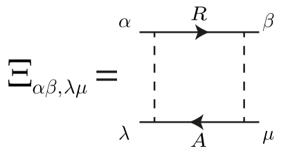
Figure S4: Diffuson self energy ${\widehat{\Xi}}$, $\mathcal{{\widehat{D}}}=(1/2\pi\nu\tau)(1-{\widehat{\Xi}})^{-1}$. Capital letters $A$ and $R$ stand for advanced and retarded electron Green functions respectively.

We assume a relatively weak spin-orbit (SO) interaction leading to the spin-orbit band splitting $\Delta_{SO}\ll\Delta_{H}=g\mu_{B}H$. For definiteness we consider the Rashba-type SO coupling with the spin-dependent part of the Hamiltonian being equal to

$$H_{H+SO}=-\frac{\Delta_{H}}{2}{\widehat{\sigma}}_{x}+\frac{\Delta_{SO}}{2}(\sigma_{x}n_{y}-\sigma_{y}n_{x}),$$ (S72)

where ${\bf n}={\bf p}/|{\bf p}|$ is a unit vector in the direction of momentum. The elastic scattering time turns out to be equal for both quasiparticle branches(in the absence of electron-hole asymmetry):

$${\widehat{G}}^{R}(\varepsilon,{\bf p})=\sum\limits_{\pm}\frac{{\widehat{P}}_{\pm}}{\varepsilon-\xi\mp\Delta({\bf n})/2+i/2\tau},$$ (S73)

$${\widehat{P}}_{\pm}=\frac{1}{2}\left(1\pm\frac{\Delta_{H}\sigma_{x}-\Delta_{SO}(\sigma_{x}n_{y}-\sigma_{y}n_{x})}{\Delta({\bf n})}\right),$$ (S74)

$$\Delta({\bf n})=\sqrt{\Delta_{H}^{2}+\Delta_{SO}^{2}-2\Delta_{H}\Delta_{SO}n_{x}}.$$ (S75)

where ${\widehat{G}}^{R}$ is the retarded electron Green’s function. In order to find the relaxation rate, we evaluate the diffuson self energy for zero frequency and momentum ($\omega=0,\,{\bf q}=0$), Fig.S4:

$${\widehat{\Xi}}=\frac{1}{2\pi\nu\tau}\int\frac{d{\bf p}}{(2\pi)^{2}}{\widehat{G}}^{A}(0,{\bf p})\otimes{\widehat{G}}^{R}(0,{\bf p})$$ (S76)

A simple calculation in a manner similar to that of Ref.s_skvortsov, leads to the following result for the diffuson self energy at $q=\omega=0$:

$${\widehat{\Xi}}=\left(1-{\widehat{S}}_{x}^{2}\left[1-\frac{1}{1+\tau^{2}\Delta_{H}^{2}}\right]-\frac{i\tau\Delta_{H}}{1+\tau^{2}\Delta_{H}^{2}}{\widehat{S}}_{x}\right)-\frac{\Delta_{SO}^{2}}{2\Delta_{H}^{2}}\left(\frac{\tau^{2}\Delta_{H}^{2}}{1+\tau^{2}\Delta_{H}^{2}}{\widehat{S}}_{y}^{2}-\tau^{2}\Delta_{H}^{2}\frac{(3+\tau^{4}\Delta_{H}^{4})}{(1+\tau^{2}\Delta_{H}^{2})^{3}}{\widehat{S}}_{x}^{2}-\frac{4i\tau^{3}\Delta_{H}^{3}}{(1+\tau^{2}\Delta_{H}^{2})^{3}}{\widehat{S}}_{x}\right)$$ (S77)

with ${\bf{\widehat{S}}}=({\widehat{1}}\otimes\boldsymbol{{\widehat{\sigma}}}-\boldsymbol{{\widehat{\sigma}}}\otimes{\widehat{1}})/2$ being the total spin of electron-hole pair. We are interested in the $S_{x}=0$ subspace only as it hosts two eigenvalues of our interest. Naturally, the singlet mode($S=0$) corresponding to the charge density propagation remains unaffected, $\Xi_{S=0}=1$, while the triplet mode($S=1,S_{x}=0$) representing a spin density diffusion does decay:

$$\Xi_{S=1,S_{x}=0}=1-\frac{1}{2}\frac{\Delta_{SO}^{2}}{\Delta_{H}^{2}+\tau^{-2}}$$ (S78)

leading to the following result for the spin decay rate

$$\tau_{r}^{-1}\equiv\tau_{so}^{-1}=\frac{\Delta_{SO}^{2}}{\Delta_{H}^{2}+\tau^{-2}}\tau^{-1}\ll\tau^{-1}$$ (S79)

In the course of derivation of Eq.(S78) we used an identity $\langle S=1,S_{x}=0|{\widehat{S}}^{2}_{y}|S=1,S_{x}=0\rangle=1$. We emphasize that Eq.(S79) was derived for weak SO interaction, $\Delta_{SO}\ll\Delta_{H}$.

IV IV. Angular dependence of ultrasonic attenuation

We start here by the quasi-2D case when the thickness of a semiconductor film is much larger than the Fermi wavelength but still smaller than the phonon wavelength, $\lambda_{F}\ll b\ll\lambda_{ph}$. In this case electron diffusion is two-dimensional and only the component of phonon momentum parallel to the plane enters into the diffusion propagator where a replacement $Dq^{2}/(-i\omega+Dq^{2})\Rightarrow D{\bf q}_{\parallel}^{2}/(-i\omega+D{\bf q}_{\parallel}^{2})$ should be made. The result is that Eqs.(S69,S64) should be replaced by

$$\mathcal{F}_{C}(q)=1+\frac{c_{l}^{-1}(\Gamma/p_{F}v_{F})^{2}\sin^{2}\theta}{(v_{s}/v_{F})^{2}+(2/d_{e})^{2}g_{\Box}^{2}(e^{2}/\varepsilon\hbar v_{F})^{2}},$$ (S80)

$$\mathcal{F}_{H}(q)=1+\frac{1}{4c_{l}}\frac{v_{F}^{2}h^{2}\sin^{2}\theta}{v_{s}^{2}+(Dq)^{2}\sin^{4}\theta},$$ (S81)

where the last equation is given for relatively strong screening $\nu V_{0}(q)\gg 1$.

The true 2D case, however, should be discussed specially. While the result for the case of imperfect screening at $|\Gamma|\gg p_{F}v_{F}$ is identical to Eq.(S80), the magnetic-field induced effect (arising from the momentum-dependent part of the electron-phonon vertex) may behave differently.

For a sufficiently thin film electron motion in the direction perpendicular to the plane is fully quantized, thus the expression for electron-phonon vertex becomes

$$\Gamma_{1,2}=\Gamma_{bs}\,{\rm{div}\bf{u}}-\frac{1}{m}\langle p_{z}^{2}\rangle_{z}(iq_{z}u_{z})$$ (S82)

$$-\frac{p^{2}_{\parallel}}{2m}(iq_{x}u_{x}+iq_{y}u_{y})$$

$$=\left(\Gamma_{bs}-\frac{1}{m}\langle p_{z}^{2}\rangle_{z}\cos^{2}\theta-\frac{p^{2}_{\parallel}}{2m}\sin^{2}\theta\right)\,{\rm{div}\bf{u}},$$

where

$$\frac{p^{2}_{\parallel}}{2m}=\varepsilon_{F}\pm g\mu_{B}H-\frac{\langle p^{2}_{z}\rangle_{z}}{2m}$$ (S83)

with $\pm$ corresponding to the spin-up and spin-down electrons.

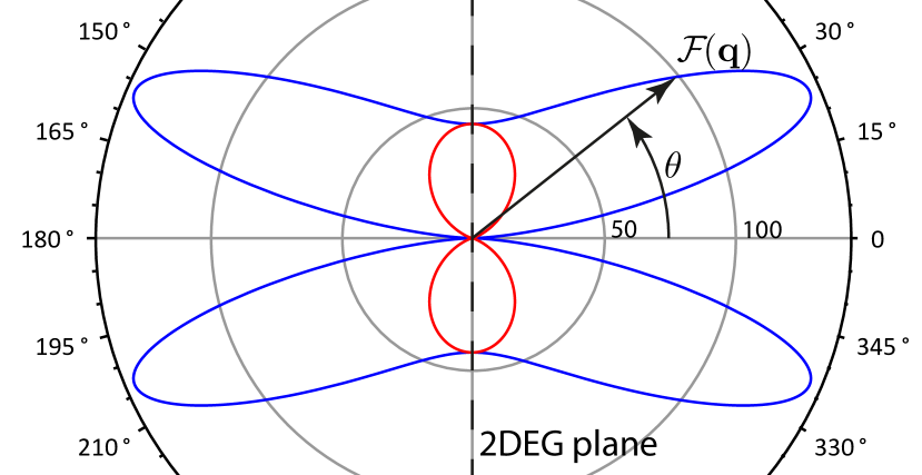
Figure S5: Angular dependence of ultrasonic attenuation for magnetic-field-controlled case, Eq.S86. Red and blue curves represent ($\gamma_{\parallel}=0,\gamma_{\perp}=0$) and ($\gamma_{\parallel}=0,\gamma_{\perp}=1$) respectively. Both plots are given for parameters of InSb sample from the main text at frequency $\omega=200\,\mathrm{MHz}$

Here we have taken an average $\langle\cdot\rangle_{z}$ over the ground state corresponding to the motion in the perpendicular direction and $p_{\parallel}$ is the momentum of an in-plane motion. We assume that the matrix element $\langle p^{2}_{z}\rangle_{z}$ does not depend on the spin degree of freedom as well as on the electron density. Thereby we disregard any possible orbital effects of magnetic field and consider the Zeeman interaction only which results in two different momenta $p_{\parallel,\uparrow}$ and $p_{\parallel,\downarrow}$ corresponding to the in-plane motion for the up and the down spin projections. The momentum-independent component of the vertex does not contribute to the magnetic-field-controlled relaxation under the condition of perfect screening (according to Eq.(S57) it is screened out completely). Eqs.(S68) explicitly implies that only asymmetric part of the vertex contributes:

$$\Gamma_{1}-\Gamma_{2}=g\mu_{B}H\sin^{2}\theta\,{\rm{div}\bf{u}}$$ (S84)

However, in real 2D electron systems, such as heterostructures, the lattice strain also affects momentum-dependent part of the quasiparticle spectrum. In other words, it alters electron effective mass. We limit ourselves to the particular case when

$$\delta m^{-1}=-m^{-1}(\gamma_{\perp}\cos^{2}\theta+\gamma_{\parallel}\sin^{2}\theta)\,{\rm{div}\bf{u}},$$ (S85)

$$\Gamma_{1}-\Gamma_{2}=g\mu_{B}H\times[(1+\gamma_{\parallel})\sin^{2}\theta+\gamma_{\perp}\cos^{2}\theta]\,{\rm{div}\bf{u}}.$$

Thus, the magnetic-field-controlled enhancement becomes equal to

$$\mathcal{F}_{H}(q,h)=1+$$ (S86)

$$\frac{v_{F}^{2}h^{2}\sin^{2}\theta}{v_{s}^{2}+(Dq)^{2}\sin^{4}\theta}[(1+\gamma_{\parallel})\sin^{2}\theta+\gamma_{\perp}\cos^{2}\theta]^{2}$$

The results (S80,S81,S86) show the angular dependence of ultrasonic attenuation which may exhibit a characteristic cross-like pattern exemplified in Fig.S5.

There are two additional issues which should be addressed to make the above analysis really quantitative: (i) in a general case the incident longitudinal(transverse) acoustic wave reflected off the free surface produces both longitudinal and transverse reflected waves, (ii) in the true 2D case diffusion modes could be generated by transverse phonons as well. However, these effects do not seem to lead to any qualitative change of our results and we will postpone the corresponding studies for the future.

V V. Electron-phonon heat flow

In this Subsection we use previously obtained results for the phonon decay rate, Eqs.(S80-S81), to derive an expression for the electron-phonon heat flow in a true 2D electron gas structure. We start by the spin density diffusion effects. At the lowest temperatures $T\ll T_{H}^{(1)}=\hbar v_{s}^{2}/D$, the enhancement does not depend on temperature and angle, being just a numerical factor:

$$J_{H}=g_{\Box}\frac{\pi^{3}p_{F}^{2}v_{F}^{2}h^{2}}{126\hbar^{6}\rho_{m}v_{s}^{7}}A_{1}T^{6},$$ (S87)

where $A_{1}=(48(1+\gamma_{\parallel})^{2}+16(1+\gamma_{\parallel})\gamma_{\perp}+6\gamma_{\perp}^{2})/105$ and $g_{\Box}=k_{F}l$ is the dimensionless conductance of the 2DEG. For higher temperatures, $T\gg T_{H}^{(1)}$, the enhancement factor behaves as $\mathcal{F}\propto T^{-2}$. However, the resulting expression for the e-ph heat flow depends significantly on the angular structure of the vertex

$$J_{H}=\frac{1}{g_{\Box}}\frac{\pi p_{F}^{4}h^{2}}{120\hbar^{6}\rho_{m}v_{s}^{3}}\left(A_{2}+\gamma_{\perp}^{2}\ln T/T_{H}^{(1)}\right)T^{4}$$

$$A_{2}=\frac{4}{3}(1+\gamma_{\parallel})(1+\gamma_{\parallel}+\gamma_{\perp})$$ (S88)

$$+\gamma_{\perp}^{2}\left(\frac{90}{\pi^{4}}\zeta^{\prime}(4)-\frac{5+6\gamma}{6}\right)$$

where $\zeta^{\prime}$ is the derivative of Riemann zeta function and $\gamma=0.577$ is the Euler’s constant respectively. If the normal strain does not alter electron mass ($\gamma_{\perp}=0$) the angular dependence $\mathcal{F}(q,\theta)$ does not lead to dominance of small $\theta$ in the corresponding integral. Then the heat flow is a pure power-law $J\propto T^{4}$. Otherwise, the shape of $\mathcal{F}(q,\theta)$ is rather peculiar (see Fig.S5) and an additional $\ln T$ factor appears due to the contribution of small angles $\theta_{H}\sim\sqrt{T_{H}^{(1)}/T}$. Note that the $T^{4}\ln T$ behavior is slower than $T^{6}$ and at temperatures

$$T>T_{H}^{(2)}=T_{H}^{(1)}\,\sqrt{1+\frac{h^{2}v_{F}^{2}}{v_{s}^{2}\overline{{\cal F}}_{C}}},\;\;\;\quad T_{H}^{(1)}=\hbar\frac{v_{s}^{2}}{D}$$ (S89)

the effect of spin fluctuations is smaller than the $H$-independent contribution proportional to $T^{6}$. In the above Eq.(S89) we denote as ${\overline{\cal F}}_{C}$ the $H$-independent enhancement factor Eq.(39) averaged over angles $\theta$. The spin-orbit interaction suppresses the effect of spin fluctuations at low temperatures:

$$T<T_{H}^{(SO)}=\frac{\hbar v_{s}}{\sqrt{D\tau_{SO}}},$$

so that the condition for this effect to be observed is

$$T_{H}^{(SO)}<T_{H}^{(2)}.$$

The temperature dependence of the e-ph heat flow in the most favorable case $T_{H}^{(SO)}<T_{H}^{(1)}$ is shown in Fig.S6.

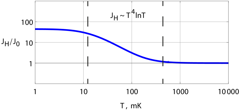
Figure S6: Temperature dependence of electron-phonon heat flow enhanced by the spin-diffusion. Plotted is the ratio of the spin-diffusion part $J_{H}(T)$ and the local part Eq.(51). In the wide temperature region $T_{H}^{(1)}<T<T_{H}^{(2)}$, where $T_{H}^{(1)}\sim 20\,\mathrm{mK}$, $T_{H}^{(2)}\sim 500\,\mathrm{mK}$, the outgoing heat flow $J_{H}(T)\propto T^{4}\,\ln(T/T_{H}^{(1)})$. The parameters of the 2D system were: electron density $n=10^{11}\,\mathrm{cm^{-2}}$, electron effective mass $m=0.1\,m_{0}$, ($m_{0}$ is the free electron mass), the Fermi momentum $1/k_{F}=12\,\mathrm{nm}$, the Fermi energy $E_{F}=2.4\,\mathrm{meV}$, dimensionless conductance $p_{F}l=10$, the Lande $g$-factor $g=5$, the spin-orbit band splitting $\Delta_{R}=0.002\,E_{F}$ (corresponding to the Dresselhaus splitting in InP at the corresponding density); the anisotropy parameters in Eq.(47) are $\gamma_{\parallel}=0$, $\gamma_{\bot}=1$. The magnetic field $H=8\mathrm{T}$ corresponds to $h=0.5$.

For the effects of charge diffusion on the e-ph heat flow in the 2D electron system with no additional screening of interactions($\varepsilon=const$) the situation is similar to that of Eq.(S87):

$$J_{C_{2D}}=\frac{1}{g_{\Box}}\frac{2\pi^{3}p_{F}^{2}}{63\hbar^{6}\rho_{m}v_{s}^{5}}\left(\frac{\varepsilon\hbar v_{F}}{e^{2}}\right)^{2}\left(\frac{\Gamma}{p_{F}v_{F}}\right)^{2}T^{6},$$ (S90)

where the effective dielectric constant is an arithmetic mean of the dielectric constants of the media on both sides of the 2D system: $\varepsilon=(\varepsilon_{1}+\varepsilon_{2})/2$. The enhancement is thus reduced to a temperature-independent factor.

The result is the same for the geometry with additional screening by a metallic gate at temperatures $T\gg\hbar v_{s}/b$ with $b$ being the distance between the 2D electron plane and the gate. At lower temperature $T\ll\hbar v_{s}/b$ the effective dielectric permittivity is $q$-dependent: $\varepsilon(q)=\varepsilon(\coth qb+1)/2\approx\varepsilon/2qb$ which transforms Coulomb interaction into a short-range one, $V_{0}(q)=4\pi e^{2}b$. The behavior becomes similar to Eqs.(S88) however, with the crossover temperature $T_{H}^{(1)}$ replaced by $T_{C}^{(1)}=(1/g_{\Box}k_{F}b)(v_{s}/v_{F})^{2}(\varepsilon\hbar v_{F}/e^{2})E_{F}$:

$$J_{C_{2D+gate}}=\frac{1}{g_{\Box}}\frac{\pi p_{F}^{4}}{240\hbar^{6}\rho_{m}v_{s}^{3}}$$ (S91)

$$\times\frac{1}{k_{F}^{2}b^{2}}\left(\frac{\varepsilon\hbar v_{F}}{e^{2}}\right)^{2}\left(\frac{\Gamma}{p_{F}v_{F}}\right)^{2}T^{4}\ln\frac{T}{T_{C}^{(1)}},\,\qquad T\gg T_{C}^{(1)},$$

$$J_{C_{2D+gate}}=g_{\Box}\frac{2\pi^{3}\Gamma^{2}}{63\hbar^{6}\rho_{m}v_{s}^{7}}T^{6},\,\qquad T\ll T_{C}^{(1)},$$ (S92)

Similarly to (S88), Eq.(S91) contains $\ln T$ coming from the angles $\theta_{C}\sim\sqrt{T_{C}^{(1)}/T}$.

We also note that Eq.(S91),(S92) represent only the Mandelstam-Leontovich contribution due to charge diffusion. At high enough temperatures

$$T>T_{C}^{(2)}\sim T_{C}^{(1)}\,\left(\frac{v_{F}}{v_{s}}\right)$$

this contribution is smaller than the $J^{(0)}_{tr}$ arising from local processes corresponding to the transverse phonon Pippard’s ultrasound attenuation, Eq.(2) in the paper:

$$J_{0}=g_{\Box}\frac{2\pi^{3}p_{F}^{2}}{189\hbar^{6}\rho_{m}v_{s,t}^{5}}T^{6}$$ (S93)

Thus for temperatures $T>T_{C}^{(2)}$ the $T^{6}$ law is restored.

We should note that in real heterostructures the deformation potential $\Gamma$ is in general anisotropic.However, this fact does not lead to any profound changes like suppression of logarithmic behavior $\propto\ln T$ in Eq.(S91). This would require a highly anisotropic deformation potential $\Gamma\propto\sin^{2}\theta$ which we do not expect.

VI VI. A particular example: thin film of $\mathrm{InSb}$.

Here we consider the enhancement of ultrasound attenuation in an $\mathrm{InSb}$ thin film with electron density $n=10^{11}\mathrm{cm^{-2}}$ and thickness $d\geq 10-20\mathrm{nm}$ on the $\mathrm{SiO_{2}}$ substrate. We consider the spin effect of parallel magnetic field applied to the film, so its thickness $d$ is chosen to be relatively small (slightly larger than Fermi wavelength) in order to avoid orbital effects of magnetic field. In spite of the fact that piezoelectric coupling is present in InSb, it is irrelevant for in-plane longitudinal phonons s_piezo as matrix element of piezoelectric interaction for such phonons is equal to zero. Thus, we assume that phonon wavevector ${\bf q}$ is parallel to the 2DEG plane.

Effective mass of $\mathrm{InSb}$ is equal to $\,m=0.014m_{0}$ s_ioffe , spin-orbital band splitting is $\Delta_{SO}\approx 0.11\mathrm{meV}$ s_insb_so1 ; s_insb_so2 and the electron mean-free-path is supposed to be relatively long, $p_{F}l=50$. At such parameters the Fermi energy $\varepsilon_{F}=0.02\,\mathrm{eV}$, while the deformation potential $\Gamma=-13.12\,\mathrm{eV}$ s_dp_insb . A $\mathrm{SiO_{2}}$ substrate is characterized by $v_{s}=6\times 10^{5}\mathrm{cm/s}$ and the effective dielectric constant $\varepsilon=(1+3.9)/2\approx 2.5$. Finally, we use Eqs.(S71) and (S79) with the specified sample/material parameters. The resulting plots are given in the Fig.1 of the main text.

VII VII. A general expression for phonon decay rate: a phenomenological derivation

Here we derive a general expression for ultrasonic attenuation using a phenomenological approach of diffusive electron transport. We start by the system of equations

$$\left\{\begin{aligned} &\partial_{t}n^{(i)}+\mathrm{div}{\bf j}^{(i)}=0,\\ &{\bf j}^{(i)}=-D^{(i)}{\bf\nabla}n^{(i)}+\kappa^{(i)}{\bf F}^{(i)}\\ &U^{(i)}=\int{\cal V}_{0}({\bf r}-{\bf r}^{\prime})\sum\limits_{j}\delta n^{(j)}({\bf r}^{\prime})+\Gamma^{(i)}\,{\rm{div}\bf{u}}\end{aligned}\right.$$ (S94)

Fourier transforming the set we get

$$\left\{\begin{aligned} &(-i\omega+D^{(i)}q^{2})n^{(i)}=-\kappa^{(i)}q^{2}U^{(i)}\\ &U^{(i)}=V_{0}(q)\sum\limits_{j}n^{(j)}({\bf q})+(i{\bf q}\cdot{\bf u})\Gamma^{(i)}\end{aligned}\right.$$ (S95)

Due to Coulomb interaction the solution for i-th branch depends on the dynamics of total density. Thus, the solution is

$$n^{(i)}=-\Pi^{(i)}(\omega,q)\left(\Phi^{(i)}-\Phi_{C}(\omega,q)\right)$$ (S96)

where $\Pi^{(i)}(\omega,q)=\kappa^{(i)}q^{2}/(-i\omega+D^{(i)}q^{2})$ is a response function, $\Phi^{(i)}=(i{\bf q}\cdot{\bf u})\Gamma^{(i)}$,

$$\Phi^{C}=\frac{V_{0}(q)\sum_{i}\Pi^{(i)}\Phi^{(i)}}{1+V_{0}(q)\sum_{i}\Pi^{(i)}}.$$ (S97)

Here $\Phi^{C}$ describes dynamic Coulomb counteraction. To obtain the phonon decay rate we have to evaluate the dissipation power in a unit volume

$$Q_{t}=\frac{1}{2}\sum\limits_{i}{\rm\,Re\,}\left({\bf j}^{(i)}\cdot{\bf F}^{*(i)}\right)=\frac{1}{2}\sum\limits_{i}{\rm\,Re\,}\left[-i\omega(\Phi^{(i)}-\Phi_{C}(\omega,q))\Pi^{(i)}(\Phi^{(i)}-\Phi_{C}(\omega,q))^{*}\right]$$ (S98)

$$=\frac{\omega}{2}\sum\limits_{i}{\rm Im\,}\left[(\Phi^{(i)}-\Phi_{C}(\omega,q))\Pi^{(i)}(\Phi^{(i)}-\Phi_{C}(\omega,q))^{*}\right].$$

and the energy of acoustic wave:

$$E_{w}=\frac{\rho_{m}}{2}\omega^{2}u_{m}^{2}$$ (S99)

Finally, for the phonon decay rate we get

$$\tau_{ph}^{-1}=\frac{Q_{t}}{E_{w}}=\frac{q^{2}}{\rho_{m}\omega}\sum\limits_{i}{\rm Im\,}\left[\Gamma^{(i)}_{s}\Pi^{(i)}(\Gamma^{(i)}_{s})^{*}\right]$$ (S100)

$$=\frac{q^{2}}{\rho_{m}\omega}\sum\limits_{i}\Gamma^{(i)}_{s}{\rm Im\,}\left[\Pi^{(i)}\right](\Gamma^{(i)}_{s})^{*}$$ (S101)

where $\Gamma_{s}=(\Phi^{(i)}-\Phi_{C}(\omega,q))/\,{\rm{div}\bf{u}}$ can be considered as a dynamically screened vertex.

VII.1 A. Multiple branches

We analyze here the case of two quasiparticle branches and very strong bare Coulomb potential, $V(q)\rightarrow\infty$. The Coulomb counteraction term takes the form

$$\Phi^{C}=\frac{\sum_{i}\Pi^{(i)}\Phi^{(i)}}{\sum_{i}\Pi^{(i)}}$$ (S102)

that exactly fixes total density $\delta(n_{1}+n_{2})=0$. Thus the phonon decay rate becomes equal to

$$\tau_{ph}^{-1}=\frac{q^{2}}{\rho_{m}\omega}{\rm Im\,}\left[\frac{(\Gamma_{1}-\Gamma_{2})\Pi_{2}}{\Pi_{1}+\Pi_{2}}\Pi_{1}\frac{(\Gamma_{1}-\Gamma_{2})\Pi_{2}^{*}}{(\Pi_{1}+\Pi_{2})^{*}}\right.+\left.\frac{(\Gamma_{2}-\Gamma_{1})\Pi_{1}}{\Pi_{1}+\Pi_{2}}\Pi_{2}\frac{(\Gamma_{2}-\Gamma_{1})\Pi_{1}^{*}}{(\Pi_{1}+\Pi_{2})^{*}}\right]=\frac{(\Gamma_{1}-\Gamma_{2})^{2}q^{2}}{\rho_{m}\omega}{\rm Im\,}\left[\Pi_{1}^{-1}+\Pi_{2}^{-1}\right]^{-1}$$ (S103)

Using also the fact that $\kappa_{i}=\nu_{i}D_{i}$ we obtain:

$$\tau_{ph}^{-1}=\frac{(\Gamma_{1}-\Gamma_{2})^{2}}{\rho_{m}}\frac{\nu_{*}D_{*}q^{2}}{v_{s}^{2}+(D_{*}q)^{2}}$$ (S104)

where $v_{s}=\omega/q$ is the sound velocity and $\nu_{*}=(\nu_{1}^{-1}+\nu_{2}^{-1})^{-1}$, $D_{*}=\nu_{*}^{-1}((\nu_{1}D_{1})^{-1}+(\nu_{2}D_{2})^{-1})^{-1}$ are the effective density of states and diffusion coefficient respectively. To obtain the total ultrasonic attenuation we also have to take into account the PIC result:

$$(\tau_{ph}^{-1})^{(0)}=c_{l}\frac{p_{F}^{2}}{\rho_{m}}(\nu_{1}D_{1}+\nu_{2}D_{2})q^{2}$$ (S105)

This equation coincides with Eq.(1) of the main text if both electron branches are identical $\nu_{1}=\nu_{2},\,D_{1}=D_{2}$. Thus, for the total attenuation rate we obtain:

$$\tau_{ph}^{-1}=c_{l}\frac{p_{F}^{2}}{\rho_{m}}(\nu_{1}D_{1}+\nu_{2}D_{2})q^{2}+\frac{(\Gamma_{1}-\Gamma_{2})^{2}}{\rho_{m}}\frac{\nu_{*}D_{*}q^{2}}{v_{s}^{2}+(D_{*}q)^{2}}$$ (S106)

and the enhancement factor $\mathcal{F}=\tau_{ph}^{-1}/(\tau_{ph}^{-1})^{(0)}$ is

$$\mathcal{F}_{MB}(q)=1+\frac{1}{c_{l}}\left(\frac{\Gamma_{1}-\Gamma_{2}}{p_{F}v_{F}}\right)^{2}\frac{\nu_{*}D_{*}}{\nu_{1}D_{1}+\nu_{2}D_{2}}\frac{v_{F}^{2}}{v_{s}^{2}+(D_{*}q)^{2}}$$ (S107)

An important particular case is that of the Zeeman splitting by an in-plane magnetic field $H$ for a 2D electron system ($d_{e}=2$). Here an asymmetry appears between the spin-up and spin-down electron branches (while $\nu_{1}=\nu_{2}=\nu$): $\varepsilon_{\uparrow(\downarrow)}=\varepsilon_{F}\pm\mu H/2$, $D_{\uparrow(\downarrow)}=D(1\pm\mu H/2\varepsilon_{F})$. However, the most important asymmetry is the one in the vertex $\Gamma$ that arises from the momentum-dependent part of the electron-phonon coupling:

$$\Gamma_{\uparrow}-\Gamma_{\downarrow}=(\partial\Gamma/\partial\varepsilon_{F})\mu H$$ (S108)

In the simplest model, where the only effect of the strain upon electron spectrum is its overall shift, the density-dependent contribution arises from the stress $\langle p_{\alpha}v_{\beta}\rangle_{FS}$ of electron liquid only:

$$\Gamma(p_{F})=\Gamma_{0}-p_{F}v_{F}/2\rightarrow\partial\Gamma/\partial\varepsilon_{F}=-1$$ (S109)

Introducing the dimensionless magnetic field $h=\mu H/2\varepsilon_{F}$, we arrive at the result

$$\mathcal{F}_{H}(q,h)=1+\frac{v_{F}^{2}h^{2}(1-h^{2})}{v_{s}^{2}+(Dq(1-h^{2}))^{2}}$$ (S110)

Finally we discus the effect of inter-branch scattering. In fact, it modifies the response function

$$\frac{D_{*}q^{2}}{-i\omega+D_{*}q^{2}}\Rightarrow\frac{D_{*}q^{2}}{-i\omega+D_{*}q^{2}+1/2\tau_{so}}$$ (S111)

where $\tau_{SO}$ is the characteristic time of inter-branch mixing so labeled in analogy with the spin-orbit mixing of electron branches with different spin projections. Tt limits the diffusion enhancement factor

$$\frac{D_{*}q^{2}}{\omega^{2}+(D_{*}q^{2})^{2}}\Rightarrow\frac{D_{*}q^{2}}{\omega^{2}+(D_{*}q^{2}+1/2\tau_{so})^{2}}$$ (S112)

and the final result becomes equal to

$$\mathcal{F}_{H}(q,h)=1+\frac{q^{2}v_{F}^{2}h^{2}(1-h^{2})}{(qv_{s})^{2}+(Dq^{2}(1-h^{2})+1/2\tau_{so})^{2}}$$ (S113)

VII.2 B. Imperfect screening

Another case of interest is the case of two quasiparticle branches with identical parameters $\Gamma_{1(2)}=\Gamma,\,\nu_{1(2)}=\nu,\,D_{1(2)}=D$ but finite strength of Coulomb interaction. In this case no asymmetry is present and thus asymmetric electron modes cannot be excited. However, finite Coulomb interaction and incomplete screening allows density fluctuations which diffusive relaxation leads to the enhancement of ultrasound attenuation and the e-ph energy flow:

$$\tau_{ph}^{-1}=\frac{q^{2}}{\rho_{m}\omega}{\rm Im\,}\left[2\times\left(\Gamma-\frac{2V_{0}\Pi\Gamma}{1+2V_{0}\Pi}\right)\Pi\left(\Gamma-\frac{2V_{0}\Pi\Gamma}{1+2V_{0}\Pi}\right)^{*}\right]=\frac{q^{2}}{\rho_{m}\omega}{\rm Im\,}\left[\frac{2\Gamma^{2}\Pi}{|1+2V_{0}\Pi|^{2}}\right]=\frac{\Gamma^{2}}{\rho_{m}}\frac{2\nu Dq^{2}}{v_{s}^{2}+(2\nu V_{0}+1)^{2}(Dq)^{2}}$$ (S114)

$$\mathcal{F}_{C}=1+\frac{d_{e}^{2}}{c_{l}}\frac{(\Gamma/p_{F}v_{F})^{2}}{d_{e}^{2}(v_{s}/v_{F})^{2}+(q^{2}l^{2})(1+2\nu V_{0}(q))^{2}}$$ (S115)

For a 2D geometry and Coulomb interaction $V_{0}(q)=2\pi e^{2}/\varepsilon q$ which is still relatively strong, $\nu V\gg 1$, $\nu V(q)ql\gg s/v_{F}$, the result acquires a simple, frequency-independent form:

$$\mathcal{F}_{C_{2D}}=1+\frac{1}{c_{l}g_{\Box}^{2}}\left(\frac{\varepsilon\hbar v_{F}}{e^{2}}\right)^{2}\left(\frac{\Gamma}{p_{F}v_{F}}\right)^{2}$$ (S116)

where $g_{\Box}$ is dimensionless conductance per square in $e^{2}/h$ units. The expression is valid also for a quasi-2D sample, when the phonon wavelength $\lambda$ is much larger than the width of quasi-2D system $d_{s}$.

In the most general case, the bare Coulomb potential $V_{0}(q)$ acting between conduction electrons can be written in terms of some dispersive dielectric response $\varepsilon(q)$, as $V_{0}(q)=2\pi e^{2}/q\varepsilon(q)$. Therefore Eq.(S116) can be used in order to extract $\varepsilon(q)$ dependence from the measured phonon relaxation rate.

An important special case is presented by a 2D electron gas with a metal gate placed nearby which additionally screens electron-electron interaction. Here $\varepsilon(q)=\varepsilon/(1-e^{-2qb})$ and $V_{0}(q)=(2\pi e^{2}/\varepsilon q)(1-e^{-2qb})$, where $b$ is the distance between electron plane and gate parallel to it. As long as phonon wavelength is shorter than distance $b$, the presence of the gate may be ignored, while for short wavelengths, when $qb\ll 1$, Coulomb interaction becomes effectively-short-range, $V_{0}(q)=4\pi e^{2}b/\varepsilon$. Exactly for this region of low frequencies (temperatures) enhancement factor $\mathcal{F}$ is

$$\mathcal{F}_{C_{2D+gate}}=1+\frac{4(\Gamma/p_{F}v_{F})^{2}}{(v_{s}/v_{F})^{2}+(q^{2}l^{2})(4\pi\nu e^{2}b/\varepsilon)^{2}}$$ (S117)

We see that the crossover between $\mathcal{F}\propto\omega^{-2}$ and $\mathcal{F}\propto\omega^{0}$ behavior emerges at

$$\hbar\omega_{cross}\sim\frac{1}{g_{\Box}}\frac{1}{k_{F}b}\left(\frac{v_{s}}{v_{F}}\right)^{2}\left(\frac{\varepsilon\hbar v_{F}}{e^{2}}\right)E_{F}.$$

This equation can be used for an experimental determination of the background dielectric constant $\varepsilon$.

References

(1) A. Schmid, Z. Physik 259, 421 (1973).
(2) M. Reyzer and A. V. Sergeev, Zh. Exp. Theor. Fiz. 92, 2291 (1987)
[Sov. Phys. - JETP 65, 1291 (1987)]
(3) V. I. Yudson and V. E. Kravtsov, Phys. Rev. B 67, 155310 (2003)
(4) A. B. Pippard,
Philos. Mag., 46 (1955) 1104.
(5) A. I. Akhiezer, M. I. Kaganov and G. Ya. Lyubarskyi,
ZhETF, 32, 837 (1957).
(6) M. E. Gershenson, D. Gong, T. Sato, B. S Karasik, A. V. Sergeev,
App. Phys. Lett., 79, 2049 (2001)
(7) A. Savin, J. Pekola, M. Prunnila, J. Ahopelto and P. Kivinen,
Physica Scripta, T114, 57 (2004).
(8) M. Ovadia, B. Sacepe and D. Shahar,
Phys. Rev. Lett. 102, 176802 (2009)
(9) D. V. Khveshchenko and M. Reizer,
Phys. Rev. B 56, 15822 (1997)
(10) M. E. Gershenson, Yu. B. Khavin, D. Reuter, P. Schafmeister, and A. D. Wieck,
Phys. Rev. Lett. 85, 1718 (2000)
(11) L. D. Landau and E. M. Lifshitz, Fluid Mechanics, (Pergamon, Oxford, 1977).
(12) A. Sergeev, M. Yu. Reizer and V. Mitin,
Phys. Rev. Lett. 94, 136602 (2005).
(13) M. Prunnila, P. Kivinen, A. Savin, P. Torma, and
J. Ahopelto,
Phys. Rev. Lett. 95, 206602 (2005);
M. Prunnila,
Phys. Rev. B 75, 165322 (2007).
(14) A. Sergeev, V. Mitin,
Europhys. Lett., 51, 641 (2000).
(15) For application of kinetic approach see e.g. A. D. Semenov, G. N. Goltsman and R. Sobolewski,
Supercond. Sci. Technol., 15, R1 (2002).
(16) In the case of 2D electron gas we consider an array of 2D electron planes with the distance between them. Then in Eq.(1) .
(17) E. I. Blount, Phys. Rev. 114, 418 (1959).
(18) T. Tsuneto, Phys. Rev.121, 402 (1960).
(19) M. Cardona and N. E. Christensen,
Phys. Rev. B 35, 6182 (1987).
(20) See online supplementary material to this paper.
(21) A. Sergeev and V. Mitin,
Phys. Rev. B 61, 6041 (2000).

References

(1) A. Schmid, Z. Physik 259, 421 (1973).
(2) M. Reyzer and A. V. Sergeev, Zh. Exp. Theor. Fiz. 92, 2291 (1987)
[Sov. Phys. - JETP 65, 1291 (1987)]
(3) V. I. Yudson and V. E. Kravtsov, Phys. Rev. B 67, 155310 (2003)
(4) T. Tsuneto, Phys. Rev.121, 402 (1960).
(5) Alex Kamenev, Alex Levchenko, Advances in Physics (2009)
Volume: 58, Issue: 3 (Taylor & Francis).
(arxiv.org/abs/0901.3586)
(6) We assume that phonon distribution function is an equilibrium one, either due to phonon-phonon inelastic scattering, or
due to the role of external phonon bath.
(7)
Piezoelectric coupling may be incorporated in our scheme, in this case vertex will depend on phonon momentum and one will have to replace
constant by the -dependent function.
(8) M. A. Skvortsov, JETP Lett., 67 (2), 133-139 (1998).
(9) D. V. Khveshchenko and M. Reizer,
Phys. Rev. B 56, 15822 (1997)