Parameter identification in large kinetic networks with BioPARKIN

Abstract

Motivation.

Modelling, parameter identification, and simulation play an important role in systems biology. Usually, the goal is to determine parameter values that minimise the difference between experimental measurement values and model predictions in a least-squares sense. Large-scale biological networks, however, often suffer from missing data for parameter identification. Thus, the least-squares problems are rank-deficient and solutions are not unique. Many common optimisation methods ignore this detail because they do not take into account the structure of the underlying inverse problem. These algorithms simply return a “solution” without additional information on identifiability or uniqueness. This can yield misleading results, especially if parameters are co-regulated and data are noisy.

Results.

The Gauss-Newton method presented in this paper monitors the numerical rank of the Jacobian and converges locally, for the class of adequate problems, to a solution that is unique within the subspace of identifiable parameters. This method has been implemented in BioPARKIN, a software package that combines state-of-the-art numerical algorithms with compliance to system biology standards, most importantly SBML, and an accessible interface.

Availability.

The software package BioPARKIN is available for download at
 http://bioparkin.zib.de .

1 Introduction

Following [1], there are two main modelling approaches in systems biology. On one hand, there exist detailed models for isolated parts of a system. The states and model parameters of such systems are generally well-defined, but the system is far from being closed and there are great variations in the environmental conditions. On the other hand, large-scale networks are more closed, but suffer from missing data for parameter identification. Biological data, however, often indicate that parameters are correlated, and that a system’s behaviour can be characterised by a few control parameters. In contrast to parameter optimisation, parameter identification not only aims at the determination of parameter values from given measurement data, but also on the detection of dependencies between parameters. As stated in [1], the identification of all control parameters which allow a proper characterisation of the states of a biological system, is by no means trivial and, at least for most applications, an open problem.

Modelling, parameter estimation and simulation of biological systems have become part of modern systems biology toolboxes. Unfortunately, many of these programs are based on inefficient or mathematically outdated algorithms. To counteract this problem, we have developed the software package BioPARKIN¹ [2]. This software is a renewed version of the former codes LARKIN [3] and PARKIN [4], which have successfully been applied in chemical industry for more than 20 years [5].

BioPARKIN combines a basis of long-standing mathematical principles with compliance to system biology standards, most importantly SBML [6], and an accessible interface. The SBML format is one of the most important standards in systems biology to facilitate collaboration of researchers at all levels (physicians, biologists, mathematicians, etc.). The interface strives to wrap complicated structures and settings (especially with regard to the numerical back-end) into an user-friendly package that can be used correctly by non-mathematicians.

BioPARKIN is split into two parts – the numerical library PARKINcpp and the graphical user interface (GUI) – in order to achieve several advantages. The crucial, yet computation-intensivenumerical algorithms are embedded in an efficient C++ library while the GUI is coded in Python which enables rapid interface changes when adapting the user interface to new insights into user behaviour. Another important advantage is the independent availability of the PARKINcpp library for use in other related projects. Both parts are available under the LPGL which is a flexible open-source license allowing for the use of the software in both open and closed (i.e. commercial) projects.

The core of PARKINcpp and its unique feature is the solver NLSCON for nonlinear least-squares with constraints [7]. This Gauss-Newton type method is especially suited for rank-deficient problems [8]. NLSCON requires, however, some user specified input such as threshold values for species and parameters, or a threshold value for rank decision. In order to choose reasonable values and to obtain reliable results, it is indispensable to understand the foundations of the algorithm. This paper therefore aims at giving an overview of the functionality and implementation of NLSCON within BioPARKIN.

The article is organised as follows. We start with the problem definition in Section 2. In Section 3 we explain our method to solve nonlinear least-squares problems. Finally, we present and discuss numerical results in Section 4.

2 Approach

2.1 Large kinetic networks

A major topic in systems biology is the study of the dynamical evolution of bio-chemical mechanisms within a well-defined, biology-related context. The bio-chemical mechanisms in such a compound under consideration are typically given as a, possibly huge, set of chemical reactions between numerous species forming a large kinetic network. Assuming the general principle of mass action kinetics, this large network transforms readily to a system of $n$ ordinary differential equations (ODEs) leading to an autonomous initial value problem (IVP)

$$y^{\prime}=f(y\,;\,p),\qquad y(t_{0})=y_{0},\qquad p\in\mathbb{R}^{q}$$ (2.1)

where the rate of change in the species vector, $y^{\prime}\in\mathbb{R}^{n}$, is described by the term on the right-hand side, $f(y;p)$, depending on both the species, $y\in\mathbb{R}^{n}$, and the parameter vector, $p\in\mathbb{R}^{q}$. The initial condition vector, $y_{0}$, has the same dimension as the species vector $y$. In BioPARKIN, the ODE systems are solved numerically with LIMEX, a linearly implicit Euler method with extrapolation that is especially suited for stiff differential equations [9, 10, 11]. LIMEX is a numerical integrator with adaptive stepsize control that allows for a computation of the solution $y$ at arbitrary time points with prescribed accuracy by using an appropriate interpolation scheme. This is often not possible with other ODE solvers. LIMEX can be applied to differential-algebraic equations as well, which allows for the processing of algebraic constraints in BioPARKIN.

It is assumed that some discrete experimental data (in form of species concentrations versus time),

$$(\tau_{1},z_{1}),\,\ldots,\,(\tau_{M},z_{M}),$$ (2.2)

are available. Note that frequently only a certain amount of the $n$ species concentrations are measurable observables, if at all. The task at hand now reduces to quantify the $q$ unknown components of the parameter vector, $p$, by comparison between computed model values and measured data.

A complete data set, of course, must include prescribed statistical tolerances, $\delta z_{j}\,(j=1,\ldots,M)$, for each measurement as well. The mathematically correct handling of these will be described in Section 2.2.

Breakpoint handling.

A sudden event (maybe from outside the biological system) is handled by introducing a breakpoint, $t_{b}>t_{0},$ and subsequently, splitting the ODE system into a $y^{-}$-part for $t_{0}<t\leq t_{b}$, and a $y^{+}$-part for $t_{b}<t$,

$$(y^{-})^{\prime} = f(y^{-};\,p),\qquad y^{-}(t_{0})=y_{0}$$ (2.3)

$$(y^{+})^{\prime} = f(y^{+};\,p),\qquad y^{+}(t_{b})=g(y^{-}(t_{b})\,;\,p)$$ (2.4)

where $g:\mathbb{R}^{n}\times\mathbb{R}^{q}\longrightarrow\mathbb{R}^{n}$ is a mapping of the initial conditions, possibly dependent on the parameter vector, $p$. Note that, in BioPARKIN, breakpoints have to be defined beforehand and hence, they must be independent of the time course of $y$. This approach of splitting the ODE system with respect to time particularly applies in case of multiple experiments.

In SBML such breakpoints are defined via “events” with trigger expressions in the form

$\mathtt{eq(time,t_{b})}.$

Many other present simulation tools cannot handle this kind of event because the numerical integrator simply does not stop at time $t_{b}$.

Multiple experiments.

The design of experiments almost always includes different conditions such that the effects of these different conditions on the system under investigation can be observed and studied. In the simplest case, calibration measurements might be necessary, for example, or data related to different initial conditions, $y_{0,1},y_{0,2},\ldots,y_{0,\nu},\ldots$, are given. Numerically, these situations can be handled by the concatenation of several IVPs,

$$y_{\nu}^{\prime}=f_{\nu}(y_{\nu}\,;\,p),\qquad y_{\nu}(t_{0,\nu})=y_{0,\nu},\quad\nu=1,2,\ldots,$$ (2.5)

very similar to the management of breakpoints/events. If required, the solution $y_{\nu}$ corresponding to the (virtual) initial timepoint, $t_{0,\nu}$, can readily be shifted to the (original) initial time, $t_{0}$, for comparison or plotting purposes.

2.2 Parameter identification

Following the fundamental idea of Gauss, parameter identification is, as implemented in BioPARKIN, equivalent to solving the weighted least-squares problem,

$$\frac{1}{M}\sum_{j=1}^{M}\|D_{j}^{-1}\big{(}y(\tau_{j}\,;\,p)-z_{j}\big{)}\|_{2}^{2}=\min,$$ (2.6)

with diagonal weighting $(n,n)$-matrices,

$$D_{j}:=\mathrm{diag}\big{(}(\delta z_{j})_{1},\,\ldots,\,(\delta z_{j})_{n}\big{)},\qquad j=1,\ldots,M.$$ (2.7)

Note that, if not all components of a datum, $z_{j}\in\mathbb{R}^{n}$, are available at a specific measurement time point, $\tau_{j}$, then the missing data in the least-squares formulation is simply replaced by the computable model value, therefore effectively neglecting the corresponding contribution in the sum of Equation (2.6). The corresponding entry in $D_{j}$ is then set to one.

If, on the other hand, a component of given error tolerance, $\delta z_{j}$, or even the whole vector, is put to zero, this contribution to the sum in Equation (2.6) is also taken out, and considered as a (nonlinear) equality constraint to the least-squares formulation instead.

In the (hopefully rare) case of missing error tolerances in the data file, the measurement tolerances are simply set to

$$\big{(}\delta z_{j}\big{)}_{\ell}=\max\big{\{}\big{|}\big{(}z_{j}\big{)}_{\ell}\big{|},\,\mathrm{thres}(y_{\ell})\big{\}},\quad\ell=1,\ldots,n,$$ (2.8)

with some user specified threshold mapping, $\mathrm{thres}(y_{\ell})$. If this threshold value is not defined, it is set to zero.

The least-squares problem (2.6) may be written even more compactly as

$$\|F(p)\|_{2}^{2}\equiv F(p)^{{}^{T}}F(p)=\min,$$ (2.9)

where $F\,:\,\mathbb{R}^{q}\rightarrow\mathbb{R^{L}}$ is a nonlinear mapping and structured as a stacked vector of length $L=nM$,

$$F(p)=\left[\begin{array}[]{c}D_{1}^{-1}\big{(}y(\tau_{1}\,;\,p)-z_{1}\big{)}\\ \vdots\\ D_{M}^{-1}\big{(}y(\tau_{M}\,;\,p)-z_{M}\big{)}\end{array}\right].$$ (2.10)

If not all components of a measurement, $z_{j}$, are given, the number $L$ will accordingly be smaller, $L<nM$.

2.3 Parameter constraints

In order to enforce constraints such as positivity or upper and lower bounds on the unknown parameters to be determined in the model, a (differentiable) transformation, $\varphi:\mathbb{R}^{q}\longrightarrow\mathbb{R}^{q}$, can be introduced resulting in a different parametrisation, $u$, of the model ODE system,

$$p=\varphi(u),\quad y^{\prime}=f(y\,;\,\varphi(u))=\tilde{f}(y\,;\,u)$$ (2.11)

A global positivity constraint on the parameter vector, $p$, can be achieved, for example, by the (component-wise) exponential transformation

$$p_{i}=\exp(u_{i}),\qquad i=1,\ldots,q$$ (2.12)

To impose an upper and a lower bound, $A$ and $B$, respectively, a sinusoidal transformation

$$p_{i}=A+\frac{B-A}{2}\,\left(1+\sin u_{i}\right),\qquad i=1,\ldots,q$$ (2.13)

can be used. For a single bound, $C$, as last example in this section, a root square transformation

$$p_{i}=C\pm\left(1-\sqrt{1+u_{i}^{2}}\right),\qquad i=1,\ldots,q$$ (2.14)

(with the upper sign for an upper bound and the lower sign for a lower bound) is possible.

The last two transformation formulas are especially eligible since, at least for small perturbations $\mathrm{d}p_{i}\approx\varphi^{\prime}\,\mathrm{d}u_{i}$, the differentials are bounded and, most importantly, are essentially independent of the new parametrisation, $u$.

Note that the application of any transformation of the parameters obviously changes the sensitivities of the parameters to the dynamical evolution of the ODE system. Therefore, it is strongly recommended that parameter constraints should only be applied in order to prevent the parameter vector components, $p_{i}$, from taking on physically meaningless values. The better choice in this case would be to change the model equations since model and data seem to be incompatible.

2.4 Parameter scaling

In general, a scaling-invariant algorithm, i.e. an algorithm that is invariant under the choice of units in a given problem, is (almost) indispensable to guarantee any reliable results. Therefore, the following scaling strategy within the course of the Gauss-Newton iteration has been implemented: in each iteration step $k$, an internal weighting vector, $pw\in\mathbb{R}^{q}$, is used to define local scaling matrices, $W_{k}$ , by

$$W_{k}=\mathrm{diag}(pw_{1},\ldots,pw_{q})$$ (2.15)

with locally given

$$pw_{i}:=\max\left\{|p_{i}^{k}|,\>\mathrm{thresh}(p_{i})\right\},\qquad i=1,\ldots,q$$ (2.16)

where $p_{i}^{k}$ are the current parameter iterates, and ${\mathrm{thresh}(p_{i})>0}$ are suitable threshold values for scaling chosen by the user. Consequently, any relative precision of parameter values below these prescribed threshold values will be meaningless.

3 Methods

3.1 Affine covariant Gauss-Newton algorithm

Starting with an initial guess, $p^{0}\in\mathbb{R}^{q}$, the (damped) Gauss-Newton method is given as

$$p^{k+1}=p^{k}+\lambda_{k}\Delta p^{k},\qquad k=0,1,\ldots$$ (3.1)

Here, the step-length, $0<\lambda_{k}\leq 1$, is recomputed successively in each iteration (see below). The update, $\Delta p^{k}$, is the minimum norm solution to the linear least-squares problem,

$$\|F^{\prime}(p^{k})\,\Delta p^{k}+F(p^{k})\|\binrel@{=}\binrel@@{\mathop{\kern 0.0pt=}\limits^{!}}\min.$$ (3.2)

The $(L\times q)$-Jacobian matrix, $F^{\prime}(\cdot)$, can be approximated by stacking the rows of the sensitivity matrices, $S(\tau_{j})$, corresponding to the measurement points $(\tau_{j},\,z_{j})$,

$$J=\left[\begin{array}[]{c}D_{1}^{-1}S(\tau_{1})\\ \vdots\\ D_{M}^{-1}S(\tau_{M})\end{array}\right].$$ (3.3)

Herein the sensitivity matrices, $S(\tau_{j})$, are samples of the solution trajectories of the inhomogeneous variational equation

$$S^{\prime}=f_{y}\Big{(}y(t\,;\,p^{k})\,;\,p^{k}\Big{)}S+f_{p}\Big{(}y(t\,;\,p^{k})\,;\,p^{k}\Big{)},\quad S(t_{0})=0$$ (3.4)

taken at the measurement time points, $\tau_{j}$. The terms $f_{y}$ and $f_{p}$ on the right hand side are computed analytically by symbolic differentiation. The variational equation is solved simultaneously with the IVP (2.1), representing an ODE system of $((n+1)\times q)$ equations in total. To avoid expensive factorisations of the iteration matrix within LIMEX, it is replaced by its block-diagonal part, as proposed in [12]. The linearly-implicit extrapolation algorithm allows such an approximation, as long as the characteristics of the dynamic system are preserved, which is satisfied here. By using this sparsing, the effort required for sensitivity evaluation does not grow quadratically with the number of parameters, $q$, but only linearly. Hence, reasonable computing times are achieved (compare also Table 2).

For reasons of comparison with other software tools, the Jacobian matrix can alternatively be approximated by computing the difference quotient, for $\ell=1,\ldots,L$ and $i=1,\ldots,q$,

$$J_{\ell,i}=\frac{1}{h}\Big{(}F_{\ell}(p+e_{i}h)-F_{\ell}(p)\Big{)},\qquad h=\mathcal{O}\Big{(}\left|p_{i}\right|\cdot\sqrt{\mathrm{eps}}\Big{)},$$ (3.5)

whereby $\mathrm{eps}$ it the relative machine precision. In BioPARKIN, the user can optionally invoke a feedback strategy in which the finite difference disturbance is additionally adapted to the current values of $F_{\ell}$.

All approaches to compute the Jacobian matrix make sure that, at each current parameter estimation, $p^{k}$, the approximation $J\approx F^{\prime}(p^{k})$ is valid. Note, however, that the Jacobian computed by numerical differentiation is generally less accurate than the Jacobian obtained via the variational equation.

In passing, the notation of the so-called simplified Gauss-Newton correction, $\overline{\Delta p}^{k+1}$, as the minimum norm solution to

$$\|J(p^{k})\,\overline{\Delta p}^{k+1}+F(p^{k+1})\|\binrel@{=}\binrel@@{\mathop{\kern 0.0pt=}\limits^{!}}\min,$$ (3.6)

may also be introduced for later use.

3.2 Threshold-related scaling

Often, model species and model parameters cover a broad range of physical units and their values can vary over orders of magnitude. To achieve comparability, the sensitivity values have to be normalised by the absolute values of species and parameters to obtain scaled sensitivity matrices,

$$S_{ij}(t)=\left(\frac{\partial y_{i}}{\partial p_{j}}\right)(t)\cdot\frac{\max\{|p_{j}|\,,\,\mathrm{thres}(p_{j})\}}{\max\{\max\limits_{t\in I}|y_{i}(t)|\,,\,\mathrm{thres}(y_{i})\}}$$ (3.7)

where $\mathrm{thres}(\cdot)$ are user-specified threshold values for parameters and species, respectively, and the integration time interval of the ODE system, $I$, is used. In BioPARKIN, the absolute values of these scaled sensitivity values are displayed (see Figure 4 as an example).

3.3 Subcondition monitor

For the solution of the linear least-squares problem in each iteration step, a QR-decomposition of the associated Jacobian $(L,q)$-matrix, $J=F^{\prime}(p)$,

$$Q\,J\,\Pi=\left(\begin{array}[]{c}R\\ 0\end{array}\right)$$ (3.8)

by applying Householder reflections with additional column pivoting is realised in BioPARKIN. Here, for simplicity, the full rank case is assumed where $q\leq L$ and $R$ is an upper triangular $(q,q)$-matrix, $R=(r_{ij})$. The permutation, $\Pi$, is determined such that

$$|r_{11}|\geq|r_{22}|\geq\ldots\geq|r_{qq}|.$$ (3.9)

For some required accuracy, $\delta>0$, given by the user, the numerical rank, $\ell:=\mathrm{rnk}(J)$, indispensable to the successful solution of ill-posed problems, is then defined by the inequality

$$|r_{\ell+1,\ell+1}|<\delta\,|r_{11}|\leq|r_{\ell\ell}|.$$ (3.10)

In general, the maximum of all given measurement tolerances, $\delta z_{j}$, is a suitable choice for this accuracy, $\delta:=\max\limits_{i,j}\{(\delta z_{j})_{i}\}$. In BioPARKIN, however, this choice is left to the user, who has to specify a tolerance XTOL. This tolerance is assigned to $\delta$.

Note that this definition of the numerical rank is highly biased by both row and column scaling of the Jacobian. Introducing, nevertheless, the so-called subcondition number, for $\ell=q$, by

$$\mathrm{sc}(J):=\frac{|r_{11}|}{|r_{qq}|}\leq\mathrm{cond}_{2}(J),$$ (3.11)

it follows that, if $\delta\cdot\mathrm{sc}(J)\geq 1$, the Jacobian will certainly be rank-deficient. In this case, a rank-deficient pseudo-inverse is realised in BioPARKIN, either by a QR-Cholesky variant or by a QR-Moore-Penrose variant [13]. Both cases of pseudo-inverses of the Jacobian, $J$, will be denoted by $\left(J^{\ell}\right)^{+}$.

3.4 Steplength strategy

In order to determine an optimal damping parameter, $0<\lambda_{k}\leq 1$, in each Gauss-Newton step, a first estimate $\lambda_{k}^{(0)}$ is calculated in BioPARKIN from a theoretical prediction on the basis of the former iterate step,

$$\begin{array}[]{rcl}\lambda_{k}^{(0)}&=&\min\{1,\mu_{k}\}\\[8.61108pt] \mu_{k}&:=&\left[\|\Delta p^{k-1}\|\,\|\overline{\Delta p}^{k}\|\,/\,(\,\rho_{k}\,\|\Delta p^{k}\|\,)\right]\cdot\lambda_{k-1}\\[8.61108pt] \rho_{k}&:=&\left\|\left[I_{q}-J(p^{k})^{+}J(p^{k-1})\right]\overline{\Delta p}^{k}\right\|\,.\end{array}$$ (3.12)

If this first a priori estimate, $\lambda_{k}^{(0)}$, fails in the natural monotonicity test,

$$\left\|\overline{\Delta p}^{k+1}\right\|<\left\|\Delta p^{k}\right\|\,,$$ (3.13)

then an additional correction strategy is invoked to compute the a posteriori estimates,

$$\lambda_{k}^{(\nu)}=\min\left\{1\,,\,\frac{1}{2}\lambda_{k}^{(\nu-1)},\ ,\frac{1}{2}\mu_{k}^{(\nu-1)}\right\},\qquad\nu=1,2,\ldots$$ (3.14)

where

$$\mu_{k}^{(\nu-1)}:=\frac{\|\Delta p^{k}\|}{\|\overline{\Delta p}^{k+1,\nu-1}-(1-\lambda_{k}^{(\nu-1)})\,\Delta p^{k}\|}\cdot(\lambda_{k}^{(\nu-1)})^{2}\,.$$ (3.15)

For details see [8] and [2].

As experience shows, the a posteriori loop is rarely activated. To avoid an infinite loop, however, it is ensured that both estimates, $\lambda_{k}^{(0)}$ and $\lambda_{k}^{(\nu)}$, $\nu=1,2,\ldots$, always satisfy the condition

$$\lambda_{k}^{(\nu)}\geq\lambda_{\mathrm{min}},\qquad\nu=0,1,2,\ldots$$ (3.16)

with a minimal permitted damping factor, $\lambda_{\mathrm{min}}$, provided by the user. In case $\lambda_{k}^{(\nu)}<\lambda_{\mathrm{min}}$ deliberate rank reduction is invoked, which usually leads to larger damping factors. Otherwise, the Gauss-Newton iteration will be stopped.

3.5 Deliberate rank reduction

A deliberate rank reduction may additionally help to avoid an iteration towards an attractive point, $\hat{p}$, where the associated Jacobian matrix, $J(\hat{p})$, becomes singular. The general idea of this device is to reduce the maximum permitted rank in the $QR$ decomposition until the natural monotonicity will be fulfilled again or, of course, no further rank reduction is possible. The subroutine as implemented in BioPARKIN is as follows.

To start with, let $q$ denote the current rank. The ordinary Newton correction, $\Delta p^{k}$, is then recomputed with a prescribed maximum allowed rank, $\ell=q-1$. With the new (trial) correction, $\Delta p^{k,\ell}$, a new a priori damping factor, a new trail iterate, and a new simplified correction,

$$\lambda_{k}^{(0,\ell)} = \min\left\{1,\,\mu_{k}^{(0,\ell)}\right\},$$ (3.17)

$$p^{(0,\ell)} = p^{k}+\lambda_{k}^{(0,\ell)}\Delta p^{k,\ell},$$ (3.18)

$$\Delta p^{k,\ell} = -J^{\ell}(p^{k})^{+}F(p^{k}),$$ (3.19)

$$\overline{\Delta p}{}^{(0,\ell)} = -J^{\ell}(p^{k})^{+}F(p^{(0,\ell)}),$$ (3.20)

are computed, respectively.

If now the monotonicity test is successfully passed, the Gauss-Newton iteration proceeds as usual. Otherwise, the damping factors, $\lambda_{k}^{(\nu,\ell)}(\nu=1,2,\ldots)$, are calculated using the a posteriori estimates as given above. If in the a posteriori loop, in turn, $\lambda_{k}^{(\nu,\ell)}<\lambda_{\mathrm{min}}$ occurs, the maximum allowed rank is further lowered by one and, again, the repetition of the rank reduction step starts once more.

This rank reduction procedure is carried out until natural monotonicity, $\|\overline{\Delta p}^{(\nu,\ell)}\|\leq\|\Delta p^{k,\ell}\|$, holds true or, alternatively, a final termination criterion, $\ell<\ell_{\mathrm{min}}\,(0<\ell_{\mathrm{min}}<q)$, is reached.

Note that an emergency rank reduction can occur in a step where the rank of the Jacobian, $J(p^{k})$, has already been reduced because of the subcondition criterion.

3.6 Convergence

Table 1: Typical protocol of parameter identification run with full data, here for the model EpoRcptr (cf. Section 4.4).

• G-N It.	Normf		Normx	Damp. Fctr.	Rank
  0	4.1941414e+01		2.115e-02		6
  1	4.1936708e+01	*	2.094e-02	0.01000
  1	4.1936708e+01		2.469e-02		6
  2	4.1751843e+01	*	1.669e-02	0.41932
  2	4.1751843e+01		3.373e-02		6
  3	4.1655239e+01	*	2.266e-02	0.42693
  3	4.1655239e+01		1.024e-01		6
  4	4.1639220e+01	*	7.410e-02	0.19117
  4	4.1639220e+01		1.076e-01		6
  5	4.1631470e+01	*	4.854e-02	0.37178
  5	4.1631470e+01		1.538e-02		6
  6	4.1547355e+01	*	1.816e-03	1.00000
  6	incompatibility factor: 0.14248
  6	4.1547355e+01		6.366e-03		6
  7	4.1542667e+01	*	2.140e-04	1.00000
  7	incompatibility factor: 0.42707
  7	4.1542667e+01		3.339e-05		6
  8	4.1542118e+01	.	1.783e-08	1.00000
  8	incompatibility factor: 0.00526

• Requested identification accuracy has been $\mathrm{xtol}=10^{-4}$. A star in the third column indicates values corresponding to simplified Gauss-Newton corrections.

As the solution $p^{\ast}$ is approached, the Gauss-Newton method converges linearly with an asymptotic convergence factor $\kappa(p^{\ast})$. This quantity $\kappa$, called incompatibility factor, is monitored by NLSCON and must be smaller than 1 to obtain convergence. Problems that satisfy this condition are called adequate problems. If model and measurement values match exactly, i.e. $F(p^{\ast})=0$, then $\kappa(p^{\ast})=0$ and the method converges quadratically just as Newton’s method. This so-called compatible case, however, does not occur in practice since experimental measurements are never exact. For inadequate nonlinear least-squares problems, the adaptive damping strategy will typically yield values $\lambda_{k}\approx 1/\kappa<1$, and too small damping factors result in fail of convergence. Vice versa, this effect can be conveniently taken as indication of the inadequacy of the inverse problem under consideration [8]. In this case, model equations or the initial parameter guess $p^{0}$ should be changed. A typical NLSCON output protocol in case of successful convergence is shown in Table 1. In the convergent phase, the damping factors approach 1 and finally $\kappa<1$.

4 Results of numerical experiments

Table 2: Comparison of computing times w.r.t. different models.

• 	GynCycle	BovCycle	BIOMD008	EpoRcptr
  Model Characteristics
  #Species	33	15	5	7
  #Parameters	114	60	21	9
  #Reactions	54	28	13	9
  Simulation
  BioPARKIN0 (adpt. $h$)	3.2s	0.8s	0.1s	0.1s
  COPASI1 ($h=10^{-2}$)	1.4s	0.6s	0.2s	0.2s
  COPASI2 ($h=10^{-3}$)	7.2s	4.0s	1.4s	1.1s
  Sensitivity
  BioPARKIN
  $(*)$ (var. eq., overview)	49s	12.9s	0.7s	1.7s
  (var. eq., overview)	117s	29.2s	0.9s	2.0s
  (num. diff., overview)	309s	35.4s	0.8s	0.2s
  COPASI1 (grand total)	94s	18.1s	1.0s	0.3s
  COPASI2 (grand total)	328s	115.6s	8.3s	1.5s

• Benchmark times are rounded to one decimal. Integration was done in [0,100] with time units [s] or [d], accordingly. For comparison reasons, $\mathtt{rtol}=10^{-6}$ and $\mathtt{atol}=10^{-12}$ have been used in all rows (except $(*)$) as accuracy for the ODE solvers. COPASI run times have been measured by batch processing, excluding the time spent for file I/O.

• In COPASI, sensitivities were computed by numerical differentiation. In BioPARKIN, sensitivities were computed by either solving the variational equation (var. eq.) or by numerical differentiation (num. diff.). In a sensitivity overview, sensitivities are plotted over the complete time interval (for an example, see Figure 4).

• $(*)$ Var. Eq. computing times: values have been achieve with slightly lower but still more than sufficient accuracy ($\mathtt{rtol}=10^{-5}$, $\mathtt{atol}=10^{-7}$).

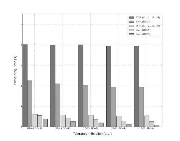
Figure 1: BovCycle: Computing times for the BovCycle model w.r.t. different integrator tolerances. The cases BioPARKIN₁ and BioPARKIN₂ are interpolating at exactly as many sample points as requested for the COPASI_j $(j=1,2)$ cases, respectively, in addition to the adaptive time points. Note that these artificially high numbers of sample points are unusual and absolutely unnecessary for trajectory computations with BioPARKIN and that, for comparision reasons only, these numbers have been applied here. Additionaly, BioPARKIN₀ denotes the timings in case of no interpolation at all.

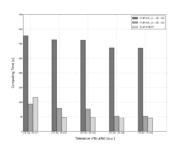
Figure 2: GynCycle: Computing times for the variational equation w.r.t. different integrator tolerances. Note that BioPARKIN integrates the variational equation system while COPASI takes finite differences for the computation.

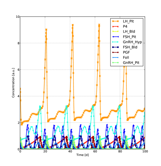
Figure 3: BovCycle: Trajectories of model simulation of selected species.

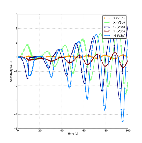
Figure 4: BIOMD008: Sensitivity trajectories of the variational equation w.r.t. parameter V3p.

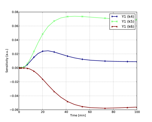
Figure 5: EpoRcptr: Sensitivity trajectories of measurement variable $Y_{1}$.

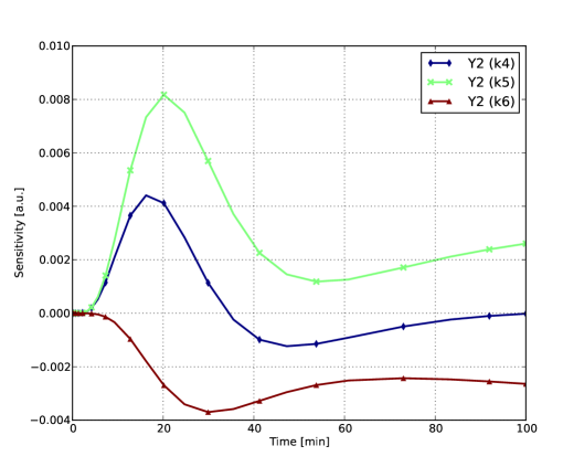
Figure 6: EpoRcptr: Sensitivity trajectories of measurement variable $Y_{2}$.

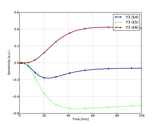
Figure 7: EpoRcptr: Sensitivity trajectories of measurement variable $Y_{3}$.

This section illustrates the use of BioPARKIN and PARKINcpp with actual models. First, two models developed by the Computational Systems Biology group at Zuse Institute Berlin are presented. Next, a third model was obtained from the BioModels database, a website with curated SBML models [14]. And last but not least, a variant of a EPO receptor model from the same database is taken, as it was already published in [15]. All subsequent computations have been performed on an Intel Core 2 Dual CPU (T7200 @ 2.0GHz). In addition, for comparison reason, all forward simulations have been repeated by using COPASI [16]. Note that the stiff ODE solver LSODAR [17, 18] is used in COPASI in contrast to LIMEX. In fact, it seems that, for the computation of any model trajectories, the researcher is forced to supply an equidistant time grid in COPASI. Thereby, the accuracy of the ODE solution, as set by the user in the values $\mathtt{atol}$ and $\mathtt{rtol}$, can easily be foiled in the sense that essential details of model trajectories are simply neglegted in COPASI if the chosen equidistant time grid happens to be too coarse. Note that this is surely not contradicting that the computed ODE solution, at the given sample points, of course, is in fact within the requested accuracy and that, even more surprisingly, the ODE solver LSODAR internally proceeds adaptively. In contrast, simply avoiding all these problems, LIMEX integrates fully adaptive, and Hermite interpolation of appropriate order is applied where necessary, strictly respecting the requested accuracy. Moreover, the fully adaptive approach (i.e. its implementation in BioPARKIN, at least) seems to be much more efficient, see Table 2 and Figures 1, 2.

4.1 GynCycle

Description of the model.

GynCycle is a differential equation model that describes the feedback mechanisms between a number of reproductive hormones and the development of follicles and corpus luteum during the female menstrual cycle [19]. The model correctly predicts hormonal changes following administration of single and multiple doses of two different drugs.

BioPARKIN and the model.

The model GynCycle is fairly large. It contains 33 species, 2 assignment rules, 114 parameters, and 54 reactions. The related benchmark timings for a forward simulation run and sensitivity calculations can be found in Table 2.

Here, BioPARKIN served as a tool to explore the model and its parameter space. Together with its predecessor POEM (an unreleased, in-house tool based on the same numerical principles), it was able to develop and to fine-tune a highly descriptive and predictive model for a complex human pathway that has direct relevance to real-world applications.

4.2 BovCycle

Description of the model.

The model BovCyle is a mechanistic mathematical model of the bovine estrous cycle that includes the processes of follicle and corpus luteum development and the key hormones that interact to control these processes [20]. The model generates a periodic solution without external stimuli, see Figure 3. The bovine estrous cycle is subject of extensive research in animal sciences. Of particular interest have been, for example, the examination of follicular wave patterns [21], as well as the study of synchronization protocols [22].

BioPARKIN and the model.

The BovCycle model consists of 15 species, 60 parameters, and 28 reactions. Again, the benchmark timings are given in Table 2.

In this application, BioPARKIN enabled the researchers to successively improve the model with each design iteration. Procedures such as parameter identification and sensitivity analysis proved to be absolutely essential within this context as they guide design decisions by giving insight into hidden dependencies between parameters.

4.3 BIOMD008

Description of the model.

The model with ID 008 in the BioModels database describes the cell cycle control using a reversibly binding inhibitor.

BioPARKIN and the model.

The model BIOMD008 comprises only 5 species, 21 parameters, and 13 reactions. The relevant benchmark timings for this model can also be found in Table 2.

Albeit being small, nevertheless, the model is of the cell cycle type and, in principle, exhibits a stable limit cyclic which is interesting by itself to look at sensitivity trajectories, see e.g. Figure 4.

Parameter identification.

Key questions of practical relevance in parameter identification tasks are almost always how much data is sufficient and, even more importantly, how much data is necessary to successfully identify the unknown parameters. We proceed as follows.

A specific parameter (V3p) is changed (from 0.3 to 1.0), and the goal is to reconstruct the original parameter value. In a sequence of identification runs, each of the five species is selected to be the only species for which data are available. As data, we take the values of the selected species from the simulation run with the original parameter set, at the time points chosen adaptively by LIMEX.

For three of the five species (M, Y, and Z), the original value of V3p is reconstructed without any difficulties. The parameter identification, however, is not successful at all if one of the other two species (C and X) is selected as data source.

Sensitivities.

We examined the sensitivity w.r.t. parameter V3p. The sensitivity overview for BIOMD008 results in a plot of the sensitivity trajectories of all species over time (see Figure 4). Parameter V3p displays a cyclic sensitivity across all species. It seems that a change in V3p influences the least the time course of species Y and Z while it has more influence on species C, M, and X. We note that these observations, apparently, are in distinct contrast to the findings of the parameter identification task just described.

4.4 EpoRcptr

Description of the model.

A dynamical model for the endocytosis of the erythropoietin receptor (EPO receptor) has been published in [15]. In fact, it is apparently a variant of BIOMD271 of the database already mentioned above. The model is relatively small as it consists of 7 species, 9 parameters, and 9 reactions. However, there exist groups of functionally related parameters, that were identified by a statistical method in [15]. We use this example to demonstrate that BioPARKIN handles saddle points in the unknown parameter space correctly as opposed to, e.g., the Levenberg-Marquardt procedure that is well-known to not be able to detect these stationary points adequately.

BioPARKIN and the model.

The model EpoRcptr is even smaller than BIOMD008, it contains 7 species, 9 parameters, and 9 reactions. The measurable values in this model, $Y_{1},Y_{2},Y_{3}$, are linear combinations of some species. In BioPARKIN, these are added to the ODE system as algebraic equations, and thus forming a DAE system. The integration routine LIMEX is capable of DAE systems up to order 1. Again, the corresponding benchmark timings can be found in Table 2.

Parameter identification.

The parameter set as given in [15] served as ,,true” values of the model. With these values the three measurement variables $Y_{1},Y_{2},Y_{3}$ have been sampled by 10 equidistant points within the time interval $[0,100]$ each. To be realistic, 5% white, i.e. normal distributed, noise has been added to this data set.

For the identification run we took the time interval three times longer, $0\leq t\leq 300$, and the true parameter values as initial guess for the iterative Gauss-Newton algorithm. Since it is known that this point in parameter space lies on a lower dimensional manifold [15], the point has the character of a saddle point. Indeed, identification runs of BioPARKIN indicate just this: the higher $\mathrm{xtol}$ is chosen, the less iteration steps are made, reporting the stop at stationary points (i.e. no reduction of the residual value) with unreasonably high incompatibility factors. In addition, the initial parameter values (the ,,true” values) are not recovered, but a different point on the parameter manifold is identified (Table 3). This can clearly be concluded by studying the related correlation matrix which contains in all cases a submatrix with entries near 1 or -1 only. In fact, the parameters $k_{4}$, $k_{5}$, and $k_{6}$ are thus connected by the correlation matrix, in total agreement with the findings as given in [15].

Sensitivities.

The sensitivity trajectories of the measurement variables $Y_{1}$, $Y_{2}$, and $Y_{3}$ w.r.t. parameters $k_{4}$, $k_{5}$, $k_{6}$ are depicted in Figures 5, 6, and 7, respectively. As it can readily be seen, denser sampling of the measurement variables, especially for the variables $Y_{1}$ and $Y_{3}$, at later times should resolve the ambiguous parameter manifold. Indeed, a convenient numerical test nicely confirms this conjecture, see Table 4.

Table 3: Parameter identification for model EpoRcptr.

• Parameter	True Value	Reconstruction	Std. Dev.
  $k_{1}$	8.0e-03	8.114e-03	$\pm$ 2.053e-03	$\hat{=}$	25.30 %
  $k_{2}$	5.0e-05	5.045e-05	$\pm$ 6.361e-06	$\hat{=}$	12.61 %
  $k_{3}$	1.0e-01	1.012e-01	$\pm$ 8.970e-03	$\hat{=}$	8.87 %
  $k_{4}$	2.5e-01	4.297e-01	$\pm$ 4.216e-03	$\hat{=}$	0.98 %
  $k_{5}$	1.5e-01	1.096e-01	$\pm$ 2.732e-02	$\hat{=}$	24.93 %
  $k_{6}$	7.5e-02	5.343e-02	$\pm$ 2.556e-02	$\hat{=}$	47.83 %

• Requested identification accuracy has been $\mathrm{xtol}=10^{-4}$. Gauss-Newton iteration converged after 9 steps, with incompatibility factor $\kappa=0.04845$.

Table 4: Parameter identification for model EpoRcptr using more data.

• Parameter	True Value	Reconstruction	Std. Dev.
  $k_{1}$	8.0e-03	8.136e-03	$\pm$ 4.847e-04	$\hat{=}$	5.96 %
  $k_{2}$	5.0e-05	4.956e-05	$\pm$ 1.702e-06	$\hat{=}$	3.44 %
  $k_{3}$	1.0e-01	1.016e-01	$\pm$ 2.707e-03	$\hat{=}$	2.67 %
  $k_{4}$	2.5e-01	2.546e-01	$\pm$ 1.215e-03	$\hat{=}$	0.48 %
  $k_{5}$	1.5e-01	1.465e-01	$\pm$ 5.637e-03	$\hat{=}$	3.85 %
  $k_{6}$	7.5e-02	7.201e-02	$\pm$ 2.443e-05	$\hat{=}$	0.03 %

• Requested identification accuracy has been $\mathrm{xtol}=10^{-4}$. Gauss-Newton iteration stopped at stationary point after 11 steps, with incompatibility factor $\kappa=0.03227$.

4.5 A noteworthy caveat

Key point, here, is that the sensitivity analysis is not always suitable to anticipate which parameters are more likely to be identified than others. In fact, sensitivities highly depend on the actual parameter set and, therefore, they are only meaningful at the end of a successful identification run. Thus, it really should always be kept in mind that the sensitivity results are merely meant as an exploratory a priori tool that might aid the researcher to get a better understanding of the model.

5 Conclusion

Systems biology as a scientific research field is getting more attention, and is gaining more practitioners around the world every year. With the increased size of the community the importance of establishing standards becomes more pronounced. The software package BioPARKIN presented here tries to inject long-standing mathematical experience into this growing community. Ideally, this knowledge enables researchers to generate meaningful and reliable results even faster.

While the computing time is comparable with other available software tools, BioPARKIN offers several unique features that are especially useful for biological modelling, such as breakpoint handling, or identifiability statements. In particular, the implemented affine covariant Gauss-Newton method provides information on the compatibility between model and data, as well as on the uniqeness of a solution in case of convergence. This is an important tool for model discrimination, when the “best” model is to be selected from several alternative models which all explain the given data equally well. Moreover, the Jacobian can be computed with prescribed accuracy by solving the variational equation instead of using inaccurate numerical differentiation, thus increasing the reliability of numerical results.

References

- [1] Schuppert A and Lippert J 2010 ECMI Newsletter 48 4–7
- [2] Dierkes T, Wade M, Nowak U and Röblitz S 2011 BioPARKIN - Biology-related parameter identification in large kinetic networks ZIB-Report 11-15 Zuse Institute Berlin (ZIB) http://vs24.kobv.de/opus4-zib/frontdoor/index/index/docId/1270
- [3] Deuflhard P, Bader G and Nowak U 1981 LARKIN- a software package for the solution of LARge systems arising in chemical reaction KINetics Modelling of Chemical Reaction Systems (Springer Series in Chemical Physics vol 18) ed Ebert K H, Deuflhard P and Jäger W (Springer) pp 38–55
- [4] Nowak U and Deuflhard P 1985 Appl. Numer. Math. 1 59–75
- [5] Deuflhard P and Nowak U 1986 Ber. Bunsenges. Phys. Chem 90 940–946
- [6] Cornish-Bowden A et al. 2003 Bioinformatics 19 524–531 ISSN 1367-4803
- [7] Nowak U and Weimann L 2000 NLSCON, Nonlinear Least Squares with nonlinear equality CONstraints http://www.zib.de/de/numerik/software/newtonlib.html
- [8] Deuflhard P 2004 Newton Methods for Nonlinear Problems: Affine Invariance and Adaptive Algorithms (Springer Series in Computational Mathematics no 35) (Berlin: Springer Verlag)
- [9] Deuflhard P and Nowak U 1987 Extrapolation integrators for quasilinear implicit ODEs Large Scale Scientific Computing ed Deuflhard P and Engquist B (Birkhäuser) pp 37–50
- [10] Deuflhard P, Hairer E and Zugck J 1987 Numer. Math. 51 501–516
- [11] Ehrig R 1999 LNCSE 8 233–244
- [12] Schlegel M, Marquardt W, Ehrig R and Nowak U 2004 Appl. Num. Math. 48 83–102
- [13] Deuflhard P and Sautter W 1980 Lin. Alg. Appl 29 91–111
- [14] Le Novère N et al. 2006 Nucleic Acids Research 34 D689–D691
- [15] Hengl S, Kreuz C, Timmer J and Maiwald T 2007 Bioinf. 23 2612–2618
- [16] Hoops S, Sahle S, Gauges R, Lee C, Pahle J, Simus N, Singhal M, Xu L, Mendes P and Kummer U 2006 Bioinformatics 22 3067 ISSN 1367-4803
- [17] Hindmarsh A C 1980 ACM-Signum Newsletter 15 10–11
- [18] Petzold L R 1983 SIAM J. Sci. Stat. Comput. 4 136–148
- [19] Röblitz S, Stötzel C, Deuflhard P, Jones H M, Azulay D O, van der Graaf P and Martin S W 2011 A mathematical model of the human menstrual cycle for the administration of GnRH analogues ZIB-Report 11-16 Zuse Institute Berlin (ZIB) http://vs24.kobv.de/opus4-zib/frontdoor/index/index/docId/1273. Submitted.
- [20] Boer H, Stötzel C, Röblitz S, Deuflhard P, Veerkamp R and Woelders H 2011 J. Theoret. Biol. 278 20–31
- [21] Boer H, Röblitz S, Stötzel C, Veerkamp R, Kemp B and Woelders H 2011 J. Dairy Sci. 94 5987–6000
- [22] Stötzel C, Plöntzke J and Röblitz S 2012 Theriogenology Accepted for publication. Preprint available at http://opus4.kobv.de/opus4-zib/frontdoor/index/index/docId/1274