Abstract

Unavoided crossings of the energy levels due to a variation of a real parameter are studied. It is found that after the quantum system in question passes through one of its energy-crossing points alias Kato’s exceptional points (EP), its physical interpretation may dramatically change even when the crossing energies themselves do not complexify. The anomalous physical phase-transition mechanism of the change is revealed, attributed to the EP-related mathematics and illustrated via several exactly solvable matrix toy models.

keywords

quantum theory; real Kato’s exceptional points; exactly solvable models; anomalously broken ${\cal PT}-$symmetry; anomalous phase transitions;

1 Introduction

1.1 Crossings of energies in systems with self-adjoint Hamiltonians

One-parametric quantum Hamiltonians $\tilde{H}(\lambda)$ are most often assumed self-adjoint inside a real interval of $\lambda\in{\cal D}_{(physical)}$. This implies that an unavoided crossing of energy levels is either excluded or “incidental”, i.e., resulting from a symmetry. The centrally symmetric harmonic oscillator with energies $\tilde{E}_{n,\ell}\sim 4n+2\ell+3$ where $n=0,1,\ldots$ and $\ell=0,1,\ldots$ may be recalled as the best known illustration of the incidental degeneracy due to which one has $\tilde{E}_{n+1,0}=\tilde{E}_{n,2}$, etc.

The exclusion of degeneracy accompanied by the well known tendency of eigenvalues to avoid each other may be illustrated via the following four by four tilded matrix

$$\tilde{H}^{(4)}(z)=\left[\begin{array}[]{cccc}-3&\sqrt{3}z&0&0\\ \vskip 6.0pt plus 2.0pt minus 2.0pt\cr\sqrt{3}z&-1&2\,z&0\\ \vskip 6.0pt plus 2.0pt minus 2.0pt\cr 0&2\,z&1&\sqrt{3}z\\ \vskip 6.0pt plus 2.0pt minus 2.0pt\cr 0&0&\sqrt{3}z&3\end{array}\right]=\left[\tilde{H}^{(4)}(z)\right]^{\dagger}\,.$$ (1)

This model without incidental symmetries nicely illustrates a “mutual repulsion” of eigenvalues (cf. Fig. 1).

Figure 1: Repulsion of levels for Hermitian Hamiltonian (1).

1.2 Crossings of energies in ${\cal PT}-$symmetric models

Incidental energy-level crossings also occur for multiple non-Hermitian Hamiltonians exhibiting parity-times-time-reversal (a.k.a. ${\cal PT}$, i.e., nonlinear) symmetry (cf. review paper [1] or recent papers [2, 3]). One of the simplest illustrations is provided by the generalized radial harmonic oscillator Hamiltonian of Ref. [4], i.e., by the non-selfadjoint ordinary differential operator

$$H^{(HO)}(\alpha,c)=-\,\frac{d^{2}}{dx^{2}}+x^{2}-2ic\,x+\frac{\alpha^{2}-1/4}{(x-ic)^{2}}\,,\ \ \ \ x\in(-\infty,\infty)\,$$ (2)

defined in $L^{2}(\mathbb{R})$ and possessing all of its energy eigenvalues in closed form,

$$E=E_{(n,q)}=4n+2-2q\alpha+c^{2}\,,\ \ \ n=0,1,\ldots\,,\ \ \ q=\pm 1\,.$$ (3)

These quantities are real along the whole real line of $\alpha$ (we may ignore here the role of the inessential second parameter $c\neq 0$). The unavoided energy-level crossings abound. At all of the integer couplings $\alpha=m-n$ they have the form of degeneracies $E_{(m,1)}=E_{(n,-1)}$.

1.3 Exceptional points

Tentatively, one could conjecture that in the context of crossing of levels the linear and nonlinear symmetries might have played a similar role. A deeper study of solvable models reveals that it is not so. A number of decisive differences emerges. First of all, Hermitian Hamiltonians exhibiting a linear symmetry remain diagonalizable at the crossing point. In our non-Hermitian model (2), in contrast, all of the energy-degeneracy parameters $\alpha=m-n$ are “exceptional points” (EP; the concept was introduced by Kato [5]) at which the Hamiltonian ceases to be diagonalizable (see Ref. [4] for details). For this reason the model does not admit the standard physical probabilistic interpretation at any energy-crossing value of $\alpha=m-n=\alpha^{(EP)}$. In contrast to their Hermitian analogues, operators $H^{(HO)}(\alpha^{(EP)},c)$ cannot consistently describe a quantum system. This means that the physics which is controlled by a parameter may change abruptly at the EP horizon [6].

Figure 2: Attraction of levels for non-Hermitian Hamiltonian (4).

The argument may further be strengthened when one recalls the finite-dimensional and non-Hermitian ${\cal PT}-$symmetric toy-models of Ref. [7]. Their four-by-four sample

$${H}^{(4)}(z)=\left[\begin{array}[]{cccc}-3&\sqrt{3}z&0&0\\ \vskip 6.0pt plus 2.0pt minus 2.0pt\cr-\sqrt{3}z&-1&2\,z&0\\ \vskip 6.0pt plus 2.0pt minus 2.0pt\cr 0&-2\,z&1&\sqrt{3}z\\ \vskip 6.0pt plus 2.0pt minus 2.0pt\cr 0&0&-\sqrt{3}z&3\end{array}\right]\neq\left[{H}^{(4)}(z)\right]^{\dagger}\,$$ (4)

differs from (1) just by the inversion of the signs in the lower diagonal. The new model is also solvable yielding equidistant spectrum $E_{n}(z)=d_{n}\,\sqrt{1-z^{2}}$ with coefficients $d_{0}=-3$, $d_{1}=-1$, $d_{2}=1$ and $d_{3}=3$. These energies are only real for $|z|\leq 1$ (cf. Fig. 2). The two points $z_{coll.}=\pm 1$ of the collision of the eigenvalues become exceptional in the sense of Kato, $z_{coll.}=z^{(EP)}$. At these parameters the eigenvectors cease to form a complete basis. This means that also mathematics changes abruptly at the EP horizon.

One of the most characteristic generic features of finite-dimensional non-Hermitian Hamiltonians exhibiting ${\cal PT}$ symmetry lies in an effective attraction between eigenvalues. For model (4), in particular, the four half-hyperbolas of Fig. 1 become replaced by four half-ellipses of Fig. 2 (matched in two ellipses). The whole spectrum is complex at all $z<-1$ and $z>1$. A priori, no space seems left for a real crossing of the levels. Other toy models must be sought.

2 Ad hoc physical Hilbert spaces

Our forthcoming considerations will be motivated by all of the latter observations. We feel addressed by the apparent lack of suitable (i.e., preferably, non-numerical) $N$ by $N$ matrix examples which would exhibit an unavoided energy-level crossing phenomenon (without complexifications) and which would admit a consistent probabilistic quantum-mechanical interpretation, i.e., an explicit construction of some standard physical Hilbert space ${\cal H}^{(S)}$ of quantum states. Our interest in models with $N<\infty$ was also co-evoked by the technical complexity of the latter task in the case of $N=\infty$ [8, 9, 10].

2.1 The concept of metric operator $\Theta$

A given diagonalizable Hamiltonian with real spectrum may be found non-Hermitian when considered in an unphysical Hilbert space ${\cal H}^{(F)}$. In the notation of Ref. [11] the superscript stands here for both “false” and “favored” alias “friendly”. The most straightforward amendment of the situation may be mediated by the replacement of the unphysical Hilbert space by a physical one, ${\cal H}^{(F)}\to{\cal H}^{(S)}$. This replacement is being realized by the mere change of the inner product,

$$\langle\psi_{1}|\psi_{2}\rangle^{(F)}\ \to\ \langle\psi_{1}|\psi_{2}\rangle^{(S)}=\langle\psi_{1}|\Theta|\psi_{2}\rangle^{(F)}\,$$ (5)

where symbol $\Theta$ denotes the so called inner-product-metric operator [12].

The main idea of the recipe is that for a given Hamiltonian with real spectrum which appeared non-Hermitian in ${\cal H}^{(F)}$ (we will write $H\neq H^{\dagger}$) we may achieve, via a suitable choice of metric, its Hermiticity in ${\cal H}^{(S)}$ (we will define $H^{\ddagger}=\Theta^{-1}H^{\dagger}\Theta$ and write $H=H^{\ddagger}$). The assignment of the Hermitizing metric $\Theta$ to a given Hamiltonian $H$ is not unique [12]. This ambiguity may play the role of a new freedom in quantum model-building.

From an opposite perspective, a unique choice of physical metric $\Theta$ enables us to decide whether a given candidate for an observable is acceptable (i.e., Hermitian in given ${\cal H}^{(S)}$) or not. Any change of the metric would induce the change of the set of the operators of observables, i.e., of the whole physical meaning and interpretation of the quantum system in question. This idea will form a background of our forthcoming considerations.

2.2 Constructive specification of eligible metrics

The concrete specification and practical use of metric $\Theta$ must take into consideration its necessary mathematical properties [12]. Firstly, in a setting valid for all observables, the generator $H$ of the time evolution of wave functions must be Hermitian in ${\cal H}^{(S)}$, i.e.,

$$\sum_{k=1}^{N}\,\left[H^{\dagger}_{jk}\,\Theta_{kn}-\Theta_{jk}\,H_{kn}\right]=0\,,\ \ \ \ \ j,n=1,2,\ldots,N\,,\ \ \ \ \ \ N={\rm dim}\ {\cal H}^{(F,S)}\leq\infty\,.$$ (6)

Although $H$ may be non-Hermitian in ${\cal H}^{(F)}$ (though not necessarily – see [13]), the spectrum must be real in a suitable physical domain ${\cal D}$ of a multiplet of parameters $\vec{\lambda}$. Inside this domain, our preselected Hamiltonian $H=H(\vec{\lambda})$ must be also diagonalizable [14]. For the sake of non-triviality of our considerations, we shall also assume the non-emptiness of the EP boundary, $\partial{\cal D}\neq\emptyset$.

The spectrum of $H$ is often postulated non-degenerate, discrete and bounded from below. This is a technical condition which may easily be satisfied whenever one works with Hilbert spaces ${\cal H}^{(F)}$ of a finite dimension $N<\infty$. In such a case one may construct the (complete) set of $N$ eigenstates $|\Xi_{j}\rangle$ of the F-space-conjugate operator $H^{\dagger}(\vec{\lambda})$,

$$H^{\dagger}\,|\Xi_{n}\rangle=E_{n}\,|\Xi_{n}\rangle\,,\ \ \ \ n=0,1,\ldots,N-1\,.$$ (7)

Following Refs. [15], we finally define the general metric as the following sum

$$\Theta=\Theta(H,\vec{\kappa})=\sum_{j=0}^{N-1}\,|\Xi_{j}\rangle\,\kappa_{n}\,\langle\Xi_{j}|\,.$$ (8)

The practically unrestricted variability of the optional parameters $\kappa_{j}>0$ represents just the well known degree of freedom of the theory.

2.3 $N=2$ illustration

In a two-by-two-matrix illustration using real Hilbert space ${\cal H}^{(F)}=\mathbb{R}^{2}$, the Hamiltonian-simulating matrix

$$H=H^{(2)}(\lambda)=\left(\begin{array}[]{cc}0&1\\ 1+\lambda&0\end{array}\right)\,,\ \ \ \ \ \ \lambda>-1$$ (9)

is exclusively Hermitian at $\lambda=0$ but it possesses manifestly real and non-degenerate eigenvalues $E_{\pm}=\pm\sqrt{1+\lambda}$ at any $\lambda>-1$. We may recall Eq. (8) and define the general metric

$$\Theta=\Theta^{(S)}(\lambda,b)=\left(\begin{array}[]{cc}1+\lambda&b\\ b&1\end{array}\right)\,,\ \ \ \ -\sqrt{1+\lambda}<b<\sqrt{1+\lambda}$$ (10)

with two positive eigenvalues $\theta_{\pm}=1+\lambda/2\pm\sqrt{b^{2}+\lambda^{2}/4}$. This enables us to declare the same Hamiltonian matrix (9) Hermitian in all  Hilbert spaces ${\cal H}^{(S)}$ numbered by parameter $b$.

3 Four-state non-Hermitian toy model

Practical applications of nontrivial metrics $\Theta$ suffer from a scarcity of their supply [16]. Up to rare exceptions [17] a restriction of attention to finite Hilbert-space dimensions $N<\infty$ seems necessary. In a search for insight, the use of the smallest $N$s admitting non-numerical results seems particularly rewarding. Let us start, therefore, from the choice of $N=4$.

3.1 Energies

Illustrative Hamiltonian (4) was designed as an example in which the spontaneous breakdown of ${\cal PT}-$symmetry proceeds exclusively via complexifications of the energies [7]. Such a model would be unsuitable for our present purposes. Fortunately, in the light of our more recent methodical studies [3, 18] it appeared that many methodical advantages of the family of $N$ by $N$ models of Ref. [7] (like the reality of spectrum or its non-numerical tractability) may be shared by simpler, albeit more-parametric models in which the main diagonal is allowed to vanish. After we picked up the first nontrivial two-parametric element

$$H=H^{(4)}(\alpha,\beta)=\left[\begin{array}[]{cccc}0&-1+\beta&0&0\\ \vskip 6.0pt plus 2.0pt minus 2.0pt\cr-1-\beta&0&-1+\alpha&0\\ \vskip 6.0pt plus 2.0pt minus 2.0pt\cr 0&-1-\alpha&0&-1+\beta\\ \vskip 6.0pt plus 2.0pt minus 2.0pt\cr 0&0&-1-\beta&0\end{array}\right]\,$$ (11)

of this family (cf. Ref. [18]), we discovered that it may offer the service.

The potentially observable bound-state energies of model (11) coincide with the four real roots of secular equation

$${{\it E}}^{4}+\left({\alpha}^{2}-3+2\,{\beta}^{2}\right){{\it E}}^{2}+1-2\,{\beta}^{2}+{\beta}^{4}=0\,.$$ (12)

These energies occur in pairs $E_{\pm,\varepsilon}=\pm\sqrt{Z_{\varepsilon}}$ numbered by $\varepsilon=\pm$ where the symbol $Z_{\varepsilon}$ denotes two easily written roots of a quadratic equation. Inside the closure of the physical parametric domain ${\cal D}$ these roots must be non-negative.

From the secular equation one immediately deduces the double degeneracy $E\to 0$ of one of the pairs of the eigenenergies in the limit of ${\beta}^{2}\to 1$. Under this constraint the complete quadruple degeneracy $E_{\pm,\pm}\to 0$ takes place in the second limit of ${\alpha}^{2}\to 1$. Still, the exact knowledge of the energies

$$E_{\pm,\pm}=\pm\mbox{$\frac{1}{2}$}\,\sqrt{6-2\,{\alpha}^{2}-4\,{\beta}^{2}\pm 2\,\sqrt{{\alpha}^{4}-6\,{\alpha}^{2}+4\,{\alpha}^{2}{\beta}^{2}+5-4\,{\beta}^{2}}}\,$$

offers more insight than expected.

3.2 A reparametrization

In terms of new variables $A=1-\alpha^{2}$, $B=1-\beta^{2}$ and $C=A+4B$ the previous formula becomes more transparent,

$$2\,E_{\pm,\pm}=\pm\sqrt{A+C\pm 2\,\sqrt{AC}}=\pm\sqrt{(\sqrt{A}\pm\sqrt{C})^{2}}=\pm\sqrt{A}\pm\sqrt{C}\,.$$ (13)

The reparametrization clarifies the root-complexification nature of the lines $A=0$ and $C=0$. More precisely, formula (13) indicates that the set of the potentially physical parameters $A$ and $B$ or $C$ yielding the real spectrum of energies is specified by the two elementary inequalities $A\geq 0$ and $C\geq 0$ in the $A-B$ plane (cf. Fig. 3).

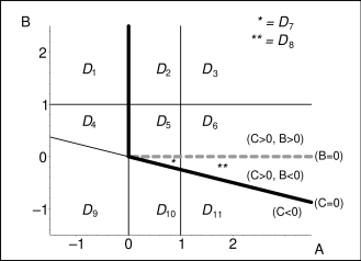
Figure 3: The $A-B$ plane of reparametrized Hamiltonian (11). After exemption of the dashed line, the points inside the thick-line-bounded upper-right wedge specify the unitary dynamical regime.

After a return to the old parameters $\alpha=\sqrt{1-A}$ and $\beta=\sqrt{1-B}$, our new $N=4$ matrix (11) would cease to be real in the whole $A-B$ plane. This slightly redefines the model. Keeping this in mind let us further recall Fig. 3 and separate the $A-B$ plane of parameters into eleven subdomains while noticing that

• in the usual matrix sense, i.e., inside the most common complex vector space ${\cal H}^{(F)}\equiv\mathbb{C}^{4}$ endowed with trivial metric $\Theta^{(F)}=I$, our (possibly, complex) Hamiltonian (11) is manifestly Hermitian just in the single subdomain ${\cal D}_{3}$;

• our four by four Hamiltonian is a real matrix with real spectrum just in the two simply connected subdomains of parameters ${\cal D}_{5}$ and ${\cal D}_{7}$;

• the spectrum is real inside the closure of the union $\overline{{\cal D}_{2}\cup{\cal D}_{3}\cup{\cal D}_{5}\cup{\cal D}_{6}\cup{\cal D}_{7}\cup{\cal D}_{8}}\,$ of six subdomains.

Figure 4: The spectrum in the vicinity of the $A=0$ horizon of the first kind.

In Fig. 3 the two thick EP half-lines with $A=0$ and $C\geq 0$ or with $C=0$ and $A\geq 0$ play the role of the boundaries of stability of the system (let us call them “quantum horizons of the first kind”). Beyond these horizons the energies complexify and cease to be observable.

The most elementary illustration of this most common form of quantum phase transition is provided by Fig. 4 where we varied parameter $A$ along a line connecting the unphysical subdomain ${\cal D}_{4}$ with its most conventional physical neighbor ${\cal D}_{5}$. Once we choose a nonvanishing second parameter $B=1/50$ we obtained a generic picture in which the two separate degenerate energies are unfolding in parallel.

With the decrease of $B>0$ the degenerate energies get closer to each other. In the limit one arrives at an exceptional, double-degeneracy scenario with $A=B=0$. The spectrum in the vicinity is sampled in Fig. 5. One moves there along the path with $B=A$ so that the system passes through the origin in a way connecting the physical region ${\cal D}_{5}$ with the twice-forbidden unphysical subdomain ${\cal D}_{9}$. Obviously, one could now reinterpret a return to the pattern of Fig. 4 as a consequence of perturbation due to which the upper and lower doublets get decoupled.

Figure 5: The confluent-EP scenario at $B=A$.

The $B=A$ pass is anomalous because inside the twice-forbidden subdomain ${\cal D}_{9}$ the model happens to have a purely imaginary spectrum. As long as this means that ${\rm Im}\ ({\rm i}\,E_{n})=0$, one could obtain a potentially measurable spectrum also in subdomain ${\cal D}_{9}$, using simply a premultiplied form $\hat{H}={\rm i}\,H^{(4)}(\alpha,\beta)$ of an after-transition candidate for one of possible physical Hamiltonians in ${\cal D}_{9}$.

4 New physics behind the unavoided level crossings

Admitting, in Fig. 3, a further decrease of $B$ below zero while keeping $A\geq 0$ we enter another dynamical regime which opens the possibility of the $C=0$ EP phase transitions of the first kind. During them one moves, typically, from the physical subdomain ${\cal D}_{7}$ to its unphysical neighbor ${\cal D}_{10}$. The parameter-dependence of the spectrum as well as its complexification pattern will be analogous to the ones displayed in Fig. 4.

Along both of the thick EP lines of Fig. 3 the phase transitions between the complex and real spectrum are qualitatively the same (i.e., in our terminology, of the first kind). In both of these cases the degeneracy of a pair of energies at the EP singularity is followed by its subsequent unfolding into unobservable complex eigenvalues. This mechanism is widely known as the so called spontaneous breakdown of ${\cal PT}$ symmetry (see also its numerous exactly solvable models in [19]).

What remains unclarified is the physical nature of the other, alternative parameter-changing processes during which a pair of energies would pass through the remaining, dashed $B=0$ EP line of Fig. 3 without getting complexified. We intend to show now that after one crosses such an EP horizon there will emerge good reasons for speaking about an anomalous phase transition “of the second kind”.

4.1 The menu of metrics

In the light of formula (8) the metric ceases to be positive definite at any EP parameter. Keeping in mind Fig. 3 we may conclude that no positive definite metric $\Theta$ can exist at $A\leq 0$, at $C\leq 0$ and at $B=0$. Temporarily, let us assume that $A>0$, $C>0$ and $B\neq 0$, therefore.

Once we insert Hamiltonian (11) in the implicit linear algebraic definition (6) of the real, symmetric and positive definite metric matrix $\Theta$, we obtain an overdetermined set of 16 equations for 10 unknown matrix elements. As long as formula (8) indicates that there are strictly four free real parameters in the family of solutions, let us pick up the quadruplet of elements $\Theta_{1j}=t_{j}$ with $j=1,2,3,4$ as free parameters. Next, let us solve the system by the standard elimination technique yielding

$$\Theta_{22}=-{\frac{-{\it{t}_{1}}+{\it{t}_{1}}\,\beta-{\it{t}_{3}}-{\it{t}_{3}}\,\alpha}{1+\beta}}\,,\ \ \ \Theta_{23}={\frac{{\it{t}_{2}}-{\it{t}_{2}}\,\alpha+{\it{t}_{4}}+{\it{t}_{4}}\,\beta}{1+\beta}}\,,\ \ \ \Theta_{24}=-{\frac{{\it{t}_{3}}\,\left(-1+\beta\right)}{1+\beta}}\,$$

in the second row of the matrix,

$$\Theta_{33}={\frac{{\it{t}_{1}}-{\it{t}_{1}}\,\alpha-{\it{t}_{1}}\,\beta+{\it{t}_{1}}\,\beta\,\alpha+{\it{t}_{3}}-{\it{t}_{3}}\,{\alpha}^{2}}{1+\beta+\alpha+\alpha\,\beta}}={\frac{\left(-{\it{t}_{1}}+{\it{t}_{1}}\,\beta-{\it{t}_{3}}-{\it{t}_{3}}\,\alpha\right)\left(-1+\alpha\right)}{\left(1+\beta\right)\left(1+\alpha\right)}}\,,$$

$$\Theta_{34}={\frac{{\it{t}_{2}}\,\left(1-\alpha-\beta+\alpha\,\beta\right)}{1+\beta+\alpha+\alpha\,\beta}}={\frac{{\it{t}_{2}}\,\left(-1+\alpha\right)\left(-1+\beta\right)}{\left(1+\beta\right)\left(1+\alpha\right)}}$$

in the third row and

$$\Theta_{44}=-{\frac{{\it{t}_{1}}\,\left(\alpha\,{\beta}^{2}-{\beta}^{2}+2\,\beta-2\,\alpha\,\beta+\alpha-1\right)}{{\beta}^{2}+\alpha\,{\beta}^{2}+2\,\beta+2\,\alpha\,\beta+1+\alpha}}=-{\frac{{\it{t}_{1}}\,\left(-1+\beta\right)^{2}\left(-1+\alpha\right)}{\left(1+\beta\right)^{2}\left(1+\alpha\right)}}$$

in the fourth row of the metric. An exhaustive, general and complete solution is obtained. It would be too space-consuming to display the whole matrix of the eligible metrics in print. Still, its display element by element enables us to discuss some of the most important consequences.

4.2 EP horizon of the second kind

The insertion of $B=0$ alias $\beta=1$ reduces our Hamiltonian (11) to one-parametric matrix

$$H=H^{(4)}(\alpha,1)=\left[\begin{array}[]{cccc}0&0&0&0\\ \vskip 6.0pt plus 2.0pt minus 2.0pt\cr-2&0&-1+\alpha&0\\ \vskip 6.0pt plus 2.0pt minus 2.0pt\cr 0&-1-\alpha&0&0\\ \vskip 6.0pt plus 2.0pt minus 2.0pt\cr 0&0&-2&0\end{array}\right]\,.$$ (14)

One can easily prove that such a matrix possesses two vanishing eigenvalues $E=0$ but just a single related eigenvector. This means that matrix (14) is non-diagonalizable and that the $B=0$ line is all composed of exceptional points. The Jordan-block canonical structure of the $B=0$ Hamiltonian cannot be Hermitized by any metric $\Theta$. Two of the eigenvectors $|\Xi_{j}\rangle$ in formula (8) coincide in the limit $B\to 0$ so that in the same limit, one of the eigenvalues of $\Theta$ goes to zero. All of the metric-candidates of the concrete form (8) become non-invertible at $B=0$.

Figure 6: The unavoided level crossing at $B=0$ for $A=1/50$.

The $B-$dependence of the energy levels is such that two of them merge at $B=0$. In the vicinity of the $B=0$ singularity (i.e., in our present terminology, along the EP horizon of the second kind) one observes the unavoided level crossing, the concrete form of which is illustrated in Fig. 6. The picture may be complemented by the closed-form construction of the bound-state solutions starting from the small-perturbation version

$$H=H^{(4)}(\alpha,1-\gamma)=\left[\begin{array}[]{cccc}0&-\gamma&0&0\\ \vskip 6.0pt plus 2.0pt minus 2.0pt\cr-2+\gamma&0&-1+\alpha&0\\ \vskip 6.0pt plus 2.0pt minus 2.0pt\cr 0&-1-\alpha&0&-\gamma\\ \vskip 6.0pt plus 2.0pt minus 2.0pt\cr 0&0&-2+\gamma&0\end{array}\right]\,$$

of the original Hamiltonian. A small shift $\gamma$ in $\beta=1-\gamma$ yields an equally small value of $B=2\gamma+{\cal O}(\gamma^{2})$ of both signs. The resulting closed form of the pair of the almost-vanishing eigenvalues reads

$$\pm 2E_{\pm,-}=\sqrt{2-2\,{\alpha}^{2}+8\,\gamma-4\,{\gamma}^{2}-2\,\sqrt{{\alpha}^{4}-8\,{\alpha}^{2}\gamma+4\,{\alpha}^{2}{\gamma}^{2}-2\,{\alpha}^{2}-4\,{\gamma}^{2}+8\,\gamma+1}}\,.$$ (15)

One quickly arrives at the required perturbation-expansion description of the crossing phenomenon in the language of Taylor series

$$E_{\pm,-}\approx\pm\left(2+{\alpha}^{2}+3/4\,{\alpha}^{4}+\ldots\right)\gamma\mp\left(5+13/2\,{\alpha}^{2}+\ldots\right){\gamma}^{2}\pm\ldots\,.$$

The change of the sign of the auxiliary small parameter $\gamma$ may be perceived as a transition between the potentially physical real-spectrum domain ${\cal D}_{5}$ and another, equally acceptable real-spectrum domain ${\cal D}_{7}$.

4.3 Phase transition of the second kind

During the above-mentioned transition, the only suspicious point is $B=0$ at which the metric ceases to exist. Hence, we have to analyze the $B-$dependence of the metric near the EP singularity at $B=0$ in a more explicit representation. Most efficiently, such a task may be simplified when we accept the specific choice of $t_{2}=t_{3}=t_{4}=0$. Under a symmetrized overall normalization choice of $t_{1}\neq 0$ this makes our metric strictly diagonal, with elements

$$\Theta_{11}={\frac{\left(1+\alpha\right)\left(1+\beta\right)}{1-\beta}}\,,\ \ \ \ \Theta_{22}=1+\alpha\,,\ \ \ \ \Theta_{33}=1-\alpha\,,\ \ \ \ \Theta_{44}={\frac{\left(1-\alpha\right)\left(1-\beta\right)}{1+\beta}}\,.$$

Inside the physical subdomain ${\cal D}_{5}$ of Fig. 3 our diagonal metric is positive definite for all of the real parameters such that $|\alpha|<1$ and $|\beta|<1$. Below the EP line $B=0$ our metric ceases to be positive definite.

As long as we stay inside the physical domain giving real energies (viz., inside subdomain ${\cal D}_{7}$ of Fig. 3) we may put $\beta=1+\delta^{2}$ (where $\delta$ is small but real) and check the statement. It gets verified: our diagonal matrix $\Theta$ loses the status of metric and becomes converted into the mere indefinite diagonal pseudometric ${\cal P}$ which possesses two negative elements and/or eigenvalues,

$${\cal P}_{11}=-{\frac{\left(1+\alpha\right)\left(2+\delta^{2}\right)}{\delta^{2}}}\,,\ \ \ \ {\cal P}_{22}=1+\alpha\,,\ \ \ \ {\cal P}_{33}=1-\alpha\,,\ \ \ \ {\cal P}_{44}=-\delta^{2}\,{\frac{1-\alpha}{2+\delta^{2}}}\,.$$

Below the EP line $B=0$, any correct physical metric must necessarily be non-diagonal. The physics of the quantum system in question will be different in the neighboring physical subdomains ${\cal D}_{5}$ and ${\cal D}_{7}$. The energies remain observable but the set of the admissible operators of observables for parameters inside ${\cal D}_{5}$ will necessarily be different from the set of the operators of observables for parameters which crossed the $B=0$ line and belong to ${\cal D}_{7}$.

Such a change of physics at $B=0$ is not as drastic as the truly catastrophic loss of the reality of the energies at the horizons $A=0$ or $C=0$. Still, one must speak about phase transition. We propose to call such a change the phase transition of the second kind.

5 Level crossings beyond $N=4$

When addressing conceptual matters we made an ample use, up to now, of the elementary nature of the toy-model secular Eq. (12) at $N=4$. At a few higher matrix dimensions $N$ the determination of the EP horizons is more complicated but still non-numerical. The methods were described in Ref. [20] where, for a not too dissimilar class of matrix models, these methods were shown effective up to $N=11$.

5.1 The family of models

The pass of a quantum observable (typically, of Hamiltonian $H(\lambda)$) through a Kato’s exceptional point $\lambda^{(EP)}$ leads, typically, to a quantum catastrophe during which certain eigenvalues collide and, subsequently, complexify. The observability status of Hamiltonian $H(\lambda)$ is lost and the critical value of $\lambda=\lambda^{(EP)}$ may be perceived as a point on horizon of quantum stability. In the alternative, eigenvalue-crossing scenario without complexification we reminded the readers that one has to distinguish between the non-EP degeneracy (typical for Hermitian models) and an anomalous, EP-caused degeneracy. In this general theoretical setting [3] we revealed that one may encounter a loss of the system’s observability implying a subtler form of the quantum phase transition.

Via the solvable $N=4$ example we discovered that the mechanism of the anomalous transition is based on the loss of the positivity of the metric at the EP singularity. The Hilbert space (i.e., its inner product, i.e., the set of the eligible operators of observales) changed. Beyond the eigenvalue-collision at $\lambda=\lambda^{(EP)}$ the physical contents of the theory may be entirely different even if the energy spectrum itself stays real.

Whenever the matrix dimensions get too large, the proofs become more and more numerical even when we keep working with the most elementary tridiagonal and finite-dimensional quasi-real matrix Hamiltonians of Ref. [18],

$$H^{(N)}({\lambda,\mu,\ldots})=\left(\begin{array}[]{ccccccc}2&-1+{\it{\lambda}}&0&\ldots&&\ldots&0\\ {}-1-{\it{\lambda}}&2&-1+{\it{\mu}}&0&\ldots&&\vdots\\ {}0&-1-{\it{\mu}}&2&-1+{\nu}&0&\ldots&\\ {}\vdots&0&-1-{\nu}&2&\ddots&\ddots&\vdots\\ {}\hfil&&\ddots&\ddots&\ddots&-1+\mu&0\\ {}\vdots&&&\ddots&-1-\mu&2&-1+{\it{\lambda}}\\ {}0&\ldots&\ldots&0&0&-1-{\it{\lambda}}&2\end{array}\right)\,.$$ (16)

The kinematics may be perceived as represented by the discrete Laplacean $T=H^{(N)}({0,0,\ldots})$. The information about the dynamics is carried by the set of $N/2$ couplings.

Our preliminary numerical experiments with the $N>4$ models of the above class proved encouraging, providing a few new qualitative insights (cf. the next subsection). On the abstract level it was useful that the interaction $V=H-T$ itself was kept minimally non-local and antisymmetric. The choice was further restricted to the matrices which were required ${\cal PT}-$symmetric with respect to the most elementary antidiagonal $N$ by $N$ parity-simulating matrix

$${\cal P}={\cal P}^{(N)}=\left[\begin{array}[]{ccccc}0&0&\ldots&0&1\\ {}0&\ldots&0&1&0\\ {}\vdots&{\large\bf{}_{.}}\cdot{\large\bf{}^{{}^{.}}}&{\large\bf{}_{.}}\cdot{\large\bf{}^{{}^{.}}}&{\large\bf{}_{.}}\cdot{\large\bf{}^{{}^{.}}}&\vdots\\ {}0&1&0&\ldots&0\\ {}1&0&\ldots&0&0\end{array}\right]\,$$ (17)

in combination with the time-reversal-simulating antilinear operator ${\cal T}$ of matrix transposition.

Figure 7: The $N=6$ spectrum near the $A=0$ horizon of the first kind.

5.2 Non-Hermitian quantum lattice with $N=6$

The study of the three-parametric $N=6$ model

$$H=H^{(6)}(\alpha,\beta.\gamma)=\left[\begin{array}[]{cccccc}0&-1+\gamma&0&0&0&0\\ \vskip 6.0pt plus 2.0pt minus 2.0pt\cr-1-\gamma&0&-1+\beta&0&0&0\\ \vskip 6.0pt plus 2.0pt minus 2.0pt\cr 0&-1-\beta&0&-1+\alpha&0&0\\ \vskip 6.0pt plus 2.0pt minus 2.0pt\cr 0&0&-1-\alpha&0&-1+\beta&0\\ \vskip 6.0pt plus 2.0pt minus 2.0pt\cr 0&0&0&-1-\beta&0&-1+\gamma\\ \vskip 6.0pt plus 2.0pt minus 2.0pt\cr 0&0&0&0&-1-\gamma&0\end{array}\right]$$ (18)

provides an insight into the pattern of possible generalizations. Reparametrizations $A=1-\alpha^{2}$, $G=1-\beta^{2}$ and $B=1-\gamma^{2}$ enable us to establish a connection between the $N=4$ and $N=6$ spectra.

Figure 8: The unavoided inner-level crossing at $B=0$ for $N=6$.

• in the “innermost coupling” dynamical regime we find the same no-intersection pattern both in Fig. 4 (where $N=4$) and in Fig. 7 (where $N=6$); the same form of the phase transition of the first kind may be expected to survive at all of the higher dimensions $N<\infty$;

• in the opposite, “outermost coupling” dynamical regime the inner-level-crossing pattern (which characterizes the phase transition of the second kind) emerges both in Fig. 6 (with $N=4$) and in Fig. 8 (with $N=6$); a very similar pattern may be expected at all $N>6$;

• in the newly emerging “intermediate-coupling” dynamical regime the phase transition of the first kind is expected; in the first nontrivial $N=6$ example of Fig. 9 the $G=0$ EP mergers only involve two pairs of levels while the reality of the remaining spectrum is not destroyed. This or similar pattern is also expected to occur at $N>6$.

Figure 9: The $N=6$ spectrum near the $B=0$ horizon of the first kind.

6 Conclusions

Let us summarize that in applications of quantum theory the specification of the physical domain ${\cal D}$ of parameters may be understood in two ways. A parameter may vary in Hamiltonian $H=H(\lambda)$ itself (plus, naturally, in the related physical Hilbert-space metric) or solely in the physical Hilbert space metric (remember that the choice of the Hamiltonian-Hermitizing metric $\Theta=\Theta(\lambda,\kappa)$ is not unique in general [12]).

In the former case people often assume that the pass of the quantum system in question through the EP boundary $\partial{\cal D}$ leads to the complexification of some energies so that the unitarity of the evolution is inadvertently lost. In our present paper we considered the second possibility in which the pass through the EP boundary does not destroy the reality of the energies.

We imagined that in such a case one must ask the following natural question: “Does this imply that the unitarity of the evolution is preserved?” A nontriviality of this question lies in the fact that after the pass through EP, the very definition of the norm of the wave functions may change.

By means of a constructive analysis of a few solvable models we managed to demonstrate that in some cases when boundary merely separates two disjoint physical subdomains ${\cal D}_{\pm}$ the change of the definition of the norm of the wave functions is unavoidable. The value of the norm of a given wave function performs, in general, a jump when crossing such an EP horizon $\partial{\cal D}$ of the second kind. In such a dynamical scenario it is necessary to speak about a phase transition of the second kind.

We described the mechanism in more detail. Keeping in mind the popularity of the phase transition of the first kind (during which the change of the metric is accompanied by the necessary change of the effective Hamiltonian) we emphasized the contrast. We introduced the concept of the phase transition of the second kind during which the change of the metric is not accompanied by any change of the effective Hamiltonian. Subsequently we emphasized that the change of the physics is subtler, mediated merely by the change of the physical Hilbert space, with all of its well known consequences for non-Hamiltonian observables.

In the related literature one often finds the phase transition of the first kind interpreted as a symptom of a spontaneous breakdown of the ${\cal PT}$ symmetry of the system [1]. Via our illustrative examples we demonstrated that the spontaneous breakdown of the ${\cal PT}$ symmetry is not necessary for the existence of quantum phase transition. A “no-complexification” dynamical scenario may exist during which the phase transition does not require any lasting loss of ${\cal PT}$ symmetry.

The possibility seems anomalous because after the system passes through the singularity $\lambda^{(EP)}$, the Hamiltonian survives without any changes. The most amazing consequence of the phase transition of the second kind may be seen in the loss of the observability status of multiple operators of observables. The crypto-Hermiticity of many of them will only hold before or after the transition. In any case, the occurrence of the phase transition of both kinds will change the physics thoroughly.

Acknowledgements

D.B. was partially supported by grant of RFBR, grant of President of Russia for young scientists-doctors of sciences (MD-183.2014.1) and Dynasty fellowship for young Russian mathematicians. M.Z. was supported by RV O61389005.

References

- [1] C. M. Bender, Rep. Prog. Phys. 70 (2007) 947.
- [2] Z. Ahmed, D. Ghosh, J. A. Nathan and G. Parkar, Phys. Lett. A 379 (2015) 2424; M. Znojil, arXiv:1303.4876 (unpublished).
- [3] D. I. Borisov, Acta Polytech. 54 (2014) 93 (arXiv:1401.6316).
- [4] M. Znojil, Phys. Lett. A 259 (1999) 220.
- [5] T. Kato, Perturbation theory for linear operators, Springer-Verlag, Berlin, 1966.
- [6] M. Znojil, J. Phys. A: Math. Theor. 45 (2012) 444036; Y. N. Joglekar, C. Thompson, D. D. Scott and G. Vemuri, Eur. Phys. J. Appl. Phys. 63 (2013) 30001; D. E. Pelinovsky, P. G. Keverekidis and D. J. Frantzeskakis, Eur. Phys. Lett. 101 (2013) 11002; C. H. Liang, D. D. Scott and Y. N. Joglekar, Phys. Rev. A 89 (2014) 030102(R); D. I. Borisov, F. Ruzicka and M. Znojil, Int. J. Theor. Phys., in print, http://dx.doi.org/10.1007/s10773-014-2493-y (arXiv:1412.6634).
- [7] M. Znojil, J. Phys. A: Math. Theor. 40 (2007) 4863; M. Znojil, J. Phys. A: Math. Theor. 40 (2007) 13131.
- [8] A. Mostafazadeh, J. Phys. A: Math. Gen. 39 (2006) 10171; C. F. de Morison Faria and A, Fring, Czech. J. Phys. 56 (2006) 899; V. Jakubsky and J. Smejkal, Czech. J. Phys. 56 (2006) 985; A. Ghatak and B. P. Mandal, Comm. Theor. Phys. 59 (2013) 553.
- [9] D. Krejčiřík, P. Siegl and J. Železný, Complex Anal. Oper. Theory 8 (2014) 255; D. C. Brody, Consistency of PT-symmetric quantum mechanics, arXiv: 1508.02190.
- [10] D. Krejčiřík and P. Siegl, J. Phys. A: Math. Theor. 43 (2010) 485204; F. Bagarello and M. Znojil, J. Phys. A: Math. Theor. 44 (2011) 415305; D. Borisov and D. Krejcirik, Asympt. Anal. 76 (2012) 49.
- [11] M. Znojil, SIGMA 5 (2009) 001 (arXiv overlay: 0901.0700); M. Znojil, Int. J. Theor. Phys. 52 (2013) 2038.
- [12] F. G. Scholtz, H. B. Geyer and F. J. W. Hahne, Ann. Phys. (NY) 213 (1992) 74.
- [13] M. Znojil and H. B. Geyer, Fort. d. Physik 61 (2013) 111.
- [14] A. Mostafazadeh, Int. J. Geom. Meth. Mod. Phys. 7 (2010) 1191
- [15] M. Znojil, SIGMA 4 (2008) 001 (arXiv overlay: 0710.4432).
- [16] M. Znojil, in “Non-Selfadjoint Operators in Quantum Physics: Mathematical Aspects”, F. Bagarello et al, Eds, Wiley, Hoboken, 2015, pp. 7 - 58.
- [17] D. Krejčiřík, H. Bíla and M. Znojil, J. Phys. A 39 (2006) 10143; D. Krejčiřík, J. Phys. A: Math. Theor. 41 (2008), 244012; C. M. Bender, K. Besseghir, H. F. Jones, and X. Yin, J. Phys. A: Math. Theor. 42 (2009), 355301.
- [18] M. Znojil and J. Wu, Int. J. Theor. Phys. 52 (2013) 2152.
- [19] G. Levai and M. Znojil, Mod. Phys. Lett. A 16 (2001) 1973; A. Sinha and P. Roy, J. Phys. A: Math. Gen. 39 (2006) L377; P. Dorey, C. Dunning, A. Lishman and R. Tateo, J. Phys. A: Math. Theor. 42 (2009) 465302; G. Levai, J. Phys. A: Math. Theor. 45 (2012) 444020.
- [20] M. Znojil, J. Phys. A: Math. Theor. 41 (2008) 244027.