Estimation of the lead-lag parameter from non-synchronous data

Abstract

We propose a simple continuous time model for modeling the lead-lag effect between two financial assets. A two-dimensional process $(X_{t},Y_{t})$ reproduces a lead-lag effect if, for some time shift $\vartheta\in\mathbb{R}$, the process $(X_{t},Y_{t+\vartheta})$ is a semi-martingale with respect to a certain filtration. The value of the time shift $\vartheta$ is the lead-lag parameter. Depending on the underlying filtration, the standard no-arbitrage case is obtained for $\vartheta=0$. We study the problem of estimating the unknown parameter $\vartheta\in\mathbb{R}$, given randomly sampled non-synchronous data from $(X_{t})$ and $(Y_{t})$. By applying a certain contrast optimization based on a modified version of the Hayashi–Yoshida covariation estimator, we obtain a consistent estimator of the lead-lag parameter, together with an explicit rate of convergence governed by the sparsity of the sampling design.

, and

1 Introduction

Market participants usually agree that certain pairs of assets $(X,Y)$ share a “lead-lag effect,” in the sense that the lagger (or follower) price process $Y$ tends to partially reproduce the oscillations of the leader (or driver) price process $X$, with some temporal delay, or vice-versa. This property is usually referred to as the “lead-lag effect.” The lead-lag effect may have some importance in practice, when assessing the quality of risk management indicators, for instance, or, more generally, when considering statistical arbitrage strategies. Also, note that it can be measured at various temporal scales (daily, hourly or even at the level of seconds, for flow products traded on electronic markets).

The lead-lag effect is a concept of common practice that has some history in financial econometrics. In time series for instance, this notion can be linked to the concept of Granger causality, and we refer to Comte and Renault [4] for a general approach. From a phenomenological perspective, the lead-lag effect is supported by empirical evidence reported in [6, 3] and [18], together with [20] and the references therein. To our knowledge, however, only few mathematical results are available from the point of view of statistical estimation from discretely observed, continuous-time processes. The purpose of this paper is to – partly – fill in this gap. (Also, recently, Robert and Rosenbaum study in [23] the lead-lag effect by means of random matrices, in a mixed asymptotic framework, a setting which is relatively different than in the present paper.)

1.1 Motivation

(

• 1)]

• Our primary goal is to provide a simple – yet relatively general – model for capturing the lead-lag effect in continuous time, readily compatible with stochastic calculus in financial modeling. Informally, if $\tau_{-\vartheta}(Y)_{t}:=Y_{t+\vartheta}$, with $\vartheta\in\mathbb{R}$, is the time-shift operator, we say that the pair $(X,Y)$ will produce a lead-lag effect as soon as $(X,\tau_{-\vartheta}(Y))$ is a (regular) semi-martingale with respect to an appropriate filtration, for some $\vartheta$, called the lead-lag parameter. The usual no-arbitrage case is embedded into this framework for $\vartheta=0$. More in Section 2 below.

• At a similar level of importance, we aim at constructing a simple and efficient procedure for estimating the lead-lag parameter $\vartheta$ based on historical data. The underlying statistical model is generated by a – possibly random – sampling of both $X$ and $Y$. The sampling typically happens at irregularly and non-synchronous times for $X$ and $Y$. We construct, in the paper, an estimator of $\vartheta$ based on a modification of the Hayashi–Yoshida covariation estimator; see [11] and [13]. Our result is that the lead-lag parameter can be consistently estimated against a fairly general class of sampling schemes. Moreover, we explicit the rate of convergence of our procedure.

• From a financial point of view, unless appropriate time shifts are operated, our model incapacitates our primary assets $X$ and $Y$ to be a semi-martingale with respect to the same filtration. This is consistent, as far as modeling is concerned, but allows, in principle, for market imperfections such as statistical arbitrage if the lead-lag parameter $\vartheta$ is different from zero. More in Section 3.4 below. Addressing such a possibility is indeed the issue of the lead-lag effect, but we will content ourselves with detecting whether the lead-lag effect is present or not. The quantization of statistical arbitrage in terms of $\vartheta$ (and other parameters such as trading frequency, market friction, volatility and so on) lies beyond the scope of this paper.

• From a statistical inference point of view, the statistician and the data provider are not necessarily the same agents, and this leads to technical difficulties linked to the sampling strategy. The data provider may choose the opening/closing for $X$ and $Y$, possibly traded on different markets, possibly on different time clocks. He or she may also sample points at certain trading times or events which are randomly chosen in a particular time window. This typically happens if daily data are considered. At a completely different level, if high-frequency data are concerned, trading times are genuinely random and non-synchronous. Our approach will simultaneously incorporate these different points of view.

1.2 Organization of the paper

In Section 2, we present our stochastic model for describing the lead-lag effect. We start with the simplest Bachelier model with no drift in Section 2.1. The issue boils down to defining properly the lead-lag effect between two correlated Brownian motions. In Section 2.2, a general lead-lag model is presented for two-dimensional process, for which the marginal processes are semi-martingales with locally bounded drift and continuous local martingale part, with properly defined diffusion coefficients.

We present our main result in Section 3. Section 3.1 gives a precise construction of the underlying statistical experiment with the corresponding assumptions on the observation sampling schemes. The estimation procedure is constructed in Section 3.2, via an appropriate contrast function based on the covariation between $X$ and $Y$ when one asset is artificially shifted in time, the amount of this shift being the argument of the contrast function. Our estimator is robust to non-synchronous data and does not require any pre-processing contrary to the previous tick algorithm; see, for example, [27]. In Section 3.3, we state our main result in Theorem 1: we show that the lead-lag parameter between $X$ and $Y$ can be consistently estimated from non-synchronous historical data over a fixed time horizon $[0,T]$. The rate is governed by $\Delta_{n}$, the maximal distance between two data points. We show that the rate of convergence of our estimator is essentially $\Delta_{n}^{-1}$ and not $\Delta_{n}^{-1/2}$, as one would expect from a regular estimation problem in diffusion processes; see, for example, [7]. This comes from the underlying structure of the statistical model, which is not regular, and which shares some analogy with change-point problems. As for our procedure, we investigate further its asymptotic properties in Proposition 1 when we confine ourselves to the simpler case where $X$ and $Y$ are marginally Brownian motions that are observed at synchronous data points. In that case, we can exhibit a central limit theorem for our contrast function. A closer inspection of the limiting variance reveals the effect of the correlation between the two assets, which also plays a role in the accuracy of the estimation procedure. Finally, we show in Proposition 2 that a simple central limit theorem cannot hold for our estimator. We discuss this effect which is somewhat linked to the discretisation of our method.

Theorem 1 is good news, as far as practical implementation is concerned, and is further addressed in the discussion in Section 3.4, appended with numerical illustrations on simulated data in Section 5 and on real data in Section 6. The proofs are delayed until Section 4 and the Appendix contains auxiliary technical results.

2 The lead-lag model

2.1 The Bachelier model

A simple lead-lag Bachelier model with no drift between two Brownian motion components can be described as follows. On a filtered space $(\Omega,{\mathcal{F}},\mathbb{F}=({\mathcal{F}}_{t})_{t\geq 0},\mathbb{P})$, we consider a two-dimensional $\mathbb{F}$-Brownian motion $B=(B^{(1)},B^{(2)})$ such that $\langle B^{(1)},B^{(2)}\rangle_{t}=\rho t$ for every $t\geq 0$ and for some $\rho\in[-1,1]$. Let $T>0$ be some terminal time, fixed throughout the paper. For $t\in[0,T]$, set

$$\cases{X_{t}:=x_{0}+\sigma_{1}B^{(1)}_{t},\vspace*{2pt}\cr\widetilde{Y}_{t}:=y_{0}+\sigma_{2}B^{(2)}_{t},}$$

where $x_{0},y_{0}\in\mathbb{R}$ and $\sigma_{1}>0$, $\sigma_{2}>0$ are given constants. The corresponding Black–Scholes version of this model is readily obtained by exponentiating $X$ and $\widetilde{Y}$. We introduce a lead-lag effect between $X$ and $\widetilde{Y}$ by operating a time shift: let $\vartheta\in\mathbb{R}$ represent the lead or lag time between $X$ and $\widetilde{Y}$ (and assume for simplicity that $\vartheta\geq 0$). Put

$$\tau_{\vartheta}(\widetilde{Y})_{t}:=\widetilde{Y}_{t-\vartheta},\qquad t\in[\vartheta,T].$$ (1)

Our lead-lag model is the two-dimensional process

$$(X,\tau_{\vartheta}(\widetilde{Y}))=(X_{t},\tau_{\vartheta}(\widetilde{Y})_{t})_{t\in[\vartheta,T]}.$$

Since we have $B^{(2)}_{t}=\rho B^{(1)}_{t}+(1-\rho^{2})^{1/2}W_{t}$ with $W=(W_{t})_{t\in[0,T]}$, a Brownian motion independent of $B^{(1)}$, we obtain the simple and explicit representation

$$\cases{X_{t}=x_{0}+\sigma_{1}B^{(1)}_{t},\vspace*{2pt}\cr\tau_{\vartheta}(\widetilde{Y})_{t}=y_{0}+\rho\sigma_{2}B^{(1)}_{t-\vartheta}+\sigma_{2}(1-\rho^{2})^{1/2}W_{t-\vartheta}}$$ (2)

for $t\in[\vartheta,T]$. In this representation, the interpretation of the lead-lag parameter $\vartheta$ is transparent. Alternatively, if we start with a process $(X,Y)$ having representation

$$(X,Y)=(X,\tau_{\vartheta}(\widetilde{Y}))$$ (3)

as in (2), the lead-lag interpretation between $X$ and $Y$ readily follows. Since $\vartheta\geq 0$, the sample path of $X$ anticipates on the path of $Y$ by a time shift $\vartheta$ and to an amount – measured in normalized standard deviation – proportional to $\rho\sigma_{2}/\sigma_{1}$. In that case, we say that $X$ is the leader, and $Y$ is the lagger. For the case $\vartheta<0$, we intertwine the roles of $X$ and $Y$ in the terminology.

Remark 0.

Note that, except in the case $\vartheta=0$, the process $(X_{t},Y_{t})_{t\in[\vartheta,T]}$ is not an $\mathbb{F}$-martingale. However, each component is a martingale with respect to a different filtration: $X$ is an $\mathbb{F}$-martingale and $Y=\tau_{\vartheta}(\widetilde{Y})$ is an $\mathbb{F}^{\vartheta}$-martingale, with $\mathbb{F}^{\vartheta}=(\mathcal{F}^{\vartheta}_{t})_{t\geq\vartheta}$, and $\mathcal{F}^{\vartheta}_{t}=\mathcal{F}_{t-\vartheta}$.

2.2 Lead-lag between two semi-martingales

We generalize the lead-lag model (3) to semi-martingales with local martingale components that can be represented as Itô local martingales.

We need some notation. Let $T>0$ be some terminal time, and let $\delta>0$ represent the maximum temporal lead-lag allowed for the model, fixed throughout the paper. On a probability space $(\Omega,{\mathcal{F}},\mathbb{P})$, let $\mathbb{F}=({\mathcal{F}}_{t})_{t\in[-\delta,T+\delta]}$ be a filtration satisfying the usual conditions. We denote by $\mathbb{F}_{[a,b]}=({\mathcal{F}}_{t})_{t\in[a,b]}$ the restriction of $\mathbb{F}$ to the time interval $[a,b]$.

Definition 1.

The two-dimensional process $(X,Y)_{t\in[0,T+\delta]}$ is a regular semi-martingale with lead-lag parameter $\vartheta\in[0,\delta)$ if the following decomposition holds:

$$X=X^{c}+A,\qquad Y=Y^{c}+B,$$

with the following properties:

• The process $(X^{c}_{t})_{t\in[0,T+\delta]}$ is a continuous $\mathbb{F}_{[0,T+\delta]}$-local martingale, and the process $(Y^{c}_{t})_{t\in[0,T+\delta]}$ is a continuous $\mathbb{F}^{\vartheta}_{[0,T+\delta]}$-local martingale.

• The quadratic variations $\langle X^{c}\rangle_{t\in[0,T+\delta]}$ and $\langle Y^{c}\rangle_{t\in[0,T+\delta]}$ are absolutely continuous w.r.t. the Lebesgue measure, and their Radon–Nikodym derivatives admit a locally bounded version.

• The drifts $A$ and $B$ have finite variation over $[0,T+\delta]$.

Definition 2.

The two-dimensional process $(X,Y)_{t\in[0,T+\delta]}$ is a regular semi-martingale with lead-lag parameter $\vartheta\in(-\delta,0]$ if the same properties as in Definition 1 hold, with $X$ and $Y$ intertwined and $\vartheta$ replaced by $-\vartheta$.

Remark 0.

If $(X,Y)_{t\in[0,T+\delta]}$ is a regular semi-martingale with lead-lag parameter $\vartheta\in[0,\delta)$, then the process $(\tau_{-\vartheta}(Y^{c}))_{t\in[-\vartheta,T]}$ is a continuous $\mathbb{F}_{[-\vartheta,T]}$-local martingale, with $\tau_{-\vartheta}(Y)_{t}=Y_{t+\vartheta}$ the (inverse of the) shift operator defined in (1).

Remark 0.

If $(X,Y)_{t\in[0,T+\delta]}$ is a regular semi-martingale with lead-lag parameter $\vartheta\in[0,\delta)$, then the process $(Y,X)_{t\in[0,T+\delta]}$ is a regular semi-martingale with lead-lag parameter $-\vartheta$.

3 Main result

3.1 The statistical model

We observe a two-dimensional price process $(X,Y)$ at discrete times. The components $X$ and $Y$ are observed over the time horizon $[0,T+\delta]$. The following assumption is in force throughout:

Assumption A.

The process $(X,Y)=(X_{t},Y_{t})_{t\in[0,T+\delta]}$ is a regular semi-martingale with lead-lag parameter $\Theta\in\vartheta=(-\delta,\delta)$.

The – possibly random – observation times are given by the following subdivisions of $[0,T+\delta]$:

$${\mathcal{T}}^{X}:=\{s_{1,n_{1}}<s_{2,n_{1}}<\cdots<s_{n_{1},n_{1}}\}$$ (4)

for $X$ and

$${\mathcal{T}}^{Y}:=\{t_{1,n_{2}}<t_{2,n_{2}}<\cdots<t_{n_{2},n_{2}}\}$$ (5)

for $Y$, with $n_{1}=n_{2}$ or not. For simplicity, we assume $s_{1,n_{1}}=t_{1,n_{2}}=0$ and $s_{n_{1},n_{1}}=t_{n_{2},n_{2}}=T+\delta$. The sample points are either chosen by the statistician or dictated for practical convenience by the data provider. They are usually neither equispaced in time nor synchronous, and may depend on the values of $X$ and $Y$.

For some unknown $\vartheta\in\Theta:=(-\delta,\delta)$, the process $(X,Y)$ is a regular semi-martingale with lead-lag parameter $\vartheta$, and we want to estimate $\vartheta$ based on the set of historical data

$$\{X_{s},s\in{\mathcal{T}}^{X}\}\cup\{Y_{t},t\in{\mathcal{T}}^{Y}\}.$$ (6)

In order to describe precisely the property of the sampling scheme ${\mathcal{T}}^{X}\cup{\mathcal{T}}^{Y}$, we need some notation that we borrow from Hayashi and Yoshida [11]. The subdivision ${\mathcal{T}}^{X}$ introduced in (4) is mapped into a family of intervals

$${\mathcal{I}}=\{I=(\underline{I},\overline{I}]=(s_{i,n_{1}},s_{i+1,n_{1}}],i=1,\ldots,n_{1}-1\}.$$ (7)

Likewise, the subdivision ${\mathcal{T}}^{Y}$ defined in (5) is mapped into

$${\mathcal{J}}=\{J=(\underline{J},\overline{J}]=(t_{j,n_{2}},s_{j+1,n_{2}}],j=1,\ldots,n_{2}-1\}.$$

We will systematically employ the notation $I$ (resp., $J$) for an element of ${\mathcal{I}}$ (resp., ${\mathcal{J}}$). We set

$$\Delta_{n}:=\max\bigl{\{}\sup\{|I|,I\in{\mathcal{I}}\},\sup\{|J|,J\in{\mathcal{J}}\}\bigr{\}},$$

where $|I|$ (resp., $|J|$) denotes the length of the interval $I$ (resp., $J$), and $n$ is a parameter tending to infinity.

Remark 0.

One may think of $n$ being the number of data points extracted from the sampling, that is, $n=\sharp{\mathcal{I}}+\sharp{\mathcal{J}}$. However, as we will see, only the (random) quantity $\Delta_{n}$ will prove relevant for measuring the accuracy of estimation of the lead-lag parameter.

The assumptions on the sampling scheme is the following.

Assumption B.

1. [B1.]

2. There exists a deterministic sequence of positive numbers $v_{n}$ such that $v_{n}<\delta$ and $v_{n}\rightarrow 0$ as $n\rightarrow\infty$. Moreover

   $$v_{n}^{-1}\Delta_{n}\rightarrow 0$$

   in probability as $n\rightarrow\infty$.

3. For all $I\in{\mathcal{I}}$, the random times $\underline{I}$ and $\overline{I}$ are $\mathbb{F}^{v_{n}}$-stopping times if $\vartheta\geq 0$ (resp., $\mathbb{F}^{-\vartheta+v_{n}}$-stopping times if $\vartheta<0$). For all $J\in{\mathcal{J}}$, the random times $\underline{J}$ and $\overline{J}$ are $\mathbb{F}^{\vartheta+v_{n}}$-stopping times if $\vartheta\geq 0$ (resp., $\mathbb{F}^{v_{n}}$-stopping times if $\vartheta<0$).

4. There exists a finite grid ${\mathcal{G}}^{n}\subset\Theta$ such that $0\in{\mathcal{G}}^{n}$ and

   • [–]

   • For some $\gamma>0$, we have $\sharp{\mathcal{G}}^{n}=\mathrm{O}(v_{n}^{-\gamma})$.

   • For some deterministic sequence $\rho_{n}>0$, we have

     $$\bigcup_{\widetilde{\vartheta}\in{\mathcal{G}}^{n}}[\widetilde{\vartheta}-\rho_{n},\widetilde{\vartheta}+\rho_{n}]\supset\Theta$$

     and

     $$\lim_{n\rightarrow\infty}\rho_{n}\min\{\mathbb{E}[\sharp{\mathcal{I}}],\mathbb{E}[\sharp{\mathcal{J}}]\}\rightarrow 0.$$

Remark 0.

Since both $\mathbb{E}[\sharp{\mathcal{I}}]$ and $\mathbb{E}[\sharp{\mathcal{J}}]$ diverge at rate no less than $v_{n}^{-1}$, Assumption B3 implies that $\rho_{n}=\mathrm{o}(v_{n})$. With no loss of generality, we thus may (and will) assume that $\rho_{n}\leq v_{n}$ for all $n$.

3.2 The estimation procedure

Preliminaries

Assume first that the data arrive at regular and synchronous time stamps over the time interval $[0,T]=[0,1]$, with $\Delta_{n}=1/n$ for simplicity. This means that we have $2n+2$ observations

$$(X_{0},Y_{0}),(X_{1/n},Y_{1/n}),(X_{2/n},Y_{2/n}),\ldots,(X_{1},Y_{1}).$$

For every integer $k\in\mathbb{Z}$, we form the shifted time series

$$Y_{(k+i)/n},\qquad i=1,2,\ldots$$

for every $i$ such that $(k+i)/n$ is an admissible time stamp. We can then construct the empirical covariation estimator

$${\mathcal{C}}_{n}(k):=\sum_{i}\bigl{(}X_{i/n}-X_{(i-1)/n}\bigr{)}\bigl{(}Y_{(i+k)/n}-Y_{(i+k-1)/n}\bigr{)},$$

where the sum in $i$ expands over all relevant data points. Over the time interval $[0,1]$, the number of elements used for the computation of ${\mathcal{C}}_{n}(k)$ should be of order $n$ as $n\rightarrow\infty$. Assume further for simplicity that the process $(X,Y)$ is a lead-lag Bachelier model in the sense of Section 2.1, with lead-lag parameter $\vartheta=\vartheta_{n}=k^{0}_{n}/n$, with $k^{0}_{n}$ an integer. On the one hand, for $k=k^{0}_{n}$, we have the decomposition

$${\mathcal{C}}_{n}(k^{0}_{n})=T_{n}^{(1)}+T_{n}^{(2)},$$

with

$$T_{n}^{(1)} = \rho\sigma_{1}\sigma_{2}\sum_{i}\bigl{(}B^{(1)}_{i/n}-B^{(1)}_{(i-1)/n}\bigr{)}^{2},$$

$$T_{n}^{(2)} = \sqrt{1-\rho^{2}}\sigma_{1}\sigma_{2}\sum_{i}\bigl{(}B^{(1)}_{i/n}-B^{(1)}_{(i-1)/n}\bigr{)}\bigl{(}W_{i/n}-W_{(i-1)/n}\bigr{)}.$$

Computing successively the fourth-order moment of the random variables $T_{n}^{(1)}-\rho\sigma_{1}\sigma_{2}$ and $T_{n}^{(2)}$ and applying Markov’s inequality and the Borel–Cantelli lemma, elementary computations show that $T_{n}^{(1)}\rightarrow\rho\sigma_{1}\sigma_{2}$ and $T_{n}^{(2)}\rightarrow 0$ as $n\rightarrow\infty$ almost surely, and we derive

$${\mathcal{C}}_{n}(k^{0}_{n})\rightarrow\rho\sigma_{1}\sigma_{2}\qquad\mbox{as }n\rightarrow\infty\mbox{ almost surely}.$$

On the other hand, for $k\neq k^{0}_{n}$, we have

$${\mathcal{C}}_{n}(k)=\widetilde{T}_{n}^{(1)}+\widetilde{T}_{n}^{(2)},$$

with

$$\widetilde{T}_{n}^{(1)} = \rho\sigma_{1}\sigma_{2}\sum_{i}\bigl{(}B^{(1)}_{i/n}-B^{(1)}_{(i-1)/n}\bigr{)}\bigl{(}B^{(1)}_{(i+k-k^{0}_{n})/n}-B^{(1)}_{(i+k-k^{0}_{n}-1)/n}\bigr{)},$$

$$\widetilde{T}_{n}^{(2)} = \sqrt{1-\rho^{2}}\sigma_{1}\sigma_{2}\sum_{i}\bigl{(}B^{(1)}_{i/n}-B^{(1)}_{(i-1)/n}\bigr{)}\bigl{(}W_{(i+k-k^{0}_{n})/n}-W_{(i+k-k^{0}_{n}-1)/n}\bigr{)}.$$

Thus, for fixed $n$ and $k>k^{0}_{n}$, the process

$$j\leadsto\sum_{i=1}^{j}\bigl{(}X_{i/n}-X_{(i-1)/n}\bigr{)}\bigl{(}Y_{(i+k)/n}-Y_{(i+k-1)/n}\bigr{)}$$

is $(\mathcal{F}_{(j+k-k^{0}_{n})/n})_{j\geq 1}$-martingale. Consequently, using the Burkholder–Davis–Gundy inequality, we easily obtain that

$$\mathbb{E}[{\mathcal{C}}_{n}(k)^{6}]\leq cn^{-3},$$

up to some constant $c>0$. The same result holds for $k<k^{0}_{n}$. We infer

$$\mathbb{E}\Bigl{[}\Bigl{(}\mathop{\operatorname{sup}}_{k\neq k^{0}_{n}}|{\mathcal{C}}_{n}(k)|\Bigr{)}^{6}\Bigr{]}\leq cn^{-2}$$

up to a modification of $c$. Using again Markov’s inequality and the Borel–Cantelli lemma, we finally obtain that

$$\mathop{\operatorname{sup}}_{k\neq k^{0}_{n}}|{\mathcal{C}}_{n}(k)|\rightarrow 0\qquad\mbox{as }n\rightarrow\infty\mbox{ almost surely}.$$

Therefore, provided $\rho\sigma_{1}\sigma_{2}\neq 0$, we can detect asymptotically the value $k^{0}_{n}$ that defines $\vartheta$ in the very special case $\vartheta=k^{0}_{n}\Delta_{n}$, using $\widehat{k^{0}_{n}}$ defined as one maximizer in $k$ of the contrast sequence

$$k\leadsto|{\mathcal{C}}_{n}(k)|.$$

Indeed, from the preceding computations, we have

$$\mbox{Almost surely, for large enough }n,\qquad\widehat{k^{0}_{n}}=k^{0}_{n}.$$ (8)

This is the essence of our method. For an arbitrary $\vartheta$, we can anticipate that an approximation of $\vartheta$ taking the form $k^{0}_{n}\Delta_{n}$ would add an extra error term of the order of the approximation, that is, $\Delta_{n}$, which is a first guess for an achievable rate of convergence.

In a general context of regular semi-martingales with lead-lag effect, sampled at random non-synchronous data points, we consider the Hayashi–Yoshida (later abbreviated by HY) covariation estimator and modify it with an appropriate time shift on one component. We maximize the resulting empirical covariation estimator with respect to the time shift over an appropriate grid.

Construction of the estimator

We need some notation. If $H=(\underline{H},\overline{H}]$ is an interval, for $\vartheta\in\Theta$, we define the shift interval $H_{\vartheta}:=H+\vartheta=(\underline{H}+\vartheta,\overline{H}+\vartheta]$. We write

$$X(H)_{t}:=\int_{0}^{t}1_{H}(s)\,\mathrm{d}X_{s}$$

for a (possibly random) interval, such that $s\leadsto 1_{H}(s)$ is an elementary predictable process. Also, for notational simplicity, we will often use the abbreviation

$$X(H):=X(H)_{T+\delta}=\int_{0}^{T+\delta}1_{H}(s)\,\mathrm{d}X_{s}.$$

The shifted HY covariation contrast is defined as the function

$$\tilde{\vartheta} \leadsto {\mathcal{U}}^{n}(\tilde{\vartheta})$$

$$:= 1_{\tilde{\vartheta}\geq 0}\sum_{I\in{\mathcal{I}},J\in{\mathcal{J}},\overline{I}\leq T}X(I)Y(J)1_{\{I\cap J_{-\tilde{\vartheta}}\neq\varnothing\}}$$

$${}+1_{\tilde{\vartheta}<0}\sum_{I\in{\mathcal{I}},J\in{\mathcal{J}},\overline{J}\leq T}X(I)Y(J)1_{\{J\cap I_{\tilde{\vartheta}}\neq\varnothing\}}.$$

Our estimator $\widehat{\vartheta}_{n}$ is obtained by maximizing the contrast $\tilde{\vartheta}\leadsto|{\mathcal{U}}^{n}(\tilde{\vartheta})|$ over the finite grid ${\mathcal{G}}^{n}$ constructed in Assumption B3 in Section 3.1 above. Eventually, $\widehat{\vartheta}_{n}$ is defined as a solution of

$$|{\mathcal{U}}^{n}(\widehat{\vartheta}_{n})|=\max_{\tilde{\vartheta}\in{\mathcal{G}}^{n}}|{\mathcal{U}}^{n}(\tilde{\vartheta})|.$$ (9)

3.3 Convergence results

Since $\tau_{-\vartheta}(Y^{c})$ is a $\mathbb{F}$-local martingale, the quadratic variation process $\langle X^{c},\tau_{-\vartheta}(Y^{c})\rangle$ is well defined. We are now ready to assess our main result:

Theorem 1

Work under Assumptions A and B. The estimator $\widehat{\vartheta}_{n}$ defined in (9) satisfies

$$v_{n}^{-1}(\widehat{\vartheta}_{n}-\vartheta)\rightarrow 0$$

in probability, on the event $\{\langle X^{c},\tau_{-\vartheta}(Y^{c})\rangle_{T}\neq 0\}$, as $n\rightarrow\infty$.

Theorem 1 provides a rate of convergence for our estimator: the accuracy $\Delta_{n}^{-1}$ is nearly achievable, to within arbitrary accuracy. The next logical step is the availability of a central limit theorem. In the general case, this is not straightforward. We may, however, be more accurate if we further restrict ourselves to synchronous data in the Bachelier case; that is, we have data

$$(X_{0},Y_{0}),(X_{\Delta_{n}},Y_{\Delta_{n}}),(X_{2\Delta_{n}},Y_{2\Delta_{n}}),\ldots$$ (10)

over the time interval $[0,T]$, and the process $(X,Y)$ admits representation (3). We can then exhibit the asymptotic behavior of the contrast function $\vartheta\leadsto{\mathcal{U}}^{n}(\vartheta)$, in a vicinity of size $\Delta_{n}$, of the lead-lag parameter. More precisely, we have the following proposition.

Proposition 1.

Let $\varphi(t)=(1-|t|)1_{|t|\leq 1}$ denote the usual hat function. Let us consider the Bachelier model (3) and a synchonous observation sampling scheme (10), with lead-lag parameter $\vartheta\in\Theta$. If $|\tilde{\vartheta}-\vartheta|\leq\Delta_{n}$, we have

$${\mathcal{U}}^{n}(\tilde{\vartheta})=\sigma_{1}\sigma_{2}\bigl{(}T\rho\varphi\bigl{(}\Delta_{n}^{-1}(\tilde{\vartheta}-\vartheta)\bigr{)}+T^{1/2}\Delta_{n}^{1/2}\sqrt{1+\rho^{2}\varphi\bigl{(}\Delta_{n}^{-1}(\tilde{\vartheta}-\vartheta)\bigr{)}}\xi^{n}\bigr{)},$$

where $\xi^{n}$ is a sequence of random variables that converge in distribution to the standard Gaussian law ${\mathcal{N}}(0,1)$ as $n\rightarrow\infty$.

This representation is useful to understand the behavior of the contrast function ${\mathcal{U}}_{n}(\tilde{\vartheta})$: up to a scaling factor, $|{\mathcal{U}}^{n}(\tilde{\vartheta})|$ is asymptotically proportional to the realization of the absolute value of Gaussian random variable $|{\mathcal{N}}(m_{n}(\tilde{\vartheta}),a_{n}(\tilde{\vartheta})^{2})|$, with

$$m_{n}(\tilde{\vartheta})=T\rho\varphi\bigl{(}\Delta_{n}^{-1}(\tilde{\vartheta}-\vartheta)\bigr{)}\quad\mbox{and}\quad a_{n}(\tilde{\vartheta})=T^{1/2}\Delta_{n}^{1/2}\sqrt{1+\rho^{2}\varphi\bigl{(}\Delta_{n}^{-1}(\tilde{\vartheta}-\vartheta)\bigr{)}}$$

which has asymptotic value $m_{n}(\tilde{\vartheta})$ as soon as the mean dominates the standard deviation. We then have

$$\frac{|m_{n}(\tilde{\vartheta})|}{a_{n}(\tilde{\vartheta})}=\Delta_{n}^{-1/2}\rho T^{1/2}\frac{\varphi(\Delta_{n}^{-1}(\tilde{\vartheta}-\vartheta))}{\sqrt{1+\rho^{2}\varphi(\Delta_{n}^{-1}(\tilde{\vartheta}-\vartheta))}}\rightarrow\infty\qquad\mbox{as }n\rightarrow\infty,$$

and this is the case if $|\tilde{\vartheta}-\vartheta|\leq\Delta_{n}$; otherwise, the pike $\rho\varphi(\Delta_{n}^{-1}(\tilde{\vartheta}-\vartheta))$ degenerates toward $0$, and the contrast behaves like a non-informative $\Delta_{n}^{1/2}|{\mathcal{N}}(0,1)|$ up to a multiplicative constant. It is noteworthy that Proposition 1 reveals the influence of the correlation $\rho$ in the estimation procedure. We see that if $\rho$ is too small, namely of order $\Delta_{n}^{1/2}$, the same kind of degeneracy phenomenon occurs: we do not have the divergence $m_{n}(\tilde{\vartheta})/a_{n}(\tilde{\vartheta})\rightarrow\infty$ anymore, and both mean and standard deviation are of the same order; in that latter case, maximizing $|{\mathcal{U}}^{n}(\tilde{\vartheta})|$ does not locate the true value $\vartheta$.

The situation is a bit more involved when looking further for the next logical step, that is, a limit theorem for $\widehat{\vartheta}_{n}\in\operatorname{argmax}_{\tilde{\vartheta}\in{\mathcal{G}}^{n}}|{\mathcal{U}}^{n}(\tilde{\vartheta})|$. The function $\tilde{\vartheta}\leadsto{\mathcal{U}}^{n}(\tilde{\vartheta})$ is not smooth, even asymptotically: up to normalizing by $\Delta_{n}^{-1}$, $\tilde{\vartheta}\leadsto\varphi(\Delta_{n}^{-1}(\tilde{\vartheta}-\vartheta))$ weakly converges to a Dirac mass at point $\vartheta$, see Proposition 1. In that case, it becomes impossible, in general, to derive a simple central limit theorem for $\widehat{\vartheta}_{n}$. Consider again the synchronous case over $[0,T]=[0,1]$, and pick a regular grid $\mathcal{G}^{n}$ with mesh $h_{n}$ such that $h_{n}\Delta_{n}^{-1}$ goes to zero. In this situation, the contrast function is constant over all the points belonging to one given interval of the form $(i\Delta_{n},(i+1)\Delta_{n})$, for $i\in\mathbb{Z}$. For definiteness and without loss of generality, we set

$$\widehat{\vartheta}_{n}=\operatorname{min}\Bigl{\{}\vartheta_{n},~{}\vartheta_{n}\in\mathop{\operatorname{argmax}}_{\tilde{\vartheta}\in\mathcal{G}^{n}}|\mathcal{U}^{n}(\tilde{\vartheta})|\Bigr{\}}.$$

From Theorem 1, we know that $v_{n}^{-1}(\widehat{\vartheta}_{n}-\vartheta)$ goes to zero for any sequence $v_{n}$ such that $v_{n}^{-1}\Delta_{n}\rightarrow 0$; therefore, we look for the behavior of the normalized error, with rate $\Delta_{n}^{-1}$. However, the following negative result shows that this cannot happen.

Proposition 2.

Under the preceding assumptions, there is no random variable $Z$ such that $\Delta_{n}^{-1}(\widehat{\vartheta}_{n}-\vartheta)$ converges in distribution to $Z$.

The proof is given in the Appendix. Proposition 2 stems from the fact that part of the error of $\widehat{\vartheta}_{n}$ is given by the difference between $\vartheta$ and its approximation on the grid $\mathcal{G}^{n}$. This error is deterministic and cannot be controlled at the accuracy level $\Delta_{n}$; see the proof in the Appendix. This phenomenon is somehow illustrated in the simulation in Section 5. Note that this negative result is not in contradiction to result (8) which states that almost surely, for large enough $n$, $\widehat{\vartheta}_{n}=\vartheta$. Indeed, result (8) is obtained considering a grid with mesh $\Delta_{n}$ and a very special sequence of models where $\vartheta$ is of the form $\vartheta=\vartheta_{n}=k^{0}_{n}\Delta_{n}$, with $k^{0}_{n}$ an integer. In the case where $\vartheta$ does not depend on $n$, one can, of course, extend the almost sure result (8). However, what can be obtained is essentially that almost surely, for large enough $n$, $\vartheta\in(\widehat{\vartheta}_{n}-\Delta_{n},\widehat{\vartheta}_{n}+\Delta_{n})$. Therefore, we almost surely identify the interval of size $2\Delta_{n}$ in which $\vartheta$ lies, but our method does not enable us to say something more accurate.

3.4 Discussion

Covariation estimation of non-synchronous data

The estimation of the covariation between two semi-martingales from discrete data from non-synchronous observation times has some history. It was first introduced by Hayashi and Yoshida [11] and subsequently studied in various related contexts by several authors. A comprehensive list of references include: Malliavin and Mancino [19], Hayashi and Yoshida [11, 13, 10, 12, 14], Hayashi and Kusuoka [9], Ubukata and Oya [26], Hoshikawa et al. [15] and Dalalyan and Yoshida [5].

About the rate of convergence

The condition $\Delta_{n}=\mathrm{o}(v_{n})$ of Assumption B1 is needed for technical reasons, in order to manage the fact that $\Delta_{n}$ is random in general. In the case of regular sampling $\Delta_{n}=n^{-1}$ with $T=1$, the nearly obtained rate $\Delta_{n}=n^{-1}$ is substantially better than the usual $n^{-1/2}$-rate of a regular parametric statistical model. This is due to the fact that the estimation of the lead-lag parameter is rather a change-point detection problem; see [16] for a general reference for the structure of parametric models. A more detailed analysis of the contrast function shows that its limit is not regular (not differentiable in the $\vartheta$-variable), and this explains the presence of the rate $n^{-1}$. However, the optimality of our procedure is not granted, and the rate $\Delta_{n}$ could presumably be improved in certain special situations.

Lead-lag effect and arbitrage

As stated, the lead-lag model for the two-dimensional process $(X,Y)$ is not a semi-martingale, unless one component is appropriately shifted in time. This is not compatible in principle with the dominant theory of no-arbitrage models. This kind of modeling, however, seems to have some relevance in practice, and there is a natural way to reconcile both points of view.

We focus, for example, on the simplest Bachelier model of Section 2.1. We show in this paper that the lead-lag parameter $\vartheta$ can almost be identified in principle. Consequently, the knowledge of $\vartheta$ can then be incorporated into a trading strategy. If $\vartheta\neq 0$, we can obtain, in principle, some statistical arbitrage, in the sense that we can find, in the Bachelier model without drift, a self financing portfolio of assets $X$ and $\tau_{-\vartheta}(Y)$ with initial value zero and whose expectation at time $T$ is positive.

This statistical arbitrage can be erased by introducing further trading constraints such as a maximal trading frequency and transaction cost (slippage, execution risk and so on). In this setting, we can no longer guarantee a statistical arbitrage. Moreover, we may certainly incorporate risk constraints in order to define an admissible strategy.

This outlines that although we perturb the semi-martingale classical approach, our lead-lag model is compatible in principle with non-statistical arbitrage constraints, under refined studies of risk profiles. We intend to set out, in detail, these possibilities in a forthcoming work.

Microstructure noise

Our model does not incorporate microstructure noise. This is reasonable if $\Delta_{n}$ is thought of on a daily basis, say (if $T$ is of the order of a year or more say), but is inconsistent in a high-frequency setting where $T$ is of the order of one day. In that context, efficient semi-martingale prices of the assets are subject to the so-called microstructure noise; see, among others, Zhang et al. [28], Bandi and Russell [1], Barndorff-Nielsen et al. [2], Hansen and Lunde [8], Jacod et al. [17], Rosenbaum [25, 24]. In [21] and [22], Robert and Rosenbaum introduce a model (model with uncertainty zones) where the efficient semi-martingale prices of the assets can be estimated at some random times from the observed prices. In particular, it is proved that the usual Hayashi–Yoshida estimator is consistent in this microstructure noise context as soon as it is computed using the estimated values of the efficient prices. Using the same approach, that is, applying the lead-lag estimator to the estimated values of the efficient prices, one can presumably build an estimator which is robust to microstructure noise.

How to use high-frequency data in practice

Nevertheless, when high-frequency data are considered, we propose a simple pragmatic methodology that allows us to implement our lead-lag estimation procedure without requiring the relatively involved data pre-processing suggested in the previous paragraph. A preliminary inspection of the signature plot in trading time – the realized volatility computed with different subsampling values for the trading times – enables us to select a coarse subgrid among the trading times where microstructure noise effects can be neglected. Thanks to the non-synchronous character of high-frequency data, we can take advantage of this subsampling in trading time and obtain accurate estimation of the lead-lag parameter, at a scale that is significantly smaller than the average mesh size of the coarse grid itself. This would not be possible with a regular subsampling in calendar, time where the price at time $t$ would be defined as the last traded price before $t$. This empirical approach is developed in the numerical illustration Section 6 on real data, in the particular case of measuring lead-lag between the future contract on Dax (FDAX) and the Euro-Bund future contract (FGBL) with same maturities.

Extension of the model

We consider this work as a first – and relatively simple – attempt for modeling the lead-lag effect in continuous time models. As a natural extension, it would presumably be more reasonable to consider more intricate correlations between assets in the model. For example, one could add a common factor in the two assets, without lead-lag effect, as suggested by the empirical study of Section 6. Through this, and in addition to the “lead-lagged correlation,” one would also obtain an instantaneous correlation between the assets. In order to estimate the lead-lag parameter in this context, one would presumably be required to consider local maxima of the contrast function we develop here. Such a development is again left out for future work.

4 Proof of Theorem 1

The proof of Theorem 1 is split in four parts. In the first three parts, we work under supplementary assumptions on the processes and the parameter space (Assumption $\widetilde{\mathrm{A}}$). We first show that if we compute the contrast function over points $\vartheta_{n}$ of the grid ${\mathcal{G}}^{n}$ such that the order of magnitude of $|\vartheta_{n}-\vartheta|$ is bigger than $v_{n}$, then the contrast function goes to zero (Proposition 3). Then we prove that, on the contrary, if the order of magnitude of $|\vartheta_{n}-\vartheta|$ is essentially smaller than $v_{n}$, then the contrast function goes to the covariation between $X$ and $\tau_{-\vartheta}(Y)$ (Proposition 4). We put these two results together in the third part which ends the proof of Theorem 1 under the supplementary assumptions. The proof under the initial assumptions is given in the last part.

4.1 Preliminaries

Supplementary assumptions

For technical convenience, we will first prove Theorem 1 when the sign of $\vartheta$ is known and when the components $X$ and $Y$ are local martingales. Moreover, we introduce a localization tool. The quadratic variation processes of $X$ and $Y$ admitting locally bounded derivatives, there exists a sequence of stopping times tending almost surely to $T+\delta$ such that the associated stopped processes are bounded by deterministic constants. Since Theorem 1 is a convergence in probability result, we can, without loss of generality, work under the supplementary assumption that the quadratic variation processes are bounded over $[0,T+\delta]$. Therefore, we add-up the following restrictions:

Assumption $\widetilde{\bolds{A}}$.

We have Assumption A and:

1. [$\widetilde{\mathrm{A}}1$.]

2. There exists $L>0$ such that $\langle X\rangle^{\prime}_{T+\delta}\leq L$ and $\langle Y\rangle^{\prime}_{T+\delta}\leq L$.

3. The parameter set is restricted to $\vartheta=[0,\delta)$. Consequently, by $\mathcal{G}^{n}$ we mean here $\mathcal{G}^{n}\cap[0,\delta)$.

4. $X=X^{c}$ and $Y=Y^{c}$.

We now introduce further notation. For $I\in{\mathcal{I}}$ and $J\in{\mathcal{J}}$, let

$$\underline{I^{n}}=\underline{I}\wedge\inf\Bigl{\{}t,\max_{I^{\prime}}\{\overline{I^{\prime}}\wedge t-\underline{I^{\prime}}\wedge t\}\geq v_{n}\Bigr{\}}\wedge T$$

and

$$\underline{J^{n}}=\underline{J}\wedge\inf\Bigl{\{}t,\max_{J^{\prime}}\{\overline{J^{\prime}}\wedge t-\underline{J^{\prime}}\wedge t\}\geq v_{n}\Bigr{\}}\wedge(T+\delta).$$

We define $\overline{I^{n}}$ and $\overline{J^{n}}$ in the same way for $\overline{I}$ and $\overline{J}$, respectively. Let $I^{n}=(\underline{I^{n}},\overline{I^{n}}]$ and $J^{n}=(\underline{J^{n}},\overline{J^{n}}]$.

Remark 0.

We have the following interpretation of $\underline{I^{n}}$ and $\overline{I^{n}}$: let $\tau^{n}$ denote the first time for which we know that an interval $I$ will have a width that is larger than $v_{n}$. Then we keep only the $\underline{I}$ and $\overline{I}$ that are smaller than $\tau^{n}$. If $\tau^{n}\leq T$, we also consider $\tau^{n}$ among the observation times. Note that $\tau^{n}$ is not a true observation time in general. However, this will not be a problem since the set where $\Delta_{n}$ is bigger than $v_{n}$ will be asymptotically negligible. Obviously $\underline{I^{n}}$ and $\overline{I^{n}}$ are $\mathbb{F}$-stopping times, and $\underline{J^{n}}$ and $\overline{J^{n}}$ are $\mathbb{F}^{\vartheta+v_{n}}$-stopping times.

Finally, for two intervals $H=(\underline{H},\overline{H}]$ and $H^{\prime}=(\underline{H^{\prime}},\overline{H^{\prime}}]$, we define

$$K(H,H^{\prime}):=1_{H\cap H^{\prime}\neq\varnothing}.$$

4.2 The contrast function

We consider here the case where the order of magnitude of $|\vartheta_{n}-\vartheta|$ is bigger than $v_{n}$. We first need to give a preliminary lemma that will ensure that the quantities we will use in the following are well defined.

Lemma 1.

Work under Assumption B2, under the slightly more general assumption that for all $I=(\underline{I},\overline{I}]\in{\mathcal{I}}$, the random variables $\underline{I}$ and $\overline{I}$ are $\mathbb{F}$-stopping times. Suppose that $\widetilde{\vartheta}\geq\vartheta+\varepsilon_{n}$ and $2v_{n}\leq\varepsilon_{n}$. Then for any random variable $X^{\prime}$ measurable w.r.t. $\mathcal{F}_{\overline{I^{n}}}$, the random variable $X^{\prime}K(I^{n}_{\widetilde{\vartheta}},J^{n})$ is $\mathcal{F}^{\vartheta}_{\underline{J^{n}}}$-measurable. In particular, $f(\overline{I^{n}})X(I^{n})K(I^{n}_{\widetilde{\vartheta}},J^{n})$ is $\mathcal{F}^{\vartheta}_{\underline{J^{n}}}$-measurable for any measurable function $f$.

The proof of Lemma 1 is given in the Appendix. It is important to note that Lemma 1 implies that for $\widetilde{\vartheta}\geq\vartheta+\varepsilon_{n}$ and $2v_{n}\leq\varepsilon_{n}$, the random variable

$$1_{\{\overline{I^{n}}\leq T\}}X(I^{n})K(I^{n}_{\widetilde{\vartheta}},J^{n})1_{J^{n}}(s)$$

is $\mathcal{F}^{\vartheta}_{s}$-measurable. Indeed, $1_{J^{n}}(s)$ is $\mathcal{F}^{\vartheta}_{s}$ and $1_{J^{n}}(s)=1$ implies $s\geq\underline{J^{n}}$. We now introduce a functional version of ${\mathcal{U}}^{n}$ by considering the random process

$$\mathbb{U}^{n}(\widetilde{\vartheta})_{t}:=\sum_{I\in{\mathcal{I}},J\in{\mathcal{J}},\overline{I^{n}}\leq T}X(I^{n})Y(J^{n})_{t}K(I_{\widetilde{\vartheta}}^{n},J^{n}).$$

We are now able to give the main proposition for the vanishing of the contrast function.

Proposition 3.

Let $\varepsilon_{n}=2v_{n}$, $\mathcal{G}^{n}_{+}=\{\widetilde{\vartheta}\in\mathcal{G}^{n},\widetilde{\vartheta}\geq\vartheta+\varepsilon_{n}\}$ and $\mathcal{G}^{n}_{-}=\{\widetilde{\vartheta}\in\mathcal{G}^{n},\widetilde{\vartheta}\leq\vartheta-\varepsilon_{n}\}$. We have

$$\max_{\widetilde{\vartheta}\in\mathcal{G}^{n}_{+}\cup\mathcal{G}^{n}_{-}}|\mathbb{U}^{n}(\widetilde{\vartheta})_{T+\delta}|\rightarrow 0,$$

in probability.

Proof.

Assume first $\widetilde{\vartheta}\geq\vartheta+\varepsilon_{n}$. Thanks to Lemma 1, we obtain a martingale representation of the process $\mathbb{U}^{n}(\widetilde{\vartheta})$ that takes the form

$$\mathbb{U}^{n}(\widetilde{\vartheta})_{t}=\sum_{I\in{\mathcal{I}},J\in{\mathcal{J}}}\int_{0}^{t}1_{\{\overline{I^{n}}\leq T\}}X(I^{n})K(I^{n}_{\widetilde{\vartheta}},J^{n})1_{J^{n}}(s)\,\mathrm{d}Y_{s},$$

where the stochastic integral with respect to $Y$ is taken for the filtration $\mathbb{F}^{\vartheta}$. As a result, the $\mathbb{F}^{\vartheta}$-quadratic variation of $\mathbb{U}^{n}$ is given by

$$\langle\mathbb{U}^{n}(\widetilde{\vartheta})\rangle_{t}=\int_{0}^{t}\biggl{(}\sum_{I\in{\mathcal{I}},J\in{\mathcal{J}}}1_{\{\overline{I^{n}}\leq T\}}X(I^{n})K(I^{n}_{\widetilde{\vartheta}},J^{n})1_{J^{n}}(s)\biggr{)}^{2}\,\mathrm{d}\langle Y\rangle_{s}.$$

Using that the intervals $J^{n}$ are disjoint, we obtain

$$\langle\mathbb{U}^{n}(\widetilde{\vartheta})\rangle_{t}=\int_{0}^{t}\sum_{J\in{\mathcal{J}}}\biggl{(}\sum_{I\in{\mathcal{I}}}1_{\{\overline{I^{n}}\leq T\}}X(I^{n})K(I^{n}_{\widetilde{\vartheta}},J^{n})\biggr{)}^{2}1_{J^{n}}(s)\,\mathrm{d}\langle Y\rangle_{s}.$$

For a given interval $J^{n}$, the union of the intervals $I^{n}$ that have a non-empty intersection with $J^{n}$ is an interval of width smaller than $3v_{n}$. Indeed, the maximum width of $J^{n}$ is $v_{n}$ and add to this (if it exists) the width of the interval $I^{n}$ such that $\underline{I^{n}}\leq\overline{J^{n}}$, $\overline{I^{n}}\geq\overline{J^{n}}$ and the width of the interval $I^{n}$ such that $\underline{I^{n}}\leq\underline{J^{n}}$, $\overline{I^{n}}\geq\underline{J^{n}}$. Thus,

$$\sum_{I\in{\mathcal{I}}}1_{\{\overline{I^{n}}\leq T\}}X(I^{n})K(I^{n}_{\widetilde{\vartheta}},J^{n}) \leq \mathop{\operatorname{sup}}_{s\leq T}\mathop{\operatorname{sup}}_{0\leq u\leq 3v_{n}}\bigl{|}X_{(s+u)\wedge T}-X_{u}\bigr{|}$$

$$\leq 2\max_{1\leq k\leq\lfloor(3v_{n})^{-1}T\rfloor}\sup_{t\in[3v_{n}(k-1),3v_{n}k]}\bigl{|}X_{t\wedge T}-X_{3v_{n}(k-1)}\bigr{|}.$$

Consequently, we obtain for every $t\in[0,T+\delta]$ and $\widetilde{\vartheta}\in[\vartheta+\varepsilon_{n},\delta]$,

$$\langle\mathbb{U}^{n}(\widetilde{\vartheta})\rangle_{t}\leq 4L(T+\delta)\max_{1\leq k\leq\lfloor(3v_{n})^{-1}T\rfloor}\sup_{t\in[3v_{n}(k-1),3v_{n}k]}\bigl{|}X_{t\wedge T}-X_{3(k-1)v_{n}}\bigr{|}^{2}.$$

For every $p>1$, it follows from the Bürkholder–Davis–Gundy inequality that

$$\mathbb{E}[|\mathbb{U}^{n}(\widetilde{\vartheta})_{T+\delta}|^{2p}]\lesssim\sum_{k=1}^{\lfloor(3v_{n})^{-1}T\rfloor}\mathbb{E}\Bigl{[}\sup_{t\in[3v_{n}(k-1),3v_{n}k]}\bigl{|}X_{t\wedge T}-X_{3(k-1)v_{n}}\bigr{|}^{2p}\Bigr{]}\lesssim v_{n}^{p-1},$$

where the symbol $\lesssim$ means inequality in order, up to constant that does not depend on $n$. Pick $\varepsilon>0$. We derive

$$\mathbb{P}\Bigl{[}\max_{\widetilde{\vartheta}\in\mathcal{G}^{n}_{+}}|\mathbb{U}^{n}(\widetilde{\vartheta})_{T+\delta}|>\varepsilon\Bigr{]} \leq \varepsilon^{-2p}\sum_{\widetilde{\vartheta}\in\mathcal{G}^{n}_{+}}\mathbb{E}[|\mathbb{U}^{n}(\widetilde{\vartheta})_{T+\delta}|^{2p}]$$

$$\lesssim v_{n}^{p-1}\sharp\mathcal{G}^{n}_{+}\to 0$$

as $n\rightarrow\infty$, provided $p>\gamma+1$ where $\gamma$ is defined in Assumption B3, a choice that is obviously possible. The same argument holds for the case $\widetilde{\vartheta}\leq\vartheta-\varepsilon_{n}$, but with an $X$-integral representation in that latter case. The result follows. ∎

4.3 Stability of the HY estimator

We consider now the case where the order of magnitude of $|\vartheta_{n}-\vartheta|$ is essentially smaller than $v_{n}$. We have the following proposition:

Proposition 4.

Work under Assumptions $\widetilde{\mathrm{A}}$ and B. For any sequence $\vartheta_{n}$ in $[0,\delta)$ such that $\vartheta_{n}\leq\vartheta$ and $|\vartheta_{n}-\vartheta|\leq\rho_{n}$ (remember that $\rho_{n}$ is defined in Assumption B3), we have

$$\mathcal{U}^{n}(\vartheta_{n})\rightarrow\langle X,\tau_{-\vartheta}(Y)\rangle_{[0,T]},$$ (11)

in probability as $n\rightarrow\infty$.

Proof.

The proof goes into several steps.

Step 1. In this step, we show that our contrast function can be regarded as the Hayashi–Yoshida estimator applied to $X$ and to the properly shifted values of $Y$ plus a remainder term. If $\vartheta=0$, then $\vartheta_{n}=0$, and Proposition 4 asserts nothing but the consistency of the standard HY-estimator; see Hayashi and Yoshida [11] and Hayashi and Kusuoka [9]. Thus we may assume $\vartheta>0$.

By symmetry, we only need to consider the case where

$$\mathbb{E}[\sharp{\mathcal{I}}]\geq\mathbb{E}[\sharp{\mathcal{J}}].$$

Set $\delta_{n}=\vartheta_{n}-\vartheta$, $\widetilde{Y}_{t}=\tau_{-\vartheta}(Y)_{t}$ and $\widetilde{J}^{n}=J^{n}_{-\vartheta}$ and

$$\mathbb{U}^{n}(\vartheta_{n})=\sum_{I\in{\mathcal{I}},J\in{\mathcal{J}},\overline{I}\leq T}X(I^{n})Y(J^{n})1_{\{I^{n}\cap J^{n}_{-\vartheta_{n}}\not=\varnothing\}}.$$

We then have

$$\mathbb{U}^{n}(\vartheta_{n})=\sum_{I\in{\mathcal{I}},J\in{\mathcal{J}},\overline{I}\leq T}X(I^{n})\widetilde{Y}(\widetilde{J}^{n})1_{\{I^{n}\cap\widetilde{J}^{n}_{-\delta_{n}}\not=\varnothing\}}.$$

This can be written ${\mathcal{V}}^{n}+{\mathcal{R}}^{n}$ with

$${\mathcal{V}}^{n} = \sum_{I\in{\mathcal{I}},J\in{\mathcal{J}},\overline{I}\leq T}X(I^{n})\widetilde{Y}(\widetilde{J}^{n}_{-\delta_{n}})1_{\{I^{n}\cap\widetilde{J}^{n}_{-\delta_{n}}\not=\varnothing\}},$$

$${\mathcal{R}}^{n} = \sum_{I\in{\mathcal{I}},J\in{\mathcal{J}},\overline{I}\leq T}X(I^{n})\{\widetilde{Y}(\widetilde{J}^{n})-\widetilde{Y}(\widetilde{J}^{n}_{-\delta_{n}})\}1_{\{I^{n}\cap\widetilde{J}^{n}_{-\delta_{n}}\not=\varnothing\}}.$$

Remark that $\widetilde{Y}(\widetilde{J}^{n})$ and $\widetilde{Y}(\widetilde{J}^{n}_{-\delta_{n}})$ are well defined since $\widetilde{Y}$ is defined on $[-\vartheta,T]$ and $\vartheta_{n}\leq\vartheta$. For every $J\in{\mathcal{J}}$, $\overline{J^{n}}$ is a $\mathbb{F}^{\vartheta+v_{n}}$-stopping time; therefore $\overline{\widetilde{J}^{n}_{-\delta_{n}}}=\overline{J^{n}_{-\vartheta_{n}}}$ is a $\mathbb{F}^{v_{n}-\delta_{n}}$-stopping time, and a $\mathbb{F}$-stopping time as well. Thus ${\mathcal{V}}^{n}$ is a variant of the HY-estimator: more precisely,

$$\widetilde{\mathcal{V}}^{n}:=\sum_{I,J:\overline{I}\leq T}X(I^{n})\widetilde{Y}(\widetilde{J}^{n}_{-\delta_{n}}\cap\mathbb{R}_{+})1_{\{I^{n}\cap(\widetilde{J}^{n}_{-\delta_{n}}\cap\mathbb{R}_{+})\not=\varnothing\}}$$

is the original HY-estimator, and we have ${\mathcal{V}}^{n}-\widetilde{\mathcal{V}}^{n}\rightarrow 0$ in probability as $n\rightarrow\infty$. It follows that $\widetilde{\mathcal{V}}^{n}\rightarrow\langle X,\widetilde{Y}\rangle_{T}$ in probability as $n\to\infty$; see [11] and [9].

Step 2. Before turning to the term ${\mathcal{R}}^{n}$, we give a technical lemma and explain a simplifying procedure. For an interval $I=[\underline{I},\overline{I})\in{\mathcal{I}}$, set

$$M^{I}:=\sup\{\overline{\widetilde{J}^{n}_{-\delta_{n}}},J\in{\mathcal{J}},\overline{\widetilde{J}^{n}_{-\delta_{n}}}\leq\overline{I^{n}}\}.$$

Note that if we consider the interval $J$ at the extreme left end of the family ${\mathcal{J}}$, we have, for large enough $n$,

$$\overline{\widetilde{J}^{n}_{-\delta_{n}}}\leq v_{n}-\vartheta-\delta_{n}<-\frac{\vartheta}{2},$$

say, so we may assume that the set over which we take the supremum is non-empty.

Lemma 2.

Work under Assumption B2. The random variables $M^{I}$ are ${\mathbb{F}}$-stopping times.

The proof of this lemma is given in the Appendix. We now use a simplifying operation. For each $I^{n}$, we merge all the $J^{n}$ such that $\widetilde{J}^{n}_{-\delta_{n}}\subset I^{n}$. We call this procedure $\Pi$-reduction. The $\Pi$-reduction produces a new sequence of increasing random intervals extracted from the original sequence $(\widetilde{J}^{n}_{-\delta_{n}})$, which are $\mathbb{F}$-predictable by Lemma 2. More precisely, the end-points are $\mathbb{F}$-stopping times. It is important to remark that the $\Pi$-reduction implies that there are at most two points of type $J$ between any $\underline{I^{n}}$ and $\overline{I^{n}}$. Moreover, since ${\mathcal{R}}^{n}$ is a bilinear form of the increments of $X$ and $\widetilde{Y}$, it is invariant under $\Pi$-reduction. Likewise for the maximum length $\Delta_{n}$. Thus, without loss of generality, we may assume that the $\widetilde{J}^{n}_{-\delta_{n}}$ are $\Pi$-reduced.

Step 3. We now turn to ${\mathcal{R}}^{n}$. We write

$$I^{n}(\widetilde{J}^{n}_{-\delta_{n}})=\bigcup_{{I\in{\mathcal{I}},\overline{I}\leq T,\{I^{n}\cap\widetilde{J}^{n}_{-\delta_{n}}\not=\varnothing\}}}I^{n}.$$

We have

$$|{\mathcal{R}}^{n}|\leq\sum_{J\in\mathcal{J}}|\widetilde{Y}(\widetilde{J}^{n})-\widetilde{Y}(\widetilde{J}^{n}_{-\delta_{n}})||X(I^{n}(\widetilde{J}^{n}_{-\delta_{n}}))|.$$

We now index the intervals $\widetilde{J}^{n}$ by $j$ and set $\widetilde{J}^{n}_{j}=\{0\}$ if $j>\sharp\{J\}$. Thus, the preceding line can be written

$$|{\mathcal{R}}^{n}|\leq\sum_{j}|\widetilde{Y}(\widetilde{J}^{n}_{j})-\widetilde{Y}(\widetilde{J}^{n}_{-\delta_{n},j})||X(I^{n}(\widetilde{J}^{n}_{-\delta_{n},j}))|.$$

Then the Cauchy–Schwarz inequality gives that $(\mathbb{E}[|{\mathcal{R}}^{n}|])^{2}$ is smaller than

$$\sum_{j}\mathbb{E}[|\widetilde{Y}(\widetilde{J}^{n}_{j})-\widetilde{Y}(\widetilde{J}^{n}_{-\delta_{n},j})|^{2}]\sum_{j}\mathbb{E}[|X(I^{n}(\widetilde{J}^{n}_{-\delta_{n},j}))|^{2}].$$

We easily get that

$$\sum_{j}\mathbb{E}[|\widetilde{Y}(\widetilde{J}^{n}_{j})-\widetilde{Y}(\widetilde{J}^{n}_{-\delta_{n},j})|^{2}]\lesssim\delta_{n}\sharp{\mathcal{J}},$$

and we claim that (see next step)

$$\sum_{j}\mathbb{E}[|X(I^{n}(\widetilde{J}^{n}_{-\delta_{n},j}))|^{2}]\lesssim 1.$$ (12)

Since $\delta_{n}\leq\rho_{n}$, Proposition 4 readily follows.

Step 4. It remains to prove (12). Here we extend $(X_{t})_{t\in\mathbb{R}_{+}}$ as $X_{s}=0$ for $s<0$, and denote the extended one by the same “$X$.” This extension is just for notational convenience, and causes no problem because, in what follows, we use the martingale property of $X$ only over the time interval $\mathbb{R}_{+}$. For ease of notation, we also stop writing the index $j$ for the intervals. We begin with the following remark. Take an interval $\widetilde{J}^{n}_{-\delta_{n}}$, say $(J_{1},J_{2}]$ and $I^{n}(\widetilde{J}^{n}_{-\delta_{n}})$ associated, say $(I_{1},I_{2}]$. Call $J_{0}$ the last observation point of type $J$ occurring before $J_{1}$ and $J_{-1}$ the last observation point of type $J$ occurring before $J_{0}$. Two situations are possible:

• [-]

• If there is no observation point of type $I$ between $I_{1}$ and $I_{2}$, then, if it exists, $J_{0}$ is necessarily before $I_{1}$. If it does not exist, we have $J_{1}\leq v_{n}$.

• If there are some observation points of type $I$ between $I_{1}$ and $I_{2}$, then $J_{0}$ might also be between $I_{1}$ and $I_{2}$. However, thanks to the $\Pi$-reduction, we know that $J_{-1}$ is necessarily smaller than $I_{1}$. Consequently, we have that $|X(I^{n}(\widetilde{J}^{n}_{-\delta_{n}}))|$ is smaller than

  $$\sup_{t\in[\underline{{{\widetilde{J}^{n,-1}}_{-\delta_{n}}}},\overline{I^{n,-1}]}}|X_{t}-X_{\underline{{{\widetilde{J}^{n,-1}}_{-\delta_{n}}}}}|+\sup_{t\in[\underline{{{\widetilde{J}^{n,-2}}_{-\delta_{n}}}},\overline{I^{n,-2}}]}|X_{t}-X_{\underline{{{\widetilde{J}^{n,-2}}_{-\delta_{n}}}}}|+\sup_{t\in[\underline{\widetilde{J}^{n}_{-\delta_{n}}},\overline{I^{n}_{+}}]}|X_{t}-X_{\underline{\widetilde{J}^{n}_{-\delta_{n}}}}|,$$

  where we used the following notation:

  • [-]

  • $I^{n}_{+}$ is the first interval $I^{n}$ such that $\overline{I^{n}}$ exits to the right of $\widetilde{J}^{n}_{-\delta_{n}}$.

  • ${\widetilde{J}^{n,-1}_{-\delta_{n}}}$ denotes the interval of the form $\widetilde{J}^{n}_{-\delta_{n}}$ which is the nearest neighbor to $\widetilde{J}^{n}_{-\delta_{n}}$ on the left.

  • ${\widetilde{J}^{n,-2}}_{-\delta_{n}}$ denotes the interval of the form $\widetilde{J}^{n}_{-\delta_{n}}$ which is the nearest neighbor to ${\widetilde{J}^{n,-1}}_{-\delta_{n}}$ on the left.

  • $I^{n,-1}$ is the first exit time to the right of ${\widetilde{J}^{n,-1}}_{-\delta_{n}}$ among the $I^{n}$.

  • $I^{n,-2}$ is the first exit time to the right of ${\widetilde{J}^{n,-2}}_{-\delta_{n}}$ among the $I^{n}$.

  • For $k=1,2$, if ${\widetilde{J}^{n,-k}}_{-\delta_{n}}$ is not defined, $\sup_{t\in[\underline{{{\widetilde{J}^{n,-k}}_{-\delta_{n}}}},\overline{I^{n,-k}]}}|X_{t}-X_{\underline{{{\widetilde{J}^{n,-k}}_{-\delta_{n}}}}}|=0.$

Hence we obtain

$$\sum_{j}\mathbb{E}[|X(I^{n}(\widetilde{J}^{n}_{-\delta_{n},j}))|^{2}]\lesssim\sum_{j}\mathbb{E}\Bigl{[}\sup_{t\in[\underline{\widetilde{J}^{n}_{-\delta_{n}}},\overline{I^{n}_{+}}]}|X_{t}-X_{\underline{\widetilde{J}^{n}_{-\delta_{n}}}}|^{2}\Bigr{]}$$

and so $\sum_{j}\mathbb{E}[|X(I^{n}(\widetilde{J}^{n}_{-\delta_{n},j}))|^{2}]$ can be bound in order by

$$\sum_{j}\mathbb{E}\Bigl{[}\Bigl{(}\sup_{t\in[\underline{\widetilde{J}^{n}_{-\delta_{n}}},\overline{\widetilde{J}^{n}_{-\delta_{n}}}]}|X_{t}-X_{\underline{\widetilde{J}^{n}_{-\delta_{n}}}}|\Bigr{)}^{2}\Bigr{]}+\mathbb{E}\biggl{[}\biggl{(}\sum_{j}\sup_{t\in[\underline{I^{n}_{+}},\overline{I^{n}_{+}}]}|X_{t}-X_{\underline{I^{n}_{+}}}|\biggr{)}^{2}\biggr{]}.$$

Thanks to the $\Pi$-reduction, we know that a given interval of the form $(\underline{I^{n}_{+}},\overline{I^{n}_{+}}]$ can be associated to, at most, two values of type $J$. Thus the second term of the preceding quantity is smaller than

$$2\mathbb{E}\biggl{[}\biggl{(}\sum_{i}\sup_{t\in[\underline{I^{n}},\overline{I^{n}}]}|X_{t}-X_{\underline{I^{n}}}|1_{i\leq\sharp\mathcal{I}}\biggr{)}^{2}\biggr{]},$$

where $i$ is an indexing of the intervals $[\underline{I^{n}},\overline{I^{n}})$. Note that each $\underline{I^{n}_{+}}$ is an $\mathbb{F}$-stopping time as it is the maximum among all

$$\overline{I^{n}}\leq\overline{\widetilde{J}^{n}_{-\delta_{n}}},$$

together with a strong predictability property; see Lemma 2 for a similar statement. So, using Bürkholder–Davis–Gundy inequality, (12) is proved and Proposition 4 follows. ∎

4.4 Completion of proof of Theorem 1 under Assumption $\widetilde{\mathrm{A}}$

Write ${\mathcal{A}}=\{\langle X,\tau_{-\vartheta}(Y)\rangle_{T}\not=0\}$. By Assumption B3, we have

$$\bigcup_{\widetilde{\vartheta}\in\mathcal{G}^{n}}[\widetilde{\vartheta}-\rho_{n},\widetilde{\vartheta}+\rho_{n})\supset\vartheta.$$

Therefore, there exists a sequence $\vartheta_{n}$ in $\mathcal{G}^{n}$ such that $\vartheta_{n}\leq\vartheta$ and $|\vartheta_{n}-\vartheta|\leq 2\rho_{n}$. For sufficiently large $n$, we have $\rho_{n}\leq\varepsilon_{n}=2v_{n}$. Moreover, on the event ${\mathcal{A}},$

$${\mathcal{U}}^{n}(\hat{\vartheta}_{n})>\sup_{\widetilde{\vartheta}\in\mathcal{G}^{n}_{+}\cup\mathcal{G}^{n}_{-}}|{\mathcal{U}}^{n}(\widetilde{\vartheta})|$$

implies $|\hat{\vartheta}_{n}-\vartheta|<\varepsilon_{n}$. It follows that

$$\mathbb{P}[\{|\hat{\vartheta}_{n}-\vartheta|\geq\varepsilon_{n}\}\cap{\mathcal{A}}]\leq\mathbb{P}\Bigl{[}\Bigl{\{}\sup_{\widetilde{\vartheta}\in\mathcal{G}^{n}_{+}\cup\mathcal{G}^{n}_{-}}|{\mathcal{U}}^{n}(\widetilde{\vartheta})|\geq|{\mathcal{U}}^{n}(\vartheta_{n})|\Bigr{\}}\cap{\mathcal{A}}\Bigr{]}.$$

Let $\varepsilon>0$. For large enough $n$, the probability to have $\Delta_{n}$ smaller than $v_{n}$ is larger than $1-\varepsilon$ and, consequently,

$$\mathbb{P}[\{|\hat{\vartheta}_{n}-\vartheta|\geq\varepsilon_{n}\}\cap{\mathcal{A}}]\leq\mathbb{P}\Bigl{[}\Bigl{\{}\sup_{\widetilde{\vartheta}\in\mathcal{G}^{n}_{+}\cup\mathcal{G}^{n}_{-}}|\mathbb{U}^{n}(\widetilde{\vartheta})_{T+\delta}|\geq|{\mathcal{U}}^{n}(\vartheta_{n})|\Bigr{\}}\cap{\mathcal{A}}\Bigr{]}+\varepsilon.$$

This can be bounded in order by

$$\mathbb{P}\biggl{[}|{\mathcal{U}}^{n}(\vartheta_{n})|<\frac{1}{2}|\langle X,\tau_{-\vartheta}(Y)\rangle_{T}|\biggr{]}+\mathbb{P}\biggl{[}\biggl{\{}\sup_{\widetilde{\vartheta}\in\mathcal{G}^{n}_{+}\cup\mathcal{G}^{n}_{-}}|\mathbb{U}^{n}(\widetilde{\vartheta})_{T+\delta}|>\frac{1}{2}|\langle X,\tau_{-\vartheta}(Y)\rangle_{T}|\biggr{\}}\cap{\mathcal{A}}\biggr{]}+\varepsilon,$$

and this last quantity converges to $\varepsilon$ as $n\to\infty$ by applying Proposition 3 and Proposition 4.

4.5 The case with drifts

We now give the proof of Theorem 1 under Assumptions $\widetilde{\mathrm{A}}1$, $\widetilde{\mathrm{A}}2$ and B. The contrast ${\mathcal{U}}^{n}(\widetilde{\vartheta})$ admits the decomposition ${\mathcal{U}}^{n}(\widetilde{\vartheta})=\widetilde{\mathcal{U}}^{n}(\widetilde{\vartheta})+{\mathcal{R}}^{n}(\widetilde{\vartheta})$ with

$$\widetilde{\mathcal{U}}^{n}(\widetilde{\vartheta})=\sum_{I\in{\mathcal{I}},J\in{\mathcal{J}},\overline{I}\leq T}X^{c}(I)Y^{c}(J)1_{\{I\cap J_{-\widetilde{\vartheta}}\not=\varnothing\}}$$

and

$${\mathcal{R}}^{n}(\widetilde{\vartheta})=\sum_{I\in{\mathcal{I}},J\in{\mathcal{J}}}\bigl{(}X(I)B(J)+A(I)Y^{c}(J)\bigr{)}1_{\{I\cap J_{-\widetilde{\vartheta}}\not=\varnothing\}}.$$

For a function $t\rightarrow Z_{t}$ defined on the interval $H$, introduce the modulus of continuity

$$w_{Z}(a,H)=\sup\{|Z_{t}-Z_{s}|,s,t\in H,|s-t|<a\},\qquad a>0.$$

We have

$$\sup_{\widetilde{\vartheta}\in[0,\delta)}|{\mathcal{R}}^{n}(\widetilde{\vartheta})|\leq w_{X}(3\Delta_{n},[0,T])\sup_{t\in[0,T+\delta]}|B_{t}|+w_{Y^{c}}(3\Delta_{n},[0,T+\delta])\sup_{t\in[0,T]}|A_{t}|,$$

and this term goes to $0$ in probability as $n\to\infty$.

Finally, the result is obtained in a similar way as in the no-drift case, using $(X^{c},Y^{c})$ in place of $(X,Y)$.

4.6 The case where $\vartheta\in(-\delta,\delta)$

We now give the proof of Theorem 1 under Assumptions $\widetilde{\mathrm{A}}1$ and B. Even in the case where $\vartheta$ is negative, Proposition 3 is still in force, and we obtain

$$\mathop{\operatorname{sup}}_{\widetilde{\vartheta}\in{\mathcal{G}}^{n}\cap[0,\delta)}|\mathcal{U}^{n}(\widetilde{\vartheta})|\rightarrow 0$$

in probability as $n\rightarrow\infty$. The result follows from Remark 3.

5 A numerical illustration on simulated data

5.1 Synchronous data: Methodology

We first superficially analyze the performances of $\widehat{\vartheta}_{n}$ on a simulated lead-lag Bachelier model without drift. More specifically, we take a random process $(X,\tau_{-\vartheta}(Y))$ following the representation given in (2) in Section 2.1, having

$$T=1,\qquad\delta=1,\qquad\vartheta=0.1,\qquad x_{0}=\widetilde{y}_{0}=0,\qquad\sigma_{1}=\sigma_{2}=1.$$

In this simple model, we consider again synchronous, equispaced data with period $\Delta_{n}$ and correlation parameters $\rho$. In that very simple model, we construct $\widehat{\vartheta}_{n}$ with a grid ${\mathcal{G}}^{n}$ with equidistant points with mesh $h_{n}=\Delta_{n}$. We consider the following variations:

1. Mesh size: $h_{n}\in\{10^{-3},3.10^{-3},6.10^{-3}\}$.

2. Correlation value: $\rho\in\{0.25,0.5,0.75\}$.

Table 1: Estimation of $\vartheta=0.1$ on 300 simulated samples for $\rho\in\{0.25,0.5,0.75\}$

$\widehat{\vartheta}_{n}$	0.096	0.099	0.1	0.102	Other
FG, $\rho=0.75$	0	000	300	000	000
MG, $\rho=0.75$	0	300	000	000	000
CG, $\rho=0.75$	1	000	000	299	000
FG, $\rho=0.50$	0	000	300	000	000
MG, $\rho=0.50$	0	299	000	001	000
CG, $\rho=0.50$	13	000	000	280	007
FG, $\rho=0.25$	0	000	300	000	000
MG, $\rho=0.25$	0	152	000	11	137
CG, $\rho=0.25$	10	000	000	66	124

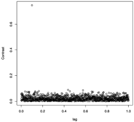
Figure 1: Fine grid case (FG). Over one simulation: displayed values of $|{\mathcal{U}}^{n}(\widetilde{\vartheta})|$ for $\widetilde{\vartheta}\in{\mathcal{G}}^{n}$ with mesh $h_{n}=10^{-3}$ and $\rho=0.75$. The value $\max_{\widetilde{\vartheta}\in{\mathcal{G}}^{n}}|{\mathcal{U}}^{n}(\widetilde{\vartheta})|$ is well located.

5.2 Synchronous data: Estimation results and their analysis

We repeat 300 simulations of the experiment and compute the value of $\widehat{\vartheta}_{n}$ each time, the true value being $\vartheta=0.1$, letting $\rho$ vary in $\{0.25,0.5,0.75\}$. We adopt the following terminology:

1. The fine grid estimation (abbreviated FG) with $h_{n}=10^{-3}$.

2. The moderate grid estimation (abbreviated MG) with $h_{n}=3.10^{-3}$.

3. The coarse grid estimation (abbreviated CG) with $h_{n}=6.10^{-3}$.

The estimation results are displayed in Table 1 below. With no surprise, for a given mesh $h_{n}$, the difficulty of the estimation problem increases as $\rho$ decreases.

In the fine grid approximation case (FG) with mesh $h_{n}=10^{-3}$, the lead-lag parameter $\vartheta$ belongs to ${\mathcal{G}}^{n}$ exactly. Therefore, the contrast ${\mathcal{U}}^{n}(\widehat{\vartheta})$ is close to $0$ for all values $\widetilde{\vartheta}\in{\mathcal{G}}^{n}$, except perhaps for the exact value $\widetilde{\vartheta}=\vartheta$. This is illustrated in Figure 1 and Figure 2 below, where we display the values or ${\mathcal{U}}^{n}(\widehat{\vartheta}_{n})$. Note how more scattered are the values of ${\mathcal{U}}^{n}(\widehat{\vartheta}_{n})$ for $\rho=0.25$ compared to $\rho=0.75$. This is, of course, no surprise.

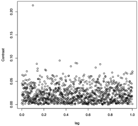
Figure 2: Same setting as in Figure 1 for $\rho=0.25$. The value $\max_{\widetilde{\vartheta}\in{\mathcal{G}}^{n}}|{\mathcal{U}}^{n}(\widetilde{\vartheta})|$ is still correctly located.

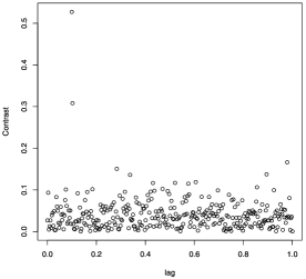
Figure 3: Moderate grid case (MG). Over one simulation: displayed values of $|{\mathcal{U}}^{n}(\widetilde{\vartheta})|$ for $\widetilde{\vartheta}\in{\mathcal{G}}^{n}$ with mesh $h_{n}=10^{-3}$ and $\rho=0.75$. The value $\max_{\widetilde{\vartheta}\in{\mathcal{G}}^{n}}|{\mathcal{U}}^{n}(\widetilde{\vartheta})|$ is still well located. We begin to see the effect of the maximization over a grid ${\mathcal{G}}^{n}$ which does not match exactly with the true value $\vartheta$ with the appearance of a second maximum.

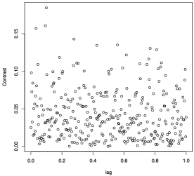
Figure 4: Same setting as in Figure 3 for $\rho=0.25$. The value $\max_{\widetilde{\vartheta}\in{\mathcal{G}}^{n}}|{\mathcal{U}}^{n}(\widetilde{\vartheta})|$ is still correctly located, but the overall shape of $|{\mathcal{U}}^{n}(\widetilde{\vartheta})|$ deteriorates.

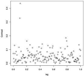
Figure 5: Coarse grid case (CG). Over one simulation: displayed values of $|{\mathcal{U}}^{n}(\widetilde{\vartheta})|$ for $\widetilde{\vartheta}\in{\mathcal{G}}^{n}$ with mesh $h_{n}=10^{-3}$ and $\rho=0.75$. The value $\max_{\widetilde{\vartheta}\in{\mathcal{G}}^{n}}|{\mathcal{U}}^{n}(\widetilde{\vartheta})|$ is still well located. The fact that ${\mathcal{G}}^{n}$ does not match $\vartheta$ appears more clearly than in Figure 3.

For the moderate grid (MG) and the coarse grid (CH) cases, the lead-lag parameter $\vartheta\notin{\mathcal{G}}^{n}.$ Hence, ${\mathcal{U}}^{n}(\widetilde{\vartheta})$ is close to $0$ for almost all values of ${\mathcal{G}}^{n}$ except but two. When $\rho$ is small, the statistical error in the estimation of $\rho$ is such that $|\max_{\widetilde{\vartheta}\in{\mathcal{G}}^{n}}{\mathcal{U}}^{n}(\widetilde{\vartheta})|$ is not well located anymore. The error in the estimation can then be substantial, but is nevertheless consistent with our convergence result. This is illustrated in Figures 3 to 8 below.

When $\rho$ decreases or when the mesh $h_{n}$ of the grid increases, the performance of $\widehat{\vartheta}_{n}$ deteriorates, as shown in Figures 7 and 8 below.

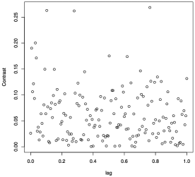
Figure 6: Same setting as in Figure 5 for $\rho=0.25$. The value $\max_{\widetilde{\vartheta}\in{\mathcal{G}}^{n}}|{\mathcal{U}}^{n}(\widetilde{\vartheta})|$ is no longer correctly located.

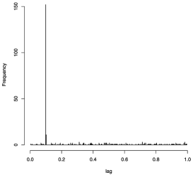
Figure 7: Moderate grid case (MG). Histogram of the values of $\widehat{\vartheta}_{n}$ with true value $\vartheta=0.1$ over $300$ simulations for $\rho=0.25$.

5.3 Non-synchronous data

We randomly pick 300 sampling times for $X$ over $[0,1]$ uniformly over a grid of mesh size $10^{-3}$. We randomly pick $300$ sampling times for $Y$ likewise, and independently of the sampling for $X$. The data generating process is the same as in Section 5.1. In Table 2, we display the estimation results for 300 simulations, in the fine gird case (FG) with $\vartheta=0.1$ and $\rho=0.75$.

The histograms for the case $\rho=0.5$ and $\rho=0.25$ are displayed in Figures 9 and 10.

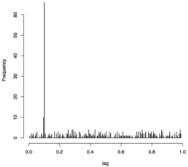
Figure 8: Coarse grid case (CG). Histogram of the values of $\widehat{\vartheta}_{n}$ with true value $\vartheta=0.1$ over $300$ simulations for $\rho=0.25$.

Table 2: Estimation of $\vartheta=0.1$ on 300 simulated samples for $\rho=0.75$ and non-synchronous data

$\widehat{\vartheta}$	0.099	0.1	0.101	0.102	0.103	0.104	0.105
FG, $\rho=0.75$	16	106	107	46	19	4	2

6 A numerical illustration on real data

Figure 9: Fine grid case (FG), non-synchronous data. Histogram of the values of $\widehat{\vartheta}_{n}$ with true value $\vartheta=0.1$ over $300$ simulations for $\rho=0.5$.

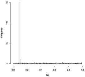
Figure 10: Fine grid case (FG), non-synchronous data. Histogram of the values of $\widehat{\vartheta}_{n}$ with true value $\vartheta=0.1$ over $300$ simulations for $\rho=0.25$. The performances of $\widehat{\vartheta}_{n}$ clearly deteriorates as compared to Figure 9.

6.1 The data set

We study here the lead-lag relationship between the following two financial assets:

• [-]

• The future contract on the DAX index (FDAX for short), with maturity December 2010.

• The Euro-Bund future contract (Bund for short), with maturity December 2010, which is an interest rate product based on a notional long-term debt instruments issued by the Federal Republic of Germany.

These two assets are electronically traded on the EUREX market, and are known to be highly liquid. Our data set has been provided by the company QuantHouse EUROPE/ASIA. It consists in all the trades for 20 days of October 2010. Each trading day starts at 8.00 am CET and finishes at 22.00 CET, and the accuracy in the timestamp values is one millisecond.

Figure 11: Signature plot for the Bund (left) and the FDAX (right) for 2010, October 13.

6.2 Methodology: A one day analysis

In order to explain our methodology, we take the example of a representative day: 2010, October 13.

Microstructure noise

Since high-frequency data are concerned, we need to incorporate microstructure noise effects, at least at an empirical level. A classical way to study the intensity of the microstructure noise is to draw the signature plot (here in trading time). The signature plot is a function from $\mathbb{N}$ to $\mathbb{R}^{+}$. To a given integer $k$, it associates the sum of the squared increments of the traded price (the realized volatility) when only 1 trade out of $k$ is considered for computing the traded price. If the price were coming from a continuous-time semi-martingale, the signature plot should be approximately flat. In practice, it is decreasing, as shown by Figure 11.

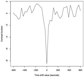
Figure 12: The function ${\mathcal{U}}^{n}$ for 2010, October 13, time shift values between $-10$ minutes and $10$ minutes, on a grid with mesh 30 seconds. The contrast is obtained by taking the absolute value of ${\mathcal{U}}^{n}$.

According to Figure 11, for all our considered day, we subsample our data so that we keep one trade out of 20. On 2010, October 13, after subsampling, it remains 2018 trades for the Bund and 3037 trades for the FDAX.

Construction of the contrast function

The second step is to compute our contrast function. Here the Bund plays the role of $X$ and the FDAX the role of $Y$. Therefore, if the estimated value is positive, it means that the Bund is the leader asset and the FDAX the lagger asset, and conversely. To have a first idea of the lead-lag value, we consider our contrast function for a time shift between $-10$ minutes and $10$ minutes, on a grid with mesh 30 seconds. The result of this computation for October 2010, 13 is given in Figure 12.

From Figure 12, we see that the lead-lag value is close to zero. Thus, we then compute the contrast function for a time shift between $-5$ seconds and $5$ seconds, on a grid with mesh 0.1 second. The result of this computation for 2010, October 13 is given in Figure 13.

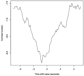
Figure 13: The function ${\mathcal{U}}^{n}$ for 2010, October 13, time shift values between $-5$ seconds and $5$ seconds, on a grid with mesh 0.1 second. The contrast is obtained by taking the absolute value of ${\mathcal{U}}^{n}$.

From Figure 13, we can conclude that on 2010, October 13, the FDAX seems to lead the Bund, with a small lead lag value of $-0.8$ second.

6.3 Systematic results over a one-month period

We now give, in Figure 14, the results for all the days of October 2010.

	Number of trades for the	Number of trades for the	Lead-lag
Day	bund (after subsampling)	FDAX (after subsampling)	(seconds)
1 October 2010	2847	4215	$-0.2$
5 October 2010	2213	3302	$-1.1$
6 October 2010	2244	2678	$-0.1$
7 October 2010	1897	3121	$-0.5$
8 October 2010	2545	2852	$-0.6$
11 October 2010	1050	1497	$-1.4$
12 October 2010	2265	3018	$-0.8$
13 October 2010	2018	3037	$-0.8$
14 October 2010	2057	2625	$-0.0$
15 October 2010	2571	3269	$-0.7$
18 October 2010	1727	2326	$-2.1$
19 October 2010	2527	3162	$-1.6$
20 October 2010	2328	2554	$-0.5$
21 October 2010	2263	3128	$-0.1$
22 October 2010	1894	1784	$-1.2$
25 October 2010	1501	2065	$-0.4$
26 October 2010	2049	2462	$-0.1$
27 October 2010	2606	2864	$-0.6$
28 October 2010	1980	2632	$-1.3$
29 October 2010	2262	2346	$-1.6$

Figure 14: Estimated lead-lag values for October 2010.

The results of Figure 14 seem to indicate that, on average, the FDAX tends to lead the Bund. Indeed, the estimated lead-lag values are systematically negative. Of course these results have to be taken with care since the estimated values are relatively small (the order of one second); however, dealing with highly traded assets on electronic markets, the order of magnitude of the lead-lag values that we find are no surprise and are consistent with common knowledge. A possible interpretation – yet speculative at the exploratory level intended here – for the presence of such lead-lag effects is the difference between the tick sizes of the different assets. Indeed, the negative values could mean that the tick size of the FDAX can be considered smaller than those of the Bund.

Appendix

.1 Proof of Proposition 1

For notational clarity, for a given interval $I=(\underline{I},\overline{I}]$, we may sometimes write $X(\underline{I},\overline{I})$ instead of $X(I)$ when no confusion is possible. In the Bachelier case with lead-lag parameter $\vartheta\in\Theta$, we work with the following explicit representation of the observation process:

$$\cases{X_{t}=x_{0}+\sigma_{1}B_{t},\vspace*{2pt}\cr Y_{t}=y_{0}+\sigma_{2}\bigl{(}\rho B_{t-\vartheta}+\sqrt{1-\rho^{2}}W_{t-\vartheta}\bigr{)},}$$ (13)

where $B$ and $W$ are two independent Brownian motions. We have

$${\mathcal{U}}^{n}(\tilde{\vartheta})=\sum_{0\leq i\Delta_{n}\leq T}X\bigl{(}(i-1)\Delta_{n},i\Delta_{n}\bigr{)}\tau_{-\tilde{\vartheta}}Y\bigl{(}(i-1)\Delta_{n},i\Delta_{n}\bigr{)}=\sigma_{1}\sigma_{2}\sum_{0\leq i\Delta_{n}\leq T}\chi_{i}^{n}(\tilde{\vartheta}),$$

with

$$\chi_{i}^{n}(\tilde{\vartheta})=B\bigl{(}(i-1)\Delta_{n},i\Delta_{n}\bigr{)}\bigl{[}\rho\tau_{\vartheta-\tilde{\vartheta}}B\bigl{(}(i-1)\Delta_{n},i\Delta_{n}\bigr{)}+\sqrt{1-\rho^{2}}\tau_{\vartheta-\tilde{\vartheta}}W\bigl{(}(i-1)\Delta_{n},i\Delta_{n}\bigr{)}\bigr{]}.$$

We have

$$\mathbb{E}[\chi_{i}^{n}(\tilde{\vartheta})]=\rho\mathbb{E}\bigl{[}B\bigl{(}(i-1)\Delta_{n},i\Delta_{n}\bigr{)}\tau_{\vartheta-\tilde{\vartheta}}B\bigl{(}(i-1)\Delta_{n},i\Delta_{n}\bigr{)}\bigr{]}=\rho\Delta_{n}\varphi\bigl{(}\Delta_{n}^{-1}(\tilde{\vartheta}-\vartheta)\bigr{)},$$

where $\varphi(x)=(1-|x|)1_{|x|\leq 1}$ is the usual hat function. Assuming further, with no loss of generality, that $T/\Delta_{n}$ is an integer, we obtain the representation

$${\mathcal{U}}^{n}(\tilde{\vartheta})=\sigma_{1}\sigma_{2}T\biggl{(}\rho\varphi\bigl{(}\Delta_{n}^{-1}(\vartheta-\tilde{\vartheta})\bigr{)}+T^{-1}\sum_{0\leq i\Delta_{n}\leq T}\bigl{(}\chi_{i}^{n}(\tilde{\vartheta})-\mathbb{E}[\chi_{i}^{n}(\tilde{\vartheta})]\bigr{)}\biggr{)}.$$

We now assume without loss of generality that $0\leq\vartheta-\tilde{\vartheta}\leq\Delta_{n}$ (the symmetric case being treated the same way). The sequence of random variables $\chi_{i}^{n}(\tilde{\vartheta})$ is stationary. Moreover, since the random variable $\chi_{i}^{n}(\tilde{\vartheta})$ involves increments of $W$ and $B$ over a domain included in $[(i-2)\Delta_{n},i\Delta_{n}]$ because $|\vartheta-\tilde{\vartheta}|\leq\Delta_{n}$, it follows that $\chi_{i}^{n}(\tilde{\vartheta})$ and $\chi_{j}^{n}(\tilde{\vartheta})$ are independent as soon as $|i-j|\geq 2$. Moreover, we claim that

$$\operatorname{Cov}(\chi_{i}^{n}(\tilde{\vartheta}),\chi_{j}^{n}(\tilde{\vartheta}))=0\qquad\mbox{if }|i-j|=1.$$ (14)

Therefore, by the central limit theorem, we have that

$$\Delta_{n}^{1/2}T^{-1/2}\sum_{0\leq i\Delta_{n}\leq T}\bigl{(}\chi_{i}^{n}(\tilde{\vartheta})-\mathbb{E}[\chi_{i}^{n}(\tilde{\vartheta})]\bigr{)}$$

is approximately centred Gaussian, with variance

$$\operatorname{Var}(\chi_{1}^{n}(\tilde{\vartheta})).$$

Computation of $\operatorname{Var}(\chi_{1}^{n}(\tilde{\vartheta}))$

To that end, we need to evaluate

$$\mathrm{I}=\rho^{2}\mathbb{E}[(B(0,\Delta_{n})\tau_{\vartheta-\tilde{\vartheta}}B(0,\Delta_{n}))^{2}],$$

and

$$\mathrm{II}=(1-\rho^{2})\mathbb{E}[(B(0,\Delta_{n})\tau_{\vartheta-\tilde{\vartheta}}W(0,\Delta_{n}))^{2}],$$

since $B(0,\Delta_{n})\tau_{\vartheta-\tilde{\vartheta}}B(0,\Delta_{n})$ and $B(0,\Delta_{n})\tau_{\vartheta-\tilde{\vartheta}}W(0,\Delta_{n})$ are uncorrelated. Writing

$$B(0,\Delta_{n})\tau_{\vartheta-\tilde{\vartheta}}B(0,\Delta_{n})$$

$$\quad=\bigl{(}B(0,\vartheta-\tilde{\vartheta})+B(\vartheta-\tilde{\vartheta},\Delta_{n})\bigr{)}\bigl{(}B(\vartheta-\tilde{\vartheta},\Delta_{n})+B(\Delta_{n},\vartheta-\tilde{\vartheta}+\Delta_{n})\bigr{)},$$

taking square and expectation, we readily obtain that

$$\mathrm{I} = 2\rho^{2}(\vartheta-\tilde{\vartheta})\bigl{(}\Delta_{n}-(\vartheta-\tilde{\vartheta})\bigr{)}+\rho^{2}(\vartheta-\tilde{\vartheta})^{2}+3\rho^{2}\bigl{(}\Delta_{n}-(\vartheta-\tilde{\vartheta})\bigr{)}^{2}$$

$$= \rho^{2}\bigl{(}\Delta_{n}^{2}\bigl{(}1+2\varphi\bigl{(}\Delta_{n}^{-1}(\vartheta-\tilde{\vartheta})\bigr{)}^{2}\bigr{)}\bigr{)}.$$

Concerning II, since $B$ and $W$ are independent, we readily have

$$\mathrm{II}=(1-\rho^{2})\Delta_{n}^{2},$$

therefore, from $\mathbb{E}[\chi_{1}^{n}(\tilde{\vartheta})]=\rho\Delta_{n}\varphi(\Delta_{n}^{-1}(\tilde{\vartheta}-\vartheta))$, we finally infer

$$\Delta_{n}^{-2}\operatorname{Var}(\chi_{1}^{n}(\tilde{\vartheta}))=1+\rho^{2}\varphi\bigl{(}\Delta_{n}^{-1}(\vartheta-\tilde{\vartheta})\bigr{)}^{2}$$

from which Proposition 1 follows. It remains to prove (14). By stationarity, this amounts to evaluate

$$\rho^{2}\mathbb{E}[B(0,\Delta_{n})B(\vartheta-\tilde{\vartheta},\Delta_{n}+\vartheta-\tilde{\vartheta})B(\Delta_{n},2\Delta_{n})B(\Delta_{n}+\vartheta-\tilde{\vartheta},2\Delta_{n}+\vartheta-\tilde{\vartheta})]-\mathbb{E}[\chi_{1}^{n}(\vartheta)]^{2}.$$

To that end, we split each of the terms as follows:

$$B(0,\Delta_{n}) = B(0,\vartheta-\tilde{\vartheta})+B(\vartheta-\tilde{\vartheta},\Delta_{n}),$$

$$B(\vartheta-\tilde{\vartheta},\Delta_{n}+\vartheta-\tilde{\vartheta}) = B(\vartheta-\tilde{\vartheta},\Delta_{n})+B(\Delta_{n}+\vartheta-\tilde{\vartheta}),$$

$$B(\Delta_{n},2\Delta_{n}) = B(\Delta_{n},\Delta_{n}+\vartheta-\tilde{\vartheta})+B(\Delta_{n}+\vartheta-\tilde{\vartheta},2\Delta_{n}),$$

$$B(\Delta_{n}+\vartheta-\tilde{\vartheta},2\Delta_{n}+\vartheta-\tilde{\vartheta}) = B(\Delta_{n}+\vartheta-\tilde{\vartheta},2\Delta_{n})+B(2\Delta_{n},2\Delta_{n}+\vartheta-\tilde{\vartheta}).$$

Using the stochastic independence of each of these terms, multiplying and integrating, we easily obtain

$$\rho^{2}\mathbb{E}[B(0,\Delta_{n})B(\vartheta-\tilde{\vartheta},\Delta_{n}+\vartheta-\tilde{\vartheta})B(\Delta_{n},2\Delta_{n})B(\Delta_{n}+\vartheta-\tilde{\vartheta},2\Delta_{n}+\vartheta-\tilde{\vartheta})]$$

$$\quad=\rho^{2}\Delta_{n}^{2}\varphi\bigl{(}\Delta_{n}^{-1}(\vartheta-\tilde{\vartheta})\bigr{)}^{2}=\mathbb{E}[\chi_{1}^{n}(\tilde{\vartheta})]^{2}.$$

.2 Proof of Proposition 2

Suppose that $\Delta_{n}^{-1}(\widehat{\vartheta}_{n}-\vartheta)\rightarrow Z$, in law, for some random random variable $Z$. For $a\in\mathbb{R}$, we write $a^{[n]},$ the best approximation of $a$ by a point of the form $k\Delta_{n}$, $k\in\mathbb{Z}$ and $a^{\lfloor n\rfloor}$, the best approximation of $a$ by a point smaller or equal to $a$ and of the form $k\Delta_{n}$, $k\in\mathbb{Z}$. We have

$$\Delta_{n}^{-1}(\widehat{\vartheta}_{n}-\vartheta)=\Delta_{n}^{-1}\bigl{(}\widehat{\vartheta}_{n}-\widehat{\vartheta}_{n}^{\lfloor n\rfloor}\bigr{)}+\Delta_{n}^{-1}\bigl{(}\widehat{\vartheta}_{n}^{\lfloor n\rfloor}-\vartheta\bigr{)}.$$

The first term in the right-hand side of the equality is smaller than $\Delta_{n}^{-1}h_{n}$ and so converges to zero. The second term can be written as

$$\Delta_{n}^{-1}\bigl{(}\widehat{\vartheta}_{n}^{\lfloor n\rfloor}-\vartheta^{[n]}\bigr{)}+\Delta_{n}^{-1}\bigl{(}\vartheta^{[n]}-\vartheta\bigr{)}=T_{1,n}+T_{2,n},$$

say. The sequence $T_{1,n}$ is a random sequence of integers, and $T_{2,n}$ is a deterministic sequence with values in $[0,1/2]$ which does not converge. Let $\psi_{n}$ be a subsequence such that $T_{2,\psi_{n}}\rightarrow l$ with $l\in(0,1/2]$. Then $T_{1,\psi_{n}}$ converges in law to $Z-l$ which implies that the support of $Z$ is included in $\{z+l,z\in\mathbb{Z}\}$. Consider now $\widetilde{\psi}_{n}$ such that $T_{2,\widetilde{\psi}_{n}}\rightarrow l^{\prime}$ with $l^{\prime}\in[0,1/2]$, $l^{\prime}\neq l$. In the same way, we get that the support of $Z$ is also included in $\{z+l^{\prime},z\in\mathbb{Z}\}$, a contradiction.

.3 Proof of Lemma 1

Preliminary results

We first prove the following results.

Lemma 3.

Work under Assumption B2, under the slightly more general assumption that for all $I=[\underline{I,\overline{I}})\in{\mathcal{I}}$, the random variables $\underline{I}$ and $\overline{I}$ are $\mathbb{F}$-stopping times.

1. [(a)]

2. If $\widetilde{\vartheta}\geq\vartheta+v_{n}$, then for any $\mathbb{F}$-stopping time $\sigma$ and $t\in\mathbb{R}_{+}$, $\sigma+\widetilde{\vartheta}$ is an $\mathbb{F}^{\vartheta+v_{n}}$-stopping time. In particular, the random variables $\underline{I^{n}_{\widetilde{\vartheta}}}$ and $\overline{I^{n}_{\widetilde{\vartheta}}}$ are $\mathbb{F}^{\vartheta+v_{n}}$-stopping times.

3. For each $J\in{\mathcal{J}}$, we have

   $$\mathcal{F}^{\vartheta+v_{n}}_{\overline{J^{n}}}\subset\mathcal{F}^{\vartheta+v_{n}}_{\underline{J^{n}}+v_{n}}=\mathcal{F}^{\vartheta}_{\underline{J^{n}}},$$

   and for each $I\in{\mathcal{I}}$,

   $$\mathcal{F}_{\overline{I^{n}}}=\mathcal{F}^{\vartheta+v_{n}}_{\overline{I^{n}_{(\vartheta+v_{n})}}}.$$

4. Suppose that $\widetilde{\vartheta}\geq\vartheta+\varepsilon_{n}$ and $2v_{n}\leq\varepsilon_{n}$. Then for any random variable $X^{\prime}$ measurable w.r.t. $\mathcal{F}_{\overline{I^{n}}}$, the random variables $X^{\prime}1_{\{\underline{I^{n}_{\widetilde{\vartheta}}}\leq\overline{J^{n}}\}}$ and $X^{\prime}1_{\{\underline{I^{n}_{\widetilde{\vartheta}}}<\overline{J^{n}}\}}$ are $\mathcal{F}^{\vartheta}_{\underline{J^{n}}}$-measurable.

Proof.

Proof of (a). For any $\mathbb{F}$-stopping time $\sigma$ and $t\in\mathbb{R}_{+}$,

$$\{\sigma+\widetilde{\vartheta}\leq t\} = \{\sigma\leq t-\widetilde{\vartheta}\}=\bigl{\{}\sigma\leq\bigl{(}t-(\widetilde{\vartheta}-\vartheta-v_{n})\bigr{)}-\vartheta-v_{n}\bigr{\}}$$

$$\in \mathcal{F}^{\vartheta+v_{n}}_{t-(\widetilde{\vartheta}-\vartheta-v_{n})}\subset\mathcal{F}^{\vartheta+v_{n}}_{t}.$$

Proof of (b). Note first that under Assumption B2, the $\mathbb{F}^{\vartheta+v_{n}}$-stopping time $\underline{J^{n}}$ is in particular an $\mathbb{F}^{\vartheta}$-stopping time; thus $\mathcal{F}^{\vartheta}_{\underline{J^{n}}}$ is a $\sigma$-field. Moreover, since $\overline{J^{n}}$ and $\underline{J^{n}}+v_{n}$ are $\mathbb{F}^{\vartheta+v_{n}}$-stopping times by definition, both $\mathcal{F}^{\vartheta+v_{n}}_{\overline{J^{n}}}$ and $\mathcal{F}^{\vartheta+v_{n}}_{\underline{J^{n}}+v_{n}}$ are $\sigma$-fields, and also the inclusion is trivial from $\overline{J^{n}}\leq\underline{J^{n}}+v_{n}$. To obtain the equality, it suffices to observe that each of the conditions “${\mathcal{A}}\in\mathcal{F}^{\vartheta+v_{n}}_{\underline{J^{n}}+v_{n}}$” and “${\mathcal{A}}\in\mathcal{F}^{\vartheta}_{\underline{J^{n}}}$” is equivalent to the condition

$${\mathcal{A}}\cap\{\underline{J^{n}}\leq t-v_{n}\}\in\mathcal{F}^{\vartheta}_{t-v_{n}}$$

for all $t\in\mathbb{R}_{+}$. The second equality is proved in the same way.

Proof of (c). Since $\overline{J^{n}}$ and $\underline{I^{n}_{\widetilde{\vartheta}}}$ are $\mathbb{F}^{\vartheta+v_{n}}$-stopping times by assumption, we have

$$\{\underline{I^{n}_{\widetilde{\vartheta}}}\leq\overline{J^{n}}\}\in\mathcal{F}^{\vartheta+v_{n}}_{\overline{J^{n}}}\subset\mathcal{F}^{\vartheta}_{\underline{J^{n}}},$$

the last inclusion following from (b). If $\underline{I^{n}_{\widetilde{\vartheta}}}\leq\overline{J^{n}}$, then

$$\overline{I^{n}}\leq\underline{I^{n}}+v_{n}\leq\overline{J^{n}}-\widetilde{\vartheta}+v_{n}\leq\overline{J^{n}}-\vartheta-v_{n},$$

which implies $\overline{I^{n}_{\vartheta+v_{n}}}\leq\overline{J^{n}}.$ Thus

$$X^{\prime}1_{\{\underline{I^{n}_{\widetilde{\vartheta}}}\leq\overline{J^{n}}\}}=X^{\prime}1_{\{\overline{I^{n}_{(\vartheta+v_{n})}}\leq\overline{J^{n}}\}}\times 1_{\{\underline{I^{n}_{\widetilde{\vartheta}}}\leq\overline{J^{n}}\}}.$$

We have that $X^{\prime}$ is measurable with respect to $\mathcal{F}_{\overline{I^{n}}}=\mathcal{F}^{\vartheta+v_{n}}_{\overline{I^{n}_{(\vartheta+v_{n})}}}$. Also $\overline{I^{n}_{(\vartheta+v_{n})}}$ is a stopping time with respect to $\mathbb{F}^{\vartheta+v_{n}}$ by (a). Consequently, $X^{\prime}1_{\{\overline{I^{n}_{(\vartheta+v_{n})}}\leq\overline{J^{n}}\}}$ is $\mathcal{F}^{\vartheta+v_{n}}_{\overline{J^{n}}}$-measurable, hence $\mathcal{F}^{\vartheta}_{\underline{J^{n}}}$-measurable. Eventually, $X^{\prime}1_{\{\underline{I^{n}_{\widetilde{\vartheta}}}\leq\overline{J^{n}}\}}$ is $\mathcal{F}^{\vartheta}_{\underline{J^{n}}}$-measurable. The other statement is proved the same way. ∎

Proof of Lemma 1 We have

$$X^{\prime}K(I^{n}_{\widetilde{\vartheta}},J^{n})=X^{\prime}1_{\{\underline{I^{n}_{\widetilde{\vartheta}}}\leq\underline{J^{n}}\}}1_{\{\underline{J^{n}}<\overline{I^{n}_{\widetilde{\vartheta}}}\}}+X^{\prime}1_{\{\underline{I^{n}_{\widetilde{\vartheta}}}>\underline{J^{n}}\}}1_{\{\overline{J^{n}}>\underline{I^{n}_{\widetilde{\vartheta}}}\}}.$$

Since $\widetilde{\vartheta}\geq\vartheta+\varepsilon_{n}\geq\vartheta+v_{n}$, both $\underline{I^{n}_{\widetilde{\vartheta}}}$ and $\overline{I^{n}_{\widetilde{\vartheta}}}$ are $\mathbb{F}^{\vartheta+v_{n}}$-stopping times. Therefore, the second term on the right-hand side of the above equality is $\mathcal{F}^{\vartheta}_{\underline{J^{n}}}$-measurable by (c) of Lemma 3.

Now we notice that if $\underline{I^{n}_{\widetilde{\vartheta}}}\leq\underline{J^{n}}$, then $\underline{I^{n}_{\widetilde{\vartheta}}}\leq\overline{J^{n}}$, therefore

$$X^{\prime}1_{\{\underline{I^{n}_{\widetilde{\vartheta}}}\leq\underline{J^{n}}\}}1_{\{\underline{J^{n}}<\overline{I^{n}_{\widetilde{\vartheta}}}\}}=\bigl{(}X^{\prime}1_{\{\underline{I^{n}_{\widetilde{\vartheta}}}\leq\overline{J^{n}}\}}\bigr{)}\times\bigl{(}1_{\{\underline{I^{n}_{\widetilde{\vartheta}}}\leq\underline{J^{n}}\}}1_{\{\underline{J^{n}}<\overline{I^{n}_{\widetilde{\vartheta}}}\}}\bigr{)}.$$

The first factor on the right-hand side of the above equality is $\mathcal{F}^{\vartheta}_{\underline{J^{n}}}$-measurable by (c) of Lemma 3, and the second factor is obviously $\mathcal{F}^{\vartheta}_{\underline{J^{n}}}$-measurable. This completes the proof.

.4 Proof of Lemma 2

Let us fix $I\in{\mathcal{I}}$. Let

$$T_{J}=\cases{\overline{I^{n}}-v_{n}&\quad$\mbox{on }\{\overline{\widetilde{J}^{n}_{-\delta_{n}}}>\overline{I^{n}}\}$,\vspace*{2pt}\cr\overline{\widetilde{J}^{n}}_{-\delta_{n}}&\quad$\mbox{on }\{\overline{\widetilde{J}^{n}_{-\delta_{n}}}\leq\overline{I^{n}}\}.$}$$

We know that $\overline{I^{n}}-v_{n}$ is an $\mathbb{F}$-stopping time by Assumption B2, and also that $\overline{\widetilde{J}^{n}_{-\delta_{n}}}-v_{n}$ is an $\mathbb{F}$-stopping time due to $\delta_{n}\leq 0$. Let us show first that the $T_{J}$s are $\mathbb{F}$-stopping times. Let $t\in[-\delta,T+\delta]$. Let

$${\mathcal{A}}_{1}=\{\overline{I^{n}}-v_{n}\leq t,\overline{\widetilde{J}^{n}_{-\delta_{n}}}-v_{n}>\overline{I^{n}}-v_{n}\}$$

and

$${\mathcal{A}}_{2}=\{\overline{\widetilde{J}^{n}}_{-\delta_{n}}\leq t,\overline{\widetilde{J}^{n}_{-\delta_{n}}}-v_{n}\leq\overline{I^{n}}-v_{n}\}.$$

It is obvious that ${\mathcal{A}}_{1}\in\mathcal{F}_{t}$ since $\overline{I^{n}}-v_{n}$ is an $\mathbb{F}$-stopping time and also

$$\{\overline{\widetilde{J}^{n}_{-\delta_{n}}}-v_{n}\geq\overline{I^{n}}-v_{n}\}\in\mathcal{F}_{\overline{I^{n}}-v_{n}}.$$

For the term ${\mathcal{A}}_{2}$, if $t\in[-\delta,-\delta+v_{n}]$, then ${\mathcal{A}}_{2}=\varnothing\in\mathcal{F}_{-\delta}\subset\mathcal{F}_{t}$. Otherwise, if $t\in(-\delta+v_{n},T+\delta]$, then

$${\mathcal{A}}_{2}=\{\overline{\widetilde{J}^{n}_{-\delta_{n}}}-v_{n}\leq t-v_{n},\overline{\widetilde{J}^{n}_{-\delta_{n}}}-v_{n}\leq\overline{I^{n}}-v_{n}\}\in\mathcal{F}_{t-v_{n}}\subset\mathcal{F}_{t}.$$

Eventually, we have $\{T_{J}\leq t\}\in\mathcal{F}_{t}$; hence $T_{J}$ is an $\mathbb{F}$-stopping time.

In conclusion, there exists at least one $\overline{\widetilde{J}^{n}_{-\delta_{n}}}$ in $[\overline{I^{n}}-v_{n},\overline{I^{n}}]$. Therefore, we have $M^{I}=\sup_{J}T_{J}$, and this implies that $M^{I}$ is also an $\mathbb{F}$-stopping time.

References

- [1] {barticle}[mr] \bauthor\bsnmBandi, \bfnmF. M.\binitsF.M. &\bauthor\bsnmRussell, \bfnmJ. R.\binitsJ.R. (\byear2008). \btitleMicrostructure noise, realized variance, and optimal sampling. \bjournalRev. Econom. Stud. \bvolume75 \bpages339–369. \biddoi=10.1111/j.1467-937X.2008.00474.x, issn=0034-6527, mr=2398721 \bptokimsref \endbibitem
- [2] {barticle}[mr] \bauthor\bsnmBarndorff-Nielsen, \bfnmOle E.\binitsO.E., \bauthor\bsnmHansen, \bfnmPeter Reinhard\binitsP.R., \bauthor\bsnmLunde, \bfnmAsger\binitsA. &\bauthor\bsnmShephard, \bfnmNeil\binitsN. (\byear2008). \btitleDesigning realized kernels to measure the ex post variation of equity prices in the presence of noise. \bjournalEconometrica \bvolume76 \bpages1481–1536. \biddoi=10.3982/ECTA6495, issn=0012-9682, mr=2468558 \bptokimsref \endbibitem
- [3] {barticle}[auto:STB—2011/12/30—12:36:46] \bauthor\bsnmChiao, \bfnmC.\binitsC., \bauthor\bsnmHung, \bfnmK.\binitsK. &\bauthor\bsnmLee, \bfnmC. F.\binitsC.F. (\byear2004). \btitleThe price adjustment and lead-lag relations between stock returns: Microstructure evidence from the Taiwan stock market. \bjournalEmpirical Finance \bvolume11 \bpages709–731. \bptokimsref \endbibitem
- [4] {barticle}[auto:STB—2011/12/30—12:36:46] \bauthor\bsnmComte, \bfnmF.\binitsF. &\bauthor\bsnmRenaut, \bfnmE.\binitsE. (\byear1996). \btitleNon-causality in continuous time models. \bjournalEconometric Theory \bvolume12 \bpages215–256. \bptokimsref \endbibitem
- [5] {bmisc}[auto:STB—2011/12/30—12:36:46] \bauthor\bsnmDalalyan, \bfnmA.\binitsA. &\bauthor\bsnmYoshida, \bfnmN.\binitsN. (\byear2008). \bhowpublishedSecond-order asymptotic expansion for the covariance estimator of two asynchronously observed diffusion processes. Preprint. Available at arXiv:0804.0676. \bptokimsref \endbibitem
- [6] {barticle}[auto:STB—2011/12/30—12:36:46] \bauthor\bparticlede \bsnmJong, \bfnmF.\binitsF. &\bauthor\bsnmNijman, \bfnmT.\binitsT. (\byear1997). \btitleHigh frequency analysis of Lead-Lag relationships between financial markets. \bjournalJournal of Empirical Finance \bvolume4 \bpages259–277. \bptokimsref \endbibitem
- [7] {barticle}[mr] \bauthor\bsnmGenon-Catalot, \bfnmValentine\binitsV. &\bauthor\bsnmJacod, \bfnmJean\binitsJ. (\byear1993). \btitleOn the estimation of the diffusion coefficient for multi-dimensional diffusion processes. \bjournalAnn. Inst. Henri Poincaré Probab. Stat. \bvolume29 \bpages119–151. \bidissn=0246-0203, mr=1204521 \bptokimsref \endbibitem
- [8] {barticle}[mr] \bauthor\bsnmHansen, \bfnmPeter R.\binitsP.R. &\bauthor\bsnmLunde, \bfnmAsger\binitsA. (\byear2006). \btitleRealized variance and market microstructure noise. \bjournalJ. Bus. Econom. Statist. \bvolume24 \bpages127–161. \biddoi=10.1198/073500106000000071, issn=0735-0015, mr=2234447 \bptnotecheck related \bptokimsref \endbibitem
- [9] {barticle}[mr] \bauthor\bsnmHayashi, \bfnmTakaki\binitsT. &\bauthor\bsnmKusuoka, \bfnmShigeo\binitsS. (\byear2008). \btitleConsistent estimation of covariation under nonsynchronicity. \bjournalStat. Inference Stoch. Process. \bvolume11 \bpages93–106. \biddoi=10.1007/s11203-007-9009-9, issn=1387-0874, mr=2357555 \bptokimsref \endbibitem
- [10] {bmisc}[auto:STB—2011/12/30—12:36:46] \bauthor\bsnmHayashi, \bfnmT.\binitsT. &\bauthor\bsnmYoshida, \bfnmN.\binitsN. (\byear2005). \bhowpublishedEstimating correlations with missing observations in continuous diffusion models. Preprint. \bptokimsref \endbibitem
- [11] {barticle}[mr] \bauthor\bsnmHayashi, \bfnmTakaki\binitsT. &\bauthor\bsnmYoshida, \bfnmNakahiro\binitsN. (\byear2005). \btitleOn covariance estimation of non-synchronously observed diffusion processes. \bjournalBernoulli \bvolume11 \bpages359–379. \biddoi=10.3150/bj/1116340299, issn=1350-7265, mr=2132731 \bptokimsref \endbibitem
- [12] {bmisc}[auto:STB—2011/12/30—12:36:46] \bauthor\bsnmHayashi, \bfnmT.\binitsT. &\bauthor\bsnmYoshida, \bfnmN.\binitsN. (\byear2006). \bhowpublishedNonsynchronous covariance estimator and limit theorem. Research Memorandum 1020, Institute of Statistical Mathematics. \bptokimsref \endbibitem
- [13] {barticle}[mr] \bauthor\bsnmHayashi, \bfnmTakaki\binitsT. &\bauthor\bsnmYoshida, \bfnmNakahiro\binitsN. (\byear2008). \btitleAsymptotic normality of a covariance estimator for nonsynchronously observed diffusion processes. \bjournalAnn. Inst. Statist. Math. \bvolume60 \bpages367–406. \biddoi=10.1007/s10463-007-0138-0, issn=0020-3157, mr=2403524 \bptokimsref \endbibitem
- [14] {bmisc}[auto:STB—2011/12/30—12:36:46] \bauthor\bsnmHayashi, \bfnmT.\binitsT. &\bauthor\bsnmYoshida, \bfnmN.\binitsN. (\byear2008). \bhowpublishedNonsynchronous covariance estimator and limit theorem II. Research Memorandum 1067, Institute of Statistical Mathematics. \bptokimsref \endbibitem
- [15] {barticle}[mr] \bauthor\bsnmHoshikawa, \bfnmToshiya\binitsT., \bauthor\bsnmNagai, \bfnmKeiji\binitsK., \bauthor\bsnmKanatani, \bfnmTaro\binitsT. &\bauthor\bsnmNishiyama, \bfnmYoshihiko\binitsY. (\byear2008). \btitleNonparametric estimation methods of integrated multivariate volatilities. \bjournalEconometric Rev. \bvolume27 \bpages112–138. \biddoi=10.1080/07474930701853855, issn=0747-4938, mr=2424809 \bptokimsref \endbibitem
- [16] {bbook}[mr] \bauthor\bsnmIbragimov, \bfnmI. A.\binitsI.A. &\bauthor\bsnmHasminskiĭ, \bfnmR. Z.\binitsR.Z. (\byear1981). \btitleStatistical Estimation, Asymptotic Theory. \bseriesApplications of Mathematics \bvolume16. \baddressNew York: \bpublisherSpringer. \bnoteTranslated from the Russian by Samuel Kotz. \bidmr=0620321 \bptokimsref \endbibitem
- [17] {barticle}[mr] \bauthor\bsnmJacod, \bfnmJean\binitsJ., \bauthor\bsnmLi, \bfnmYingying\binitsY., \bauthor\bsnmMykland, \bfnmPer A.\binitsP.A., \bauthor\bsnmPodolskij, \bfnmMark\binitsM. &\bauthor\bsnmVetter, \bfnmMathias\binitsM. (\byear2009). \btitleMicrostructure noise in the continuous case: The pre-averaging approach. \bjournalStochastic Process. Appl. \bvolume119 \bpages2249–2276. \biddoi=10.1016/j.spa.2008.11.004, issn=0304-4149, mr=2531091 \bptokimsref \endbibitem
- [18] {barticle}[auto:STB—2011/12/30—12:36:46] \bauthor\bsnmKang, \bfnmJ.\binitsJ., \bauthor\bsnmLee, \bfnmC.\binitsC. &\bauthor\bsnmLee, \bfnmS.\binitsS. (\byear2006). \btitleEmpirical investigation of the lead-lag relations of returns and volatilities among the KOSPI200 spot, futures and options markets and their explanations. \bjournalJournal of Emerging Market Finance \bvolume5 \bpages235–261. \bptokimsref \endbibitem
- [19] {barticle}[mr] \bauthor\bsnmMalliavin, \bfnmPaul\binitsP. &\bauthor\bsnmMancino, \bfnmMaria Elvira\binitsM.E. (\byear2002). \btitleFourier series method for measurement of multivariate volatilities. \bjournalFinance Stoch. \bvolume6 \bpages49–61. \biddoi=10.1007/s780-002-8400-6, issn=0949-2984, mr=1885583 \bptokimsref \endbibitem
- [20] {bmisc}[auto:STB—2011/12/30—12:36:46] \bauthor\bsnmO’Connor, \bfnmM.\binitsM. (\byear1999). \bhowpublishedThe cross-sectional relationship between trading costs and lead/lag effects in stock & option markets. The Financial Review 34 95–117. \bptokimsref \endbibitem
- [21] {bmisc}[auto:STB—2011/12/30—12:36:46] \bauthor\bsnmRobert, \bfnmC. Y.\binitsC.Y. &\bauthor\bsnmRosenbaum, \bfnmM.\binitsM. (\byear2011). \bhowpublishedA new approach for the dynamics of ultra high frequency data: The model with uncertainty zones. Journal of Financial Econometrics 9 344–366. \bptokimsref \endbibitem
- [22] {bmisc}[auto:STB—2011/12/30—12:36:46] \bauthor\bsnmRobert, \bfnmC. Y.\binitsC.Y. &\bauthor\bsnmRosenbaum, \bfnmM.\binitsM. (\byear2012). \bhowpublishedVolatility and covariation estimation when microstructure noise and trading times are endogenous. Math. Finance 22 133–164. \bptokimsref \endbibitem
- [23] {barticle}[mr] \bauthor\bsnmRobert, \bfnmChristian Y.\binitsC.Y. &\bauthor\bsnmRosenbaum, \bfnmMathieu\binitsM. (\byear2010). \btitleOn the limiting spectral distribution of the covariance matrices of time-lagged processes. \bjournalJ. Multivariate Anal. \bvolume101 \bpages2434–2451. \biddoi=10.1016/j.jmva.2010.06.014, issn=0047-259X, mr=2719873 \bptokimsref \endbibitem
- [24] {barticle}[mr] \bauthor\bsnmRosenbaum, \bfnmMathieu\binitsM. (\byear2009). \btitleIntegrated volatility and round-off error. \bjournalBernoulli \bvolume15 \bpages687–720. \biddoi=10.3150/08-BEJ170, issn=1350-7265, mr=2555195 \bptokimsref \endbibitem
- [25] {barticle}[mr] \bauthor\bsnmRosenbaum, \bfnmMathieu\binitsM. (\byear2011). \btitleA new microstructure noise index. \bjournalQuant. Finance \bvolume11 \bpages883–899. \biddoi=10.1080/14697680903514352, issn=1469-7688, mr=2806970\bptnotecheck year \bptokimsref \endbibitem
- [26] {bmisc}[auto:STB—2011/12/30—12:36:46] \bauthor\bsnmUbukata, \bfnmM.\binitsM. &\bauthor\bsnmOya, \bfnmK.\binitsK. (\byear2008). \bhowpublishedA test for dependence and covariance estimator of market microstructure noise. Discussion Papers in Economics And Business, 07-03-Rev.2, 112–138. \bptokimsref \endbibitem
- [27] {barticle}[mr] \bauthor\bsnmZhang, \bfnmLan\binitsL. (\byear2011). \btitleEstimating covariation: Epps effect, microstructure noise. \bjournalJ. Econometrics \bvolume160 \bpages33–47. \biddoi=10.1016/j.jeconom.2010.03.012, issn=0304-4076, mr=2745865 \bptnotecheck year \bptokimsref \endbibitem
- [28] {barticle}[mr] \bauthor\bsnmZhang, \bfnmLan\binitsL., \bauthor\bsnmMykland, \bfnmPer A.\binitsP.A. &\bauthor\bsnmAït-Sahalia, \bfnmYacine\binitsY. (\byear2005). \btitleA tale of two time scales: Determining integrated volatility with noisy high-frequency data. \bjournalJ. Amer. Statist. Assoc. \bvolume100 \bpages1394–1411. \biddoi=10.1198/016214505000000169, issn=0162-1459, mr=2236450 \bptokimsref \endbibitem