The quasi-dark state and quantum interference in Jaynes-Cummings model with a common bath

Abstract

Within the capacity of current experiments, we design a composite atom-cavity system with a common bath, in which the decay channels of the atom and the cavity mode interfere with each other. When the direct atom-cavity coupling is absent, the system can be trapped in a quasi-dark state (the coherent superposition of excited states for the atom and the cavity mode) without decay even in the presence of the bath. When the atom directly couples with the cavity, the largest decay rate of the composite system will surpass the sum of the two subsystems while the smallest decay rate may achieve $0$. This is manifested in the transmission spectrum, where the vacuum Rabi splitting shows an obvious asymmetric character.

I Introduction

A quantum system in nature can not be absolutely isolated from its surrounding environment hp . In addition, any quantum measurement must introduce some interactions between the system and the measurement instruments vb1 . Therefore, to precisely control and manipulate the quantum open systems is central task in quantum information processes hp ; gmhuang ; ma ; vr , such as quantum state transfer and storage.

It is reported recently that, an efficient and long-lived quantum memory was realized in a ring cavity proposal jwpan . One basic element underlying the experimental scheme is that, the photons can interact with the atoms more strongly with the assistance of the ring cavity compared to the case in the free space. In this paper, we theoretically propose a scheme as shown in Fig. 1, in which a two-level atom is located in a dissipative cavity, the leaky light from the cavity is reflected back to interact with the atom by four high reflective mirrors (RMs). Therefore, the atom and the cavity mode share a common bath which is composed of the light modes in the ring cavity formed by the high RMs. With the assistance of the common bath, the interference between the decay channels for the atom and the cavity mode leads to exotic behaviors which are great different from the system of a singlet aj ; uw ; yuting or a dimer braun ; majian ; li ; liao ; swli with two coupled or uncoupled subsystems decaying independently.

To investigate the role of the interference effect, we reformulate the traditional master equation, which is widely applied to study the non-equilibrium dynamics of the open system th-1 ; as ; lsb ; ms ; mj ; bm ; gg under the secular approximation ct . On one hand, when the direct atom-cavity coupling is absent, the system will stay in a quasi-dark state which is named by the analogy of dark state in the electromagnetic induced transparency (EIT) phenomenon EIT1 . For the quasi-dark state, the decay processes of the atom and the cavity mode just cancel each other due to the destructive interference, and it does not involve the bare ground state. The existence of the quasi-dark state prevents the system to achieve the thermal state equilibrium with the bath. On the other hand, the Jaynes-Cummings (JC) type interaction between the atom and the cavity mode JC gives birth to the entangled dressed states. The constructive interference enhances the decay rate of the symmetry dressed state which may achieve twice of the decay rate of the atom or the cavity mode, while the destructive interference suppresses the decay rate of the antisymmetry dressed state which may even drop to $0$. A direct consequence is that, the vacuum Rabi splitting rj ; gs ; yifu ; ss ; th ; fn ; ty ; ht in the transmission spectrum shows an obvious asymmetric character when the system is driven by a probe light at zero temperature. The same asymmetric splitting also occurs when the two level atom is replaced by the single mode oscillator. However, it will behave differently at high temperatures because of the different high excitation spectrum between the atom-cavity system and the coupled oscillators system FG .

The paper is organized as follows. In Sec. II, we set up our model and reformulate the traditional master equation to include the interference terms between the decay of the cavity mode and the spontaneous emission of the two level atom. We also show that the interference slows down the decay of the system. In Sec. III, we demonstrate that the steady state of the atom-cavity system is the quasi-dark state in the absence of direct atom-cavity interaction, instead of the thermal equilibrium state. In Sec. IV, we study the vacuum Rabi splitting which shows an obvious asymmetry character arising from the quantum interference and compare our model to the coupled oscillators. The conclusions are drawn in Sec. V.

II Model and the master equation

We propose an experimental scheme as shown in Fig. 1. A two-level atom is located in a high finesse cavity which supports a single mode electromagnetic field. The light modes in the ring cavity formed by four RMs construct the common bath shared by the cavity mode and the two-level atom.

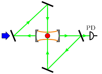
Figure 1: (Color online) The proposed experimental scheme. A two-level atom (red dot) is located in a leaky cavity which supports a single mode electromagnetic field. The photons outside the cavity can be reflected by the mirrors and serve as a common bath shared by the atom and the cavity. The photon detector (PD) is applied to detect the number of photons in the cavity.

The Hamiltonian of the global system can be written as the sum of three terms: $H=H_{JC}+H_{B}+H_{I}$, where

$$H_{JC} = \omega_{c}a^{\dagger}a+\frac{\omega_{0}}{2}\sigma_{z}+\lambda(a^{\dagger}\sigma^{-}+a\sigma^{+}),$$ (1a)

$$H_{B} = \sum_{i}\omega_{i}b_{i}^{\dagger}b_{i},$$ (1b)

$$H_{I} = \sum_{i}\kappa_{i}(ab_{i}^{\dagger}+b_{i}a^{\dagger})+\sum_{i}\xi_{i}(\sigma^{-}b_{i}^{\dagger}+b_{i}\sigma^{+}).$$ (1c)

The first term $H_{JC}$ is the Hamiltonian of our system, the JCM, which describes a two-level atom interacting with the single mode cavity photon under the rotating wave approximation. In Eq. (1a), $\omega_{c}$ is the frequency of the cavity mode, $a$ is the annihilation operator of the mode. The two energy levels of the atom are denoted as $|g\rangle$ and $|e\rangle$, and $\omega_{0}$ is the energy difference. The Pauli operators are defined as $\sigma_{z}\equiv|e\rangle\langle{e}|-|g\rangle\langle{g}|$, $\sigma^{-}\equiv|g\rangle\langle{e}|$, and $\sigma^{+}\equiv|e\rangle\langle{g}|$. $\lambda$ is the coupling strength between the atom and the cavity mode.

The second term $H_{B}$ describes the free terms of the photons in the ring cavity, which act as a bath in our scheme. In Eq. (1b), $\omega_{i}$ is the frequency of the $i$-th mode in the ring cavity and $b_{i}$ is its annihilation operator.

The third term $H_{I}$ describes the interactions between the system and the bath. In Eq. (1c), $\kappa_{i}$ ($\xi_{i}$) is the coupling strength between the atom (the cavity photons) and the $i$-th mode of the bath.

Now, we study how the photon in the cavity mode decays into the bath. Notice that there are two decay channels for the cavity photons. The cavity photons can either directly decay into the bath or be absorbed by the atom and decay into the bath through the atomic spontaneous emission . An intuitive idea is to sum the effects of the two channels fn and the master equation can be formally written as

$$\dot{\rho}=-i[H,\rho]+J_{1}(\omega_{c})\mathcal{L}[a]+J_{2}(\omega_{0})\mathcal{L}[\sigma^{-}],$$ (2)

where $\mathcal{L}[Q]=(2Q\rho Q^{\dagger}-Q^{\dagger}Q\rho-\rho Q^{\dagger}Q)$, and the spectrum functions $J_{1}(\omega)$ and $J_{2}(\omega)$ are defined as  aj ; hefeng

$$J_{1}(\omega) = \pi\sum_{j}\kappa_{j}^{2}\delta(\omega-\omega_{j}),$$ (3a)

$$J_{2}(\omega) = \pi\sum_{j}\xi_{j}^{2}\delta(\omega-\omega_{j}).$$ (3b)

However, the cavity mode and the atom share a common bath, and the quantum interference between the two decay channels is completely neglected in Eq. (2).

To take into account the interference effect, we need to reformulate the master equation. To this end, we first diagnose the Hamiltonian $H_{JC}$ for the the atom-cavity system. The ground state of $H_{JC}$ is a product state $|G\rangle=|0;g\rangle$ with eigen-energy $E_{0}=-\omega_{c}/2$. In the resonance case ($\omega_{c}=\omega_{0}$), the energies for the excited states are

$$E_{n}^{\pm}=(n-1/2)\omega_{c}\pm\lambda\sqrt{n},$$ (4)

and the corresponding eigen-vectors are the dressed states $|n,\pm\rangle=\left(\pm|n;g\rangle+|n-1;e\rangle\right)/\sqrt{2}$, which are coherent superpositions of the product states $|n;g\rangle$ and $|n-1;e\rangle$. Then the master equation can be derived under the Markov and secular approximations with the standard steps. The detailed derivation is shown in Ref. ct , the final result is obtained as

$$\dot{\rho}_{cd}=-i(E_{c}-E_{d})\rho_{cd}+\sum_{k,l}\gamma^{cdkl}\rho_{kl}$$ (5)

where $|c\rangle,|d\rangle,|k\rangle,|l\rangle$ are the dressed states of $H_{JC}$ with the eigen-energies $E_{c},E_{d},E_{k}$ and $E_{l}$ respectively, $\rho_{cd}=\langle c|\rho|d\rangle$ and $\rho_{kl}=\langle k|\rho|l\rangle$ are the elements of the reduced density matrix for the atom-cavity system. In Eq. (5), $\gamma^{cdkl}\equiv\sum_{i=1}^{4}\gamma_{i}$ with

$$\gamma_{1} = -\sum_{n}\left[J_{1}(\omega_{kn})\delta_{dl}a_{cn}^{\dagger}a_{nk}+J_{2}(\omega_{kn})\delta_{dl}\sigma_{cn}^{+}\sigma_{nk}^{-}+\sqrt{J_{1}(\omega_{kn})J_{2}(\omega_{kn})}\delta_{dl}\left(a_{cn}^{\dagger}\sigma_{nk}^{-}+\sigma_{cn}^{+}a_{nk}\right)\right]$$ (6a)

$$\gamma_{2} = J_{1}(\omega_{kc})a_{ck}a_{ld}^{\dagger}+J_{2}(\omega_{kc})\sigma_{ck}^{-}\sigma_{ld}^{+}+\sqrt{J_{1}(\omega_{kc})J_{2}(\omega_{kc})}\left(a_{ck}\sigma_{ld}^{+}+\sigma_{ck}^{-}a_{ld}^{\dagger}\right)$$ (6b)

$$\gamma_{3} = -\sum_{n}\left[J_{1}(\omega_{ln})\delta_{ck}a_{ln}^{\dagger}a_{nd}+J_{2}(\omega_{ln})\delta_{ck}\sigma_{ln}^{+}\sigma_{nd}^{-}+\sqrt{J_{1}(\omega_{ln})J_{2}(\omega_{ln})}\delta_{ck}\left(a_{ln}^{\dagger}\sigma_{nd}^{-}+\sigma_{ln}^{+}a_{nd}\right)\right]$$ (6c)

$$\gamma_{4} = J_{1}(\omega_{ld})a_{ck}a_{ld}^{\dagger}+J_{2}(\omega_{ld})\sigma_{ck}^{-}\sigma_{ld}^{+}+\sqrt{J_{1}(\omega_{ld})J_{2}(\omega_{ld})}\left(a_{ck}\sigma_{ld}^{+}+\sigma_{ck}^{-}a_{ld}^{\dagger}\right)$$ (6d)

where $\omega_{ij}=E_{i}-E_{j}$ is the energy difference between levels $i$ and $j$, and $A_{\alpha\beta}\equiv\langle\alpha|A|\beta\rangle$ is the matrix element of operator $A$ in the dressed state representation of the JCM. In the above equations, the terms proportional to $\sqrt{J_{1}(\cdot)J_{2}(\cdot)}$ represent the contribution from the quantum interference between the two decay channels.

Under the Ohmic dissipation, the spectrum functions $J_{1}(\omega)$ and $J_{2}(\omega)$ of the bath are expressed as

$$J_{1}(\omega) = 2\pi\alpha_{1}\omega\exp(-\omega/\omega_{c1}),$$ (7a)

$$J_{2}(\omega) = 2\pi\alpha_{2}\omega\exp(-\omega/\omega_{c2}),$$ (7b)

where $\alpha_{1(2)}$ is the dissipation coefficients and $\omega_{c1(c2)}$ denotes the cutoff frequencies.

In the end of this section, we point out the following two aspects. Firstly, the size of the external cavity in our consideration is in the order of $10cm$ jwpan , while the inner cavity is in the order of $nm$ to $\mu m$. Therefore, the external cavity is much larger than the inner cavity, and can support a lot of electromagnetic modes, which can be regarded as the environment. Although the photon mode in the inner cavity and the photons modes in the environment are all the bosonic modes, the coupling between the atom and photon mode in the inner cavity is much stronger than that between the atom and the environment, so we first diagnose the Hamiltonian of the system ($H_{JC}$) exactly, and regard the system-environment interaction as a perturbation safely and apply the Markov approximation to discuss the dynamics of the system. In Fig. 2, we plot the average photons number in the inner cavity as a function of the evolution time $t$ assuming the system is prepared in the state $|1;g\rangle\otimes|\bf{0}\rangle$ initially, with $|\bf{0}\rangle$ representing that all of the bath modes are in their vacuum states. For comparison, we also plot the results obtained by neglecting the interference effect (that is omitting the terms proportional to $\sqrt{J_{1}(\cdot)J_{2}(\cdot)}$ in Eqs. (6)) and the curve obtained from the traditional master equation (Eq. (2)). It is shown that, our results (secular) coincide with the numerical results perfectly, which confirms the effectiveness of Markov approximation. Besides, it is clearly shown that the interference effect dramatically slows down the decay of the whole system. The reason comes from the slow decaying of the anti-symmetry dressed state $|1-\rangle$, whose decay behavior is clearly shown in Sec. IV and the appendix. Secondly, only the bath modes which have the eigen frequencies around those of the lowest dressed states couple to the system and the coupling strength is much weaker than the atom-cavity coupling, i.e. $\lambda\gg\alpha_{1},\alpha_{2}$. As a result, the system will maintain enough coherence for a long time. As shown in Fig. 2, it exhibites an obvious oscillation for the evolution time $\omega_{c}t<200$ under our parameters.

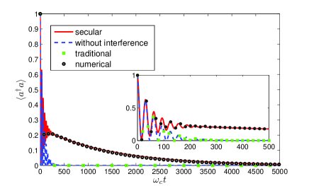
Figure 2: (Color online) The average photons number in the inner cavity as a function of the evolution time assuming the system is prepared in the state $|1;g\rangle\otimes|\bf{0}\rangle$ initially. The inset is the zoomed-in views. The parameters are set as $\omega_{0}=\omega_{c}=1,\lambda=0.1,\omega_{c1}=5,\omega_{c2}=8,\alpha_{1}=0.002,\alpha_{2}=0.001.$

III Quasi-dark state

In this section, we firstly turn off the interaction between the two level atom and the cavity mode, that is $\lambda=0$. Then, the master equation (5) degenerates into a simple expression

$$\dot{\rho} = -i[\omega_{c}a^{\dagger}a+\frac{\omega_{0}}{2}\sigma_{z},\rho]$$ (8)

$$+J_{1}[2a\rho a^{\dagger}-a^{\dagger}a\rho-\rho a^{\dagger}a]$$

$$+J_{2}[2\sigma^{-}\rho\sigma^{+}-\sigma^{+}\sigma^{-}\rho-\rho\sigma^{+}\sigma^{-}]$$

$$+\sqrt{J_{1}J_{2}}[2a\rho\sigma^{+}-\sigma^{+}a\rho-\rho\sigma^{+}a]$$

$$+\sqrt{J_{1}J_{2}}[2\sigma^{-}\rho a^{\dagger}-a^{\dagger}\sigma^{-}\rho-\rho a^{\dagger}\sigma^{-}],$$

where we write $J_{1}(\omega_{c})$ as $J_{1}$ and $J_{2}(\omega_{0})$ as $J_{2}$ for simple.

We prepare the system in the product state $|1;g\rangle\otimes|\bf{0}\rangle$ or $|0;e\rangle\otimes|\bf{0}\rangle$ initially and investigate the dynamical evolution of the system. Solving the above equation, we plot the curve of the average photons in the inner cavity $\langle a^{\dagger}a\rangle$ and the probability of the atom in its excited state $\langle|e\rangle\langle{e}|\rangle$ as a function of the evolution time in Fig. 3.

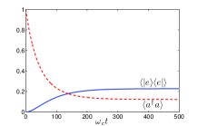
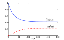
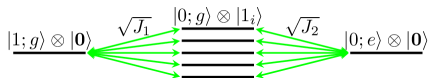
Figure 3: (Color online) The average photons in the inner cavity and the probability for the atom in its excited state as a function of evolution time $t$ with the initial state being (a)$|1;g\rangle\otimes|\bf{0}\rangle$ and (b)$|0;e\rangle\otimes|\bf{0}\rangle$ respectively. (c) The sketch of the energy level transitions of the system. The parameters are set as $\omega_{c}=\omega=1$, $\lambda=0$, $\omega_{c1}=5$, $\omega_{c2}=8$, $\alpha_{1}=0.002$, $\alpha_{2}=0.001$.

It is shown in the figure, the system will achieve a steady state dependent of its initial state instead of the thermal state equilibrium with the bath. If the system is prepared in the state $|1;g\rangle\otimes|\bf{0}\rangle$ initially, it satisfies

$$\langle a^{\dagger}a\rangle_{s}^{(g)} = \frac{J_{2}^{2}}{(J_{1}+J_{2})^{2}}$$ (9a)

$$\langle|e\rangle\langle e|\rangle_{s}^{(g)} = \frac{J_{1}J_{2}}{(J_{1}+J_{2})^{2}}$$ (9b)

where $\langle A\rangle_{s}^{(g)}$ denotes the average value of the operator $A$ over the steady state with the initial state being $|1;g\rangle\otimes|\bf{0}\rangle$. On the contrary, if the system is prepared in the state $|0;e\rangle\otimes|\bf{0}\rangle$ initially, it satisfies

$$\langle a^{\dagger}a\rangle_{s}^{(e)} = \frac{J_{1}J_{2}}{(J_{1}+J_{2})^{2}}$$ (10a)

$$\langle|e\rangle\langle e|\rangle_{s}^{(e)} = \frac{J_{1}^{2}}{(J_{1}+J_{2})^{2}}$$ (10b)

These results can be understood from a simple physical picture as shown in Fig. 3(c). The bath couples the two transition arms $|1;g\rangle\otimes|{\bf 0}\rangle\leftrightarrow|0;g\rangle\otimes|1_{i}\rangle$ and $|0;e\rangle\otimes|{\bf 0}\rangle\leftrightarrow|0;g\rangle\otimes|1_{i}\rangle$ simultaneously, where $|1_{i}\rangle$ represents that the $ith$ mode in the environment excites a photon, while the other modes are in their vacuum states. Generally speaking, only the near resonant bath modes contribute to the dynamics of the system, and the coupling intensities can be regarded as constants for these bath modes in the Ohmic spectrum situation. Furthermore, a discretization of Eq. (3) gives that the coupling intensities of the two arms are proportional to $\sqrt{J_{1}}$ and $\sqrt{J_{2}}$, respectively (as shown in Fig. 3(c)). The destructive interference between the two transitions occurs when the atom resonates with the cavity mode and the atom-cavity system may be trapped in the excited states

$$|D\rangle=\frac{\sqrt{J_{1}}|0;e\rangle-\sqrt{J_{2}}|1;g\rangle}{\sqrt{J_{1}+J_{2}}}$$ (11)

without decay even in the presence of the bath. The state $|D\rangle$ is similar to the dark state in EIT phenomenon which is implemented within the three-level or four-level systems, and we name it quasi-dark state. A straight calculation gives $\langle a^{\dagger}a\rangle_{s}^{(g)}=|\langle 1;g|D\rangle|^{2}|\langle D|1;g\rangle|^{2},\langle|e\rangle\langle e|\rangle_{s}^{(g)}=|\langle 1;g|D\rangle|^{2}|\langle D|0;e\rangle|^{2},\langle a^{\dagger}a\rangle_{s}^{(e)}=|\langle 0;e|D\rangle|^{2}|\langle D|1;g\rangle|^{2}$, as well as $\langle|e\rangle\langle e|\rangle_{s}^{(e)}=|\langle 0;e|D\rangle|^{2}|\langle D|0;e\rangle|^{2}$. Therefore, we conclude that the system will stay in the quasi-dark state with certain probability dependent of the initial state when it achieves steady state. In other words, the quasi-dark state prevents the system to reach the thermal state equilibrium with the bath.

Actually, the dark state of the system can be obtained in a more intuitive way. To this end, we rewrite the master equation Eq.(8) in a more simple expression:

$$\dot{\rho}=-i[H_{0},\rho]+\mathcal{L}[P]$$ (12)

where

$$H_{0}=\omega_{c}a^{\dagger}a+\frac{\omega_{0}}{2}\sigma_{z},$$ (13)

and

$$P=\sqrt{J_{1}}a+\sqrt{J_{2}}\sigma_{-}.$$ (14)

Since the dark state does not decay even in the dissipative system, it should be an eigenstate of $P$, we can directly write the dark state $|D\rangle$ as shown in Eq.(11), which is not only the eigen state of $P$ with a zero eigen value but satisfies that the corresponding density matrix commutes with the Hamiltonian $H_{0}$, and then $\dot{\rho}=0$. Physically speaking, it is the interference effect between the different dissipation channels that leads to the existence of the dark state. Arising from the same mechanism, the high fidelity dark entangled steady states can also be rapidly generated in interacting Rydberg atoms system DD .

IV Vacuum Rabi splitting

To further explore the effect of a common bath, we study the transmission spectrum of the system considering the direct atom-cavity coupling ($\lambda\neq 0$). To this aim, we drive the cavity by an external field and the action of the driven field on the cavity mode is described by

$$H_{driven}=\eta(a^{\dagger}e^{-i\omega_{d}t}+ae^{i\omega_{d}t})$$ (15)

where $\eta$ denotes the intensity of the driven field and $\omega_{d}$ its frequency.

The driven field induces the transition between the ground state and the excited states, while the dissipation causes the excited states to decay to the ground state. When the evolution time is long enough, the system may reach a steady state. To investigate the behavior of the steady state, we eliminate the time dependence from the Hamiltonian through the unitary transformation $U(t)=\exp[i(a^{\dagger}a+\sigma_{z}/2+\sum_{i}b_{i}^{\dagger}b_{i})\omega_{d}t]$. The atom-cavity Hamiltonian in the rotating frame becomes

$$\mathcal{H} = i\frac{\partial}{\partial t}U(t)U^{\dagger}(t)+U(t)\left(H_{JC}+H_{driven}\right)U^{\dagger}(t)$$

$$= \Delta_{1}a^{\dagger}a+\frac{\Delta_{2}}{2}\sigma_{z}+\lambda(a^{\dagger}\sigma^{-}+a\sigma^{+})+\eta(a^{\dagger}+a)$$

where $\Delta_{1(2)}=\omega_{c(0)}-\omega_{d}$ is the detuning between the cavity (atom) and the driven field. The last term can be regarded as a perturbation whenever $\eta\ll\omega_{c},\omega_{0},\lambda,$ i.e., weak driven field. Then the master equation can be written as

$$\frac{d}{dt}\rho_{cd}=-i\langle c[\mathcal{H},\rho]|d\rangle+\sum_{k,l}\gamma^{cdkl}\rho_{kl}.$$ (17)

Therefore, the average photon number over the steady state is obtained numerically by finding the density matrix satisfying $d\rho_{cd}/dt=0$ for any eigen states $|c\rangle$ and $|d\rangle$ of $H_{JC}$. The results are shown in Fig. 4, where the average photon number reaches its peaks when the driven field is just resonant with the energy difference between the dressed states $|1,\pm\rangle$ and the ground state $|G\rangle$. This effect is the vacuum Rabi splitting.

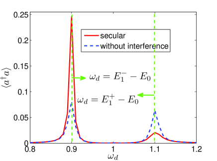
Figure 4: (Color online) The steady state of the system driven by an external field. The parameters are set as $\omega_{0}=\omega_{c}=1,\lambda=0.1,\omega_{c1}=5,\omega_{c2}=8,\alpha_{1}=0.002,\alpha_{2}=0.001,\eta=0.005.$

In Fig. 4, we also plot the results given by neglecting the contribution from quantum interference. It is shown that the double peaks exhibit an obvious asymmetric character if the quantum interference between two decay channels is taken into consideration. As observed, the peak corresponding to $\omega_{d}=E_{1}^{-}-E_{0}$ is elevated while the peak corresponding to $\omega_{d}=E_{1}^{+}-E_{0}$ is suppressed compared with the case that neglects the effect of quantum interference.

Now let us explain the physics underlying the exotic phenomenon and analysis how the quantum interference effect affects the decay rate of the dressed states in the following two steps.

Firstly, we neglect the interference between the two decay channels. That is, the atom and the cavity experience dissipation independently. As discussed above, the atom-cavity coupling dressed them and the eigen energies of the dressed states $|1,\pm\rangle$ are $\omega_{1,\pm}$. Following the master equation (5) and setting the terms proportional to $\sqrt{J_{1}(\cdot)J_{2}(\cdot)}$ to zero in Eqs. (6), the decay rate of the dressed states $|1,\pm\rangle$ are both the sum of the decay rate of the atom and the cavity mode, that is, $\Gamma^{1,\pm}=J_{1}(\omega_{1\pm,0})+J_{2}(\omega_{1\pm,0})$. In the case of Ohmic spectrum, it satisfied $\Gamma^{1,+}\approx\Gamma^{1,-}$, therefore, we obtain two nearly symmetrical peaks in Fig. 4.

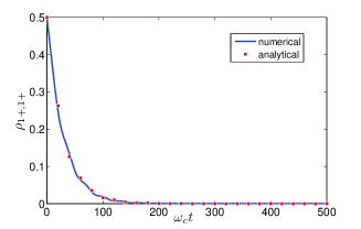
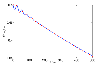
Figure 5: (Color online) The time evolution of matrix elements $\rho_{1+,1+}$ and $\rho_{1-,1-}$. The solid line: the numerical solution, The solid square: the analytical solution whose detail derivation is shown in the appendix. The parameters are set as $\omega_{0}=\omega_{c}=1$, $\lambda=0.1$, $\omega_{c1}=5,$ $\omega_{c2}=8$, $\alpha_{1}=0.002,$ $\alpha_{2}=0.001.$ The system is initially prepared in the state $|1;g\rangle\otimes|\bf{0}\rangle$.

Then, we furthermore consider the quantum interference between the two decay channels. Arising from the constructive interference, the decay rate of the symmetric dressed state $|1,+\rangle$ becomes $\big{(}\sqrt{J_{1}(\omega_{1+,0})}+\sqrt{J_{2}(\omega_{1+,0})}\big{)}^{2}$ which even surpasses the sum of the decay rate of subsystems. On contrary, due to the destructive interference, the decay rate of the antisymmetric dressed state $|1,-\rangle$ is $\big{(}\sqrt{J_{1}(\omega_{1-,0})}-\sqrt{J_{2}(\omega_{1-,0})}\big{)}^{2}$ which may even achieve $0$ under some special parameters (for example $J_{1}(\omega_{1-,0})=J_{2}(\omega_{1-,0})$). It implies that the antisymmetry state will have an infinite lifetime.

The above analysis implies that the symmetric dressed state $|1,+\rangle$ has a much larger decay rate than that of the antisymmetric dressed state $|1,-\rangle$. The same conclusion is also shown in Fig. 5, where we plot the probability for the system in the symmetric and antisymmetric dressed states (the time evolution of the density matrix elements $\rho_{1+,1+}$ and $\rho_{1-,1-}$), assuming the system is prepared in the state $|1;g\rangle\otimes|\bf{0}\rangle$ initially. It is clearly that the symmetric state $|1,+\rangle$ decays more faster than the antisymmetric state $|1,-\rangle$. Apart from the numerical result, an analytical result based on iteration calculations is shown in the appendix.

Now, the asymmetric vacuum Rabi splitting can be explained from the different decay rates of the states $|1,+\rangle$ and $|1,-\rangle$. Because the state $|1,-\rangle$ has a smaller decay rate, the steady state will have a larger component. This will give a stronger signal of the average photon number. In contrary, the state $|1,+\rangle$ has a larger decay rate, so the steady state will have a smaller component and it will give a weaker signal.

As is well known, the eigen states of the JC model consist a bare ground state and pairs of dressed states, which are anti-symmetric and symmetric states when the cavity mode is resonant with the atom. From the above discussions, it can be concluded that any anti-symmetric dressed state $|n,-\rangle$ for both $n=1$ and $n\neq 1$ will have a smaller decay rate than the corresponding symmetric dressed state $|n,+\rangle$.

Actually, the same asymmetric Rabi splitting is also given when the two level atom is replaced by a single mode harmonic oscillator. This similarity can be clarified by investigating the low energy levels of the system. To this end, we write the Hamiltonian of coupled resonant oscillators as

$$H_{co} = \omega a^{\dagger}a+b^{\dagger}b+\lambda(a^{\dagger}b+b^{\dagger}a)$$ (18)

$$= (\omega+\lambda)A^{\dagger}A+(\omega-\lambda)B^{\dagger}B.$$

where $a$ and $b$ are the annihilation operators for the two coupled oscillators respectively, and the new set of bosonic operators $A,B$ are defined as $A=(a+b)/\sqrt{2}$ and $B=(a-b)/\sqrt{2}$. Diagnosing the Hamiltonian $H_{co}$ when the coupling strength is smaller than the frequencies of the oscillators ($\lambda<\omega$), the eigen energies can be obtained as

$$E_{m_{1},m_{2}}=m_{1}(\omega+\lambda)+m_{2}(\omega-\lambda)$$ (19)

where $m_{1}$ and $m_{2}$ are integers. It is obvious that energies of the first three energy levels are $E_{0,0}=0,E_{0,1}=\omega-\lambda,E_{1,0}=\omega+\lambda$ and the splitting is $E_{1,0}-E_{0,1}=2\lambda$ which is same as that of the JC model. Therefore, we will obtain similar asymmetric peaks in the transmission spectrum at zero temperature.

However, the higher energy levels of the coupled oscillators (as shown in Eq. (19)) are much different from those of the JC model which are shown in Eq. (4). Therefore, the splitting will behave differently in the two systems in finite temperature.

V Conclusions and remarks

In this paper, we discuss the dissipation of the interacting atom-cavity system when the atom and the cavity mode share a common bath. We regard the spectrum of the environment as Ohmic spectrum which is the major decoherence source often found in the qubit’s environment aj ; uw . We can also choose other type environment, but the quantum interference effect will not be changed quantitatively. To investigate the effect of the common bath, we reformulated the master equation and obtained simple expressions as shown in Eqs. (8,12). Actually, it can also be written as the form of Fokker-Planck equation in coherence state representation carmichael . Solving the Fokker-Planck equation, we need not to truncate the photons number and it is convenient to deal with the system with large Hilbert space. However, it includes no more physics than the operator form of the master equation because they are indeed the same equations in different representations.

In summary, we have proposed a scheme to realize the JCM with a common bath within the current experimental capabilities. In our system, the common bath induces a quasi-dark state which does not decay and prevents the system to equilibrate with the bath. Besides, the decay processes of the atom and the cavity interfere with each other and the constructive interference leads the symmetric dressed state decaying much faster than the antisymmetric dressed state. As a result, the vacuum Rabi splitting in the transmission spectrum shows an obvious asymmetric character. Furthermore, the robustness of the antisymmetric dressed state may be applied in quantum information process, such as the storage of the quantum state in quantum network.

Appendix A The iteration solution for $\rho_{1+,1+}$ and $\rho_{1-,1-}$

In the main text, we have solved the master equation numerically and obtained the time evolution of the matrix elements $\rho_{1+,1+}$ and $\rho_{1-,1-}$ as shown in Fig. 4. Now, we will give some analytical results based on the iteration calculation. To this end, we restrict our consideration in no excitation and only one excitation subspaces which are spanned by the ground state $|G\rangle$ and the dressed states $|1,\pm\rangle$ of the JCM. Then, Utilizing the master Eq. (4) in the main text, the equations for $\rho_{1\pm,1\pm}$ are written as

$$\dot{\rho}_{1+,1+} = \gamma^{1+,1+,1+,1+}\rho_{1+,1+}+\gamma^{1+,1+,1+,1-}\rho_{1+,1-}$$ (20a)

$$+\gamma^{1+,1+,1-,1+}\rho_{1-,1+},$$

$$\dot{\rho}_{1-,1-} = \gamma^{1-,1-,1-,1-}\rho_{1-,1-}+\gamma^{1-,1-,1+,1-}\rho_{1+,1-}$$ (20b)

$$+\gamma^{1-,1-,1-,1+}\rho_{1-,1+},$$

$$\dot{\rho}_{1+,1-} = -i(\omega_{1+}-\omega_{1-})\rho_{1+,1-}+\gamma^{1+,1-,1+,1-}\rho_{1+,1-}$$

$$+\gamma^{1+,1-,1+,1+}\rho_{1+,1+}+\gamma^{1+,1-,1-,1-}\rho_{1-,1-},$$

$$\dot{\rho}_{1-,1+} = -i(\omega_{1-}-\omega_{1+})\rho_{1-,1+}+\gamma^{1-,1+,1-,1+}\rho_{1-,1+}$$

$$+\gamma^{1-,1+,1+,1+}\rho_{1+,1+}+\gamma^{1-,1+,1-,1-}\rho_{1-,1-}.$$

Now, we solve the matrix elements $\rho_{1+,1+}$ and $\rho_{1-,1-}$ in two steps. Firstly, we neglect the dependence on $\rho_{1+,1+}$ and $\rho_{1-,1-}$ of $\rho_{1+,1-}$ and $\rho_{1-,1+}$, that is, the last two terms in Eq. (LABEL:1p1n) and Eq. (LABEL:1n1p). Then we obtain

$$\rho_{1+,1-} = \rho_{1+,1-}(0)e^{[\gamma^{1+,1-,1+,1-}-i(\omega_{1+}-\omega_{1-})]t}$$ (21a)

$$\rho_{1-,1+} = \rho_{1-,1+}(0)e^{[\gamma^{1-,1+,1-,1+}+i(\omega_{1+}-\omega_{1-})]t}$$ (21b)

Secondly, substituting the last two equations back into Eq. (20a) and Eq. (20b), we finally obtain the matrix elements $\rho_{1+,1+}$ and $\rho_{1-,1-}$ as

$$\rho_{1+,1+} = \left[\begin{array}[]{c}\gamma^{1+,1+,1+,1-}\rho_{1+,1-}(0)\frac{\exp\{[\gamma^{1+,1-,1+,1-}-\gamma^{1+,1+,1+,1+}-i(\omega_{1+}-\omega_{1-})]t\}-1}{\gamma^{1+,1-,1+,1-}-\gamma^{1+,1+,1+,1+}-i(\omega_{1+}-\omega_{1-})}\\ +\gamma^{1+,1+,1-,1+}\rho_{1-,1+}(0)\frac{\exp\{[\gamma^{1-,1+,1-,1+}-\gamma^{1+,1+,1+,1+}+i(\omega_{1+}-\omega_{1-})]t\}-1}{\gamma^{1-,1+,1-,1+}-\gamma^{1+,1+,1+,1+}+i(\omega_{1+}-\omega_{1-})}\\ +\rho_{1+,1+}(0)\end{array}\right]e^{\gamma_{1+,1+,1+,1+}t}$$ (22d)

$$\rho_{1-,1-} = \left[\begin{array}[]{c}\gamma^{1-,1-,1+,1-}\rho_{1+,1-}(0)\frac{\exp\{[\gamma^{1+,1-,1+,1-}-\gamma^{1-,1-,1-,1-}-i(\omega_{1+}-\omega_{1-})]t\}-1}{\gamma^{1+,1-,1+,1-}-\gamma^{1-,1-,1-,1-}-i(\omega_{1+}-\omega_{1-})}\\ +\gamma^{1-,1-,1-,1+}\rho_{1-,1+}(0)\frac{\exp\{[\gamma^{1-,1+,1-,1+}-\gamma^{1-,1-,1-,1-}+i(\omega_{1+}-\omega_{1-})]t\}-1}{\gamma^{1-,1+,1-,1+}-\gamma^{1-,1-,1-,1-}+i(\omega_{1+}-\omega_{1-})}\\ +\rho_{1-,1-}(0)\end{array}\right]e^{\gamma_{1-,1-,1-,1-}t}.$$ (22h)

where we have defined $\gamma s$ in the main text. In Fig. 5 ,we find that the results from the iteration calculation agree with numerical results very well.

References

• (1) H. P. Breuer and F. Petruccione, The Theory of Open Quantum Systems (Oxford University Press, Oxford, London, 2002).
• (2) V. Braginsky and F. Khalili, Quantum Measurement (Cambridge University Press, London, 1992).
• (3) G. M. Huang, T. J. Tarn, and J. W. Clark, J. Math. Phys. 24, 2608 (1983).
• (4) M. A. Nielsen and I. L. Chuang, Quantum Computation and Quantum Information (Cambridge University Press, Cambridge, U.K., 2000).
• (5) V. Ramakrishna and H. Rabitz, Phys. Rev. A 54, 1715 (1996).
• (6) X. H. Bao, A. Reingruber, P. Dietrich, J. Rui, A. Duck, T. Strassel, L. Li, N. L. Liu, B. Zhao, and J. W. Pan, Nature Phys. 8, 512 (2012)
• (7) A. J. Leggett, S. Chakravarty, A. T. Dorsey, M. P. A. Fisher, A. Garg, and W. Zwerger, Rev. Mod. Phys. 59, 1 (1987).
• (8) U. Weiss, Quantum Dissipative Systems, third Edition, (World Scientific Publishing, 2008).
• (9) T. Yu and J. H. Eberly, Phys. Rev. Lett. 93, 140404 (2004).
• (10) D. Braun, Phys. Rev. Lett. 89, 277901 (2002).
• (11) J. Ma, Z. Sun, X. G. Wang, and F. Nori, Phys. Rev. A 85, 062323 (2012).
• (12) J. Li and G. S. Paraoanu, New J. Phys. 11, 113020 (2009).
• (13) J. Q. Liao, J. F. Huang, and L. M. Kuang, Phys. Rev. A 83, 052110 (2011).
• (14) S. W. Li, L. P. Yang, and C. P. Sun, Arxiv. 1303, 1266v1 (2013).
• (15) T. H$\ddot{\mathrm{a}}$yrynen, J. Oksanen, and J. Tulkki, Phys. Rev. A 83, 013801 (2011).
• (16) A. Stokes, A. Kurcz, T. P. Spiller, and A. Beige, Phys. Rev. A 85, 053805 (2012).
• (17) L. S. Bishop, E. Ginossar, and S. M. Girvin, Phys. Rev. Lett. 105, 100505 (2010).
• (18) M. Scala, B. Militello, A. Messina, J. Piilo, and S. Maniscalco, Phys. Rev. A 75, 013811 (2007).
• (19) M. J. Bhaseen, J. Mayoh, B. D. Simons, and J. Keeling, Phys. Rev. A 85, 013817 (2012).
• (20) B. Masashi, J. Phys. A: Math. Theor. 43, 335305 (2010).
• (21) G. Gangopadhyay, S. Basu, and D. S. Ray, Phys. Rev. A 47, 1314 (1993).
• (22) C. Cohen-Tannouji, J. Dupont-Roc, and G. Grynberg, Atom-Photon Interactions: Basic Process and Applications(John,Wiley & Sons,New York,1998).
• (23) S. E. Harris, Phys. Today 50, 36 (1997).
• (24) E. T. Jaynes and F. W. Cummings, Proc IEEE 51,89 (1963).
• (25) T. H$\ddot{\mathrm{u}}$mmer, G. M. Reuther, P. H$\ddot{\mathrm{a}}$nggi, and D. Zueco, Phys. Rev. A 85, 052320 (2012).
• (26) F. Nissen, S. Schmidt, M. Biondi, G. Blatter, H. E. T$\ddot{\mathrm{u}}$reci, and J. Keeling, Phys. Rev. Lett. 108, 233603 (2012).
• (27) G. S. Agarwal, Phys. Rev. Lett. 57, 1732 (1984).
• (28) R. J. Thompson, G. Rempe, and H. J. Kimble, Phys. Rev. Lett. 68, 1132 (1992).
• (29) Y. F. Zhu, D. J. Gauthier, S. E. Morin, Q. L. Wu, H. J. Carmichael, and T. W. Mossberg, Phys. Rev. Lett. 64, 2499 (1990).
• (30) S. Savasta, R. Saija, A.Ridolfo, O. D. Stefano, P. Denti, and F. Borghese, ACS. Nano. 4, 6369 (2010).
• (31) T. Yoshie, A. Scherer, J. Hendrickson, G. Khitrova, H. M. Gibbs, G. Rupper, C. Ell, O. B. Shchekin, and D. G. Deppe, Nature, 432, 200 (2004).
• (32) H. Toida, T. Nakajima, and S. Komiyama, Phys. Rev. Lett. 110, 066802 (2013).
• (33) F. Galve, G. L. Giorgi, and R. Zambrini, Phys. Rev. A 81, 062117 (2010)
• (34) H. F. Wang, S. Ashhab, and F. Nori, Phys. Rev. A 83, 062317 (2011).
• (35) D. D. Bhaktavatsala Rao and K. Mølmer, Phys. Rev. Lett. 111, 033606 (2013).
• (36) H. J. Carmichael, Statistical Methods in Quantum Optics I (Springer, 1999)