Two unconditionally implied parameters and volatility smiles and skews

Abstract

The paper studies estimation of parameters of diffusion market models from historical data. The standard definition of implied volatility for these models presents its value as an implicit function of several parameters, including the risk-free interest rate. In reality, the risk free interest rate is unknown and need to be forecasted, because the option price depends on its future curve. Therefore, the standard implied volatility is conditional: it depends on the future values of the risk free rate. We study two implied parameters: the implied volatility and the implied average cumulative risk free interest rate. They can be found unconditionally from a system of two equations. We found that very simple models with random volatilities (for instance, with two point distributions) generate various volatility smiles and skews with this approach.
Key words: market models, parameters estimation, Black-Scholes, implied volatility, implied forward risk-free rate, volatility smile, volatility skew

Short running head: Two unconditionally implied parameters

Introduction

Most practitioners have adapted the famous Black-Scholes model as the premier model for pricing and hedging of options. This model consists of two assets: the risk free bond or bank account and the risky stock. It is assumed that the dynamics of the stock is given by a random process with some standard deviation of the stock returns (the volatility coefficient, or volatility). Empirical research shows that the real volatility is time-varying and random. Many authors emphasize that the main difficulty in modifying the Black–Scholes and Merton models is taking into account this fact. A number of equations for evolution of the volatility were proposed (see e.g. Christie (1982), Johnson and Shanno (1987), Hull and White (1987), Masi et al. (1994), and more recent papers in Jarrow (ed.) (1998)). The basic pricing rule for models with random volatility is risk neutral valuation, when the option price is given as the expected value of its future payoff with respect to a risk-neutral measure discounted back to the present time $t$ (see, e.g., Ross (1976) and Cox and Ross (1976)). This method has been developed to pricing rules based on optimal choice of the risk-neutral measures such as local risk minimization, mean variance hedging, $q$-optimal measures, and minimal entropy measures (see, e.g., Föllmer and Sondermann (1986), Schweizer (1992), Masi et al. (1994), Geman et al. (1995), Rheinländer and Schweizer (1997), Pham et al. (1998), Laurent and Pham (1999), Frittelli (2000), and others). These pricing rules are applicable for the most complicated models with Itô’s equation for volatility.

In reality, practitioners prefer to describe market imperfection and deviations from log-normal Black-Scholes model in the terms of the so-called volatility smile or volatility skew for the implied volatility. It is a certain shape of the implied volatility on $K$ given $S(0)$, where $K$ is the strike price, $S(0)$ is the stock price; $\cup$-shape is usually referred as the volatility smile, $\cap$-shape and others are referred as the volatility skew. It is commonly recognized that Black-Scholes formula gives unbiased estimation for at-money options only, and it gives a systematic error for in-money and out-of-money options. That means that there is a gap between historical and implied volatility that generates volatility smile or skew (see, e.g. Black and Scholes (1972), Day and Levis (1992), Derman et al. (1996), Hauser and Lauterbach (1997), Taylor and Xu (1994). A detailed review can be found in Mayhew (1995)). Therefore, there is a demand for models consisting of stock prices, option prices, and volatilities, that can cover different shapes of volatility smiles and skews. For instance, the risk neutral valuation method generates volatility smiles rather than skews.

In the present paper, we found a very simple model with random volatilities and risk free rates (for instance, with two point distributions) that generates various volatility smiles and skews. Our approach can be described as the following. The standard implied volatility definition gives its value as a function of the risk-free interest rate $r$, the option price, the strike price, the current stock price, and terminal time $T$. The standard definition of the implied volatility ignores the fact that, in reality, $r$ is unknown and need to be forecasted, because the option price depends on its future (forward) curve. Therefore, the standard implied volatility at time $t$ is a conditional one and it depends on the future curve $r(s)|_{s\in[t,T]}$. In fact, the Black-Scholes price at time $t$ depends only the volatility process and on $\rho(t)=(T-t)^{-1}\int_{t}^{T}r(s)ds$, or on a single parameter of this curve (see Lemma 1.1 below), even if $r(\cdot)$ is random and depends on $(S,\sigma,w)$, where $w$ s the driving Wiener process. We suggest to calculate the pair $(\sigma_{imp}(t),\rho_{imp}(t))$ of two unconditionally implied parameters, where $\sigma_{imp}(t)$ is the unconditionally implied volatility, and $\rho_{imp}(t)$ is the unconditionally implied value of $\rho(t)$. This pair can be found from a system of two equations with option prices for different strike prices. Note that the case when two parameters are inferred from option historical prices has been addressed by several authors but in different setting (see, e.g., survey of Garcia et al (2004)). Butler and Schachter (1996) suggested to use two call options with different strike prices for calculation of implied volatility distributions for the case of option prices obtained via the unbiased estimate of option price for random volatility. The mentioned paper addressed the case of implied risk-free rate, but it was focused on the case of the implied stock prices and volatility.

Our main goal is a model for volatility skews and smiles. Using numerical simulation, we show that even simplest models with the random volatility and the risk free rate with two point distributions generate various volatility smiles and skews.

1 Definitions

We consider the diffusion model of a securities market consisting of a risk free bond or bank account with the price $B(t),$ ${t\geq 0}$, and a risky stock with price $S(t)$, ${t\geq 0}$. The prices of the stocks evolves as

$$dS(t)=S(t)\left(a(t)dt+\sigma(t)dw(t)\right),\quad t>0,$$ (1.1)

where $w(t)$ is a Wiener process, $a(t)$ is an appreciation rate, $\sigma(t)$ is a random volatility coefficient. The initial price $S(0)>0$ is a given deterministic constant. The price of the bond evolves as

$$B(t)=\exp\biggl{(}\int_{0}^{t}r(s)ds\biggr{)}B(0),$$ (1.2)

where $r(t)\geq 0$ is a random process and $B(0)$ is given.

We assume that $w(\cdot)$ is a standard Wiener process on a given standard probability space $(\Omega,{\cal F},{\bf P})$, where $\Omega$ is a set of elementary events, ${\cal F}$ is a complete $\sigma$-algebra of events, and ${\bf P}$ is a probability measure.

Let ${\cal F}_{t}$ be a filtration generated by the currently observable data. We assume that the process $(S(t),\sigma(t))$ is ${\cal F}_{t}$-adapted and that ${\cal F}_{t}$ does not depend on $\{w(t_{2})-w(t_{1})\}_{t_{2}\geq t_{2}\geq t}$. In particular, this means that the process $(S(t),\sigma(t))$ is currently observable and $\sigma(t)$ does not depend on $\{w(t_{2})-w(t_{1})\}_{t_{2}\geq t_{2}\geq t}$. We assume that ${\cal F}_{0}$ is the $P$-augmentation of the set $\{\emptyset,\Omega\}$, and that $a(t)$ does not depend on $\{w(t_{2})-w(t_{1})\}_{t_{2}\geq t_{2}\geq t}$. For simplicity, we assume that $a(t)$ is a bounded process.

Black-Scholes price

Let $K>0$ be given. We shall consider two types of options: vanilla call and vanilla put, with payoff function $f(S(T))=F(S(T),K)$, where $F(S(T),K)=(S(T)-K)^{+}$ or $F(S(T),K)=(K-S(T))^{+}$, respectively. Here $K$ is the strike price.

Let $T>0$ be fixed. Let $H_{{\scriptscriptstyle BS},c}(t,x,\sigma,r,K)$ and $H_{{\scriptscriptstyle BS},p}(t,x,\sigma,r,K)$ denotes Black-Scholes prices for the vanilla put and call options with the payoff functions $F(S(T),K)$ described above under the assumption that $S(t)=x$, $(\sigma(s),r(s))=(\sigma,r)$ $(\forall s>t)$, where $\sigma\in(0,+\infty)$ is non-random. The Black-Scholes formula for call can be rewritten as

$$H_{{\scriptscriptstyle BS},c}(t,x,\sigma,r,K)=x\Phi(d_{+}(t,x,\sigma,r,K))-Ke^{-r(T-t)}\Phi(d_{-}(t,x,\sigma,r,K)),$$ (1.3)

$$H_{{\scriptscriptstyle BS},p}(t,x,\sigma,r,K)=H_{{\scriptscriptstyle BS},c}(t,x,\sigma,r,K)-x+Ke^{-r(T-t)},$$

where

$$\Phi(x)\stackrel{{\scriptstyle{\scriptscriptstyle\Delta}}}{{=}}\frac{1}{\sqrt{2\pi}}\int_{-\infty}^{x}e^{-\frac{s^{2}}{2}}ds,$$

and where

$$d_{+}(x,t,\sigma,r,K) \stackrel{{\scriptstyle{\scriptscriptstyle\Delta}}}{{=}} \frac{\log{(x/K)}+(T-t)r}{\sigma\sqrt{(T-t)}}+\frac{\sigma\sqrt{(T-t)}}{2},$$

$$d_{-}(x,t,\sigma,r,K) \stackrel{{\scriptstyle{\scriptscriptstyle\Delta}}}{{=}} d_{+}(x,t,\sigma,r,K)-\sigma\sqrt{(T-t)}.$$ (1.4)

Set

$$\tilde{S}(t)\stackrel{{\scriptstyle{\scriptscriptstyle\Delta}}}{{=}}S(t)\exp\biggl{(}-\int_{0}^{t}r(s)ds\biggr{)}.$$

We assume that there exist a risk-neutral measure $Q$ such that the process $\tilde{S}(t)$ is a martingale under $Q$, i.e., ${\bf E}_{Q}\{\tilde{S}(T)\,|{\cal F}_{t}\}=\tilde{S}(t)$, where ${\bf E}_{Q}$ is the corresponding expectation.

For brevity, we shall denote by $H_{{\scriptscriptstyle BS}}$ the corresponding Black-Scholes prices different options, i.e., $H_{{\scriptscriptstyle BS}}=H_{{\scriptscriptstyle BS},c}$ or $H_{{\scriptscriptstyle BS}}=H_{{\scriptscriptstyle BS},p}$, for vanilla call, vanilla put respectively. Let

$$v(t)\stackrel{{\scriptstyle{\scriptscriptstyle\Delta}}}{{=}}\frac{1}{T-t}\int_{t}^{T}\sigma(s)^{2}ds,\quad\rho(t)\stackrel{{\scriptstyle{\scriptscriptstyle\Delta}}}{{=}}\frac{1}{T-t}\int_{t}^{T}r(s)ds.$$

The following lemma is a generalization for random $r(\cdot)$ of the lemma from Hull and White (1987), p.245.

Lemma 1.1

Let $t\in[0,T)$ be fixed. Let $v(t)$ and $\rho(t)$ be ${\cal F}_{t}$-measurable. Then

$${\bf E}_{{Q}}\{e^{-\int_{t}^{T}r(s)ds}F(S(T))|{\cal F}_{t}\}=H_{{\scriptscriptstyle BS}}(t,S(t),\sqrt{v(t)},\rho(t),K).$$

Clearly, $\frac{1}{T-t}\int_{t}^{T}\sigma(s)^{2}ds$ and $\frac{1}{T-t}\int_{t}^{T}r(s)ds$ are not ${\cal F}_{t}$-measurable in the general case of stochastic $(r,\sigma)$, and the assumptions of Lemma 1.1 are not satisfied.

Proof of Lemma 1.1. It suffices to consider the case when $t=0$ and $v(0)$ and $\rho(0)$ are non-random.

Set $\tilde{K}\stackrel{{\scriptstyle{\scriptscriptstyle\Delta}}}{{=}}K\exp\biggl{(}-\int_{0}^{T}r(s)ds\biggr{)}.$ We introduce the function $\widehat{H}_{\scriptscriptstyle BS}(\cdot):[0,T]\times{\bf R}\to{\bf R}$ such that

$$e^{\rho(0)t}\widehat{H}_{{\scriptscriptstyle BS}}(t,x)\equiv H_{{\scriptscriptstyle BS}}(t,e^{\rho(0)t}x,\sqrt{v(0)},\rho(0),K).$$

It is easy to see that

$$\begin{array}[]{ll}\frac{\partial\widehat{H}_{{\scriptscriptstyle BS}}}{\partial t}(t,x)+\frac{1}{2}v(0)x^{2}\frac{\partial^{2}\widehat{H}_{{\scriptscriptstyle BS}}}{\partial x^{2}}(t,x)=0,\\ \widehat{H}_{{\scriptscriptstyle BS}}(T,x)=F(x,\tilde{K}).\end{array}$$

Let

$$\tau(t)\stackrel{{\scriptstyle{\scriptscriptstyle\Delta}}}{{=}}\frac{1}{v(0)}\int_{0}^{t}\sigma(s)^{2}ds,\quad\tilde{X}(t)\stackrel{{\scriptstyle{\scriptscriptstyle\Delta}}}{{=}}\tilde{H}_{{\scriptscriptstyle BS}}(\tau(t),\tilde{S}(t)),\quad\tilde{S}(t)\stackrel{{\scriptstyle{\scriptscriptstyle\Delta}}}{{=}}\exp\left(\int_{0}^{t}r(s)ds\right)S(t).$$

By Ito formula, we obtain that

$$d\tilde{X}(t)=\frac{\partial\widehat{H}_{{\scriptscriptstyle BS}}}{\partial x}(\tau(t),\tilde{S}(t))d\tilde{S}(t),\quad\tilde{X}(T)=F(\tilde{S}(T),\tilde{K}).$$

Hence

$$\tilde{X}(0)=\widehat{H}_{{\scriptscriptstyle BS}}(0,S(0))={\bf E}_{Q}F(\tilde{S}(T),\tilde{K})={\bf E}_{Q}\exp\left(-\int_{0}^{T}r(s)ds\right)F(S(T),K).$$

This completes the proof. $\Box$

Corollary 1.1

Assume that $H_{{\scriptscriptstyle BS}}=H_{{\scriptscriptstyle BS},c}$, or $H_{{\scriptscriptstyle BS}}=H_{{\scriptscriptstyle BS},p}$, or $H_{{\scriptscriptstyle BS}}=H_{{\scriptscriptstyle BS},s}$. Consider a market model with pricing rule (1.6). Let $(\sigma,r)$ does not depend on $w$ under ${Q}$. Then $P_{{\scriptscriptstyle RN}}(t)={\bf E}_{Q}\{H_{{\scriptscriptstyle BS}}(t,S(t),\sqrt{v(t)},\rho(t),K)\,|\,{\cal F}_{t}\}$, where $(v,\rho)$ are defined in Lemma 1.1.

Unconditionally implied parameters

The standard definition of the implied volatility ignores the fact that, in reality, $r$ is unknown and need to be forecasted, because the option price depends on its future (forward) curve. Therefore, the standard implied volatility at time $t$ is a conditional one and it depends on the future curve $r(s)|_{s\in[t,T]}$. We shall study the pair $(\sigma_{imp}(t),\rho_{imp}(t))$ of two unconditionally implied parameters, where $\sigma_{imp}(t)$ is the unconditionally implied volatility, and $\rho_{imp}(t)$ is the unconditionally implied value of $\rho(t)$. This pair of implied parameters can be inferred from a system of two equations for different options.

Definition 1.1

Assume that we observe two options on the same stock with market prices $P^{(1)}(t)$ and $P^{(2)}(t)$ at time $t$. These options have the same expiration time $T>0$. Let $H_{{\scriptscriptstyle BS}}^{(1)}$ and $H_{{\scriptscriptstyle BS}}^{(2)}$ be the Black-Scholes price for the corresponding types of options. Let the pair $(\sigma_{{\scriptscriptstyle imp}}(t),\rho_{{\scriptscriptstyle imp}}(t))$ be such that

$$\left\{\begin{array}[]{ll}H_{{\scriptscriptstyle BS}}^{(1)}(t,S(t),\sigma_{{\scriptscriptstyle imp}}(t),\rho_{{\scriptscriptstyle imp}}(t))=P^{(1)}(t),\\ H_{{\scriptscriptstyle BS}}^{(2)}(t,S(t),\sigma_{{\scriptscriptstyle imp}}(t),\rho_{{\scriptscriptstyle imp}}(t))=P^{(2)}(t).\end{array}\right.$$ (1.5)

We say that $\sigma_{{\scriptscriptstyle imp}}(t)$ is the implied volatility and $\rho_{{\scriptscriptstyle imp}}(t)$ is the implied average forward risk-free rate inferred from (1.5).

To avoid technical difficulties, we shall assume that the prices and parameters in (1.5) are such that the solution $(\sigma_{{\scriptscriptstyle imp}}(t),\rho_{{\scriptscriptstyle imp}}(t))$ exists and is uniquely defined for all special case described below. Clearly, Definition 1.1 is model free and does not require any pricing rules and a prior assumptions on the evolution law for volatilities and risk free rates. We need some models and pricing rules only for numerical simulations of of $(\sigma_{{\scriptscriptstyle imp}}(t),\rho_{{\scriptscriptstyle imp}}(t))$.

Pricing rule

The local risk minimization method, the mean variance hedging, and some other methods based on the risk-neutral valuation lead to the following pricing rule: given $(a,\sigma,r)$, the option price is

$$P_{{\scriptscriptstyle RN}}(t,\sigma(\cdot),r(\cdot))\stackrel{{\scriptstyle{\scriptscriptstyle\Delta}}}{{=}}{\bf E}_{Q}\{e^{-\int_{t}^{T}r(s)ds}F(S(T))\,|\,{\cal F}_{t}\},$$ (1.6)

where $Q$ is some risk neutral measure, and where ${\bf E}_{Q}$ is the corresponding expectation. Usually, $Q$ is uniquely defined by $(a,\sigma,r)$, and by the pricing method used.

For numerical simulation purposes, we assume that we have chosen one of these methods (for instance, local risk minimization method or mean variance hedging). Therefore, the risk neutral measure $Q$ is uniquely defined by $(a,\sigma,r)$ given the method of pricing.

2 Two calls with different strike prices

Assume that two European call options on the same stock have market prices $P_{i}(t)$ at time $t$, $i=1,2$. We assume that these options have the same expiration time $T>0$ and have different strike prices $K_{i}>0$, $K_{1}\neq K_{2}$. Let $\sigma_{{\scriptscriptstyle imp}}(t)=\sigma_{{\scriptscriptstyle imp}}(t,K_{1},K_{2})$ be the implied volatility and $\rho_{{\scriptscriptstyle imp}}(t)=\rho_{{\scriptscriptstyle imp}}(t,K_{1},K_{2})$ be the implied average forward risk-free rate given $K_{1},K_{2}$ at time $t$, inferred from the system

$$\left\{\begin{array}[]{ll}H_{{\scriptscriptstyle BS},c}(t,S(t),\sigma_{{\scriptscriptstyle imp}}(t),\rho_{{\scriptscriptstyle imp}}(t),K_{1})=P_{1}(t),\\ H_{{\scriptscriptstyle BS},c}(t,S(t),\sigma_{{\scriptscriptstyle imp}}(t),\rho_{{\scriptscriptstyle imp}}(t),K_{2})=P_{2}(t).\end{array}\right.$$ (2.1)

Remark 2.1

For solution of system (3.1), the following straightforward algorithm can be applied. Let $\sigma_{1}(t,K_{1}|\,\rho)$ be such that

$$H_{{\scriptscriptstyle BS},c}(t,S(t),\sigma_{1}(t,K_{1}|\,\rho),\rho,K_{1})=P_{1}(t).$$

(i.e. it is the standard (conditional) implied volatility). Consider equation

$$H_{{\scriptscriptstyle BS},c}(t,S(t),\sigma_{1}(t,K_{1}|\,\rho),\rho,K_{2})=P_{2}(t).$$ (2.2)

Let $\widehat{\rho}=\widehat{\rho}(K_{1},K_{2})$ be the solution of (2.2). Then

$$(\sigma_{{\scriptscriptstyle imp}}(t),\rho_{{\scriptscriptstyle imp}}(t))=\left(\sigma_{1}(t,K_{1}|\,\widehat{\rho}(K_{1},K_{2})),\widehat{\rho}(K_{1},K_{2})\right).$$

Numerical simulation for generic market model

For numerical simulation, we accept the simplest stock market model with traded options on that stock and with pricing rule (1.6). Assume that the risk neutral measure $Q$ is such that the process $(r(t),\sigma(t))=(\sigma,r)$ is random, independent on $w$ under $Q$, independent on time, and can take only two values, $(r_{1},\sigma_{1})$ and $(r_{2},\sigma_{2})$, with probabilities $p$ and $1-p$ correspondingly, where $p\in[0,1]$ is given. In that case, pricing rule (1.6) means that the price of call option with strike price $K$ and expiration time $T$ is

$${\bf E}_{Q}\max(0,\tilde{S}_{T}-\tilde{K})=p\,H_{{\scriptscriptstyle BS}}(T,S_{0},r_{1},\sigma_{1},K)+(1-p)\,H_{{\scriptscriptstyle BS}}(T,S_{0},r_{2},\sigma_{2},K).$$

Clearly, any $p\in[0,1]$ defines its own risk-neutral probability measure $Q$, and, therefore, it defines its own ${\bf E}_{Q}$.

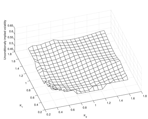
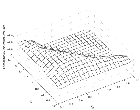
Figure 4.1: Unconditionally implied volatility $\sigma_{{\scriptscriptstyle imp}}(t,K_{1},K_{2})$ (top) and average forward risk-free rate (bottom) $r_{{\scriptscriptstyle imp}}(t,K_{1},K_{2})$ inferred from prices for two call options for the case when $t=0$, $T=1$, $S(0)=1$, $p=0.5$, $\sigma_{1}=0.3$, $\sigma_{2}=0.7$, $r_{1}=0.01$, $r_{2}=0.08$.

As an example, we consider the case when $t=0$, $T=1$, $S(0)=1$, $p=0.5$, $\sigma_{1}=0.3$, $\sigma_{2}=0.7$, $r_{1}=0.1$, $r_{2}=0.08$. Figure 4.1 shows the unconditionally implied volatility and average forward risk-free rate $(\sigma_{{\scriptscriptstyle imp}}(t,K_{1},K_{2}),r_{{\scriptscriptstyle imp}}(t,K_{1},K_{2}))$

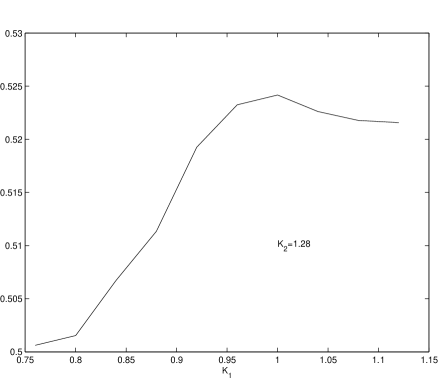
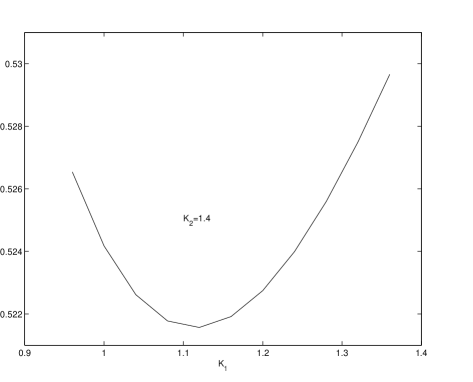
Figure 4.2: Unconditionally implied volatility $\sigma_{{\scriptscriptstyle imp}}(t,K_{1},K_{2})$ inferred from prices for two call options given $K_{2}=1.28$ and $K_{2}=1.4$.

Figure 4.2 shows the shape of dependence of unconditionally implied volatility $\sigma_{{\scriptscriptstyle imp}}(t,K_{1},K_{2})$ on $K_{1}$ given $K_{2}=1.28$ and $K_{2}=1.4$.

It can be seen that the volatility surface the risk-free rate surface neither convex nor concave with respect to $(K_{1},K_{2})$, and our simplest model can generate volatility smiles as well as skews.

3 Exclusion of the stock prices form the system of equation

For the dynamic estimation of time varying implied parameters, one has to separate the impact of the changes of the stock price on the option price from the impact of the change of the values of the stock price parameters. For this, it could be convenient to exclude the current stock price form the system of equations for the implied parameters. To address it, we suggest the following approach.

Let us consider dynamically adjusted parameters $T=t+\tau$ and $K=\kappa S(t)$, where $\kappa\in(0,+\infty)$ is a parameter. In this case, $F(S(T))=F(S(T),K)=S(t)F(Y(t+\tau),\kappa)$, where

$$Y(T)=S(t+\tau)/S(t).$$

By rule (1.6), the option price given $(a,\sigma,r)$, is

$$P_{{\scriptscriptstyle RN}}(t,\sigma(\cdot),r(\cdot)) \stackrel{{\scriptstyle{\scriptscriptstyle\Delta}}}{{=}} {\bf E}_{Q}\{e^{-\int_{t}^{T}r(s)ds}F(S(T),K)\,|\,{\cal F}_{t}\}$$

$$= S(t){\bf E}_{Q}\{e^{-\int_{t}^{t+\tau}r(s)ds}F(Y(t+\tau),\kappa)\,|\,{\cal F}_{t}\},$$

where $Q$ is some risk neutral measure, and where ${\bf E}_{Q}$ is the corresponding expectation.

Let

$$G(t)\stackrel{{\scriptstyle{\scriptscriptstyle\Delta}}}{{=}}\frac{P_{{\scriptscriptstyle RN}}(t,\sigma(\cdot),r(\cdot))}{S(t)}.$$

It follows that

$$G(t)={\bf E}_{Q}\{e^{-\int_{t}^{t+\tau}r(s)ds}F(Y(t+\tau),\kappa)\,|\,{\cal F}_{t}\},$$

Therefore, the implied parameters $(\sigma_{{\scriptscriptstyle imp}}(t),\rho_{{\scriptscriptstyle imp}}(t))$ for European options can be calculated using $H_{{\scriptscriptstyle BS}}(t,1,\sigma,\rho,\delta)$ only with $\kappa=\kappa_{i}$, $i=1,2$, $\kappa_{1}\neq\kappa_{2}$.

Let us consider the following example. Assume that two European call options on the same stock have market prices $P_{i}(t)$ at time $t$, $i=1,2$. We assume that these options have the same expiration time $T=t+\tau>0$ and have different strike prices $K_{i}=\kappa_{i}S(t)>0$, $\kappa_{1}\neq\kappa_{2}$. Let $G_{i}(t)=P_{i}(t)/S(t)$. In this case, the implied volatility $\sigma_{{\scriptscriptstyle imp}}(t)$ and the  implied average forward risk-free rate $\rho_{{\scriptscriptstyle imp}}(t)$ at time $t$ can be inferred from the system

$$\left\{\begin{array}[]{ll}H_{{\scriptscriptstyle BS},c}(t,1,\sigma_{{\scriptscriptstyle imp}}(t),\rho_{{\scriptscriptstyle imp}}(t),\kappa_{1})=G_{1}(t),\\ H_{{\scriptscriptstyle BS},c}(t,1,\sigma_{{\scriptscriptstyle imp}}(t),\rho_{{\scriptscriptstyle imp}}(t),\kappa_{2})=G_{2}(t).\end{array}\right.$$ (3.1)

Remark 3.1

The observations of option prices with dynamic adjusted strike price $K=\kappa S(t)$ with a fixed $\kappa$ can be useful for econometrics purposes even without calculation of the implied parameters. In particular, some features of the evolution law for historical parameters $(\sigma(t),\rho(t))$ can be restored directly from the observations of the process $G(t)$. For instance, the processes $G(t)$ must evolve as a deterministic function of the current values of $(\sigma(t),\rho(t))$ if the process $(\sigma(t),\rho(t))$ evolves as a Markov process that is independent from $w(\cdot)$.

4 Possible generalizations

The approach suggested in this paper allows many straightforward generalizations. For instance, assume that implied parameters are calculated using market prices of three options with expiration times $T_{1},T_{2},T_{3}$ such that $T_{1}<T_{2}=T_{3}$. Let $\sigma_{1},\sigma_{2},\sigma_{3},\rho$ be the corresponding implied volatilities and the implied cumulative risk free rate calculated as the solution of the system of the three equations for prices; we assume that $\sigma_{2}=\sigma_{3}$. The relationship between $\sigma_{1}$ and $\sigma_{2}=\sigma_{3}$ shows the implied market hypothesis about the evolution of the volatility.

Furthermore, sets of special implied parameters can be used for models that are different from the Black-Scholes diffusion market model. For example, consider a model with driving fractional Brownian motion with unknown Hurst parameter $h$. A system of three equations including the prices for three options can be used to determine the implied $(\rho,\sigma,h)$, where $\rho$ is the implied risk-free rate, $\sigma$ is the implied risk-free rate, $h$ is the implied Hurst parameter. Instead of the classical Black-Scholes formula for the prices, one should use the corresponding modification of the pricing formula for the case of fractional Brownian motion.

The same approach for can be applied for the discrete time market models. Let us consider the so-called binomial model. Let us suggest an example of a pair of implied parameters associated with a modification of this model with the prices $S(t)$, $t=0,1,2,...,N$. We assume that the evolution of $S(t)$ is such that $S(t+1)=\rho S(t)\zeta(t+1)$, $t=0,1,2,...$, where ${\bf P}(\zeta(t+1)\in\{1-\varepsilon,(1-\varepsilon)^{-1}\}|{\cal F}_{t})=1$, where ${\cal F}_{t}$ is the filtration generated by $S(t)$, $\rho\geq 1$ is the single period return for the risk free investment, $\varepsilon\in(0,1)$ is a parameter for the model. Instead of the classical Black-Scholes formula for the option price, one can use the value of the initial wealth that allows replication of the claim $\rho^{-N}F(S(N))$. The pair $(\rho,\varepsilon)$ can be used as the pair of implied parameters; $\rho$ represents the single period return for the risk-free investment, and $\varepsilon$ represents the range of change that can be considered as an analog of the volatility.

For the classical binomial model, the sets of all possible values of the stock prices are finite at every time. Let us suggest a modification of the discrete time binomial model such that the distribution of the stock price is continuous and the stock prices can take any positive value. Let us consider first a model for ”rounded” prices $S_{0}(t)$ with a finite set of possible values at any time $t=0,1,2,...$. We assume that the evolution of $S_{0}(t)$ is described by a standard discrete time binomial model such that $S_{0}(0)=1$, $S_{0}(t+1)=\rho S(t)\zeta(t+1)$, $t=0,1,2,...$, where ${\bf P}(\zeta(t+1)\in\{1-\varepsilon,(1-\varepsilon)^{-1}\}|{\cal F}_{t})=1$, ${\cal F}_{t}$ is the filtration generated by $S_{0}(t)$, $\rho\geq 1$ is the single period return for the risk free investment, $\varepsilon\in(0,1)$ is a parameter for the model. Second, let us consider a sequence of random variables $\xi(t,v)$ such that are mutually independent given ${\cal F}_{t}$ and that they all have the uniform distribution on $[(1-\varepsilon),(1-\varepsilon)^{-1}]$ conditionally given ${\cal F}_{t}$, where $v\in V_{t}$. Here $V_{t}$ is the supporting set for the distribution of $S_{0}(t)$ . Finally, let us select the final model for the stock prices to be $S(t+1)=\rho S(t)\zeta(t+1)\xi(t+1,S_{0}(t))$. For this model, $S(t)$ can take any positive value. The pair $(\rho,\varepsilon)$ can be used as the pair of implied parameters again; instead of the Black-Scholes pricing formula, one can use the price calculated for the binomial stock price model described by $S_{0}(t)$.

The author wishes to thank Barry Schachter for useful comments regarding the bibliography.

References

     Black, F. and M. Scholes (1972): The valuation of options contracts and test of market efficiency. Journal of Finance, 27, 399-417.

Butler, J.S. and B. Schachter (1996): Statistical Properties of Parameters Inferred from the Black-Scholes Formula August. International Review of Financial Analysis 5, 223-235.

Christie, A. (1982): The stochastic behavior of common stocks variances: values, leverage, and interest rate effects. Journal of Financial Economics, 10, 407-432.

Day, T.E. and C.M. Levis (1992): Stock market volatility and the information content of stock index options. Journal of Econometrics, 52, 267-287.

Cox, J. C., and S.A. Ross (1976): The valuation of options for alternative stochastic processes, Journal of Financial Economics 3, 145 166.

Derman, E., I. Kani, and J.Z. Zou (1996): The local volatility surface: unlocking the information in index option prices. Financial Analysts Journal 25-36.

Geman, H. and T. Ane (1996): Stochastic subordination. Risk, 9 (9), 145-149.

Fleming, W., and H.M. Soner (1993): Controlled Markov Processes and Viscosity Solutions. Applications Math., vol. 25. Berlin-Heidelberg-New York: Springer.

Föllmer, H., and D. Sonderman (1986): Hedging of Non-Redundant Contingent Claims. In: Mas-Colell, A., Hildebrand, W. (eds.) Contributions to Mathematical Economics. Amsterdam: North Holland 1986, pp. 205 223.

Frittelli, M. (2000): The minimal entropy martingale measure and the valuation problem in incomplete markets. Mathematical Finance, 10, 39- 52.

Geman H., N.El Karoui, J.-C.Rochet. (1995): Changes of numeraire, changes of probability measure and option pricing. Journal of Applied Probability 32 443-458.

Garcia, R., Ghysels, E., Renault, E. (2004): The Econometrics of option pricing, Working Paper CIRANO 2004s-04 (to appears in Handbook of Financial Econometrics, Y. Ait-Sahalia and L.P. Hansen (eds.) North Holland).

Hauser, S. and B. Lauterbach (1997): The relative performance of five alternative warrant pricing models. Financial Analysts Journal, N1, 55-61.

Hull, J. and A. White (1987): The pricing of options on assets with stochastic volatilities. Journal of Finance, 42, 281-300.

Jarrow, R. (ed.) (1998): Volatility New Estimations Techniques for pricing Derivatives, Risk Books.

Johnson, H. and D. Shanno (1987): Option pricing when the variance is changing. Journal of Financial and Quantitative Analysis, 22, 143-151.

Lambertone, D., and B. Lapeyre (1996): Introduction to Stochastic Calculus Applied to Finance. London: Chapman & Hall.

Laurent, J.P., and H. Pham (1999): Dynamic programming and mean-variance hedging. Finance and Stochastics 3, 83 110.

Masi, G.B., Kabanov, Yu.M., and W.J. Runggaldier (1994): Mean-variance hedging of options on stocks with Markov volatilities. Theory of Probability and Its Applications 39, 172-182.

Mayhew, S. (1995): Implied volatility. Financial Analysts Journal, iss. 4, 8-20.

Pham, H., Rheinlander, T., and M. Schweizer (1998): Mean-variance hedging for continuous processes: new proofs and examples. Finance and Stochastics 2, 173–198.

Rheinländer, T., and M. Schweizer (1997): On $L^{2}$-projections on a space of stochastic integrals. Annals of Probability 25, 1810-1831.

Ross, S. (1976): Options and efficiency, Quarterly Journal of Economics 90, 75 89.

Schweizer, M. (1992): Mean-Variance Hedging for General Claims. Annals of Applied Probability 2, 171-179.

Taylor, S.J. and X. Xu (1994): The magnitude of implied volatility smiles: theory and empirical evidence for exchange rates. Review of Future Markets, 13, 355-380.