Stochastic Modeling of Large-Scale Solid-State Storage Systems: Analysis, Design Tradeoffs and Optimization

Abstract

Solid state drives (SSDs) have seen wide deployment in mobiles, desktops, and data centers due to their high I/O performance and low energy consumption. As SSDs write data out-of-place, garbage collection (GC) is required to erase and reclaim space with invalid data. However, GC poses additional writes that hinder the I/O performance, while SSD blocks can only endure a finite number of erasures. Thus, there is a performance-durability tradeoff on the design space of GC. To characterize the optimal tradeoff, this paper formulates an analytical model that explores the full optimal design space of any GC algorithm. We first present a stochastic Markov chain model that captures the I/O dynamics of large-scale SSDs, and adapt the mean-field approach to derive the asymptotic steady-state performance. We further prove the model convergence and generalize the model for all types of workload. Inspired by this model, we propose a randomized greedy algorithm (RGA) that can operate along the optimal tradeoff curve with a tunable parameter. Using trace-driven simulation on DiskSim with SSD add-ons, we demonstrate how RGA can be parameterized to realize the performance-durability tradeoff.

1 Introduction

The increasing adoption of solid-state drives (SSDs) is revolutionizing storage architectures. Today’s SSDs are mainly built on NAND flash memory, and provide several attractive features: high performance in I/O throughput, low energy consumption, and high reliability due to their shock resistance property. As the SSD price per gigabyte decreases [21], not only desktops are replacing traditional hard-disk drives (HDDs) with SSDs, but there is a growing trend of using SSDs in data centers [19, 27].

SSDs have inherently different I/O characteristics from traditional HDDs. An SSD is organized in blocks, each of which usually contains 64 or 128 pages that are typically of size 4KB each. It supports three basic operations: read, write, and erase. The read and write operations are performed in a unit of page, while the erase operation is performed in the block level. After a block is erased, all pages of the block become clean. Each write can only operate on a clean page; when a clean page is written, it becomes a valid page. To improve the write performance, SSDs use the out-of-place write approach. That is, to update data in a valid page, the new data is first written to a different clean page, and the original page containing old data is marked invalid. Thus, a block may contain a mix of clean pages, valid pages, and invalid pages.

The unique I/O characteristics of SSDs pose different design requirements from those in HDDs. Since each write must operate on a clean page, garbage collection (GC) must be employed to reclaim invalid pages. GC can be triggered, for example, when the number of clean pages drops below a predefined threshold. During GC, some blocks are chosen to be erased, and all valid pages in an erased block must first be written to a different free block prior to the erasure. Such additional writes introduce performance overhead to normal read/write operations. To maintain high performance, one design requirement of SSDs is to minimize the cleaning cost, such that a GC algorithm chooses blocks containing as few valid pages as possible for reclamation.

However, SSDs only allow each block to tolerate a limited number of erasures before becoming unusable. For instance, the number is typically 100K for single-level cell (SLC) SSDs and 10K for multi-level cell (MLC) SSDs [13]. With more bits being stored in a flash cell and smaller feature size of flash cells, the maximum number of erasures tolerable by each block further decreases, for example, to several thousands or even several hundreds for the latest 3-bits MLC SSDs [23]. Thus, to maintain high durability, another design requirement of SSDs is to maximize wear-leveling in GC, such that all blocks should have similar numbers of erasures over time so as to avoid any “hot” blocks being worn out soon.

Clearly, there is a performance-durability tradeoff in the GC design space. Specifically, a GC algorithm with a low cleaning cost may not achieve efficient wear-leveling, or vice versa. Prior work (e.g., [1]) addressed the tradeoff, but the study is mainly based on simulations. From the viewpoints of SSD practitioners, it remains an open design issue of how to choose the “best” parameters of a GC algorithm to adapt to different tradeoff requirements for different application needs. However, understanding the performance-durability tradeoff is non-trivial, since it depends on the I/O dynamics of an SSD and the dynamics characterization becomes complicated with the increasing numbers of blocks/pages of the SSD. This motivates us to formulate a framework that can efficiently capture the optimal design space of GC algorithms and guide the choices of parameterizing a GC algorithm to fit any tradeoff requirement.

In this paper, we develop an analytical model that characterizes the I/O dynamics of an SSD and the optimal performance-durability tradeoff of a GC algorithm. Using our model as a baseline, we propose a tunable GC algorithm for different performance-durability tradeoff requirements. To summarize, our paper makes the following contributions:

• We formulate a stochastic Markov chain model that captures the I/O dynamics of an SSD. Since the state space of our stochastic model increases with the SSD size, we adapt the mean field technique [5, 37] to make the model tractable. We formally prove the convergence results under the uniform workload to enable us to analyze the steady-state performance of a GC algorithm. We also discuss how our system model can be extended for a general workload.

• We identify the optimal extremal points that correspond to the minimum cleaning cost and the maximum wear-leveling, as well as the optimal tradeoff curve of cleaning cost and wear-leveling that enables us to explore the full optimal design space of the GC algorithms.

• Based on our analytical model, we propose a novel GC algorithm called the randomized greedy algorithm (RGA) that can be tunable to operate along the optimal tradeoff curve. RGA also introduces low RAM usage and low computational cost.

• To address the practicality of our work, we conduct extensive simulations using the DiskSim simulator [8] with SSD extensions [1]. We first validate via synthetic workloads that our model efficiently characterizes the asymptotic steady-state performance. Furthermore, we consider real-world workload traces and use trace-driven simulations to study the performance tradeoff and versatility of RGA.

The rest of the paper proceeds as follows. In §2, we propose a Markov model to capture the system dynamics of an SSD and conduct the mean field analysis. We formally prove the convergence, and further extend the model for a general workload. In §3, we study the design tradeoff between cleaning cost and wear-leveling of GC algorithms. In §4, we propose RGA and analyze its performance. In §5, we validate our model via simulations. In §6, we present the trace-driven simulation results. In §7, we review related work, and finally in §8, we conclude the paper.

2 System Model

We formulate a Markov chain model to characterize the I/O dynamics of an SSD under the read, write, and GC operations. We then analyze the model via the mean field technique when the SSD scales with the increasing number of blocks or storage capacity.

2.1 Markov Chain Model Formulation

Our model considers an SSD with $N$ blocks of $k$ pages each, where the typical value of $k$ is 64 or 128 for today’s commonly used SSDs. Since SSDs use the out-of-place write approach (see §1), a write to a logical page may reflect on any physical page. Therefore, SSDs implement address mapping to map a logical page to a physical page. Address mapping is maintained in the software flash translation layer (FTL) in the SSD controller. It can be implemented in block level [42], page level [24], or hybrid form [16, 33, 39]. A survey of the FTL design including the address mapping mechanisms can be found in [17]. In this paper, our model abstracts out the complexity due to address mapping; specifically, we focus on the physical address space and directly characterize the I/O dynamics of physical blocks.

Recall from §1 that a page can be in one of the three states: clean, valid or invalid. We classify each block into a different type based on the number of valid pages containing in the block. Specifically, a block of type $i$ contains exactly $i$ valid pages. Since each block has $k$ pages, a block can be of one of the $k\!+\!1$ types (i.e., from 0 to $k$ valid pages). If a block is of type $i$, then we say it is in state $i$. Let $X_{n}(t)$ denote the state of block $n\in\{1,...,N\}$ at time $t$. Then the state descriptor for the whole SSD is

$$\mbox{\boldmath$X$}^{N}(t)=(X_{1}(t),X_{2}(t),\ldots,X_{N}(t)),$$ (1)

where $X_{i}(t)\!\in\!\{0,1,...,k\}$. Thus, the state space cardinality is $(k\!+\!1)^{N}$. To facilitate our analysis under the large system regime (as we will show later), we transform the above state descriptor to:

$$\mbox{\boldmath$n$}^{N}(t)=(n_{0}(t),n_{1}(t),\ldots,n_{k}(t)),$$ (2)

where $n_{i}(t)\!\in\!\{0,1,...,N\}$ denotes the number of type $i$ blocks in the SSD. Clearly, we have $\sum_{j=0}^{k}\!n_{j}(t)\!=\!N$, and the state space cardinality is $\binom{N+k}{k}$.

We first describe how different I/O requests affect the system dynamics of an SSD from the perspective of physical blocks. The I/O requests can be classified into four types: (1) read a page, (2) perform GC on a block, (3) program (i.e., write) new data to a page, and (4) invalidate a page. First, read requests do not change $\mbox{\boldmath$n$}^{N}(t)$. For GC, the SSD selects a block, writes all valid pages of that block to a clean block, and finally erases the selected block. Thus, GC requests do not change the state of $\mbox{\boldmath$n$}^{N}(t)$ either. On the other hand, for the program and invalidate requests, if the corresponding block is of type $i$, it will move from state $i$ to state $i\!+\!1$ and to state $i\!-\!1$, respectively.

We now describe the state transition of a block in an SSD. Since the read and GC requests do not change $\mbox{\boldmath$n$}^{N}(t)$, we only need to model the program and invalidate requests. Suppose that the program and invalidate requests arrive as a Poisson process with rate $\lambda$. Also, suppose that the workload is uniform, such that all pages in the SSD will have an equal probability of being accessed (in §2.5, we extend our model for a general workload). The assumption of the uniform workload implies that (1) each block has the same probability $1/N$ of being accessed, (2) the probability of invalidating one page is proportional to the number of valid pages of the corresponding block, and (3) the probability of programming a page is proportional to the total number of invalid and clean pages of the corresponding block. Thus, if the requested block is of type $i$, then the probability of invalidating one page of the block is $\frac{i}{k}$, and that of programming one page in the block is $\frac{k-i}{k}$. Figure 1 illustrates the state transitions of a single block in an SSD under the program and invalidate requests. If a block is in state $i$, the program and invalidate requests will move it to state $i\!+\!1$ at rate $\frac{\lambda(k-i)}{Nk}$ and to state $i\!-\!1$ at rate $\frac{\lambda i}{Nk}$, respectively. Note that Figure 1 only shows the state transition of a particular block, but not the whole SSD. Specifically, the state space cardinality of a particular block is $k+1$ as shown in Figure 1, while that of the whole SSD is $\binom{N+k}{k}$ as described by Equation (2).

Figure 1: State transition of a block in an SSD.

To characterize the I/O dynamics of an SSD, we define the occupancy measure $\boldsymbol{M}^{N}(t)$ as the vector of fraction of type $i$ blocks at time $t$. Formally, we have

$$\boldsymbol{M}^{N}(t)=(M_{0}(t),M_{1}(t),...,M_{k}(t)),$$

where $M_{i}(t)$ is

$$M_{i}(t)=\frac{1}{N}\sum_{n=1}^{N}\mathbf{1}_{\{X_{n}(t)=i\}}=\frac{n_{i}(t)}{N}.$$ (3)

In other words, $M_{i}(t)$ is the fraction of type $i$ blocks in the SSD. It is easy to see that the occupancy measure $\boldsymbol{M}^{N}(t)$ is a homogeneous Markov chain.

We are interested in modeling large-scale SSDs to understand the performance implication of any GC algorithms. By large-scale, we mean that the number of blocks $N$ of an SSD is large. For example, for a 256GB SSD (which is available in many of today’s SSD manufactures), we have $N\!\approx\!1\!\times\!10^{6}$ and $k=64$ for a page size of 4KB, implying a huge state space of $\boldsymbol{M}^{N}(t)$. Since $\boldsymbol{M}^{N}(t)$ does not possess any special structure (i.e., matrix-geometric form), analyzing it can be computationally expensive.

2.2 Mean Field Analysis

To make our Markov chain model tractable for a large-scale SSD, we employ the mean field technique [5, 37]. The main idea is that the stochastic process $\boldsymbol{M}^{N}(t)$ can be solved by a deterministic process $\boldsymbol{s}(t)=(s_{0}(t),s_{1}(t),...,s_{k}(t))$ as $N\rightarrow\infty$, where $s_{i}(t)$ denotes the fraction of blocks of type $i$ at time $t$ in the deterministic process. We call $\boldsymbol{s}(t)$ the mean field limit. By solving the deterministic process $\boldsymbol{s}(t)$, we can obtain the occupancy measure of the stochastic process $\boldsymbol{M}^{N}(t)$.

We introduce the concept of intensity denoted by $\varepsilon(N)$. Intuitively, the probability that a block performs a state transition per time slot is in the order of $\varepsilon(N)$. Under the uniform workload, each block is accessed with the same probability $1/N$, so we have $\varepsilon(N)=1/N$. Now, we re-scale the process $\boldsymbol{M}^{N}(t)$ to $\widetilde{\boldsymbol{M}}^{N}(t)$.

$$\widetilde{\boldsymbol{M}}^{N}(t\varepsilon(N))=\boldsymbol{M}^{N}(t)\quad\forall t\geq 0.$$ (4)

For simplicity, we drop the notation $t$ when the context is clear. We now show how the deterministic process $\boldsymbol{s}(t)$ is related to the re-scaled process $\widetilde{\boldsymbol{M}}^{N}(t)$. The time evolution of the deterministic process can be specified by the following set of ordinary differential equations (ODEs):

$$\frac{ds_{i}}{dt}\!= -\lambda s_{i}\!+\!\lambda\frac{k\!-\!i\!+\!1}{k}s_{i\!-\!1}\!+\!\lambda\frac{i\!+\!1}{k}s_{i\!+\!1},\quad 1\!\leq\!i\!\leq\!k\!-\!1,$$ (5)

$$\frac{ds_{0}}{dt}\!= -\lambda s_{0}\!+\!\lambda\frac{1}{k}s_{1},$$

$$\frac{ds_{k}}{dt}\!= -\lambda s_{k}\!+\!\lambda\frac{1}{k}s_{k\!-\!1}.$$

The idea of the above ODEs is explained as follows. For an SSD with $N$ blocks, we express the expected change in number of blocks of type $i$ over a small time period of length $dt$ under the re-scaled process $\widetilde{\boldsymbol{M}}^{N}(t)$. This corresponds to the expected change over the time period of length $Ndt$ under the original process $\boldsymbol{M}^{N}(t)$. During this period (of length $Ndt$), there are $\lambda(Ndt)$ program/invalidate requests, each of which changes the state of some type $i$ block to state $i-1$ or state $i+1$ with probability $1/N$. Since there are a total of $Ns_{i}$ blocks of type $i$, the expected change from state $i$ to other states is $\lambda Ndts_{i}$. Using the similar arguments, the expected change in number of blocks from state $i\!+\!1$ to state $i$ is $\lambda Ndt\frac{i+1}{k}s_{i+1}$, and that from state $i-1$ to state $i$ is $\lambda Ndt\frac{k-i+1}{k}s_{i-1}$. Similarly, we can also specify the expected change in fraction of blocks of type $0$ and type $k$, and we obtain the ODEs as stated in Equation (5).

2.3 Derivation of the Fixed Point

We now derive the fixed point of the deterministic process in Equation (5). Specifically, $\boldsymbol{s}(t)$ is said to be a fixed point if $\boldsymbol{s}(t)=\boldsymbol{\pi}$ implies $\boldsymbol{s}(t^{\prime})=\boldsymbol{\pi}$ for all $t^{\prime}\geq t$. In other words, the fixed point $\boldsymbol{\pi}$ describes the distribution of different types of blocks in the steady state. The necessary and sufficient condition for $\boldsymbol{\pi}$ to be a fixed point is that $\frac{d\pi_{i}}{dt}=0$ for all $i\in\{0,1,\ldots,k\}$.

Theorem 1

Equation (5) has a unique fixed point $\boldsymbol{\pi}$ given by:

$$\pi_{i}=\frac{\binom{k}{i}}{2^{k}},\,0\leq i\leq k.$$ (6)

Proof: First, it is easy to check that $\boldsymbol{\pi}$ satisfies $\frac{d\pi_{i}}{dt}\!=\!0$ for $0\!\leq\!i\!\leq\!k$. Conversely, based on the condition of $\frac{d\pi_{i}}{dt}=0$ for all $i$, we have

$$-\pi_{i}\!+\!\frac{k-i+1}{k}\pi_{i-1}\!+\!\frac{i+1}{k}\pi_{i+1}=0,\quad 1\leq i\leq k\!-\!1,$$

$$-\pi_{0}\!+\!\frac{1}{k}\pi_{1}=0,$$

$$-\pi_{k}+\frac{1}{k}\pi_{k-1}=0.$$

By solving these equations, we get

$$\pi_{i}=\binom{k}{i}\pi_{k},\textrm{ for }0\leq i\leq k.$$

Since $\sum\limits_{i=0}^{k}\!\pi_{i}\!\!=\!\!1$, the fixed point is derived as in Equation (6).  

2.4 Summary

We develop a stochastic Markov chain model to characterize the I/O dynamics of a large-scale SSD system. Specifically, we solve the stochastic process with a deterministic process via the mean field technique and identify the fixed point in the steady state. We claim that the derivation is accurate when $N$ is large, as we can formally provide that (i) the stochastic process converges to the deterministic process as $N\rightarrow\infty$ and (ii) the deterministic process specified by Equation (5) converges to the unique fixed point $\boldsymbol{\pi}$ as described in Equation (6). We refer readers to Appendix for the convergence proofs.

Our model enables us to analyze the tradeoff between cleaning cost and wear-leveling of GC algorithms. As shown in §3, cleaning cost and wear-leveling can be expressed as functions of $\boldsymbol{\pi}$.

2.5 Extensions to General Workload

Our model thus far focuses on the uniform workload, i.e., all physical pages have the same probability of being accessed. For completeness, we now generalize our model to allow for the general workload, in which blocks/pages are accessed with respect to some general probability distribution. We show how we apply the mean field technique to approximate the I/O dynamics of an SSD, and we also conduct simulations using synthetic workloads to validate our approximation (see §5.1). As stated in §2.1, we focus on the program and invalidate requests, both of which can change the state of a block in the Markov chain model. We again assume that the program/invalidate requests arrive as a Poisson process with rate $\lambda$. In particular, to model the general workload, we let $p_{i,j}$ be the transition probability of a type $i$ block being transited to state $j$ due to one program/invalidate request. We have

$$p_{i,j}=0,\quad\mbox{ if }j\neq i-1\mbox{ and }j\neq i+1,$$

$$\sum_{i}\sum_{j}p_{i,j}\left(\sum_{n}\mathbf{1}_{\{X_{n}(t)=i\}}\right)=1,$$

where $\mathbf{1}_{\{X_{n}(t)=i\}}$ indicates whether block $n$ is in state $i$, and thus $\sum_{n}\mathbf{1}_{\{X_{n}(t)=i\}}$ represents the number of blocks in state $i$. The second equation comes from the fact that each program/invalidate request can only change the state of one particular block.

In practice, $p_{i,j}$ (where $j=i-1$ or $j=i+1$) can be estimated via workload traces. Specifically, for each request being processed, one can count the number of blocks in state $i$ (i.e., $n_{i}$) and the number of blocks in state $i$ that change to state $j$ (i.e., $n_{i,j}$). Then $p_{i,j}$ can be estimated as:

$$\centering p_{i,j}\approx\frac{\sum_{\mbox{\small for each request}}\frac{n_{i,j}}{n_{i}}}{\mbox{total number of requests}},\@add@centering$$ (7)

where $\frac{n_{i,j}}{n_{i}}$ is the probability that a block transits from state $i$ to $j$ in a particular request, and $p_{i,j}$ is the average over all requests.

We can derive the occupancy measure $\boldsymbol{M}^{N}(t)$ with a deterministic process $\boldsymbol{s}(t)$ specified by the following ODEs:

$$\frac{ds_{i}}{dt}\!\!= \!-\!\lambda(p_{i,i\!-\!1}\!+\!p_{i,i\!+\!1})s_{i}\!+\!\lambda p_{i\!-\!1,i}s_{i\!-\!1}\!+\!\lambda p_{i\!+\!1,i}s_{i\!+\!1},1\!\!\leq\!\!i\!\!\leq\!\!k\!\!-\!\!1,$$ (8)

$$\frac{ds_{0}}{dt}\!= -\lambda p_{0,1}s_{0}\!+\!\lambda p_{1,0}s_{1},$$

$$\frac{ds_{k}}{dt}\!= -\lambda p_{k,k-1}s_{k}\!+\!\lambda p_{k-1,k}s_{k\!-\!1}.$$

We can further derive the fixed point of the deterministic process $\boldsymbol{s}(t)$ as in Theorem 9. For the convergence proof, please refer to Appendix.

Theorem 2

Equation (8) has a unique fixed point $\boldsymbol{\pi}$ given by:

$$\pi_{k}=\frac{1}{1+\sum_{i=0}^{k-1}\frac{\prod_{j=k}^{i+1}p_{j,j-1}}{\prod_{j=i}^{k-1}p_{j,j+1}}},$$ (9)

$$\pi_{i}=\frac{\prod_{j=k}^{i+1}p_{j,j-1}}{\prod_{j=i}^{k-1}p_{j,j+1}}\pi_{k},\quad\quad 0\leq i\leq k-1.$$

Proof: The derivation is similar to that of Theorem 6.  

3 Design Space of GC Algorithms

Using our developed stochastic model, we analyze how we can parameterize a GC algorithm to adapt to different performance-durability tradeoffs. In this section, we formally define two metrics, namely cleaning cost and wear-leveling, for general GC algorithms. Both metrics are defined based on the occupancy measure $\boldsymbol{\pi}$ which we derived in §2. We identify two optimal extremal points in GC algorithms. Finally, we identify the optimal tradeoff curve that explores the full optimal design space of GC algorithms.

3.1 Metrics

We now define the new parameters that are used to characterize a family of GC algorithms. When a GC algorithm is executed, it selects a block to reclaim. Let $w_{i}\geq 0$ (where $0\leq i\leq k$) denote the weight of selecting a particular type $i$ block (i.e., a block with $i$ valid pages), such that the higher the weight $w_{i}$ is, the more likely each type $i$ block is chosen to be reclaimed. The weights are chosen with the following constraint:

$$\sum_{i=0}^{k}\frac{w_{i}}{N}\times n_{i}=\sum_{i=0}^{k}w_{i}\pi_{i}=1.$$ (10)

The above constraint has the following physical meaning. The ratio $w_{i}/N$ can be viewed as the probability of selecting a particular type $i$ block for a GC operation. Since $n_{i}$ is the total number of type $i$ blocks in the system, $w_{i}\pi_{i}$ can be viewed as the probability of selecting any type $i$ block for a GC operation. The summation of $w_{i}\pi_{i}$ over all $i$ is equal to 1. Note that $\pi_{i}$ is the occupancy measure that we derive in §2.

We now define two metrics that respectively characterize the performance and durability of a GC algorithm. The first metric is called the cleaning cost, denoted by $\mathcal{C}$, which is defined as the average number of valid pages contained in the block that is selected for a GC operation. This implies that the cleaning cost reflects the average number of valid pages that need to be written to another clean block during a GC operation. The cleaning cost reflects the performance of a GC algorithm, such that a high-performance GC algorithm should have a low cleaning cost. Formally, we have

$$\mathcal{C}=\sum_{i=0}^{k}iw_{i}\pi_{i}.$$ (11)

The second metric is called the wear-leveling, denoted by $\mathcal{W}$, which reflects how balanced the blocks are being erased by a GC algorithm. To improve the durability of an SSD, each block should have approximately the same number of erasures. We use the concept of the fairness index [29] to define the degree of wear-leveling $\mathcal{W}$, such that the higher $\mathcal{W}$ is, the more balanced the blocks are erased. Formally, we have

$$\mathcal{W}=\frac{(\sum_{i=0}^{k}\frac{w_{i}}{N}N\pi_{i})^{2}}{N\sum_{i=0}^{k}(\frac{w_{i}}{N})^{2}N\pi_{i}}=\left(\sum_{i=0}^{k}w_{i}^{2}\pi_{i}\right)^{-1}.$$ (12)

Note that the rationale of Equation (12) comes from the fact that $\frac{w_{i}}{N}$ is the probability of selecting a particular type $i$ block, and there are $N\pi_{i}$ type $i$ blocks in total. For example, if all $w_{i}$’s are equal to one, which implies that each block has the same probability $\frac{1}{N}$ of being selected, then the wear-leveling index $\mathcal{W}$ achieves its maximum value equal to one as $\sum_{i=0}^{k}\pi_{i}=1$.

The set of $w_{i}$’s, where $0\leq i\leq k$, will be our selection parameters to design a GC algorithm. In the following, we show how we select $w_{i}$’s for different GC algorithms subject to different tradeoffs between cleaning cost and wear-leveling. Our results are derived for a general workload subject to the system state distribution $\boldsymbol{\pi}$. Specifically, we also derive the closed-form solutions under the uniform workload as a case study.

3.2 GC Algorithm to Maximize Wear-leveling

Suppose that our goal is to find a set of weight $w_{i}$’s such that a GC algorithm maximizes wear-leveling $\mathcal{W}$. We can formulate the following optimization problem:

$$\max \mathcal{W}=\left(\sum_{i=0}^{k}w_{i}^{2}\pi_{i}\right)^{-1}$$ (13)

$$s.t. \sum_{i=0}^{k}w_{i}\pi_{i}=1,$$

$$w_{i}\geq 0.$$

The solution of the above optimization problem is to set $w_{i}\!=\!1$ for all $i$, and the corresponding wear-leveling $\mathcal{W}$ is equal to $1$. Note that $\mathcal{W}\leq 1$ as $\sum_{i=0}^{k}w_{i}^{2}\pi_{i}-(\sum_{i=0}^{k}w_{i}\pi_{i})^{2}=\sum_{i=0}^{k}w_{i}^{2}\pi_{i}-1\geq 0$, so the above solution is the optimal solution. The corresponding cleaning cost is $\sum_{i=0}^{k}i\pi_{i}$. In other words, each block has the same probability (i.e., $1/N$) of being selected for GC. Intuitively, this assignment strategy which maximizes wear-leveling is the random algorithm, in which each block is uniformly chosen independent of its number of valid pages.

Under the uniform workload, we can compute the closed-form solution of the cleaning cost $\mathcal{C}$ as:

$$\mathcal{C}=\sum_{i=0}^{k}iw_{i}\pi_{i}=\sum_{i=0}^{k}i\frac{\binom{k}{i}}{2^{k}}=\frac{k}{2}.$$

It implies that a random GC algorithm introduces an average of $k/2$ additional page writes under the uniform workload.

3.3 GC Algorithm to Minimize Cleaning Cost

Suppose now that our goal is to find a set of weight $w_{i}$’s to minimize the cleaning cost $\mathcal{C}$, or equivalently, minimize the number of writes of valid pages during GC. The optimization formulation is:

$$\min \mathcal{C}=\sum_{i=0}^{k}iw_{i}\pi_{i}$$ (14)

$$s.t. \sum_{i=0}^{k}w_{i}\pi_{i}=1,$$

$$w_{i}\geq 0.$$

The solution of the above optimization problem is to set $w_{0}=1/\pi_{0}$ and $w_{i}=0$ for all $i>0$ (assuming that there exist some blocks of type 0), and the cleaning cost $\mathcal{C}$ is equal to 0. Since $\mathcal{C}\geq 0$, and it is equal to 0 when $w_{i}=0$ for all $i>0$, the solution is optimal. The corresponding wear-leveling $\mathcal{W}$ is $\pi_{0}$. Intuitively, this assignment strategy corresponds to the greedy algorithm, which always chooses the block that has the minimum number of valid pages for GC.

Under the uniform workload, the closed-form solution of $\mathcal{W}$ corresponding to the minimum cost is given by:

$$\mathcal{W}=\frac{1}{w_{0}^{2}\pi_{0}}=\frac{1}{2^{k}}.$$

The result shows that the greedy algorithm can significantly degrade wear-leveling. For today’s commonly used SSDs, the typical value of $k$ is 64 or 128. This implies that the degree of wear-leveling $\mathcal{W}\approx 0$, and the durability of the SSD suffers.

3.4 Exploring the Full Optimal Design Space

We identify two GC algorithms, namely the random and greedy algorithms, that correspond to two optimal extremal points of all GC algorithms. We now characterize the tradeoff between cleaning cost and wear-leveling, and identify the full optimal design space of GC algorithms. Specifically, we formulate an optimization problem: given a cleaning cost $\mathcal{C^{*}}$, what is the maximum wear-leveling that a GC algorithm can achieve? Formally, we express the problem (with respect to $w_{i}$’s) as follows:

$$\max \mathcal{W}=\left(\sum_{i=0}^{k}w_{i}^{2}\pi_{i}\right)^{-1}$$ (15)

$$s.t. \sum_{i=0}^{k}w_{i}\pi_{i}=1,$$

$$\sum_{i=0}^{k}iw_{i}\pi_{i}=\mathcal{C^{*}},$$

$$w_{i}\geq 0.$$

Without loss of generality, we assume that $\pi_{i}\!>\!0$ $(0\!\leq\!i\!\leq\!k)$. The solution of the optimization problem is stated in the following theorem.

Theorem 3

Given a cleaning cost $\mathcal{C^{*}}$, the maximum wear-leveling $\mathcal{W^{*}}$ is given by:

$$\mathcal{W^{*}}=\left\{\begin{aligned} &\pi_{0},&{\cal C}^{*}=0,\\ &\frac{1}{\sum_{i=0}^{{\cal I}}\gamma_{i}^{2}\pi_{i}},&0<{\cal C}^{*}<\sum_{i=0}^{k}i\pi_{i},\\ &1,&{\cal C}^{*}=\sum_{i=0}^{k}i\pi_{i},\\ &\frac{1}{\sum_{i={\cal L}}^{k}\Gamma_{i}^{2}\pi_{i}},&\sum_{i=0}^{k}i\pi_{i}<{\cal C}^{*}<k,\\ &\pi_{k},&{\cal C}^{*}=k,\end{aligned}\right.$$ (16)

for some constants $\gamma_{i}$, ${\cal I}$, $\Gamma_{i}$, and ${\cal L}$.

Proof: The proof is in Appendix. We also derive the constants ${\cal I}$, $\gamma_{i}$, ${\cal L}$, and $\Gamma_{i}$.  

4 Randomized Greedy Algorithm

In this section, we present a tunable GC algorithm called the randomized greedy algorithm (RGA) that can operate at any given cleaning cost $\mathcal{C}^{*}$ and return the corresponding optimal wear-leveling $\mathcal{W}^{*}$; or equivalently, RGA can operate at any point along the optimal tradeoff curve of $\mathcal{C}^{*}$ and $\mathcal{W}^{*}$.

4.1 Algorithm Details

Algorithm 1 shows the pseudo-code of RGA, which operates as follows. Each time when GC is triggered, RGA randomly chooses $d$ out of $N$ blocks $b_{1},b_{2},\cdots,b_{d}$ as candidates (Step 2). Let $v(b_{i})$ denote the number of valid pages of block $b_{i}$. Then RGA selects the block $b^{*}$ that has the smallest number of valid pages, or the minimum $v(.)$, to reclaim (Step 3). We then invalidate block $b^{*}$ and move its valid pages to another clean block (Steps 4-5). In essence, we define a selection window of window size $d$ that defines a random subset of $d$ out of $N$ blocks to be selected. The window size $d$ is the tunable parameter that enables us to choose between the random and greedy policies. Intuitively, the random selection of $d$ blocks allows us to maximize wear-leveling, while the greedy selection within the selection window allows us to minimize the cleaning cost. Note that in the special cases where $d=1$ (resp. $d\rightarrow\infty$), RGA corresponds to the random (resp. greedy) algorithm.

Algorithm 1 Randomized Greedy Algorithm (RGA)

1:  if garbage collection is triggered then

2:     randomly choose $d$ blocks $b_{1}$, $b_{2}$, …, $b_{d}$;

3:     find block $b^{*}=\min_{v(b_{i})}\{b_{i}:b_{i}\in\{b_{1},b_{2},...,b_{d}\}\}$;

4:     write all valid pages in $b^{*}$ to another clean block;

5:     erase $b^{*}$;

6:  end if

4.2 Performance Analysis of RGA

We now derive the cleaning cost and wear-leveling of RGA. We first determine the values of weights $w_{i}$’s for all $i$. Recall from §3.1 that $w_{i}\pi_{i}$ represents the probability of choosing any block of type $i$ for GC. In RGA, a type $i$ block is chosen for GC if and only if the randomly chosen $d$ blocks all contain at least $i$ valid pages and at least one of them contains $i$ valid pages. Thus, the corresponding probability $w_{i}\pi_{i}$ is $(\sum_{j=i}^{k}\pi_{i})^{d}-(\sum_{j=i+1}^{k}\pi_{i})^{d}$. Note that this expression assumes that $d$ blocks are chosen uniformly at random from the $N$ blocks with replacement, while in RGA, these $d$ blocks are chosen uniformly at random without replacement. However, we can still use it as approximation since $d$ is much smaller than $N$ for a large-scale SSD. Therefore, we have

$$w_{i}=\frac{(\sum_{j=i}^{k}\pi_{i})^{d}-(\sum_{j=i+1}^{k}\pi_{i})^{d}}{\pi_{i}}.$$ (17)

Based on the definitions of cleaning cost $\mathcal{C}$ in Equation (11) and wear-leveling $\mathcal{W}$ in Equation (12), we can derive $\mathcal{C}$ and $\mathcal{W}$:

$$\mathcal{C} = \sum_{i=0}^{k}i\left((\sum_{j=i}^{k}\pi_{i})^{d}-(\sum_{j=i+1}^{k}\pi_{i})^{d}\right),$$ (18)

$$\mathcal{W} = \frac{1}{\sum\limits_{i=0}^{k}\left(\frac{(\sum_{j=i}^{k}\pi_{i})^{d}-(\sum_{j=i+1}^{k}\pi_{i})^{d}}{\pi_{i}}\right)^{2}\pi_{i}}.$$ (19)

In §5, we will show the relationship between cleaning cost $\mathcal{C}$ and wear-leveling $\mathcal{W}$ based on RGA. We show that RGA almost lies on the optimal tradeoff curve of $\mathcal{C}$ and $\mathcal{W}$.

4.3 Deployment of RGA

We now highlight the practical implications when RGA is deployed. RGA is implemented in the SSD controller as a GC algorithm. From our evaluation (see details in §5), a small value of $d$ (which is significantly less than the number of blocks $N$) suffices to make RGA lie on the optimal tradeoff curve. This allows RGA to incur low RAM usage and low computational overhead. Specifically, RGA only needs to load the meta information (e.g., number of valid pages) of $d$ blocks into RAM for comparison. With a small value of $d$, RGA consumes an only small amount of RAM space. Also, RGA only needs to compare $d$ blocks to select the block with the minimum number of valid pages for GC. The computational cost is $O(d)$ and hence very small as well. Since a practical SSD controller typically has limited RAM space and computational power, we expect that RGA addresses the practical needs and can be readily deployed.

We expect that RGA, like other GC algorithms, is only executed periodically or when the number of free blocks drops below a predefined threshold. The window size $d$ can be tunable at different times during the lifespan of the SSD to achieve different levels of wear-leveling and cleaning cost along the optimal tradeoff curve. In particular, we emphasize that the window size $d$ can be chosen as a non-integer. In this case, we can simply linearly extrapolate $d$ between $\lfloor d\rfloor$ and $\lfloor d+1\rfloor$. Formally, for a given non-integer value $d$, when GC is triggered, RGA can set the window size as $\lfloor d\rfloor$ with probability $p$ and set the window size as $\lfloor d+1\rfloor$ with probability $1-p$, where $p$ is given by:

$$d=p\lfloor d\rfloor+(1-p)\lfloor d+1\rfloor.$$ (20)

Thus, we can evaluate the values of $w_{i}$’s as follows:

$$w_{i}(d)=pw_{i}(\lfloor d\rfloor)+(1-p)w_{i}(\lfloor d+1\rfloor),$$

based on Equation (17). The cleaning cost and wear-leveling of RGA can be computed accordingly via Equations (11) and (12) substituting $w_{i}(d)$. More generally, we can obtain the window size from some probability distribution with the mean value given by $d$. This enables us to operate at any point of the optimal tradeoff curve.

5 Model Validation

We thus far formulate an analytical model that characterizes the I/O dynamics of an SSD, and further propose RGA that can be tuned to realize different performance-durability tradeoffs. In this section, we validate our theoretical results developed in prior sections. First, we validate via simulation that our system state derivations in Theorem 9 provide accurate approximation even for a general workload. Also, we validate that RGA operates along the optimal tradeoff curve characterized in Theorem 3.

5.1 Validation on Fixed-Point Derivations

Recall from §2 that we derive, via the mean field analysis, the fixed-point $\boldsymbol{\pi}$ for the system state of our model under both uniform and general workloads. We now validate the accuracy of such derivation. We use the DiskSim simulator [8] with SSD extensions [1]. We generate synthetic workloads for different read/write patterns to drive our simulations, and compare the system state obtained by each simulation with that of our model.

We feed the simulations with three different types of synthetic workloads: (1) Random, (2) Sequential, and (3) Hybrid. Specifically, Random means that the starting address of each I/O request is uniformly distributed in the logical address space. Note that its definition is (slightly) different from that of the uniform workload used in our model, as the latter directly considers the requests in the physical address space. The logical-to-physical address mapping will be determined by the simulator. Sequential means that each request starts at the address which immediately follows the last address accessed by the previous request. Hybrid assumes that there are 50% of Random requests and 50% of Sequential requests. Furthermore, for each synthetic workload, we consider both Poisson and non-Poisson arrivals. For the former, we assume that the inter-arrival time of requests follows an exponential distribution with mean 100ms; for the latter, we assume that the inter-arrival time of requests follow a normal distribution (denoted by $N(\mu,\sigma^{2})$) with mean $\mu$ = 100ms and standard deviation $\sigma$ = 10ms.

Using simulations, we generate 10M requests for each workload and feed them to a small-scale SSD that contains 8 flash packages with 160 blocks each. We consider a small-scale SSD (i.e., with a small number of blocks) to make the SSD converge to an equilibrium state quickly with a sufficient number of requests; in §6, we consider a larger-size SSD. After running all 10M requests, we obtain the system state of the SSD for each workload from our simulation results. On the other hand, using our model, we first execute the workload and record the transition probabilities $p_{i,j}$’s based on Equation (7). We then compute the system state $\boldsymbol{\pi}$ using Theorem 9 for a general workload (which covers the uniform workload as well). We then compare the system states obtained from both the simulations and model derivations.

(a) Random + Poisson

(b) Sequential + Poisson

(c) Hybrid + Poisson

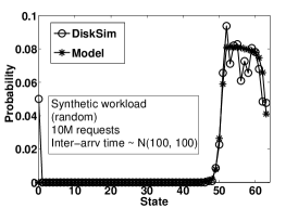
(d) Random + non-Poisson

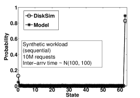
(e) Sequential + non-Poisson

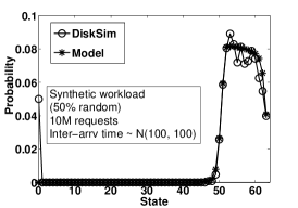
(f) Hybrid + non-Poisson

Figure 2: Model validation on the system state $\boldsymbol{\pi}$. In each sub-figure, the x-axis represents the states (i.e., the number of valid pages in a block), and the y-axis indicates the state probabilities.

Figure 2 show the simulation and model results for the Random, Sequential, and Hybrid workloads, each associated with either the Poisson or non-Poisson arrivals of requests. The results show that under different synthetic workloads, our model derived from the mean field technique can still provide good approximations of the system state compared with that obtained from the simulations. Note that we also observe good approximations even for non-Poisson arrivals of requests. The results show the robustness of our model in evaluating the system state.

5.2 Validation on Operational Points of RGA

In §3, we characterize the optimal tradeoff curve between cleaning cost and wear-leveling; in §4, we present a GC algorithm called RGA that can be tuned by a parameter $d$ to adjust the tradeoff between cleaning cost and wear-leveling. We now validate that RGA can indeed be tuned to operate on the optimal tradeoff curve.

We consider different system state distributions $\boldsymbol{\pi}$ to study the performance of RGA. We first consider $\boldsymbol{\pi}$ derived for the uniform workload (i.e., Equation (6)). We also consider three different distributions of $\boldsymbol{\pi}$ that are drawn from truncated normal distributions, denoted by $N(\mu,\sigma^{2})$ with mean $\mu$ and standard deviation $\sigma$. Figure 3(a) illustrates the four system state distributions, where the mean and variance of each truncated normal distribution are shown in the figure.

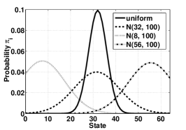
(a) Distributions of $\boldsymbol{\pi}$

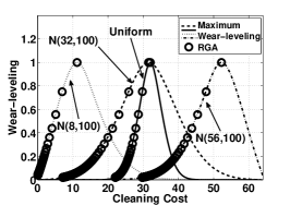
(b) Design space and performance of RGA
for different integers of $d$ from 1 to 100

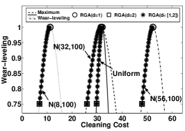
(c) Design space and performance of RGA for different non-integers of $d$ from 1 to 2

Figure 3: Full design space and the performance of RGA.

For each system state distribution, we compute the maximum wear-leveling $\mathcal{W^{*}}$ for each cleaning cost $\mathcal{C^{*}}$ based on Theorem 3. Also, we evaluate the performance of RGA by varying the window size $d$ from 1 to 100, and obtain the corresponding cleaning cost and wear-leveling based on Equations (18) and (19). Here, we only focus on the integer values of $d$.

Figure 3(b) shows the results, in which the four curves represent the optimal tradeoff curves corresponding to the four different distributions of $\boldsymbol{\pi}$, while the circles correspond to the operational points of RGA with different integer values of window size $d$ from 1 to 100. Note that the maximum wear-leveling corresponds to RGA with window size $d=1$ (i.e., the random algorithm). As the window size increases, the wear-leveling decreases, while the cleaning cost also decreases. We observe that RGA indeed operates along the optimal tradeoff curves with regard to different system state distributions.

It is important to note that we can realize non-integer window sizes to further fine-tune RGA along the optimal tradeoff curve (see §4.3). To validate, we consider different values of $d$ from 1 to 2, with step size 0.05, and calculate $d$ via linear extrapolation between 1 and 2.

Figure 3(c) shows the results for non-integer $d$ using different system state distributions. Here, we zoom into the wear-leveling values from 0.75 to 1. Each star corresponds to the RGA with a non-integer window size obtained by Equation (20). We observe that RGA can be further fine-tuned to operate along the optimal tradeoff curves even when $d$ is a non-integer.

6 Trace-Driven Evaluation

In this section, we evaluate the performance of RGA under more realistic settings. Since today’s SSD controllers are mainly proprietary firmware, it is non-trivial to implement GC algorithms inside a real-world SSD controller. Thus, similar to §5, we conduct our evaluation using the DiskSim simulator [8] with SSD extensions [1]. This time we focus on a large-scale SSD. We consider several real-world traces, and evaluate different metrics, including cleaning cost, I/O throughput, wear-leveling, and durability, for different GC algorithms. Note that the cleaning cost and wear-leveling are the metrics considered in the model, while the I/O throughput and durability are the metrics related to user experience.

Using trace-driven evaluation, our goal is to demonstrate the effectiveness of RGA in practical deployment. We compare different variants of RGA with regard to different values of window size $d$, as well as the random and greedy algorithms. We emphasize that we are not advocating a particular value of $d$ for RGA in real deployment; instead, we show how different values of $d$ can be tuned along the performance-durability tradeoff.

6.1 Datasets

We first describe the datasets that drive our evaluation. Since the read requests do not influence our analysis, we focus on four real-world traces that are all write-intensive:

Trace	Total # of requests	Write ratio	Sequential ratio	Avg. request size	Avg. inter-arrival time
Financial	4.4 M	0.7782	0.0167	5.4819 KB	9.9886 ms
Webmail	7.8 M	0.8186	0.7868	4 KB	222.118 ms
Online	5.7 M	0.7388	0.7373	4 KB	303.763 ms
Webmail+Online	13.5 M	0.7849	0.7597	4 KB	128.302 ms

Table 1: Workload statistics of traces.

• Financial [43]: It is an I/O trace collected from an online transaction process application running at a large financial institution. There are two financial traces in [43], namely Financial1.spc and Financial2.spc. Since Financial2.spc is read-dominant, we only use Financial1.spc in this paper.

• Webmail [45]: It is an I/O trace that describes the webmail workload of a university department mail server.

• Online [45]: It is an I/O trace that describes the coursework management workload on Moodle at a university.

• Webmail+Online [45]: It is the combination of the I/O traces of Webmail and Online.

Table 1 summarizes the statistics of the traces. The original Financial trace in [43] contains 24 application-specific units (ASUs) of a storage server (denoted by ASU0 to ASU23). We study the traces of all ASUs except ASU1, ASU3, and ASU5, whose maximum logical sector numbers go beyond the logical address space in our configured SSD (see §6.2). The remaining Financial trace contains around 4.4 million I/O requests, in which 77.82% are write requests and the remaining are read requests. Also, 1.67% of I/O requests are sequential requests, each of which has its starting address immediately following the last address of its prior request. The average size of each request is 5.4819KB, meaning that most requests only access one page as the size of one page is configured as 4KB in the simulation. The average inter-arrival time of two continuous requests is just around 10 ms. On the other hand, for the Webmail, Online and Webmail+Online traces obtained from [45], the write requests account for around 80% of I/O requests, and over 70% of I/O requests are sequential requests. Moreover, all requests in those traces have size 4KB (i.e., only one page is accessed in each request), and the average inter-arrival time is much longer than that of the Financial trace. In summary, the Financial trace has the random-write-dominant access pattern, while the Webmail, Online, and Webmail+Online traces have the sequential-write-dominant access pattern.

We set the page size of an SSD as 4KB (the default value in most today’s SSDs). Since the block size considered by these traces is 512 bytes, we align the I/O requests of these traces to be multiples of the 4KB page size. To enable us to evaluate different GC algorithms, we need to make the blocks in an SSD undergo a sufficient number of program-erase cycles. However, these traces may not be long enough to trigger enough block erasures. Thus, we propose to replay a trace; that is, in each replay cycle, we make a copy of the original trace without changing its I/O patterns, while we only change the arrival times of the requests by adding a constant value. In our simulations, we replay the traces multiple times so that each trace file contains around 50M I/O requests. Since we replay a trace, we issue the same write request to a page multiple times, and this keeps invalidating pages due to out-of-place writes. Thus, many GC operations will be triggered, and this enables us to stress-test the cleaning cost and wear-leveling metrics. We point out that this replay approach has also been used in the prior SSD work [38].

6.2 System Configuration

Table 2 summarizes the parameters that we use to configure an SSD in our evaluation. We use the default configurations from the simulator whose parameters are based on a common SLC SSD [13]. Specifically, the SSD contains 8 flash packages, each of which has its own control bus and data bus, so they can process I/O requests in parallel. Each flash package contains 8 planes containing 2048 blocks each. Each block contains 64 pages of size 4KB each. Therefore, each flash package contains 16384 physical blocks in total and the physical capacity of the SSD is 32GB. For the timing parameters, the time to read one page from the flash media to the register in the plane is 25$\mu$s, and the time of programming one page from the register in the plane to the flash media is 0.2ms. For an erase operation, it takes 1.5ms to erase one block. The time of transferring one byte through the data bus line is 0.025$\mu$s. Since an SSD is usually over-provisioned, we set the over-provisioning factor as 15%, which means that the advertised capacity of an SSD is only 85% of the physical capacity. Moreover, we set the threshold of triggering GC as 5%, meaning that GC will be triggered when the number of free blocks in the system is smaller than 5%. Since flash packages are independent in processing I/O requests, GC is also triggered independently in each flash package. In the following, we only focus on a single flash package and compare the performance of different GC algorithms.

We consider two different initial states of an SSD before we start our simulations. The first one is the empty state, meaning that the SSD is entirely clean and no data has been stored. The second one is the full state, meaning the SSD is fully occupied with valid data and each logical address is always mapped to a physical page containing valid data. Thus, each write request to a (valid) page will trigger an update operation, which writes the new data to a clean page and invalidates the original page. Note that the full initial state is the default setting in the simulator. In most of our simulations (§6.3-§6.5), we use the full initial state as it can be viewed as “stress-testing” the I/O performance of an SSD. When we study the durability of SSDs (§6.6), we use the empty initial state as it can be viewed as the state of a brand-new SSD.

Parameter	Value
page size	4KB
# of pages per block	64
# of blocks per package	16384
# of packages per SSD	8
SSD capacity	32 GB
read one page	0.025ms
write one page	0.2ms
erase one block	1.5ms
transfer one byte	0.000025ms
over-provisioning	15%
threshold of triggering GC	5%

Table 2: Configuration parameters.

6.3 Cleaning Cost

We first evaluate the cleaning cost of different GC algorithms. In particular, we execute the traces with each of the GC algorithms and record the total number of GC operations and the total number of valid pages which are written back due to GC. We then derive the cleaning cost as the average number of valid pages that are written back in each GC operation.

Figure 4 shows the simulation results. In this figure, there are four groups of bars which correspond to the Financial, Webmail, Online, and Webmail+Online traces, respectively. In each group, there are seven bars which correspond to the greedy algorithm, random algorithm and RGA with different window sizes $d$. The vertical axis represents the cleaning cost that each GC algorithm incurs. In this simulation, the simulator starts from the full initial state. We can see that the greedy algorithm incurs the smallest cleaning cost that is almost 0, while the random algorithm has the highest cleaning cost that is close to the total number of pages in each block (i.e., $k$=64). The intuition is that if the greedy algorithm is used, then for every GC operation, the block containing the smallest number of valid pages is reclaimed, which means that it only needs to read out and write back the smallest number of pages. Therefore, the cleaning cost of the greedy algorithm should be the smallest among all algorithms. Moreover, RGA provides a variable cleaning cost between the greedy and random algorithms.

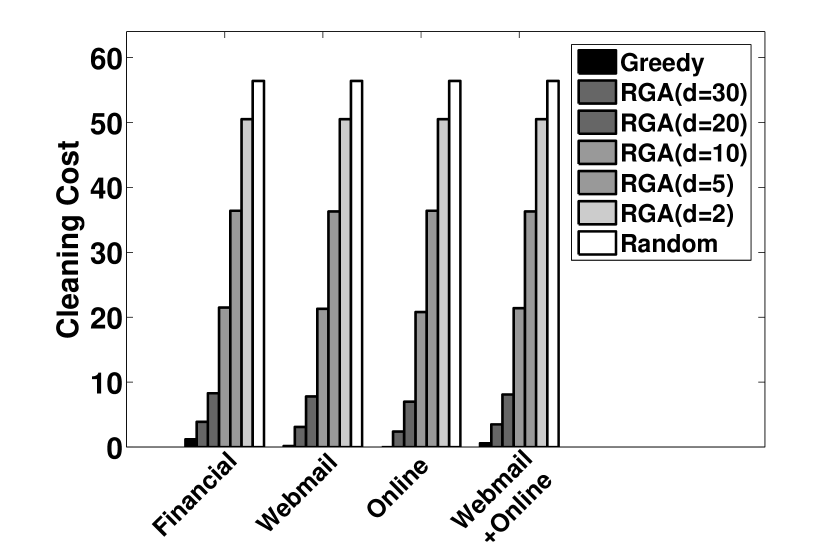
Figure 4: Cleaning cost of different GC algorithms.

6.4 Impact on I/O Throughput

We now consider the impact of different GC algorithms on the I/O throughput, using the metric Input/Output Operations Per Second (IOPS). Note that IOPS is an indirect indicator of the cleaning cost. Specifically, the higher the cleaning cost, the more pages needed to be moved in each GC operation. This prolongs the duration of a GC operation, and leads to smaller IOPS as an I/O request must be queued for a longer time until a GC operation is finished.

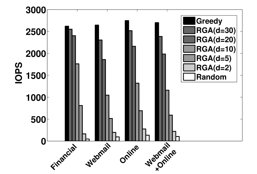
Figure 5: IOPS of different GC algorithms.

Figure 5 shows the IOPS results of different GC algorithms (note that the simulator starts from the full initial state). We can see that the greedy algorithm achieves the highest IOPS, and the random algorithm has the lowest IOPS, which is less than 5% of the IOPS achieved by the greedy algorithm. The results conform to those in Figure 4. This means that the cleaning cost, the metric that we use in our analytical model, correctly reflects the resulting I/O performance. Again, RGA can provide different I/O throughput results with different values of $d$.

6.5 Wear-Leveling

We now evaluate the wear-leveling of different GC algorithms. In the simulation, we execute the traces with each of the GC algorithms and record the number of times that each block has been erased. We then estimate the probability that each block is chosen for GC and derive the wear-leveling based on its definition in Equation (12).

Figure 6 shows the wear-leveling results. It is clear that the random algorithm always achieves the maximum wear-leveling, which is almost one. This implies that the random algorithm can effectively balance the numbers of erasures across all blocks. On the other hand, the greedy algorithm achieves the minimum wear-leveling which is less than 0.2 for all traces. Here, we note that in all traces, our RGA realizes different levels of wear-leveling between the random and greedy algorithms with different values of $d$. In particular, when $d\leq 2$, the wear-leveling of RGA is within 80% of the maximum wear-leveling of the random algorithm.

Figure 6: Wear-leveling of different GC algorithms.

6.6 Impact on Durability

The previous wear-leveling experiment provides insights into the durability (or lifetime) of an SSD. In this evaluation, we focus on examining how the durability of an SSD is affected by different GC algorithms.

To study the durability of an SSD, we have to make the SSD continue handling a sufficient number of I/O requests until it is worn out. In order to speed up our simulation, we decrease the maximum number of erasures sustainable by each block to 50. We also reduce the size of the SSD such that each flash package contains 4096 blocks, so the size of each flash package is 1GB. Other configurations are the same as we described in §6.2. Also, instead of using the real-world traces as in previous simulations, we drive the simulation with the synthetic traces that have more aggressive I/O rates so that the SSD is worn out soon. Specifically, we consider the same set of synthetic traces Random, Hybrid and Sequential as described in §5.1, but here we set the mean inter-arrival time of I/O requests to be 10ms (as opposed to 100ms in §5.1) based on Poisson arrivals.

Due to the use of bad block management [36], an SSD can allow a small percentage of bad (worn-out) blocks during its lifetime. Suppose that the SSD can allow up to $e$% of bad blocks for some parameter $e$. To derive the durability of the SSD, we first continue running each workload trace on the SSD until $e$% blocks are worn out, i.e., the erasure limit is reached. Then we record the length of the duration span that the SSD survives, and take it as the durability of the SSD. For comparison, we normalize the durability with respect to that of the greedy algorithm (which is expected to have the minimum durability). In this experiment, we consider the case where $e$% = 5%, while we also verify that similar observations are made for other values of $e\%\leq 10\%$. Also, we assume that the SSD is brand-new (i.e., the initial state is empty) and all blocks have no erasure at the beginning.

Figure 7 shows the results. We observe that the durability results of different GC algorithms are consistent with those of wear-leveling in Figure 6. We observe that the random algorithm achieves the maximum durability, and the value can be almost six times over that of the greedy algorithm (e.g., in the Sequential workload). Again, RGA provides a tunable durability between the random and greedy algorithms. When the window size $d\leq 5$, the durability of RGA can be within 68% of the maximum lifetime of the random algorithm for Random and Hybrid workloads. For the Sequential workload, the durability of RGA drops to 40% of the maximum lifetime of the random algorithm when $d=5$. However, it is still almost 3 times higher than that of the greedy algorithm.

Figure 7: Durability of different GC algorithms (normalized with respect to the greedy algorithm).

6.7 Summary

From the above simulations, we see that the greedy algorithm performs the best and the random algorithm performs the worst in terms of cleaning cost and I/O throughput, while the opposite holds in terms of wear-leveling and durability. We demonstrate that our RGA provides a tradeoff spectrum between the two algorithms by tuning the window size. This simulation study not only confirms our theoretical model, but also shows that our RGA can be viewed as an effective tunable algorithm to balance between throughput performance and durability of an SSD.

7 Related Work

The research on NAND-flash based SSDs has recently received a lot of attention. Many aspects of SSDs are being studied. A survey on algorithms and data structures for flash memories can be found in [22]. Kawaguchi et al. [31] propose a flash-based file system based on the log-structured file system design. Birrell et al. [6] propose new data structures to improve the write performance of SSDs, and Gupta et al. [25] suggest to exploit value locality and design content addressable SSDs so as to optimize the performance. Matthews et al. [35] use NAND-based disk caching to mitigate the I/O bottlenecks of HDDs, and Kim et al. [32] consider hybrid storage by combining SSDs and HDDs. Agrawal et al. [1] study different design tradeoffs of SSDs via a trace-driven simulator based on DiskSim [8]. Chen et al. [13] further reveal many intrinsic characteristics of SSDs via empirical measurements. Polte et al. [41] also study the performance of SSDs via experiments, and Park et al. [40] mainly focus on the energy efficiency of SSDs. Note that [1] addresses the tradeoff between cleaning cost and wear-leveling in GC, but it is mainly based on empirical evaluation.

A variety of wear-leveling techniques have been proposed, mainly from an applied perspective. Some of them are proposed in patents [2, 7, 20, 26, 34, 46, 3]. Several research papers have been proposed to maximize wear-leveling in SSDs based on hot-cold swapping, whose main idea is to swap the frequently-used hot data in worn blocks and the rarely-used cold data in new blocks. For example, Chiang et al. [15, 14] propose clustering methods for hot/cold data based on access patterns to maximize wear-leveling. Jung et al. [30] propose a memory-efficient design for wear-leveling by tracking only block groups, while maintaining wear-leveling performance. Authors of [10, 12, 11] also propose different strategies based on hot-cold swapping to further improve the wear-leveling performance. Our work differs from above studies in that we focus on characterizing the optimal tradeoff of GC algorithms, such that we provide flexibility for SSD practitioners to reduce wear-leveling to trade for higher cleaning performance. We also propose a tunable GC algorithm to realize the tradeoff.

From a theoretical perspective, some studies propose analytical frameworks to quantify the performance of GC algorithms. A comparative study between online and offline wear-leveling policies is presented in [4]. Hu et al. [28] propose a probabilistic model to quantify the additional writes due to GC (i.e., the cleaning cost defined in our work). They study a modified greedy GC algorithm, and implement an event-driven simulator to validate their model. Bux and Iliadis [9] propose theoretical models to analyze the greedy GC algorithm under the uniform workload, and Desnoyers [18] also analyzes the performance of LRU and greedy GC algorithms when page-level address mapping is used. Our work differs from them in the following. First, the previous work focuses on analyzing the write amplification which corresponds to the cleaning cost in our paper, but our focus is to analyze the tradeoff between cleaning cost and wear-leveling, which are both very important in designing GC algorithms, and further explore the design space of GC algorithms. Second, our analytical models are also very different. In particular, we use a Markov model to characterize the I/O dynamics of SSDs and adapt the mean field technique to approximate large-scale systems, then we develop an optimization framework to derive the optimal tradeoff curve. Finally, our model also provides a good approximation under general workload and address mapping, and it is further validated via trace-driven evaluation.

We note that an independent analytical work [44], which is published in the same conference as ours, also applies the mean-field technique to analyze different GC algorithms. Its $d$-choices GC algorithm has the same construction as our RGA. Our work has the following key differences. First, similar to prior analytical studies, the work [44] focuses on write amplification, while we focus on the trade-off between cleaning cost and wear leveling. Second, its analysis is limited to the uniform workload only, while we also address the general workload. Finally, we validate our analysis via trace-driven simulations, which are not considered in the work [44].

8 Conclusions

In this paper, we propose an analytical model to characterize the performance-durability tradeoff of an SSD. We model the I/O dynamics of a large-scale SSD, and use the mean field theory to derive the asymptotic results in equilibrium. In particular, we classify the blocks of an SSD into different types according to the number of valid pages contained in each block, and our mean field results can provide effective approximation on the fraction of different types of blocks in the steady state even under the general workload. We define two metrics, namely cleaning cost and wear-leveling, to quantify the performance of GC algorithms. In particular, we theoretically characterize the optimal tradeoff curve between cleaning cost and wear-leveling, and develop an optimization framework to explore the full optimal design space of GC algorithms. Inspired from our analytical framework, we develop a tunable GC algorithm called the randomized greedy algorithm (RGA) which can efficiently balance the tradeoff between cleaning cost and wear-leveling by tuning the parameter of the window size $d$. We use trace-driven simulation based on DiskSim with SSD add-ons to validate our analytical model, and show the effectiveness of RGA in tuning the performance-durability tradeoff in deployment.

Appendix A Proof of Convergence

We now formally prove the convergence of the SSD system state under the uniform workload. Our proof consists of two parts. We first prove that the stochastic process $\boldsymbol{M}^{N}(t)$ indeed converges to the deterministic process $\boldsymbol{s}(t)$ when $N\rightarrow\infty$. We then prove that the deterministic process described in Equation (5) converges to the unique fixed point $\boldsymbol{\pi}$ in Equation (6).

We first show that the re-scaled process $\widetilde{\boldsymbol{M}}^{N}(t)$ converges to $\boldsymbol{s}(t)$. Let us first show several important properties of the stochastic process $\boldsymbol{M}^{N}(t)$.

Lemma 1

Define $S=\{\boldsymbol{m}\!\in\!R^{k+1}|\sum_{i=0}^{k}m_{i}\!=\!1,m_{i}\geq 0\,\forall i\}$. For any $\boldsymbol{s}\in S$, let $\boldsymbol{f}^{N}(\boldsymbol{s})=E(\boldsymbol{M}^{N}(t+1)-\boldsymbol{M}^{N}(t)|\boldsymbol{M}^{N}(t)=\boldsymbol{s})$ be the expected change to the occupancy measure in one time slot, and let $\varepsilon(N)=1/N$. We have $\lim_{N\rightarrow\infty}\varepsilon(N)$$=0$, and $\lim_{N\rightarrow\infty}\frac{\boldsymbol{f}^{N}(\boldsymbol{s})}{\varepsilon(N)}$ exists for $\forall\boldsymbol{s}\in S$.

Proof: Since $\varepsilon(N)=\frac{1}{N}$, $\lim_{N\rightarrow\infty}\varepsilon(N)=0$. Denote $\boldsymbol{f}^{N}(\boldsymbol{s})=(f^{N}_{0}(\boldsymbol{s}),f^{N}_{1}(\boldsymbol{s}),...,f^{N}_{k}(\boldsymbol{s}))$. Consider the expected change in $M_{i}(t)$ ($1\leq i\leq k-1$) during one time slot when $\lambda$ requests arrive. For each request, the probability of changing a block of type $i$ to other states is $\frac{1}{N}Ns_{i}$, and the corresponding change in $M_{i}(t)$ is $-\frac{1}{N}$. A request may also change blocks of type $i+1$ (or type $i-1$) to state $i$, with probability being $\frac{i+1}{Nk}Ns_{i+1}$ (or $\frac{k-i+1}{Nk}Ns_{i-1}$) and the change in $M_{i}(t)$ being $\frac{1}{N}$ (or $\frac{1}{N}$). Thus, we have

$$f^{N}_{i}(\boldsymbol{s})\!=\!-\frac{1}{N}\lambda s_{i}+\frac{i+1}{Nk}\lambda s_{i+1}+\frac{k-i+1}{Nk}\lambda s_{i-1},1\!\leq\!i\!\leq k\!-\!1.$$

Similarly, we can also derive $f^{N}_{0}(\boldsymbol{s})$ and $f^{N}_{k}(\boldsymbol{s})$. Therefore, we have $\lim_{N\rightarrow\infty}\frac{\boldsymbol{f}^{N}(\boldsymbol{s})}{\varepsilon(N)}=\boldsymbol{f}(\boldsymbol{s})$, where

$$\left\{\begin{aligned} f_{i}(\boldsymbol{s})=&-\lambda s_{i}\!+\!\frac{i+1}{k}\lambda s_{i+1}\!+\!\frac{k-i+1}{k}\lambda s_{i-1},\quad 1\!\leq\!i\!\leq\!k\!-\!1,\\ f_{0}(\boldsymbol{s})=&-\lambda s_{0}+\frac{1}{k}\lambda s_{1};\,\,\,f_{k}(\boldsymbol{s})=-\lambda s_{k}+\,\frac{1}{k}\lambda s_{k-1}.\hskip 28.0pt\rule{5.12149pt}{7.11317pt}\end{aligned}\right.$$

Lemma 2

Define $W^{N}(t)$ as an upper bound on the number of blocks that make a transition in time slot $t$. Then $W^{N}(t)$ satisfies $E(W^{N}(t)^{2}|\boldsymbol{M}^{N}(t)=\boldsymbol{s})\leq cN^{2}\varepsilon(N)^{2}$ where $c$ is a constant.

Proof: During the time slot $t$, $\lambda$ requests arrive, and for each request, it accesses a block with probability $\frac{1}{N}$. Therefore, $W^{N}(t)$ follows a binomial distribution with parameters $\frac{\lambda}{N}$ and $N$.

$$E(W^{N}(t)^{2}|\boldsymbol{M}^{N}(t)\!=\!\boldsymbol{s})\!=\!\left(\!N\frac{\lambda}{N}\!\right)^{2}\!+\!N\frac{\lambda}{N}\left(\!1\!-\!\frac{\lambda}{N}\!\right)\leq\lambda^{2}\!+\!\lambda,$$

which shows the result in Lemma 2 with $c=\lambda^{2}+\lambda$.  

Lemma 3

There exists $\beta>0$ and a function $\varphi(\boldsymbol{s},\alpha)$ defined on $S\times[0,\beta]$ such that $\varphi$ has continuous derivatives everywhere and $\frac{\boldsymbol{f}^{N}(\boldsymbol{s})}{\varepsilon(N)}=\varphi(\boldsymbol{s},\frac{1}{N})$.

Proof: From the proof of Lemma 1, $\frac{\boldsymbol{f}^{N}(\boldsymbol{s})}{\varepsilon(N)}=\boldsymbol{f}(\boldsymbol{s})$. Since $\boldsymbol{f}(\boldsymbol{s})$ is a rational function with respect to $\boldsymbol{s}$ and $\frac{1}{N}$, Lemma 3 holds.  

Now, we can now show that the re-scaled process $\widetilde{\boldsymbol{M}}^{N}(t)$ converges to $\boldsymbol{s}(t)$, with the following theorem.

Theorem 4

If $\boldsymbol{M}^{N}(0)\rightarrow\boldsymbol{m}$ in probability as $N\rightarrow\infty$, then for all $T>0$, $\sup_{0\leq t\leq T}\|\widetilde{\boldsymbol{M}}^{N}(t)-\boldsymbol{s}(t)\|\rightarrow 0$ in probability, where $\boldsymbol{s}(t)$ satisfies the ODEs in Equation (5) and $\boldsymbol{s}(0)=\boldsymbol{m}$.

Proof: The theorem holds due to Lemmas 1, 2, and 3, and the existing theorem in [5] (Corollary 1).  

Note that the theorem in [5] provides a way to prove the convergence to mean field limit, provided that several sufficient conditions hold. Therefore, to invoke the theorem in [5], we must explicitly verify that our model indeed satisfies the conditions, i.e., Lemma 1-3, so as to make the proof complete.

Corollary 1

If $\boldsymbol{M}^{N}(0)\rightarrow\boldsymbol{m}$ in probability as $N\rightarrow\infty$, then for all $T>0$, $\sup_{0\leq t\leq T}\|\boldsymbol{M}^{N}(t)-\boldsymbol{s}(\frac{t}{N})\|\rightarrow 0$ in probability, where $\boldsymbol{s}(t)$ satisfies the ODEs in Equation (5) and $\boldsymbol{s}(0)=\boldsymbol{m}$.

In the following, we prove that the deterministic process $\boldsymbol{s}(t)$ in Equation (5) converges to the unique fixed point $\boldsymbol{\pi}$ in Equation (6). Note that the ODEs in Equation (5) is just a special case of the ODEs in Equation (8). Since our proof also applies to the general case, to avoid redundancy, we directly present the convergence proof of the general case, i.e., the convergence of the ODEs in Equation (8) to the fixed point in Equation (9). The detailed proof is shown in Theorem 5. We thank professor Benny Van Houdt for giving us invaluable comments on this proof.

Theorem 5

The deterministic process $\boldsymbol{s}(t)$ which is specified by ODEs (8) converges to the fixed point $\boldsymbol{\pi}$ which is determined by Equation (9).

Proof: Note that Equation (8) can be rewritten as follows.

$$\frac{d\mbox{\boldmath$s$}(t)}{dt}=\mbox{\boldmath$s$}(t)\mbox{\boldmath$Q$},$$ (21)

where $\mbox{\boldmath$s$}(t)=(s_{0}(t),s_{1}(t),...,s_{k}(t))$ and $\mbox{\boldmath$Q$}=[q_{i,j}]$.

$$q_{i,j}=\left\{\begin{aligned} &\lambda p_{i,j},&\mbox{for}j\neq i,\\ &-\lambda p_{0,1},&\mbox{ for }j=i=0,\\ &-\lambda p_{k,k-1},&\mbox{ for }j=i=k,\\ &-\lambda(p_{i,i-1}+p_{i,i+1}),&\mbox{ for }0<j=i<k.\end{aligned}\right.$$

Note that if we treat the state transition of a particular block shown in Figure 1 as a birth-death process, then Equation (21) exactly maps to the Kolmogorov’s forward equations where $Q$ is just the rate matrix of the birth-death process. Therefore, $\mbox{\boldmath$s$}(t)$ converges to the stationary distribution of the birth-death process $\boldmath{\pi}$ where $\boldmath{\pi}\mbox{\boldmath$Q$}=\boldmath{0}$. We can easily verity that the fixed point $\boldmath{\pi}$ in Equation (9) satisfies the condition $\boldmath{\pi}\mbox{\boldmath$Q$}=\boldmath{0}$, which completes the proof.  

Note that Theorem 5 also completes the proof that the ODEs in Equation (5) converges to the unique fixed point $\boldsymbol{\pi}$ in Equation (6).

Appendix B Proof of Optimal Design Space

We now prove Theorem 3 in §3.4. We solve Equation (3.4) by minimizing the inverse of the objective function, and the problem is a convex optimization problem. If a point $(\boldsymbol{\tilde{w}},\boldsymbol{\tilde{u}},\tilde{v_{1}},\tilde{v_{2}})$ satisfies the KKT conditions which are stated in Equation (22), then $\boldsymbol{\tilde{w}}$ is the global minimum.

$$\left\{\begin{aligned} &2w_{i}\pi_{i}-u_{i}+v_{1}\pi_{i}+v_{2}i\pi_{i}=0;\,\,\,u_{i}\geq 0;\,\,\,w_{i}\geq 0;\\ &u_{i}w_{i}=0;\,\,\,\sum\nolimits_{i=0}^{k}w_{i}\pi_{i}=1;\,\,\,\sum\nolimits_{i=0}^{k}iw_{i}\pi_{i}=\mathcal{C^{*}}.\end{aligned}\right.$$ (22)

To find a point satisfying the KKT conditions, we first consider the case when $0<\mathcal{C^{*}}<\sum_{i=0}^{k}i\pi_{i}$. Let

$${\cal I}_{1}=\min_{0\leq j\leq k}\{j:\sum\nolimits_{i=0}^{j}i\pi_{i}\!-\!\mathcal{C^{*}}\sum\nolimits_{i=0}^{j}\pi_{i}>0\}.$$ (23)

Note that ${\cal I}_{1}$ must exist because $\mathcal{C^{*}}\!<\!\sum_{i=0}^{k}i\pi_{i}$ and $\sum_{i=0}^{k}\pi_{i}\!=\!1$. Clearly, we have ${\cal I}_{1}>\mathcal{C^{*}}$ and $\sum_{i=0}^{j}i\pi_{i}\!-\!\mathcal{C^{*}}\sum_{i=0}^{j}\pi_{i}>0\,\mbox{ for }{\cal I}_{1}\leq j\leq k.$ Moreover, we have $\sum_{i=0}^{j}i^{2}\pi_{i}-\mathcal{C^{*}}\sum_{i=0}^{j}i\pi_{i}>0$ (${\cal I}_{1}\leq j\leq k$). Now we prove that the following inequality holds.

$$\frac{\sum_{i=0}^{{\cal I}_{1}}i^{2}\pi_{i}-\mathcal{C^{*}}\sum_{i=0}^{{\cal I}_{1}}i\pi_{i}}{\sum_{i=0}^{{\cal I}_{1}}i\pi_{i}-\mathcal{C^{*}}\sum_{i=0}^{{\cal I}_{1}}\pi_{i}}>{\cal I}_{1}.$$ (24)

To prove the inequality (24), we rewrite the left hand side of the inequality as follows.

$$\frac{\sum_{i=0}^{{\cal I}_{1}}i^{2}\pi_{i}-\mathcal{C^{*}}\sum_{i=0}^{{\cal I}_{1}}i\pi_{i}}{\sum_{i=0}^{{\cal I}_{1}}i\pi_{i}-\mathcal{C^{*}}\sum_{i=0}^{{\cal I}_{1}}\pi_{i}}\triangleq \frac{-ax+by+{\cal I}_{1}z}{-x+y+z},$$

where $x=-\sum_{i=0}^{\lfloor\mathcal{C^{*}}\rfloor}(i-\mathcal{C^{*}})\pi_{i}$, $y=\sum_{i=\lfloor\mathcal{C^{*}}\rfloor+1}^{{\cal I}_{1}-1}(i-\mathcal{C^{*}})\pi_{i}$ and $z=({\cal I}_{1}-\mathcal{C^{*}})\pi_{{\cal I}_{1}}$. Clearly, we have $x>0,y\geq 0,z>0$ and ${\cal I}_{1}>b>a>0$. Since ${\cal I}_{1}$ is the smallest integer which satisfies the condition in (23), we also have $-x+y<0$ and $-x+y+z>0$. Now, if $-ax+by\geq 0$, then inequality (24) holds. Otherwise,

$$\frac{-ax+by+{\cal I}_{1}z}{-x+y+z}={\cal I}_{1}+\frac{({\cal I}_{1}-a)(x-y)+(b-a)y}{-x+y+z}$$

$$> {\cal I}_{1}(\mbox{ as }{\cal I}_{1}>b>a>0,-x+y<0,\mbox{ and }-x+y+z>0).$$

Now, we argue that there exists an ${\cal I}$ (${\cal I}_{1}\leq{\cal I}\leq k$) such that

$$\left\{\begin{aligned} &{\cal I}\!<\!k\mbox{ and }{\cal I}\!<\!\frac{\sum_{i=0}^{{\cal I}}i^{2}\pi_{i}-\mathcal{C^{*}}\sum_{i=0}^{{\cal I}}i\pi_{i}}{\sum_{i=0}^{{\cal I}}i\pi_{i}-\mathcal{C^{*}}\sum_{i=0}^{{\cal I}}\pi_{i}}\!\leq\!{\cal I}+1,\mbox{ or }\\ &{\cal I}\!=\!k\mbox{ and }{\cal I}\!<\!\frac{\sum_{i=0}^{{\cal I}}i^{2}\pi_{i}-\mathcal{C^{*}}\sum_{i=0}^{{\cal I}}i\pi_{i}}{\sum_{i=0}^{{\cal I}}i\pi_{i}-\mathcal{C^{*}}\sum_{i=0}^{{\cal I}}\pi_{i}}.\end{aligned}\right.$$ (25)

To prove it, we can examine from ${\cal I}_{1}$. Since inequality (24) holds, if ${\cal I}_{1}<k$ and $\frac{\sum_{i=0}^{{\cal I}_{1}}i^{2}\pi_{i}-\mathcal{C^{*}}\sum_{i=0}^{{\cal I}_{1}}i\pi_{i}}{\sum_{i=0}^{{\cal I}_{1}}i\pi_{i}-\mathcal{C^{*}}\sum_{i=0}^{{\cal I}_{1}}\pi_{i}}>{\cal I}_{1}+1$, then we have

$$\frac{\sum_{i=0}^{{\cal I}_{1}+1}i^{2}\pi_{i}-\mathcal{C^{*}}\sum_{i=0}^{{\cal I}_{1}+1}i\pi_{i}}{\sum_{i=0}^{{\cal I}_{1}+1}i\pi_{i}-\mathcal{C^{*}}\sum_{i=0}^{{\cal I}_{1}+1}\pi_{i}}>{\cal I}_{1}+1.$$

Therefore, either we find an ${\cal I}$ such that ${\cal I}\!\!<\!\!\frac{\sum_{i=0}^{{\cal I}}\!i^{2}\pi_{i}-\mathcal{C^{*}}\sum_{i=0}^{{\cal I}}\!i\pi_{i}}{\sum_{i=0}^{{\cal I}}\!i\pi_{i}-\mathcal{C^{*}}\sum_{i=0}^{{\cal I}}\!\pi_{i}}\!\!\leq\!\!{\cal I}+1$ or we reach $k$. Now, given the ${\cal I}$ in Equation (25), we define

$$\left\{\begin{aligned} X_{{\cal I}}&\!\!=\!\!\sum\nolimits_{i=0}^{\cal I}\!i^{2}\pi_{i}\!-\!\mathcal{C^{*}}\!\sum\nolimits_{i=0}^{\cal I}\!i\pi_{i},\,\,Y_{{\cal I}}\!\!=\!\!\sum\nolimits_{i=0}^{\cal I}\!i\pi_{i}\!-\!\mathcal{C^{*}}\!\sum\nolimits_{i=0}^{\cal I}\!\pi_{i},\\ Z_{{\cal I}}&=\sum\nolimits_{i=0}^{\cal I}\pi_{i}\sum\nolimits_{i=0}^{\cal I}i^{2}\pi_{i}-(\sum\nolimits_{i=0}^{\cal I}i\pi_{i})^{2}.\end{aligned}\right.$$

By Cauchy’s Inequality, we have $Z_{{\cal I}}>0$. If we define

$$\gamma_{i}=X_{{\cal I}}/Z_{{\cal I}}-i\times Y_{{\cal I}}/Z_{{\cal I}},$$ (26)

we have $\gamma_{i}>0,\textrm{ for }0\leq i\leq{\cal I}$, and $\gamma_{i}\leq 0,\textrm{ for }{\cal I}+1\leq i\leq k.$

We can verify that $(\boldsymbol{\tilde{w}},\boldsymbol{\tilde{u}},\tilde{v_{1}},\tilde{v_{2}})$ which is defined as follows satisfies the KKT conditions (22). Thus, $\boldsymbol{\tilde{w}}$ is the global minimum.

$$\left\{\begin{aligned} &\tilde{v}_{1}=-2X_{{\cal I}}/Z_{{\cal I}},\\ &\tilde{v}_{2}=2Y_{{\cal I}}/Z_{{\cal I}},\end{aligned}\right.\,\,\left\{\begin{aligned} &\tilde{w}_{i}=\gamma_{i},\,\,\,\tilde{u}_{i}=0,\,\,0\leq i\leq{\cal I},\\ &\tilde{w}_{i}=0,\,\,\,\tilde{u}_{i}=-2\gamma_{i}\pi_{i},\,\,{\cal I}+1\leq i\leq k,\end{aligned}\right.$$

Similarly, we can find the optimal solution for the case when ${\cal C}^{*}>\sum_{i=0}^{k}i\pi_{i}$. Since the framework of the proof is very similar, we only present the solution. In particular, we define

$$\left\{\!\!\!\begin{aligned} X_{{\cal L}}&\!\!=\!\!\sum\nolimits_{i={\cal L}}^{k}\!i^{2}\pi_{i}\!-\!\mathcal{C^{*}}\!\!\sum\nolimits_{i={\cal L}}^{k}\!i\pi_{i},\,\,Y_{{\cal L}}\!\!=\!\!\sum\nolimits_{i={\cal L}}^{k}\!i\pi_{i}\!-\!\mathcal{C^{*}}\!\!\sum\nolimits_{i={\cal L}}^{k}\!\pi_{i},\\ Z_{{\cal L}}&=\sum\nolimits_{i={\cal L}}^{k}\pi_{i}\sum\nolimits_{i={\cal L}}^{k}i^{2}\pi_{i}-(\sum\nolimits_{i={\cal L}}^{k}i\pi_{i})^{2},\end{aligned}\right.$$

where ${\cal L}$ is an integer which satisfies the following condition.

$${\cal L}\!>\!0\mbox{ and }{\cal L}\!>\!X_{{\cal L}}/Y_{{\cal L}}\!\geq\!{\cal L}-1,\mbox{ or }{\cal L}\!=\!0\mbox{ and }{\cal L}\!>\!X_{{\cal L}}/Y_{{\cal L}}.$$ (27)

If we define

$$\Gamma_{i}=X_{{\cal L}}/Z_{{\cal L}}-i\times Y_{{\cal L}}/Z_{{\cal L}},$$ (28)

we can also verify that $(\boldsymbol{\tilde{w}},\boldsymbol{\tilde{u}},\tilde{v_{1}},\tilde{v_{2}})$ which is defined as follows satisfies the KKT conditions. Therefore, $\boldsymbol{\tilde{w}}$ is the global minimum.

$$\left\{\begin{aligned} &\tilde{v}_{1}=-2X_{{\cal L}}/Z_{{\cal L}},\\ &\tilde{v}_{2}=2Y_{{\cal L}}/Z_{{\cal L}},\end{aligned}\right.\,\,\left\{\begin{aligned} &\tilde{w}_{i}=0,\,\,\,\tilde{u}_{i}=-2\Gamma_{i}\pi_{i},\,\,0\leq i\leq{\cal L}\!-\!1,\\ &\tilde{w}_{i}=\Gamma_{i},\,\,\,\tilde{u}_{i}=0,\,\,{\cal L}\leq i\leq k.\end{aligned}\right.$$

The cases when ${\cal C}^{*}=0$ or $k$ and ${\cal C}^{*}=\sum_{i=0}^{k}i\pi_{i}$ correspond to the greedy and random algorithms, respectively. Therefore, the maximum wear-leveling $\mathcal{W^{*}}$ can be derived as in Equation (16) where $\gamma_{i}$, ${\cal I}$, $\Gamma_{i}$, and ${\cal L}$ are defined by Equations (25)-(28).

References

- [1] N. Agrawal, V. Prabhakaran, T. Wobber, J. D. Davis, M. Manasse, and R. Panigrahy. Design Tradeoffs for SSD Performance. In Proc. of USENIX ATC, Jun 2008.
- [2] M. Assar, S. Nemazie, and P. Estakhri. Flash Memorymass Storage Architecture Incorporation Wear Leveling Technique. US patent 5,479,638, Dec 1995.
- [3] A. Ban. Wear Leveling of Static Areas in Flash Memory. US patent 6732221, May 2004.
- [4] A. Ben-Aroya and S. Toledo. Competitive Analysis of Flash-memory Algorithms. In Proc. of Annual European Symposium, Sep 2006.
- [5] M. Benaïm and J.-Y. L. Boudec. A Class of Mean Field Interaction Models for Computer and Communication Systems. Performance Evaluation, 2008.
- [6] A. Birrell, M. Isard, C. Thacker, and T. Wobber. A Design for High-performance Flash Disks. ACM SIGOPS Oper. Syst. Rev., 41(2):88–93, Apr 2007.
- [7] R. H. Bruce, R. H. Bruce, E. T. Cohen, and A. J. Christie. Unified Re-map and Cache-index Table with Dual Write-counters for Wear-leveling of Non-volitile Flash Ram Mass Storage. US patent 6,000,006, Dec 1999.
- [8] J. S. Bucy, J. Schindler, S. W. Schlosser, and G. R. Ganger. The DiskSim Simulation Environment Version 4.0 Reference Manual. Technical Report CMUPDL-08-101, Carnegie Mellon University, May 2008.
- [9] W. Bux and I. Iliadis. Performance of Greedy Garbage Collection in Flash-based Solid-state Drives. Performance Evaluation, November 2010.
- [10] L.-P. Chang and C.-D. Du. Design and Implementation of an Efficient Wear-leveling Algorithm for Solid-state-disk Microcontrollers. ACM Trans. Des. Autom. Electron. Syst., 15(1):6:1–6:36, Dec 2009.
- [11] L.-P. Chang and L.-C. Huang. A Low-cost Wear-leveling Algorithm for Block-mapping Solid-state Disks. In Proc of SIGPLAN/SIGBED Conf. on LCTES, Apr 2011.
- [12] Y.-H. Chang, J.-W. Hsieh, and T.-W. Kuo. Improving Flash Wear-Leveling by Proactively Moving Static Data. IEEE Tran. on Computers, 59:53–65, Jan 2010.
- [13] F. Chen, D. A. Koufaty, and X. Zhang. Understanding Intrinsic Characteristics and System Implications of Flash Memory Based Solid State Drives. In Proc. of ACM SIGMETRICS, Jun 2009.
- [14] M.-L. Chiang and R.-C. Chang. Cleaning Policies in Mobile Computers Using Flash Memory. J. Syst. Softw., 48(3):213–231, Nov 1999.
- [15] M.-L. Chiang, P. C. H. Lee, and R.-C. Chang. Using Data Clustering to Improve Cleaning Performance for Flash Memory. Softw. Pract. Exper., 29(3):267–290, Mar 1999.
- [16] T.-S. Chung, D.-J. Park, S. Park, D.-H. Lee, S.-W. Lee, and H.-J. Song. System Software For Flash Memory: A Survey. In Proc. of Int. Conf. on Embedded and Ubiquitous Computing, 2006.
- [17] T.-S. Chung, D.-J. Park, S. Park, D.-H. Lee, S.-W. Lee, and H.-J. Song. A Survey of Flash Translation Layer. Journal of Systems Architecture, 55(5-6):332–343, May 2009.
- [18] P. Desnoyers. Analytic Modeling of SSD Write Performance. In Proceedings of SYSTOR, 2012.
- [19] R. Enderle. Revolution in January: EMC Brings Flash Drives into the Data Center. http://www.itbusinessedge.com/blogs/rob/?p=184, Jan 2008.
- [20] P. Estakhri, M. Assar, R. Reid, Alan, and B. Iman. Method of and Architecture for Controlling System Data with Automatic Wear Leveling in a Semiconductor Non-volitile Mass Storage Memory. US patent 5,835,935, Nov 1998.
- [21] D. Floyer. Flash Pricing Trends Disrupt Storage. http://wikibon.org/wiki/v/Flash_Pricing_Trends_Disrupt_Storage, May 2010.
- [22] E. Gal and S. Toledo. Algorithms and Data Structures for Flash Memories. ACM Computing Surveys, 37(2):138–163, Jun 2005.
- [23] L. M. Grupp, J. D. Davis, and S. Swanson. The Bleak Future of NAND Flash Memory. In Proc. of USENIX FAST, 2012.
- [24] A. Gupta, Y. Kim, and B. Urgaonkar. DFTL: A Flash Translation Layer Employing Demand-based Selective Caching of Page-level Address Mappings. In Proc. of ACM ASPLOS, March 2009.
- [25] A. Gupta, R. Pisolkar, B. Urgaonkar, and A. Sivasubramaniam. Leveraging Value Locality in Optimizing NAND Flash-based SSDs. In Proc. of USENIX FAST, 2011.
- [26] S.-W. Han. Flash Memory Wear Leveling System and Method. US patent 6,016,275, Jan 2000.
- [27] K. Hess. 2011: Year of the SSD? http://www.datacenterknowledge.com/archives/2011/02/17/2011-year-of-the-ssd/, Feb 2011.
- [28] X.-Y. Hu, E. Eleftheriou, R. Haas, I. Iliadis, and R. Pletka. Write Amplification Analysis in Flash-based Solid State Drives. In Proc. of SYSTOR, May 2009.
- [29] R. K. Jain, D.-M. W. Chiu, and W. R. Hawe. A Quantitative Measure Of Fairness And Discrimination For Resource Allocation In Shared Computer Systems. Technical report, DEC, 1984.
- [30] D. Jung, Y.-H. Chae, H. Jo, J.-S. Kim, and J. Lee. A Group-based Wear-leveling Algorithm for Large-capacity Flash Memory Storage Systems. In Proc. of Int. Conf. on Compilers, Architecture, and Synthesis for Embedded Systems, Sep 2007.
- [31] A. Kawaguchi, S. Nishioka, and H. Motoda. A Flash-memory Based File System. In Proc. of USENIX Technical Conference, Jan 1995.
- [32] Y. Kim, A. Gupta, B. Urgaonkar, P. Berman, and A. Sivasubramaniam. HybridStore: A Cost-Efficient, High-Performance Storage System Combining SSDs and HDDs. In Proc. of IEEE MASCOTS, Jul 2011.
- [33] S.-W. Lee, D.-J. Park, T.-S. Chung, D.-H. Lee, S. Park, and H.-J. Song. A Log Buffer-based Flash Translation Layer Using Fully-associative Sector Translation. ACM Trans. on Embedded Computing Systems, 6(3), Jul 2007.
- [34] K. M. J. Lofgren, R. D. Norman, G. B. Thelin, and A. Gupta. Wear Leveling Techniques for Flash EEPROM Systems. US patent 6,850,443, Feb 2005.
- [35] J. Matthews, S. Trika, D. Hensgen, R. Coulson, and K. Grimsrud. Intel® Turbo Memory: Nonvolatile Disk Caches in the Storage Hierarchy of Mainstream Computer Systems. ACM Trans. on Storage, 4(2):4:1–4:24, May 2008.
- [36] Micron Technology. Bad Block Management in NAND Flash Memory. Technical Note, TN-29-59, 2011.
- [37] M. Mitzenmacher. Load Balancing and Density Dependent Jump Markov Processes. In Proc. of IEEE FOCS, Oct. 1996.
- [38] M. Murugan and D. Du. Rejuvenator: A Static Wear Leveling Algorithm for NAND Flash Memory with Minimized Overhead. In Proc. of IEEE MSST, May 2011.
- [39] C. Park, W. Cheon, J. Kang, K. Roh, W. Cho, and J.-S. Kim. A Reconfigurable FTL (Flash Translation Layer) Architecture for NAND Flash-based Applications. ACM Trans. Embed. Comput. Syst., 7(4):38:1–38:23, Aug 2008.
- [40] S. Park, Y. Kim, B. Urgaonkar, J. Lee, and E. Seo. A Comprehensive Study of Energy Efficiency and Performance of Flash-based SSD. Journal of Systems Architecture, 57(4):354–365, April 2011.
- [41] M. Polte, J. Simsa, and G. Gibson. Enabling Enterprise Solid State Disks Performance. In 1st Workshop on Integrating Solid-state Memory into the Storage Hierarchy, March 2009.
- [42] Z. Qin, Y. Wang, D. Liu, and Z. Shao. Demand-based Block-level Address Mapping in Large-scale NAND Flash Storage Systems. In Proc. of IEEE/ACM/IFIP CODES+ISSS, Oct 2010.
- [43] Storage Performance Council. http://traces.cs.umass.edu/index.php/Storage/Storage, 2002.
- [44] B. Van Houdt. A Mean Field Model for a Class of Garbage Collection Algorithms in Flash-based Solid State Drives. In Proc. of ACM SIGMETRICS, 2013.
- [45] A. Verma, R. Koller, L. Useche, and R. Rangaswami. SRCMap: Energy Proportional Storage using Dynamic Consolidation. In Proc. of USENIX FAST, Feb 2010. http://sylab.cs.fiu.edu/projects/srcmap/start.
- [46] S. E. Wells. Method for Wear Leveling in a Flash EEPROM Memory. US patent 5,341,339, Aug 1994.