Measuring Protoplanetary Disk Accretion with H I Pfund $\beta$ ¹

Abstract

In this work, we introduce the use of H i Pfund $\beta$ (Pf$\beta$; 4.6538 $\mu$m) as a tracer of mass accretion from protoplanetary disks onto young stars. Pf$\beta$ was serendipitously observed in NIRSPEC and CRIRES surveys of CO fundamental emission, amounting to a sample size of 120 young stars with detected Pf$\beta$ emission. Using a subsample of disks with previously measured accretion luminosities, we show that Pf$\beta$ line luminosity is well correlated with accretion luminosity over a range of at least three orders of magnitude. We use this correlation to derive accretion luminosities for all 120 targets, 65 of which are previously unreported in the literature. The conversion from accretion luminosity to accretion rate is limited by the availability of stellar mass and radius measurements; nevertheless, we also report accretion rates for 67 targets, 16 previously unmeasured. Our large sample size and our ability to probe high extinction values allow for relatively unbiased comparisons between different types of disks. We find that the transitional disks in our sample have lower than average Pf$\beta$ line luminosities, and thus accretion luminosities, at a marginally significant level. We also show that high Pf$\beta$ equivalent width is a signature of transitional disks with high inner disk gas/dust ratios. In contrast, we find that disks with signatures of slow disk winds have Pf$\beta$ luminosities comparable to those of other disks in our sample. Finally, we investigate accretion rates for stage I disks, including significantly embedded targets. We find that stage I and stage II disks have statistically indistinguishable Pf$\beta$ line luminosities, implying similar accretion rates, and that the accretion rates of stage I disks are too low to be consistent with quiescent accretion. Our results are instead consistent with both observational and theoretical evidence that stage I objects experience episodic, rather than quiescent, accretion.

1. INTRODUCTION

In the study of protoplanetary disks and protostars, much effort has been focused on the study of mass accretion rates — the rates at which mass is transferred from circumstellar disks to stars — because it is so intricately linked to processes important for star and planet formation. Mass accretion is a measure of the viscosity of the disk and determines the overall rate of mass and momentum transfer, and thus the pace of disk evolution. The rate of mass accretion will affect the disk lifetime (and thus the time available for planet formation) and the rate of planetary migration, and may in turn be a tracer of the presence of planets (e.g., Alexander & Armitage, 2007). Accretion greatly affects the inner disk environment, with the disk truncated and material lofted onto the star at or near the stellar corotation radius (Shu et al., 1994), which could be related to the observed pile-up of giant planets at small orbital radii (Lin et al., 1996; Butler et al., 2006). Finally, accretion is a tracer of star/disk magnetic interactions and determines the early angular momentum evolution of the star (e.g., Agapitou & Papaloizou, 2000).

The most accurate measurement of mass accretion is likely obtained from the spectroscopic observation and modeling of UV excess flux (e.g., Valenti et al., 1993; Gullbring et al., 1998; Herczeg & Hillenbrand, 2008), as this provides a nearly direct measure of the total accretion luminosity. However, there has long been an interest in measuring accretion rates with data that are relatively simpler to obtain and analyze, as well as data that can be obtained at longer wavelengths, where extinction is lower. This has led to a number of studies of easily-observable H i emission lines believed to be produced in the accretion columns and accretion shock along with the UV continuum excess (Calvet & Gullbring, 1998). Such studies have shown that H i line luminosities correlate with UV-excess-derived accretion luminosities, and thus can be used as reasonably reliable tracers of mass accretion rates (e.g., Muzerolle et al., 1998; Natta et al., 2004; Garcia Lopez et al., 2006; Natta et al., 2006; Fang et al., 2009), albeit with some systematic uncertainties and caveats (e.g., Herczeg & Hillenbrand, 2008). The ease of collecting spectra of H i emission lines results in more comprehensive samples of mass accretion rates, allows for the study of accretion rates in more embedded disks, and allows for a simultaneous measure of accretion rates and other disk properties, such as veiling by the disk continuum, or molecular emission line strengths. In fact, one of the best studied H i lines — H$\alpha$ — remains a popular means of estimating mass accretion, in spite of the fact that models suggest it saturates even at moderate accretion rates (Muzerolle et al., 1998), and the fact that its strength and profile shape can also be affected by other parameters, including outflow rate and system inclination (Kurosawa et al., 2006). In addition, since measured accretion rates span several orders of magnitude, even measurements with error bars as large as $\sim 0.5-1$ dex can be used to broadly characterize a sample of objects and provide scientifically useful information.

In this work, we introduce a new tracer of mass accretion — specifically, H i Pf$\beta$ — that offers several advantages over other tracers, and results in one of the most comprehensive coherent datasets of a single mass accretion tracer to date. H i Pf$\beta$ ($n=7\rightarrow 5$; hereafter Pf$\beta$) is located at 4.6538 $\mu$m in the M band, which places it between the R(0) and R(1) lines of the CO ro-vibrational fundamental band. Thanks to two large campaigns designed to study CO fundamental emission in protoplanetary disks with Keck-NIRSPEC (e.g., Blake & Boogert, 2004; Salyk et al., 2011) and VLT-CRIRES (e.g., Pontoppidan et al., 2011a; Herczeg et al., 2011; Brown et al., submitted, ), Pf$\beta$ has been serendipitously observed in more than 100 young stars with disks. Pf$\beta$ has similar equivalent widths to other infrared tracers, including Br$\gamma$ (n=7$\rightarrow$4), with which it shares the same upper level energy, and appears to be ubiquitous for disks determined by other means to be typical active accretors. It also offers several distinct advantages over other accretion tracers due to its position in the M band. Firstly, it is an ideal tracer of accretion rates in transitional disks, as the low M-band photospheric flux results in a very high Pf$\beta$ equivalent width when the dust continuum is low, as it is in transitional disks. Secondly, the high degree of veiling in the M band relative to shorter wavelengths makes contamination from stellar photospheric absorption negligible in nearly all cases. Thirdly, tentative discoveries of young planets in disks (Huélamo et al., 2011; Kraus & Ireland, 2012) have sparked interest in relating CO emission line variability to the tidal influence of proto-planets (Regály et al., 2011). An understanding of the connection between accretion and Pf$\beta$ may help observers differentiate between accretion- and planet-induced variability observed in CO emission lines. Finally, Pf$\beta$ is observable even in heavily extincted disks, and so can be used to study the youngest disks embedded in their natal cloud.

The ability to measure accretion rates in embedded disks is a particularly important strength of Pf$\beta$ as an emission tracer. A star is thought to gain most of its mass while it is still embedded in a dense envelope, prompting the naive expectation that accretion rates should be higher during these stages. During this phase, however, the commonly-used accretion indicators in the optical and near-IR are not usually observable and this expectation is difficult to confirm. As a substitute for direct measurements of accretion rates, the mass history of stars has been inferred from a global analysis of temperature-luminosity diagrams (Kenyon et al., 1990; Dunham et al., 2010; Zhu et al., 2010). In these analyses, the luminosity distribution is $\sim 10\%$ of the expected luminosity distribution required to build stars via steady accretion, suggesting that the star may need to grow mostly in large, short bursts. A few studies of optical and near-IR accretion tracers in more extincted disks (Muzerolle et al., 1998; White & Hillenbrand, 2004; White et al., 2007) have suggested a similar result — namely, that accretion rates in younger disks are lower than expected. However, as even near-IR accretion tracers like H$\alpha$, Br$\gamma$ and Pa$\beta$ are not visible in the most embedded disks, these studies may have been biased towards older systems, including possibly edge-on, evolutionarily older (yet observationally extincted) disks. Therefore, the study of Pf$\beta$ provides an exciting new path for measuring accretion in the youngest, most embedded disks.

In this paper, we report the detection and measurement of Pf$\beta$ emission lines observed with Keck-NIRSPEC and VLT-CRIRES. We develop a method to use Pf$\beta$ emission to measure accretion luminosity by correlating line luminosities to known accretion luminosities for a sample of young stars. This correlation is then applied to a large sample of targets to provide accretion luminosities for 120 young stars, including a sample of objects still embedded in their molecular envelopes. In Section 2, we briefly describe the NIRSPEC and CRIRES observations and data reduction procedures, as well as the sample selection. In Section 4, we discuss the flux extraction procedure and corresponding uncertainties. In Section 5.1, we calculate a relationship between Pf$\beta$ line luminosity and accretion rate, and in Section 5.2 we apply this to our full sample to provide accretion luminosity estimates for 120 stars. In Section 6, we discuss some implications of our results.

2. OBSERVATIONS AND REDUCTION

2.1. Observing Procedures

NIRSPEC observations were obtained with the Keck II telescope as part of a large survey of CO rovibrational emission from young stars with disks (see, e.g., Salyk et al., 2011), spanning 2001–2011. Spectra were obtained in the high-resolution mode with R$\sim$25000, in the M-wide filter. Echelle and cross-disperser positions were optimized for the observation of the P branch of CO v$=1\rightarrow 0$. Although the favoured echelle settings evolved somewhat throughout the course of the survey, nearly all sources were observed in a setting that included the H i lines Pf$\beta$ (4.6538 $\mu$m) and Hu$\epsilon$ (4.6725 $\mu$m). NIRSPEC targets were observed in ABBA nod sets, with AB pairs differenced to remove thermal emission from Earth’s atmosphere. Integration times (exposure time multiplied by coadds) in each position were limited to 1 minute to minimize atmospheric variation between frames of a pair. To correct for telluric absorption, A or B telluric standard stars with nearly blackbody spectra were observed close in time and airmass to the targets.

CRIRES observations were obtained with the VLT as part of a large survey of CO rovibrational emission from young stars with circumstellar disks (Pontoppidan et al., 2011a; Brown et al., submitted, ), including a significant sample of embedded protostars (Herczeg et al., 2011). Only $\sim$0.02 $\mu$m are covered in each integration with the non-cross-dispersing CRIRES instrument, but the majority of targets in this survey were still observed in a setting that included Pf$\beta$. Observations were obtained with the 0”.2 slit, resulting in a resolution of $R\sim$90,000. Targets were observed in ABBA nod sets, with 60 second integration times for each image. Random dithers between 0 and 1” were added to the standard 10” nod sequence to distribute the counts over different pixels, and ensure that the data would not always land on a bad pixel. When possible, brighter targets were observed with adaptive optics.

A log of the NIRSPEC and CRIRES observations included in this study can be found in Table 1.

2.2. Data Reduction

NIRSPEC data reduction routines were developed by our team (Blake & Boogert, 2004) in IDL. NIRSPEC spectra were first linearized using the shape of telluric emission lines and the observed spectra. Fluxes were extracted with a 2.8$\sigma$ aperture around the best-fit PSF center, and nearby columns were subtracted to account for any residual sky emission in the A–B difference image. Extracted spectra were wavelength calibrated utilizing telluric lines. Telluric standards were processed with the same procedures as the target stars. Target spectra were then divided by the telluric standard star spectra (adjusted for small differences in airmass) to obtain spectra corrected for telluric absorption.

Although telluric standards were nearly featureless, most A stars have photospheric H i absorption, including that of Pf$\beta$. Thus, correcting for this feature is crucial for obtaining accurate Pf$\beta$ fluxes in our targets. To account for this, telluric standard spectra were first flattened utilizing Kurucz models, broadened to match observed H i absorption shapes. An example of this process is shown in Figure 1. Note that the corrected telluric spectrum should be linear (except for the narrow telluric absorption lines), and that this can easily be inspected by eye to confirm proper correction of the photospheric H I. In rare cases, the H i absorption profiles were not well accounted for by Kurucz models; in these cases, we simply allowed for an additional Gaussian-shaped absorption component to be removed from the spectrum. For all spectra, we performed an additional check on potential contamination from the standard star: we divided a flat standard star observation by each Kurucz-model-corrected standard star observation to confirm that it did not produce a spurious H i emission line.

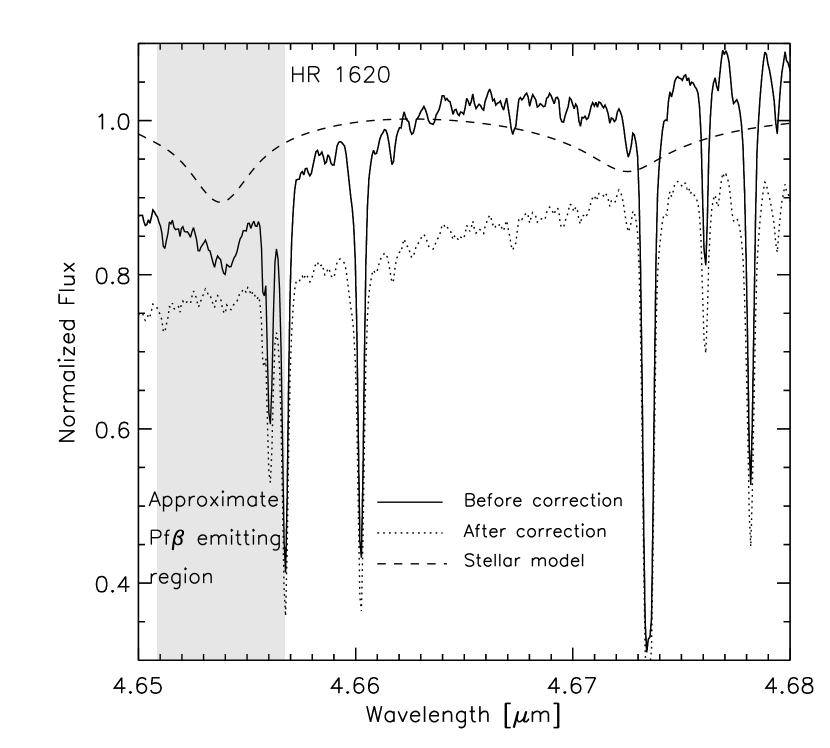
Figure 1.— Solid and dotted lines show sample standard-star spectrum before and after stellar atmospheric model division. The shaded region marks an approximate location for Pf$\beta$ emission, assuming a width of 190 km s^-1. The actual region will depend on the line width and relative radial velocity between the source and the standard stars.

Since the primary observational target of these surveys, CO, can overlie telluric CO absorption lines, targets were typically observed on two or more dates, and spectra combined to create complete CO line profiles. The H i line emitting regions are relatively unaffected by telluric absorption and so the repeated observations simply increase the S/N in these lines. Alternatively, multiple epochs can also be left separate to investigate accretion variability. This aspect of the dataset is left as future work, and will likely benefit from the inclusion of additional datasets from the NIRSPEC and CRIRES archives.

Approximate flux calibration was achieved by comparing telluric standard star spectra with literature photometry to derive a conversion from counts to flux. In all cases, the brightest observation of standard and target were utilized, as these would represent the best-centered observations. However, there is no guarantee that the sources were well centered, and the flux correction factor due to slit losses can be either greater than or less than one, depending on whether it is the source or the telluric standard that is observed off center. Nevertheless, we find decent agreement between absolute flux and literature photometry; the RMS difference between measured and literature fluxes (see Table THE SPECIAL CASE OF DOAR 21) is 50% for our sample as a whole.

Due to the inherent difficulties with absolute flux calibration for spectroscopic observations, we have chosen to correct observed fluxes with literature photometry whenever possible. The photometry used in this work can be found in Table THE SPECIAL CASE OF DOAR 21. We used M-band photometry when available, or secondarily an interpolation of other measurements, often Spitzer IRAC 4.5 and 5.8 $\mu$m fluxes. Although young stars with disks are known to have variable infrared emission, the variability is typically less than 10% for class 0-II disks (Luhman et al., 2010). Variability may be higher for transitional disks ($\sim$30-50%; Espaillat et al., 2011) and outbursting sources like EX Lup (e.g., Aspin et al., 2010), and so we note that such sources can have a corresponding systematic error in their Pf$\beta$ line flux measurement. If photometric measurements were not available in the literature, we simply used our own absolute photometry derived from the spectroscopic observations.

CRIRES reductions utilize routines written by K. Pontoppidan and described in Pontoppidan et al. (2008). 2D images for each source were added together after aligning and resampling onto a 2$\times$ finer grid. Spectra were extracted using an aperture twice the size of the FWHM of the spectral profile. As with the NIRSPEC observations, nearby telluric standards were observed close in time and airmass. Wavelength calibration was performed on the telluric standards using telluric emission lines and was applied to the target spectra after small shifts to align the spectra of target and standard.

In the nominal CRIRES reduction routines, target spectra were then simply divided by the telluric spectra to remove telluric absorption features. However, this does not account for H i absorption in the standard stars, and would have produced anomalously strong H i emission in our targets. Therefore, we implemented a routine adapted from the NIRSPEC reduction routines, which uses Kurucz photospheric models to fit and correct for H i absorption features in the standard stars.

Spectra of standard stars were also compared with literature photometry to obtain a conversion from counts to pixel, which were applied to the target spectra to obtain an approximate absolute flux calibration. However, just as with the NIRSPEC data, CRIRES flux calibration suffers from an uncertain degree of slit losses for any given observation. Therefore, as with the NIRSPEC observations, we adjusted the spectra to match literature photometry whenever possible. We find a few large discrepancies (factors of $\sim 2-3$ between literature and measured photometry, including for Elias 29, IRS 44, LLN 8, LLN 17 and WL 12. Since all show higher literature fluxes than CRIRES-measured fluxes, it is possible that this is because prior observations with the Spitzer Space Telescope or ISO included more than one source in their relatively large spatial point-spread-function. For the non-outliers, we find the RMS difference between observed and literature fluxes to be $\sim$52%.

2.3. Sample Selection

The NIRSPEC and CRIRES target lists used in this work were compiled for prior studies of M-band CO emission and do not represent an unbiased sample of young stars. However, the large sizes of these surveys means they come close to representing a complete flux-limited sample of disks with detectable CO fundamental emission in nearby clouds. The NIRSPEC M-band survey as a whole is dominated by revealed, optically thick disks, including significant numbers of both low-mass (T Tauri) and mid-mass (Herbig Ae/Be) disks. It also includes a smaller but significant number of embedded disks. The NIRSPEC sample is strongly biased against sources with tenuous disks or no disks at all, as these disks tended not to produce observable CO rovibrational emission lines. The NIRSPEC sample is also biased towards clouds at the higher declinations observable from Mauna Kea, sampling well in Taurus, Perseus, Serpens and Ophiuchus, only poorly in Lupus, and not at all at lower declinations. The NIRSPEC sample was also limited to targets with M-band continuum fluxes brighter than $\sim$0.01 Jy (M$\sim$9).

The CRIRES M-band CO survey contains many of the bright Class II disks visible from the southern sky as well as a number of Class I embedded protostars and transitional disks. This includes targets in Lupus, Vela and Chamaeleon that are difficult or impossible to observe with NIRSPEC.

A more detailed discussion of the evolutionary status of our sample as a whole is included in Section 6.4.

3. General characteristics of Pf$\beta$ detections and non-detections

A sample of targets showing different strengths and types of Pf$\beta$ emission profiles is shown for NIRSPEC in Figure 2 and for CRIRES in Figure 3. Although the biases in our sample selection make any statistics difficult to interpret, Pf$\beta$ appears to be a robust tracer of accreting systems. Greater than 80% of optically thick, classical disks around T Tauri and Herbig Ae/Be stars show detectable Pf$\beta$ emission. It is interesting to note that we find a slightly lower detection fraction for embedded protostars ($\sim 60$%). A similar fraction of embedded sources without Pf $\beta$ emission is found in a lower resolution VLT-ISAAC study of $\sim$30 sources by Pontoppidan et al. (2003, their Figures 1–7). Although the difference in detection rates may not be significant, especially because of possible biases in the selection of embedded objects, the presence of a large number of embedded protostars with little or no detectable Pf$\beta$ is interesting in and of itself. Because embedded protostars have rising continua towards the infrared, one might imagine that this could decrease line/continuum ratios and introduce an obsevational bias. However, the embedded protostars with Pf$\beta$ detections do not appear to be systematically fainter than those without, nor do the embedded protostars appear to have systematically higher M-band fluxes than the protstars with classical disks.

Figure 2.— Sample set of Pf$\beta$ emission line profiles from full NIRSPEC sample. (Note that any overlying CO emission or absorption lines have already been removed.)

Figure 3.— Sample set of profiles from full CRIRES sample. (Note that any overlying CO emission lines have already been removed.)

The majority of targets with Pf$\beta$ non-detections represent a few distinct types of objects. Not surprisingly, debris disks and disks classified as weak-line T Tauri stars (wTTS’s) or protostars with class III spectral energy distributions (SEDs) generally do not appear to show Pf$\beta$ in emission. wTTS’s with weak or non-existent Pf$\beta$ emission include HD98800 (also a circumbinary disk; Furlan et al., 2006), Hen 3-600A, LkH$\alpha$ 332 G1, TWA 7, TWA 8a and WaOph 4. These additionally show no CO fundamental emission and very low levels of veiling, likely reflecting the expected relationship between warm inner disk gas, inner disk dust, and accretion. Other targets without detectable Pf$\beta$ emission are in some way straddling the evolutionary boundary between optically thick and tenuous disks. These include HD 36917 (classified as transitioning between classes II and III in Manoj et al., 2002), CoKu Tau/3 (class II in Andrews & Williams 2005; wTTS in Furlan et al. 2011), FN Tau (classified as bordering between classical T Tauri star — cTTS — and wTTS in Furlan et al. 2011), HQ Tau (wTTS by H$\alpha$ equivalent width definitions, but cTTS according to its H$\alpha$ 10% width Furlan et al., 2011) and WSB 60 (classified as Class II in Evans et al. 2009 but shows transitional disk millimeter emission shape in Andrews et al. 2011). Other targets with no detectable Pf$\beta$ emission include the transitional disks HD 149914 (which also shows no detectable Br$\gamma$ emission; Brittain et al., 2007) as well as SR 21 (Brown et al., 2007). SR 21 has detectable CO fundamental emission, although in contrast to many other transitional disks, the emission arises from moderately large disk radii ($\sim$ 5–8 AU; Salyk et al., 2011; Pontoppidan et al., 2011b). Two circumbinary disks, CoKu Tau/4 (7.8 AU; Ireland & Kraus, 2008) and ROXs42c (23 AU; Kraus et al., 2011), also do not show Pf$\beta$ emission, although it should be noted that this does not appear to be universally true, as close binary DP Tau (projected separation 15.5 AU Kraus et al., 2011) has detectable Pf$\beta$ emission. A final interesting set of objects that universally shows no detectable Pf$\beta$ emission is the set of FU Orionis stars.

It is interesting to ask whether any classical, optically thick disks show no detectable Pf$\beta$ emission, either to test whether Pf$\beta$ could be unreliable as an accretion tracer, or to search for unique targets with optically thick disks but no accretion. The list of disks with class II SEDs that do not show Pf$\beta$ emission above detectable limits include c2dJ033035.92+303024.4, HK Tau, IRAS 03380+3135, IRAS 04385+2550, LkH$\alpha$ 270, LkCa 8, LkH$\alpha$ 325 and WaOph 5. The first five show no apparent CO emission, while the final three targets show weak CO fundamental emission, and their spectra suggest the possible presence of Pf$\beta$ at low S/N; therefore, these suggest the presence of inner disk gas. Few disks are seen with strong CO fundamental emission and no detectable Pf$\beta$ emission, one exception being the transitional disk SR 21. Very low accretion rates are also apparently not detectable in our sample. For example, the spectroscopic binary Hen 3-600A, accreting at a rate of $\sim 5\times 10^{-11}M_{\odot}\mathrm{yr}^{-1}$ (Muzerolle et al., 2000), does not have detectable Pf$\beta$ emission.

We investigated but did not determine any relationship between line shapes or widths and any other stellar or disk parameters, except that sources with double-peaked line profiles (including CI Tau, HD 141569 A, RY Tau and SU Aur) tend to have moderately high disk inclinations (typically 50-60^∘). A full discussion of the relationship between CO vibrational emission and Pf$\beta$ emission is left as future work. Here we focus on targets with detectable Pf$\beta$ emission, in order to measure mass accretion rates. Therefore, for this study we have selected a subset of the full NIRSPEC and CRIRES samples via visual confirmation of the presence of Pf$\beta$ emission. The complete target list used in this study, with relevant stellar parameters, is shown in Table THE SPECIAL CASE OF DOAR 21.

Pf$\beta$ lines are unresolved in all natural-seeing NIRSPEC observations, constraining the emission to radii less than $\sim$50 AU for typical seeing and stellar distances. Pf$\beta$ observations are also unresolved in the adaptive optics corrected CRIRES spectra. With a typical point spread function core of 0.18”, this constrains the Pf$\beta$ to radii less than $\sim$ 13 AU at 140 pc. This is consistent with an accretion origin for Pf$\beta$, as opposed to an outflow origin.

4. DERIVATION OF Pf$\beta$ LINE LUMINOSITIES

4.1. CO Emission Corrections

The Pf$\beta$ line center is close to a number of CO vibrational lines, including $v=1\rightarrow 0$ R(0) (4.6575 $\mu$m) and R(1) (4.6493 $\mu$m), $v=2\rightarrow 1$ R(8) (4.6523 $\mu$m) and ¹³CO R(14) (4.6572 $\mu$m) and R(15) (4.6504 $\mu$m). A majority of Pf$\beta$ profiles are affected by at least one of these CO features, which contain non-negligible amounts of flux. A number of techniques were utilized to correct for the CO emission, as demonstrated in Figure 4. If possible, CO lines were removed via subtraction of a Gaussian fit to the CO emission lines. In cases where the fits were not reliable, the line was replaced by a linear interpolation of the surrounding flux. In some cases, the nearby $v=2\rightarrow 1$ or ¹³CO lines contributed so significantly to the flux that it was difficult to separate the CO and Pf$\beta$ contributions. In such cases, an adjacent CO line would be shifted to the contaminating line location and subtracted. This necessarily introduces some error (of order 10%) due to the fact that the flux in adjacent CO lines may not be identical. However, more precise modeling to derive these CO line fluxes was not pursued, due to severe blending of the $v=2\rightarrow 1$ and ¹³CO rotational ladders with the much stronger $v=1\rightarrow 0$ emission lines.

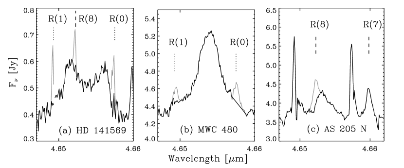
Figure 4.— Gray and black lines show sample spectra before and after removal of CO emission lines, respectively. Dotted lines mark CO $1\rightarrow 0$ lines; dashed lines mark CO $2\rightarrow 1$ lines. (a) Lines are removed with Gaussian fits. (b) R(0) is removed with a linear fit to the underlying spectrum. (c) R(8) is removed by using a Gaussian fit to R(7).

4.2. Flux Extraction

Observed Pf$\beta$ line profiles are typically not described by a Gaussian or other simple functional form, and so we chose to extract fluxes by summing all flux within a defined window, after subtraction of the continuum. The extraction window and continuum level were both determined by eye, and have associated systematic uncertainties. These can be particularly high if a number of adjacent CO lines makes the continuum hard to define, and/or if the Pf$\beta$ profile has broad wings. The sample overlap between NIRSPEC and CRIRES allows us to estimate this uncertainty to some degree, by comparing the fluxes derived from each dataset. We find good agreement between extractions using the two datasets, with typical differences less than a factor of two. Note that since the Pf$\beta$ line luminosity or the underlying continuum can be variable, some of this difference could be attributable to real changes that occurred between the two sets of observations. In our most egregious case, HL Tau, we find a factor of 3 discrepancy between the two datasets. This extreme case is illustrated in Figure 5, showing how uncertainty in both the continuum position and the position of the Pf$\beta$ line wings results in large flux differences between the two extractions.

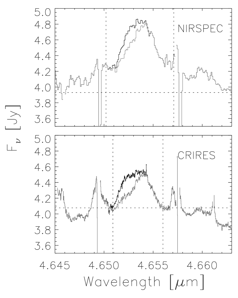
Figure 5.— Pf$\beta$ line profiles from HL Tau observed by NIRSPEC and CRIRES before (black) and after (gray) CO emission removal. Dotted lines mark the regions chosen for flux extraction, demonstrating how uncertainty in the continuum level and line width can in extreme cases result in a factor of three difference in extracted line flux.

A few of the photometrically-corrected NIRSPEC line profiles are shown in Figure 6; the remaining NIRSPEC and CRIRES profiles are available in the on-line version of the article. Our derived Pf$\beta$ luminosities, computed using the distances in Table THE SPECIAL CASE OF DOAR 21, are listed in Table THE SPECIAL CASE OF DOAR 21. Line luminosities have also been corrected for extinction, assuming an extinction of $0.034\times A_{V}$ (Cardelli et al., 1989) at 4.6538 $\mu$m, and the visual extinctions in Table THE SPECIAL CASE OF DOAR 21; if the extinction is not known, we do not include any correction. Note that even the maximum extinction in our sample ($A_{V}=34$) only results in a change in line flux by a factor of $\sim$ 3, and thus computation of Pf$\beta$ luminosity is relatively insensitive to extinction. When both NIRSPEC and CRIRES data were available, we show the average of those measurements.

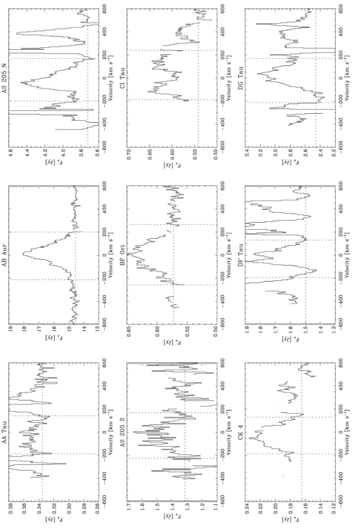
Figure 6.— Pf$\beta$ line profiles observed with NIRSPEC, after correction for CO emission and literature photometry, when available. Dotted lines mark the baseline and limits used for flux extraction. The full set of NIRSPEC and CRIRES line profiles is available in an online version of this figure.

4.3. Importance of Photospheric H I Absorption

While accretion flows are believed to be the source of the Pf$\beta$ emission, the observed spectra also include a contribution from the underlying stellar photosphere of the star/disk system. As we will discuss in this section, the correction for the underlying stellar photosphere should in nearly all cases be insignificant compared to other uncertainties, and we therefore do not apply any correction to most sources. (Note that this correction is distinct from the correction for Pf$\beta$ absorption in the photosphere of the telluric standard star, which is always corrected for in the data reduction process).

Stellar photospheres have H i absorption features that will tend to reduce the amount of observed Pf$\beta$ flux, i.e. Pf$\beta$ fluxes must be increased somewhat to correct for stellar absorption. The degree of correction depends sensitively on the stellar spectral type and veiling. Figure 1, panels a–e, show synthetic spectra and observed spectra for five spectral types (A0V – M0V), demonstrating that the absorption is most prominent at early spectral types. However, M-band veiling values for optically thick disks act in the opposite sense, with much higher veiling around early-type stars. Thus optically thick disks have negligible corrections to Pf$\beta$ from underlying stellar absorption. Synthetic veiled spectra with veiling values typical of optically thick disks ($r=46$, 18, 10, 7 and 3 for spectral types A–M, derived from disk SEDs produced with RADMC; Dullemond & Dominik, 2004) are shown as dotted lines, and are indistinguishable from straight lines.

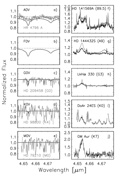
Figure 7.— Panels a)-e) show synthetic stellar H i absorption spectra without (solid curves) and with (dotted curves) the addition of typical veiling from an optically thick disk. Panels a), c), d) and e) additionally show observed spectra of unveiled stars, with the K4 and M0 spectra demonstrating that the spectra of cool stars are dominated by a molecular pseudo-continuum. Panels f)-j) show example spectra (black) and worst-case Pf$\beta$ flux corrections (i.e., assuming no veiling; gray) for the following targets: f) transitional disk HD 141569 A, g) Herbig Ae/Be star HD 144432 S, h) transitional disk LkH$\alpha$ 330, i) cTTS DoAr 24 ES and j) transitional disk GM Aur.

Stars with G–M spectral types have M-band spectra that are dominated by a molecular pseudo-continuum, rather than simply H i absorption (see panels c, d and e), which can result in some change to Pf$\beta$ flux due to coincident molecular absorption features near Pf$\beta$. The equivalent width of the underlying photospheric features drop by a factor of $1+r$ where $r$ is the veiling (defined as the dust continuum flux density divided by the stellar photospheric flux density). Considering the spectrum of HD 79210 shown in Figure 1, a reasonable M-band veiling value of $\sim$3 for an optically thick disk reduces the strongest photospheric features to the $\sim 7\%$ level; this and their narrow width results in a negligible correction for optically thick disks.

Transitional disks — disks with inner regions depleted of small dust grains — have low continuum fluxes, and so could potentially have large relative contributions from the underlying photosphere. However, we find that such targets (see Figure 1 panels f), h) and j)) often have high line/continuum ratios, likely because in spite of their lowered near-IR continuum fluxes, transitional disks have only slightly lowered accretion rates (Najita et al., 2007). (See extended discussion in Section 6). As examples, corrections to the Pf$\beta$ flux due to photospheric H i from transitional disks HD 141569 A, LkH$\alpha$ 330 and GM Aur, (panels f, h and j) would be only $\sim$ 20, 45 and 3%, respectively, even in the worst case scenario (no veiling). Actual corrections for these sources should be a factor of a few lower, due to non-zero M-band veiling (Salyk et al., 2009). The molecular photospheric absorption features might be more problematic, but luckily the spectra can be examined at other wavelengths to determine whether there is likely significant contamination from the underlying photosphere. With visual examination, we found one target — DoAr 21 — which shows both low Pf$\beta$ equivalent width and low veiling, and in this case the molecular absorption features in its stellar photosphere have a non-trivial effect on the determination of the disk Pf$\beta$ line flux. We describe this example in detail in an Appendix.

The largest possible correction would be required for a naked A or F star with a low Pf$\beta$ line/continuum ratio (see, e.g., panel g), perhaps doubling the ratio of true to observed Pf$\beta$ emission flux. Such a target would be difficult to identify because its relatively featureless M-band spectrum looks the same whether it is naked or veiled. To our knowledge, there are no known diskless targets in our sample that also show detectable Pf$\beta$ emission. Of course, stellar Pf$\beta$ absorption could erase signatures of weak Pf$\beta$ emission from weakly-accreting disks; however, we have no good way to pinpoint such targets. A possible example of such a target could be SR 21 (see Figure 2) a G2.5 star with a transitional disk, which has CO gas at $\sim$7 AU but no measurable accretion (Pontoppidan et al., 2008).

5. Pf$\beta$ LUMINOSITY AND ACCRETION RATES

5.1. Correlation between Pf$\beta$ Luminosity and Accretion Luminosity

In Figure 8, we show the correlation between our measured Pf$\beta$ line luminosities and previously-measured accretion luminosities, listed in Table THE SPECIAL CASE OF DOAR 21. We chose to maximize the number of sources in this correlation and, therefore, the literature accretion luminosities are derived from a variety of observational methods. The majority are derived from models and observations of the UV excess continuum, while others are derived somewhat less directly from UV data, utilizing a relationship between mass accretion and the Balmer discontinuity (Muzerolle et al., 2004) or approximating the UV excess using photometry. About a third of the accretion rates are derived from empirical relationships between H i emission lines (Br$\gamma$ or Pa$\beta$) and accretion luminosity. Although the Br$\gamma$ and Pa$\beta$-derived accretion rates are themselves an indirect measure of accretion rate, we find no significant biases between these and the UV-derived accretion luminosities in Figure 8.

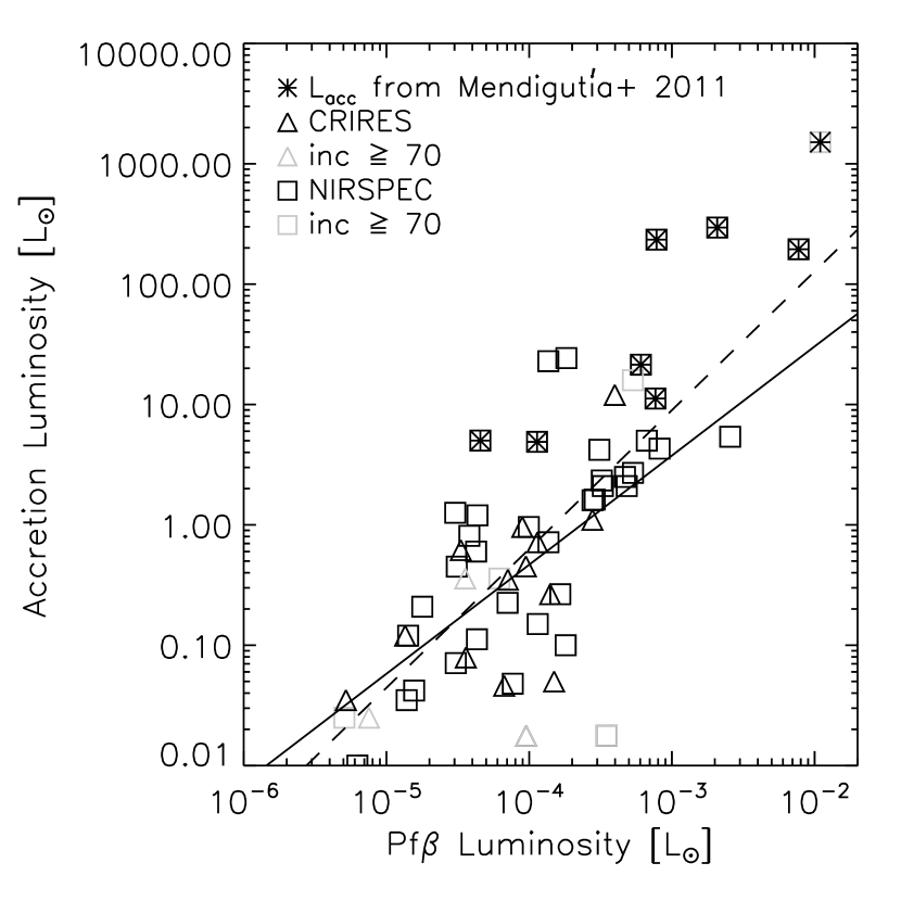
Figure 8.— Correlation between literature accretion luminosity (see Table THE SPECIAL CASE OF DOAR 21) and Pf$\beta$ luminosity (this work). If Pf$\beta$ is measured by both NIRSPEC and CRIRES, we show two symbols (squares and triangles, respectively) on the plot. Sources with high inclination or otherwise unreliable accretion rates (in gray) are excluded from the correlation analysis. The solid line shows the best linear fit to the data excluding points from Mendigutía et al. (2011) (Equation 1). The dashed line shows the best linear fit including points where $L_{\mathrm{acc}}$ is derived from Mendigutía et al. (2011).

Because the accretion rates of high-inclination sources can be unreliable, we remove these from our correlation. We also omit HL Tau from the correlation; although its disk appears to be viewed at moderate inclination (Kwon et al., 2011), its high level of veiling makes literature accretion rates very uncertain (e.g., White & Ghez, 2001).

We find that the correlation between Pf$\beta$ line luminosity and accretion luminosity is heavily influenced by targets with high accretion luminosities derived by Mendigutía et al. (2011). Mendigutía et al. (2011) derived accretion rates in 38 HAeBe stars by estimating the Balmer excess using U- and B-band photometry compared with accretion shock models. Since accretion rates correlate with stellar mass, these accretion rates populate the upper right corner of Figure 8. If these points are included in the fit, we find that our correlation then poorly reproduces previously-measured accretion rates for low-mass stars. Indeed, Mendigutía et al. (2011) note a change in the slope of the correlation between accretion rate and stellar mass between low-mass and high-mass stars, and find larger accretion rates than those determined from Br$\gamma$ emission lines (Garcia Lopez et al., 2006), implying that correlations between accretion tracers and accretion rates may not extend linearly to higher mass stars. However, UV excesses are significantly more difficult to measure around high-mass stars, and additional study is warranted to understand whether the emission line-accretion luminosity relationship needs to be modified at higher stellar masses. Therefore, in this study, we omit the accretion luminosities derived by Mendigutía et al. (2011) from our analysis. If the results of Mendigutía et al. (2011) are correct, our study will tend to underestimate accretion luminosities for $M_{\star}\gtrsim 3M_{\odot}$.

Excluding the accretion luminosities in Mendigutía et al. (2011), we find the following relationship between Pf$\beta$ luminosity and previously-measured accretion luminosities:

$$\log{L_{\mathrm{acc}}[L_{\odot}]}=(0.91\pm 0.16)\times\log{L_{\mathrm{Pf\beta}}[L_{\odot}]}+(3.29\pm 0.67).$$ (1)

5.2. New Accretion Rates

We use Equation 1 to compute accretion luminosities for our entire sample. These are listed in Table THE SPECIAL CASE OF DOAR 21. An estimate of $\dot{M}$ is derived using the standard relationship between $L_{\mathrm{acc}}$ and $\dot{M}$:

$$L_{\mathrm{acc}}=0.8\,GM_{\star}\dot{M}/R_{\star}$$ (2)

from Gullbring et al. (1998). $M_{\star}$ and $R_{\star}$ are taken from Table THE SPECIAL CASE OF DOAR 21. If not shown in Table THE SPECIAL CASE OF DOAR 21, $R_{\star}$ is derived from $L_{\star}$ and $T_{\star}$ assuming $L_{\star}=4\pi R_{\star}^{2}\sigma T_{\star}^{4}$. We do not compute $\dot{M}$ if these parameters are not available. However, $\dot{M}$ could easily be computed at a later time when these parameters are measured.

In Figure 9, we show accretion rates derived here compared to existing values from the literature (Table THE SPECIAL CASE OF DOAR 21). The accretion rates derived here show no systematic bias, and most accretion rates are within 0.5 dex of previous measurements. The standard deviation of the current and previous measurements is 0.77 dex. These results are similar to those for other emission line accretion tracers, albeit over a somewhat more limited range of accretion rates. For example, Herczeg & Hillenbrand (2008) quote standard deviations of 1.0, 0.71 and 1.1 dex between UV continuum excess and Ca ii $\lambda$8542, Ca ii $\lambda 8662$ and He I $\lambda 8576$, probing accretion rates as low as $10^{-12}M_{\odot}\mathrm{yr}^{-1}$. In addition, Herczeg & Hillenbrand (2008) estimate a factor of 4 (0.6 dex) random error in UV excess measures alone, due to errors in extinction and distance. Also, accretion rates are known to be variable, with Nguyen et al. (2009) finding typical accretion rate variations of 0.35 dex, but variations commonly as high as 0.5 dex. Therefore, Pf$\beta$ appears to be an accretion tracer on par with existing tracers, with scatter not much larger than what would be expected from accretion variability and errors related to the derivation of UV-based accretion luminosities.

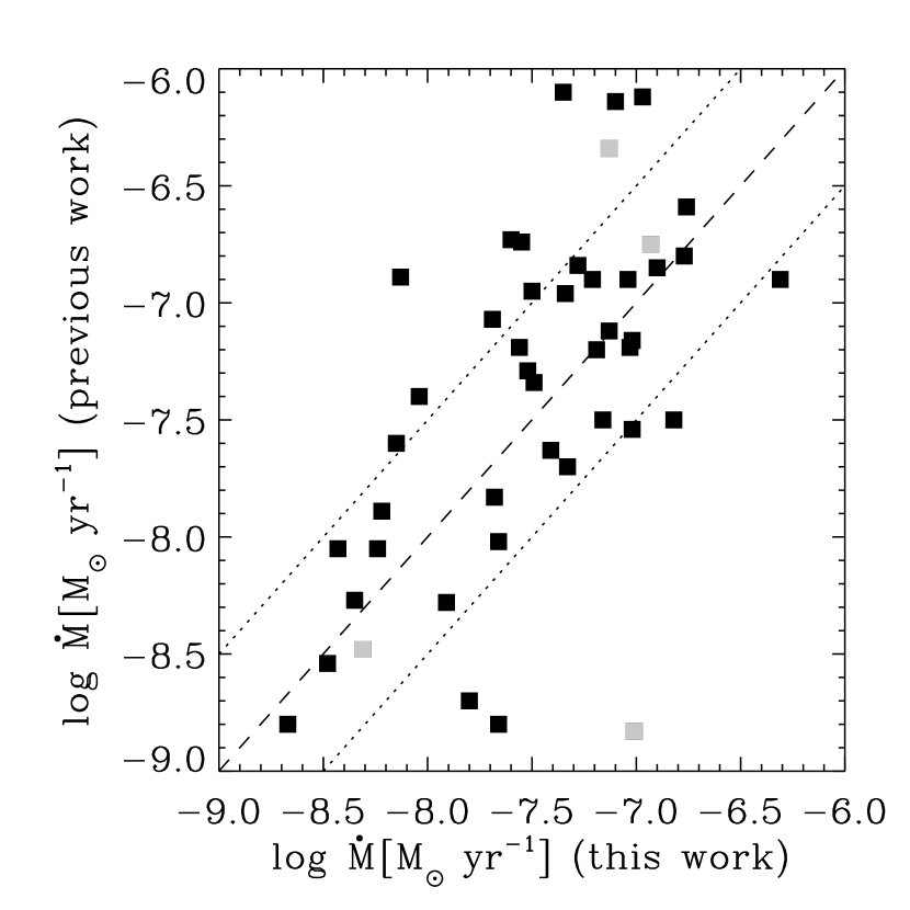
Figure 9.— Mass accretion rates derived from this work compared with values from the literature. High-inclination disks are shown plotted in gray. The dashed line shows a 1:1 correlation and dotted lines show a difference of 0.5 dex.

5.3. About Upper Limits

Computing upper limits on the Pf$\beta$ line flux, and thus accretion rate, for any given source is not straightforward, and because these are not crucial for the work presented here, we do not make an attempt to compute them. Complications include the fact that the Pf$\beta$ line shapes are complex, and their widths varied, so the correct choice of assumed lineshape and width is not obvious. In addition, sources with no detectable Pf$\beta$ emission are often less-heavily veiled sources, whose underlying photospheres must be modeled to derive an accurate Pf$\beta$ flux. We encourage those interested in an upper limit for a particular source in the NIRSPEC or CRIRES archives to contact the authors of this work to discuss whether reasonable assumptions can be made to derive limits for this source.

Nevertheless, we can make some general observations about how sensitive Pf$\beta$ measurements are to accretion rates. Assuming the Pf$\beta$ line is a Gaussian with $\sigma_{width}=0.001\mu\mathrm{m}$ (derived from a fit to AB Aur’s Pf$\beta$ emission line), then with a continuum flux density of $F_{\nu}=1$ Jy, a signal-to-noise ratio (SNR) of 50, a 3$\sigma$ line peak, and for a 1 solar mass, 1 solar radius star, the minimum measurable accretion rate is $\sim 4\times 10^{-9}M_{\odot}\mathrm{yr}^{-1}$. The minimum measurable accretion rate then scales roughly proportional to $\frac{F_{\nu}}{SNR}$. For the integration times used for the acquisition of the data used in this work, Pf$\beta$-derived accretion rates do not appear to be as sensitive as previous studies using Br$\gamma$ or Pa$\beta$ (e.g., Natta et al., 2006).

The lowest detected accretion rates in our sample are for the transitional disks TW Hya and DM Tau, with rates of $2.6\times 10^{-9}$ and $4.3\times 10^{-9}M_{\odot}\mathrm{yr}^{-1}$, respectively. Pf$\beta$ is especially well-suited for measuring small accretion rates from transitional disks, as the dust-cleared inner holes decrease $F_{\nu}$ and increase the line/continuum ratio (see Section 6.2 for more detail). However, as the SNR per unit exposure time also decreases as $F_{\nu}$ decreases, sufficient time must be expended to reach a reasonable SNR.

6. ANALYSIS AND DISCUSSION

6.1. Utility of Pf$\beta$ and Comparison to Other Accretion Tracers

In this work, we have introduced the use of H i Pf$\beta$ to measure mass accretion from protoplanetary disks. Although numerous accretion tracers have been developed prior to this work, the use of Pf$\beta$ offers several advantages, which we outline here.

One major advantage of using Pf$\beta$ as an accretion tracer is that it comes “for free” and contemporaneous with observations of CO fundamental emission. The NIRSPEC and CRIRES surveys from which we extract the data in this work provide a self-consistent sample of accretion luminosity estimates for 120 targets, and the NIRSPEC and CRIRES archives likely include many additional protoplanetary disk targets for which accretion luminosities could be estimated. To our knowledge, this is the first work to make extensive use of M-band spectra of protostars from both NIRSPEC and CRIRES — data which are all currently available in their respective archives. The varied and large set of targets resulting from this combined dataset is a great demonstration of the utility of these large archives. As future work, we plan to extend our analysis to investigate long-term ($\sim$year timescales) accretion variability for different classes of disks.

The simultaneous observation of CO and Pf$\beta$ also allows for a comparison between the accretion flow and molecular disk gas at distances of $\sim$ 0.1–1 AU from the star (e.g., Pontoppidan et al., 2011b; Salyk et al., 2011), which is traced by CO fundamental emission. The relationship between these two disk components is being investigated, e.g., by Brown et al., submitted . The contemporaneous nature of these measurements also allows for simultaneous measurements of disk gas and accretion rate as a function of time, although it should be cautioned that there can be changes in emission line fluxes without corresponding changes in accretion rate (e.g., Gahm et al., 2008). The tidal influence of protoplanets is predicted to cause CO emission line variability (Regály et al., 2011), but understanding the influence of proto-planets requires ruling out other possible sources of line variability, such as changes in accretion rate or accretion geometry.

Pf$\beta$ (n=7$\rightarrow$5) is in many ways similar to Br$\gamma$ (n=7$\rightarrow$4; 2.160 $\mu$m), originating from the same upper level energy and appearing in the infrared. In Figure 10, we compare Pf$\beta$ EW with literature values of EW(Br$\gamma$) as well as EW(Pa$\beta$) (see Table THE SPECIAL CASE OF DOAR 21). Typical values of Pf$\beta$ equivalent widths are between 1/3 and 3 $\times$ EW(Br$\gamma$) or EW(Pa$\beta$), with EW(Pf$\beta$) typically being similar to EW(Br$\gamma$) but somewhat smaller than EW(Pa$\beta$). The lack of a strong correlation between tracers likely reflects the varied temperatures of the accretion column, the underlying photosphere, and the continuum veiling. Muzerolle et al. (1998), Calvet et al. (2004) and Donehew & Brittain (2011) all find correlations between accretion luminosity and Br$\gamma$ luminosity very similar to our Equation 1. Equation 1 combined with the relationships in Muzerolle et al. (1998) and Donehew & Brittain (2011) predict somewhat higher EW(Pf$\beta$) than EW(Br$\gamma$), while the relationship in Calvet et al. (2004) predicts somewhat lower EW(Pf$\beta$) as compared to EW(Br$\gamma$) (with differences less than $\sim 0.2$ dex). Lineshapes of the two accretion tracers appear to be quite similar — typically single-peaked with line widths near $\sim$ 200 km s^-1 (Garcia Lopez et al., 2006). HD 141569 A, on the other hand, is an example of a disk with both double-peaked Br$\gamma$ and Pf$\beta$ emission lines. Interestingly, however, several targets for which Pf$\beta$ is clearly in emission show no Br$\gamma$, or Br$\gamma$ in absorption — for example, HD 142527, HD 142666, T CrA and TY CrA. Thus, Pf$\beta$ may be a more robust accretion tracer in targets with low near-IR veiling.

Figure 10.— EW of Pf$\beta$ compared to those of Br$\gamma$ (bottom) and Pa$\beta$ (top). The outliers with highest Pf$\beta$ EW in the bottom plot are transitional disks HD 141569 A, GM Aur and TW Hya.

Although equivalent widths are similar, Pf$\beta$ offers some distinct advantages over Br$\gamma$ and Pa$\beta$. One advantage is the relatively higher continuum veiling in the M band as compared to shorter wavelengths. Since the photospheric emission is a smaller fraction of the total flux at 5 $\mu$m than it is at shorter wavelengths, Pf$\beta$ suffers less contamination and uncertainty from the underlying photospheric H i absorption (as discussed in detail in Section 4.3). Being at longer wavelengths also makes Pf$\beta$ less sensitive to extinction. Using the reddening law of Cardelli et al. (1989), $A_{\mathrm{Br\gamma}}/A_{V}=0.12$ while $A_{\mathrm{Pf\beta}}/A_{V}=0.03$, a factor of 4 difference in magnitudes of correction. At $A_{V}\sim 30$, for example, this results in a flux correction factor of $\sim$ 28 for Br$\gamma$ but only $\sim$3 for Pf$\beta$. Finally, Pf$\beta$ equivalent widths are quite high for accreting disks with low continuum veiling; thus, Pf$\beta$ is an excellent tracer for low accretion rates in disks with inner regions depleted in small dust grains (discussed further in Section 6.2). One disadvantage of Pf$\beta$ as an accretion tracer is the systematic errors that are introduced by complex CO emission/absorption spectra, which can result in up to a factor of a few uncertainty in flux in extreme cases (as in Figure 5). Another is that the veiling is difficult to determine empirically in earlier-type stars with few photospheric features, and so the importance of H i stellar photospheric absorption is difficult to assess in these stars (see Section 4.3).

6.2. Accretion in Transitional Disks

6.2.1 Equivalent Widths and the Identification of Transitional Disks

In Figure 11 we show Pf$\beta$ equivalent width (EW) vs. Pf $\beta$ luminosity. There is no significant correlation between these two variables and thus Pf$\beta$ EW is not a good predictor of accretion luminosity. However, we note that several transitional disks have notably high Pf$\beta$ EW’s (between $-20$ and $-30$ Å). Since the Pf$\beta$ luminosities of these disks are not higher than average, the high EW’s instead reflect the fact that these disks have reduced continuum flux levels in the near-IR. This suggests that Pf$\beta$ may be a good tracer for some accreting transitional disks, and a means to detect these disks with a single spectrum — one simple, robust measurement that requires no knowledge of the stellar parameters or absolute flux level. We arbitrarily label all disks with Pf$\beta$ EW $<-15$ and suggest that these targets may have depletions of dust in their inner regions. Aside from the transitional disks, which are known to have inner disk dust depletions, we also note that TY CrA is a tertiary system with an eclipsing binary (e.g., Vaz, 2001) and that Haro 1-1 is an anomalously fast rotator (Shevchenko & Herbst, 1998). To our knowledge, no unique properties have been discussed for the other disks with high Pf$\beta$ EW.

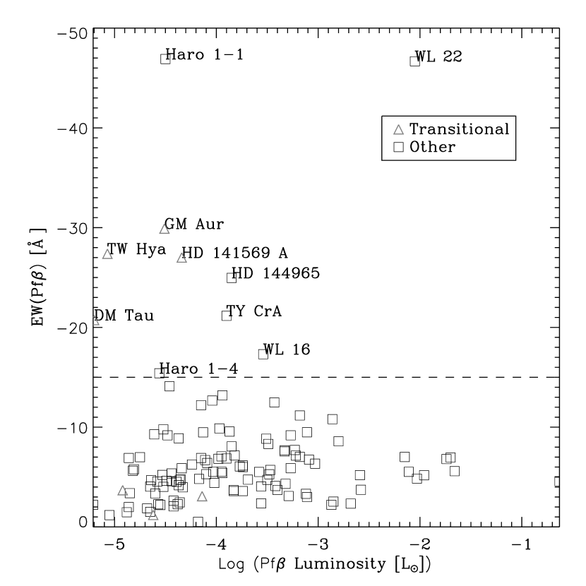
Figure 11.— Pf$\beta$ equivalent width (EW) plotted against Pf$\beta$ line luminosity. Note that EW is not a good predictor for Pf$\beta$ luminosity (or therefore accretion luminosity). The dashed line marks an EW of $-15$ Å; several transitional disks have extreme values of Pf$\beta$ EW.

It is interesting to note that Pf$\beta$ EW’s are not high for all transitional disks. In our sample, LkH$\alpha$ 330, HD 135344 B, IRS 48 and DoAr 44 have typical or even slightly low Pf$\beta$ EW’s. LkH$\alpha$ 330 and HD 135344 B appear to have relatively low gas/dust ratios as compared to other transitional disks (Salyk et al., 2009). DoAr 44 might better be considered a pre-transitional disk (Andrews et al., 2011) — a disk with an inner clearing but relatively high near-IR flux, that may be consistent with a small gap rather than a large clearing (Espaillat et al., 2007). And IRS 48 has a $\sim$ 30 AU hole in its gas distribution (Brown et al., 2012). Therefore, high Pf$\beta$ EW may be an indicator of only those transitional disks that have significantly cleared their inner regions of small dust grains but not gas. Thus, a measurement of Pf$\beta$ EW might shed light on the process causing the inner disk depletion for any given disk, as different clearing scenarios predict different gas/dust ratios.

6.2.2 Transitional Disks in Comparison to Other Disks

Figure 12 shows the log of Pf$\beta$ luminosity as a function of the log of stellar mass. Accretion luminosity and accretion rate are known to scale with stellar mass, and these results are no exception. Plotting Pf$\beta$ luminosity as a function of stellar mass allows us to investigate potential outliers with high or low accretion rates.

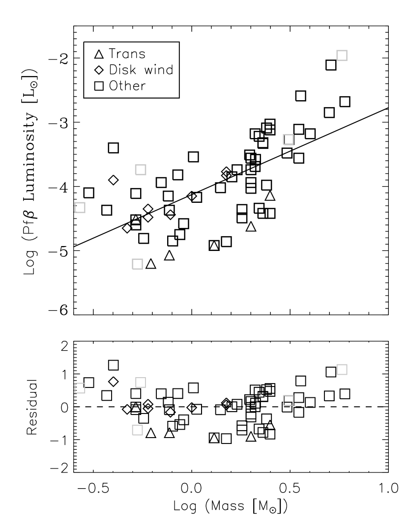
Figure 12.— The top panel shows the log of Pf$\beta$ line luminosity plotted against the log of stellar mass and best-fit correlation. The lower panel shows the fit residuals. Triangles and diamonds are transitional and disk wind targets, respectively; squares are other targets. Gray squares represent highly-inclined disks.

Transitional disks have on average lower Pf$\beta$ luminosities, at a marginally statistically-significant level, with a mean log residual Pf$\beta$ luminosity of $-0.7\pm 0.3$. A low Pf$\beta$ luminosity could represent a low accretion luminosity, or could result if the transitional disks have normal accretion luminosities but an anomalously low Pf$\beta$ luminosity/accretion luminosity ratio. However, we have investigated the Pf$\beta$ luminosity/accretion luminosity ratio for these targets and find that 4 of 5 transitional disks with literature accretion luminosities (DM Tau, GM Aur, HD 141569 A and TW Hya) have Pf$\beta$ luminosities even higher than would be predicted by Equation 1 (one, HD 135344 B, has a slightly but not significantly lower Pf$\beta$ luminosity). Therefore, this study is in closer agreement with Najita et al. (2007) and Espaillat et al. (2012) who find slightly lower than average accretion rates for transitional disks, than with contrasting studies showing no difference between the two types of disks (Fang et al., 2009; Sicilia-Aguilar et al., 2010). As suggested by (Sicilia-Aguilar et al., 2010), the contrasting study results may be due to the different physical nature of transitional disks in different regions. However, it should be cautioned that the high Pf$\beta$ EW’s for transitional disks could produce an observational bias in our work, making it easier to detect a low accretion rate around a transitional, rather than classical, disk. Thus, our sample may be missing a number of classical disks with low accretion rates.

Since our sample derives from a large number of clusters of different ages, it is also worth asking whether we might measure spuriously low Pf$\beta$ luminosities for transitional disks because they are derived from older clusters, and there is evidence that accretion rates decrease with stellar age (Hartmann et al., 1998). However, we find that the transitional disks are derived from a large number of the clusters sampled in this work, and that regardless of the cluster under consideration, transitional disks lie at the low end of the range of measured Pf$\beta$ luminosities. In addition, the transitional disks are derived primarily from clusters with ages $\lesssim 3$ Myr (with the exception of TW Hya), and so are not biased towards older ages.

6.3. Accretion in Disk Wind Sources

Disk wind targets are a newly identified subset of disks defined by their single-peaked near-IR emission line flux and spectro-astrometric profiles, which may be evidence for the presence of a slow-velocity disk wind (Pontoppidan et al., 2011b; Bast et al., 2011). By comparing average accretion luminosities for disk wind and normal disk targets, Bast et al. (2011) noted that disk wind targets may have higher than average accretion luminosities. However, Figure 12 shows that the Pf$\beta$ luminosities for these targets are actually typical for sources in our sample, implying no higher accretion luminosities. These targets also have typical ratios of Pf$\beta$ luminosity to derived accretion luminosity. And, the disk wind sources derive from a large number of clusters, implying no obvious age-related biases.

How can these two results be reconciled? We believe there are a few possible explanations. Firstly, the disk wind sources in Bast et al. (2011) have somewhat higher stellar masses than their comparative sample of “normal” disks. Secondly, the disks in the comparative sample in Bast et al. (2011) have lower accretion luminosities at a given mass than disks in our sample. Since our full sample has not been “vetted” for disk wind targets, it is possible that our full sample includes unidentified disk wind targets that increase the average, or our sample may simply be biased towards higher accretion rates. Unfortunately, we cannot use the criteria in Bast et al. (2011) to classify all of our targets because of the relatively lower spectral resolution of NIRSPEC as compared to CRIRES.

The accretion rates for the disk wind targets, derived from this work, range from 6$\times 10^{-9}$ to 2$\times 10^{-7}M_{\odot}\mathrm{yr}^{-1}$, with most accretion rates in the range of $10^{-8}-10^{-7}M_{\odot}\mathrm{yr}^{-1}$. Thus, the disk wind sources are likely capable of supporting mass-loss rates of $10^{-10}-10^{-9}M_{\odot}\mathrm{yr}^{-1}$, and in some cases $10^{-8}M_{\odot}\mathrm{yr}^{-1}$, as suggested by Pontoppidan et al. (2011b).

Although we find typical accretion rates for disk wind sources, it should be noted that one of the primary characteristics of disk wind targets is their high veiling at optical through IR wavelengths (e.g., Gahm et al., 2008). The seemingly contradictory observation of high veiling but normal accretion rates may be reconciled by the results of Gahm et al. (2008), who find that the optical veiling in such targets is not a good measure of disk accretion, as the derived optical veiling is affected by infilling of photospheric lines from line emission.

6.4. Accretion Rates for Embedded Disks

6.4.1 Classification of Evolutionary Stage

The process of star and planet formation is often deconstructed into four discrete evolutionary stages. The targets in our sample represent primarily, if not entirely, sources in stages I and II, where stage I sources are embedded protostars with still-collapsing envelopes, while stage II sources are revealed stars with circumstellar disks and little or no remaining envelope. For this work, the evolutionary class was determined primarily through examination of the M-band spectra themselves, with stage I disks defined as those showing CO ice absorption, and stage II disks those without. This offers the significant advantage that our entire sample can be easily classified using our own dataset, with a single consistent criterion.

However, it is a known issue that edge-on stage II disks can masquerade as evolutionarily-younger systems, especially with the use of spectral slope-based classification schemes (see, for example, the detailed discussion in Evans et al., 2009). Our classification scheme is not immune to this issue, as CO ices in edge-on disks can in principle produce absorption features. However, in practice, the production of strong ice absorption features requires a very specific geometry, with an inclination close to the opening angle of the flaring disk. Additionally, the upper layers of the disk that intercept the starlight are often too warm to contain significant quantities of CO ice (Pontoppidan et al., 2005). Thus, it is perhaps not surprising that our classification scheme correctly identifies some high-inclination disks, including T Tau S and VV Ser, as stage II rather than stage I sources.

Nevertheless, we have made an effort to confirm stage I classifications whenever possible using additional diagnostics in the literature, including the use of spectral indices, bolometric temperatures, the presence of infall or outflow signatures in spectral lines, and the presence of extended envelopes as seen in millimeter-wave maps (e.g. Boogert et al., 2002; White & Hillenbrand, 2004; Doppmann et al., 2005; Evans et al., 2009; van Kempen et al., 2009; Jørgensen et al., 2009; Herczeg et al., 2011). Our classifications are listed in Table THE SPECIAL CASE OF DOAR 21, along with accompanying notes for sources with ambiguous properties.

6.4.2 Accretion Rates for Stage I Disks, and Comparison with Stage II Disks

Since stars are believed to accumulate most of their mass during their embedded stages, accretion rates for stage I disks were initially predicted to be significantly larger than for stage II disks. Smooth collapse models (Shu, 1977) predicted stage I accretion rates similar to simple estimates — for example, accretion rates of order $\gtrsim 10^{-6}M_{\odot}\mathrm{yr}^{-1}$ are required to build a solar mass star over a $\sim 10^{6}$ year timescale. Accretion rates in stage II disks around solar-mass stars are typically near $\sim 10^{-8}M_{\odot}\mathrm{yr}^{-1}$ (see Table THE SPECIAL CASE OF DOAR 21 and references therein), and thus stage I accretion rates would be predicted to be at least two orders of magnitude higher.

While there is at least some evidence for greater accretion activity in stage I sources (e.g. Doppmann et al., 2005), measured accretion rates in stage I disks around low-mass stars are found to be near $10^{-8}M_{\odot}\mathrm{yr}^{-1}$ (e.g. White & Hillenbrand, 2004; White et al., 2007) — two orders of magnitude lower than predicted. This discrepancy is related to the well-known “luminosity problem” in star formation (Kenyon et al., 1990), wherein measured bolometric luminosities (which derive primarily from the energy of gravitational contraction, and are therefore related to mass accretion) are lower than predicted from steady growth models. Instead, evidence is growing (e.g. Dunham et al., 2008; Enoch et al., 2009; Evans et al., 2009) that accretion may need to be episodic — primarily quiescent, with brief phases of intense accretion.

While direct measurements of accretion rates in stage I disks appear to support this hypothesis, such studies inevitably suffer from a bias towards more revealed disks, as the most embedded protostars are heavily extincted, and cannot be easily studied with either optical or near-IR accretion tracers. Although it is difficult to quantify the many sample-selection biases here, extinction remains small in the M band even for high $A_{V}$, and our sample includes several heavily embedded protostars. As a point of comparison, the sample of young protostars in White & Hillenbrand (2004) all have $A_{V}<20$, while 10 of 20 stage I disks in our study have $A_{V}\geq 20$. Thus, our study provides insight about accretion rates for the most embedded, and perhaps evolutionarily youngest, disks.

Figure 13 shows the empirical cumulative distributions of calculated Pf$\beta$ luminosities for stage I and stage II disks in our sample. There are small differences between the distributions of Pf$\beta$ line luminosities for the two samples, with slightly higher Pf$\beta$ luminosities in Stage II disks. Stage I disks have a mean $\log(L_{\mathrm{Pf}\beta})$ of $-3.7$ and a standard deviation of $0.8$, while stage II disks have a mean $\log(L_{\mathrm{Pf}\beta})-3.8$ with a standard deviation of 0.9. However, a two-sample Kolmogorov-Smirnov test produces an associated probability of 30%. Therefore, the hypothesis that the stage I and stage II disks draw from the same distribution of accretion luminosities cannot be rejected, i.e., differences between the two distributions are not statistically significant.

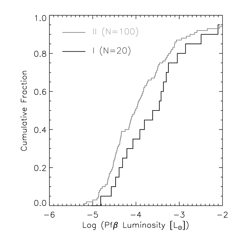
Figure 13.— The cumulative distribution function of observed Pf$\beta$ accretion luminosities for stage I and stage II disks.

Unfortunately, accretion rate distributions cannot be compared directly, as the majority of the embedded disks in our sample do not have measured stellar masses or radii due to the relative difficulty of obtaining optical spectra for highly embedded stars. However, if average stellar masses and radii are similar for the two samples our results suggest that accretion rates are quite similar for stage I and stage II disks. Spectroscopic analyses of stage I protostars have suggested that stage I and stage II stars have similar average masses, while stellar radii are no more than a factor of $\sim 2$ larger for stage I stars (White & Hillenbrand, 2004). For the small number (four) of stage I disks with measured stellar masses in our sample, the average stellar mass is $1.7M_{\odot}$, as compared to an average of $1.8M_{\odot}$ for our stage II sample. Assuming at most a factor of two difference in radius between stage I and II stars, and assuming no signficantly different selection biases for our two subsamples, our results suggest that stage I accretion rates are at most factors of a few higher, on average, than they are for stage II disks.

We can directly measure the accretion rates of four stage I targets in our sample. These accretion rates range from $1\times 10^{-8}$ to $4\times 10^{-7}M_{\odot}\mathrm{yr}^{-1}$. Thus, these targets have an accretion rate spread of more than an order of magnitude, spanning from a value typical for low-mass stars to something close to the $10^{-6}M_{\odot}\mathrm{yr}^{-1}$ required to build a solar mass star in 1 Myr. If we divide the currently-measured stellar mass by $\dot{M}$, we can obtain a lower limit to the time required to form the star assuming a steady state accretion rate. We find timescales of 0.7, 6, 54 and 67 Myr for the four stage I sources — longer than estimated stage I lifetimes (Evans et al., 2009). Therefore, our data suggest that these sources must at times have had significantly higher accretion rates than currently observed.

Making some simple assumptions, we can also investigate accretion rates for the full stage I sample. For example, assuming $M_{\star}=1M_{\odot}$ and $R_{\star}=2R_{\odot}$ for the 16 stage I stars without measured stellar parameters, we find a mean and standard deviation of $\log(\dot{M})=-7.1\pm{0.7}$. This value is at least an order of magnitude lower than the predictions from steady accretion models. Yet, with these assumptions, our sample does include two sources with accretion rates of $\sim 2\times 10^{-6}M_{\odot}\mathrm{yr}^{-1}$. If our sample is representative of all stage I sources and homogeneous except for random changes in accretion rate due to episodic accretion, and taking into account a detection fraction of 60% (see Section 3), this would imply that the stage I sources spend $\sim 6\%$ of their lifetime with $\dot{M}>10^{-6}M_{\odot}\mathrm{yr}^{-1}$. The large number (40%) of Pf$\beta$ non-detections is further evidence for a wide range of accretion rates in stage I sources, again consistent with an episodic accretion scenario.

It is also interesting to note that no FU Orionis stars in our sample show detectable Pf$\beta$ emission lines. The explanation for this is not known, but may have to do with the restructuring of the inner disk that occurs during high accretion-rate events (e.g. Zhu et al., 2009). In any case, while these sources may represent protostars with the highest rates of accretion (Hartmann & Kenyon, 1996), they are necessarily excluded from this analysis due to their lack of Pf$\beta$ emission, and thereby bias the remaining sample towards lower accretion rates.

7. CONCLUSIONS

In this work, we have introduced the use of H i Pf$\beta$ as a mass accretion tracer for young stars with protoplanetary disks. H i Pf$\beta$ offers several advantages over other accretion tracers, including being readily observed in heavily-extincted disks, requiring minimal correction for photospheric absorption and being commonly observed along with CO fundamental transitions. Using existing measurements of accretion from the literature, we derive a relationship between Pf$\beta$ line luminosity and accretion luminosity, and show that this relationship can reproduce measured accretion rates with an accuracy similar to that of other commonly-used tracers. Examining our large sample of accretion rates, we are further able to show that “disk wind” sources appear to have normal accretion rates, while our sample of transitional disks have slightly lower than average accretion rates.

We also examine the accretion rates of the stage I disks in our sample — a sample that includes significantly more embedded targets than in previous studies of this type. We find that stage I and stage II disks have statistically indistinguishable Pf$\beta$ luminosities, implying similar accretion rates, and that the accretion rates of stage I disks are too low to build a stellar mass with quiescent accretion. Our results instead are consistent with both observational and theoretical evidence that stage I objects experience episodic, rather than quiescent, accretion.

The calibration of Pf$\beta$ presented here has allowed for a coherent comparison of accretion luminosity in 120 stars. While this work has focused exclusively on spectra from the NIRSPEC and CRIRES surveys with which we are associated, the correlation we derive can be extended to a much larger number of protoplanetary disk spectra, including some which may already reside in the NIRSPEC or CRIRES archive. We have also focused exclusively on disks with clearly detectable Pf$\beta$ emission. However, with more extensive observations and focused analysis, our correlation can be extended to tenuous disks with low accretion rates — disks of utmost importance to our understanding of disk dissipation. Finally, as Pf$\beta$ is observed contemporaneously with CO fundamental emission lines, the observation of Pf$\beta$ can be used to account for the effects of accretion variability in searches for planet-induced CO line variability. We therefore expect the utility of Pf$\beta$ as an accretion tracer to extend well beyond the work presented here.

8. ACKNOWLEDGEMENTS

C.S. thanks Casey Deen and Chris Sneden for providing an introduction to MOOG. C.S. also acknowledges the financial support of the NOAO Leo Goldberg Fellowship program and the University of Texas at Austin McDonald Observatory Harlan J. Smith Postdoctoral Fellowship. E.vD. is supported by EU A-ERC grant 291141. Some of the data presented herein were obtained at the W.M. Keck Observatory, which is operated as a scientific partnership among the California Institute of Technology, the University of California and the National Aeronautics and Space Administration. The Observatory was made possible by the generous financial support of the W.M. Keck Foundation. This publication also makes use of data products from the Wide-field Infrared Survey Explorer, which is a joint project of the University of California, Los Angeles, and the Jet Propulsion Laboratory/California Institute of Technology, funded by the National Aeronautics and Space Administration.

APPENDIX

THE SPECIAL CASE OF DOAR 21

DoAr 21 is known to be an unusual disk, with little or no reported excess emission below 7 $\mu$m and weak or non-existent accretion, but asymmetric extended emission beyond $\sim 100$ AU, and line emission from Polycyclic Aromatic Hydrocarbons (PAH’s) and H₂ (Jensen et al., 2009, and references therein). Observations of DoAr 21 with the VLBA have revealed that DoAr 21 is a 5 mas (0.6 AU) binary (Loinard et al., 2008). Detailed studies of evolved sources like DoAr 21 can provide insight into the process of disk dissipation, as it may represent a case of a disk at the latest stages of dissipation.

DoAr 21 is the only disk in our sample that shows both low but detectable Pf$\beta$ equivalent width, and low veiling, meaning that the underlying photosphere must be accounted for in the calculation of Pf$\beta$ line flux. In Figure 14, we show the CRIRES spectrum of DoAr 21 (K1) along with a NIRSPEC spectrum of a photospheric template star — CoKu Tau/4 (K3) — rotationally broadened and veiled to match the observed spectrum of DoAr 21 longward of 4.68 $\mu$m. Although DoAr 21 and CoKu Tau/4 do not have the same spectral sub-type, we find only small differences in spectra across a range of observed spectral types (G2–M0), and both are young stars with similarly lowered surface gravities compared to main-sequence stars.

The bottom of Figure 14 shows the difference between the observed and template spectra, which reveals strong and double-peaked Pf$\beta$ and Hu$\epsilon$ emission lines. As an insert in Figure 14, we compare Pf$\beta$ to an observed spectrum of H$\alpha$ from Jensen et al. (2009). The H$\alpha$ line shown here is in fact the difference between H$\alpha$ lines observed on two different nights, and therefore represents the variable, perhaps flare-related, component to H$\alpha$. We find that the Pf$\beta$ emission line is broader and more double-peaked than the H$\alpha$ line, suggesting that the Pf$\beta$ may not have a flare origin, but instead have an accretion origin. (It should be noted, however, that the Hu$\epsilon$ line flux appears unusually high compared to other disks in our sample.)

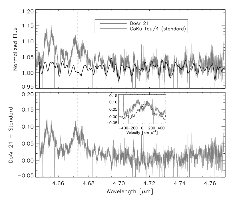
Figure 14.— Top: Spectrum of DoAr 21 (K1) observed with CRIRES (gray) and a rotationally-broadened, veiled spectrum of CoKu Tau/4 (K3) observed with NIRSPEC (black). Dotted lines mark the locations of Pf$\beta$ and Hu$\epsilon$. Bottom: Difference spectrum. Inset: Difference spectrum centered at 4.6538 $\mu$m (gray) compared with observations of H$\alpha$ from Jensen et al. (2009).

We also note that the best fit to the observed DoAr 21 spectrum requires a veiling of $\sim$ 2.6, and that the spectrum is inconsistent with zero veiling, consistent with the results of Salyk et al. (2009). Assuming the continuum flux is emitted entirely by grains at 1500 K with an opacity of 500 cm²g^-1 (appropriate for sub-micron sized grains), the mass in small grains is $\sim$10¹⁹ kg, or $\sim 10^{-4}$ M_☽. This is almost certainly a lower limit, as there is likely a range of grain sizes and a range of grain temperatures, with 1500 K being the approximate maximum temperature for solid silicates. An alternative way to explain finite veiling would be for the stellar disk to contain hotspots with featureless emission spectra. However, even in an extreme case of 10⁴ K hotspots, 54% of the stellar disk would need to be covered by hotspots to explain the observed veiling. In contrast, results from photometric variability studies (Bouvier et al., 1995) find hotspot temperatures of no more than a few hundred to a few thousand K hotter than the stellar temperatures, and $0.5-40$% disk covering fractions. Thus, DoAr 21 may retain both a gas and dust disk at small radii.

Table 1Log of Observations

Star	Date	Exp	Vdop	Std
	[yyyy mmm dd]	[s]	[km s-1]
NIRSPEC
AA Tau	2003 Nov 03	720	$-15$	HR 1620
	2004 Dec 27	780	13	HR 1620
AB Aur	2001 Jan 30	360	24	HR 1620
	2001 Aug 07	180	$-25$	HR 1620
	2002 Jan 03	240	13	HR 1620
AS 205 N	2002 Apr 21	240	$-17$	HR 6175
	2002 Jul 22	480	24	HR 5984
AS 205 S	2002 Apr 21	360	$-17$	HR 6175
BF Ori	2009 Dec 28	240	6	HR 1620
CI Tau	2008 Oct 10	480	$-24$	HR 1251
CK 4	2006 Jul 07	600	3	HR 7141
DF Tau	2005 Dec 21	240	10	HR 1620
DG Tau	2001 Oct 26	225	$-17$	HR 1177
	2005 Dec 12	120	6	HR 1620
	2005 Dec 19	720	9	HR 1620
DL Tau	2003 Nov 03	960	$-15$	HR 1620
DM Tau	2003 Nov 03	720	$-14$	HR 1620
	2006 Oct 09	1380	$-24$	HR 1251
DoAr 44	2002 Jul 22	480	22	HR 5984
	2004 Jul 23	720	23	HR 6175
	2005 Apr 26	480	$-17$	HR 6070
DO Tau	2005 Dec 18	240	8	HR 1620
	2005 Dec 20	480	9	HR 1620
DP Tau	2006 Dec 29	480	13	HR 1620
DR Tau	2002 Dec 17	480	7	HR 1620
	2005 Dec 18	240	7	HR 1620
DS Tau	2007 Dec 26	420	10	HR 1620
FS CMa	2002 Dec 17	240	$-6$	HR 1620
FT Tau	2008 Dec 10	900	5	HR 1620
FZ Tau	2008 Dec 08	480	3	HR 1620
GM Aur	2004 Dec 27	780	10	HR 1620
GQ Lup	2006 Apr 15	840	$-18$	HR 5812
GV Tau S	2008 Dec 10	630	5	HR 1620
GY 224	2006 Jul 07	420	17	HR 7141
Haro 1-1	2005 Apr 25	840	$-17$	HR 6175
	2009 Jul 13	240	19	HR 5993
	2009 Jul 13	480	20	HR 5993
Haro 1-4	2009 Jul 13	300	20	HR 5993
Haro 6-13	2008 Dec 08	480	3	HR 1620
HD 135344 B	2005 Apr 24	480	$-11$	HR 5712
	2006 Jul 06	240	20	HR 5812
HD 141569 A	2002 Apr 21	210	$-13$	HR 6175
	2008 Jul 09	480	22	HR 5685
HD 142666	2002 Jul 21	240	24	HR 5984
HD 143006	2005 Apr 26	480	$-14$	HR 6175
HD 144432 S	2002 Jul 21	480	23	HR 5984
	2005 Apr 26	480	$-15$	HR 6175
HD 150193	2002 Jul 22	480	22	HR 5984
HD 163296	2001 Aug 08	150	21	HR 6581
	2002 Apr 21	240	$-25$	HR 6378
	2002 Jul 22	480	15	HR 7141
HD 169142	2002 Jul 21	420	11	HR 6175
	2006 Jul 07	240	5	HR 7141
HD 179218	2006 Oct 10	180	23	HR 7235
HD 190073	2002 Jul 22	480	$-2$	HR 7141
	2005 Sep 22	600	22	HR 7724
HD 244604	2009 Dec 28	240	7	HR 1620
HD 35187	2009 Dec 28	420	8	HR 2714
HD 37258	2009 Dec 28	240	6	HR 1620
HD 37357	2009 Dec 28	240	6	HR 1620
HD 37411	2009 Dec 28	420	6	HR 2714
HD 37806	2009 Dec 28	240	5	HR 2714
HD 38120	2009 Dec 28	240	5	HR 2714
HD 50138	2009 Dec 28	240	$-4$	HR 2714
HD 58647	2008 Dec 08	240	$-16$	HR 1620
	2009 Dec 28	480	$-8$	HR 2714
HL Tau	2001 Oct 25	200	$-18$	HR 1380
	2002 Dec 17	240	8	HR 1620
IM Lup	2006 Jul 06	420	18	HR 5812
IRAS 03259+3105	2002 Dec 18	240	14	HR 1177
IRAS 03301+3111	2001 Oct 26	200	$-12$	HR 1177
	2002 Dec 16	720	13	HR 1177
	2002 Dec 17	360	13	HR 1177
IRAS 03445+3242	2002 Dec 16	480	11	HR 1177
	2001 Oct 26	300	$-14$	HR 1177
IRAS 04239+2436	2005 Dec 12	360	6	HR 1620
IRS 51	2002 Apr 21	300	$-19$	HR 6175
IRS 60 S	2002 Jul 21	480	22	HR 6175
LkHa 25	2006 Apr 16	480	28	HR 2714
LkHa 198	2002 Jul 22	480	$-18$	HR 7945
LkHa 220	2001 Jan 30	600	9	HR 1620
LkHa 271	2009 Dec 28	780	18	HR 1620
LkHa 326	2002 Jul 22	960	$-25$	HR 1177
	2002 Dec 16	600	13	HR 1177
LkHa 327 NE	2002 Dec 16	240	13	HR 1177
	2002 Dec 16	480	13	HR 1177
LkHa 327 SW	2002 Dec 16	240	13	HR 1177
	2002 Dec 16	480	13	HR 1177
LkHa 330	2002 Dec 16	480	11	HR 1177
	2003 Nov 02	360	$-11$	HR 1620
	2003 Nov 03	960	$-10$	HR 1177
	2004 Dec 27	480	17	HR 1177
LkHa 348	2002 Apr 21	120	-26	HR 7141
	2009 Jul 12	240	5	HR 7141
	2002 Apr 21	300	27	HR 2763
	2002 Dec 16	240	$-7$	HR 2034
	2004 Dec 27	480	$-1$	HR 2763
MWC 480	2001 Jan 30	480	24	HR 1620
	2001 Aug 08	360	$-25$	HR 1620
	2002 Dec 17	480	4	HR 1620
MWC 758	2002 Apr 21	120	24	HR 2763
	2002 Dec 16	240	0	HR 2034
MWC 1080	2002 Jul 22	480	$-16$	HR 7945
RNO 19	2005 Dec 19	900	13	HR 1177
RNO 90	2002 Jul 21	600	22	HR 5984
RNO 91	2002 Jul 21	600	22	HR 5984
	2003 Jul 10	180	18	HR 6175
ROX 43A	2002 Apr 21	300	$-19$	HR 6175
RR Tau	2005 Dec 18	180	0	HR 1620
RXJ1842.9-3532	2005 Apr 26	480	$-26$	HR 7121
RY Tau	2002 Dec 17	720	9	HR 1620
SR 4	2005 Apr 25	960	$-17$	HR 6175
SU Aur	2002 Dec 16	240	4	HR 1620
	2003 Nov 02	240	$-18$	HR 1620
	2003 Nov 03	960	$-17$	HR 1620
T Tau S	2002 Jan 03	360	18	HR 1620
	2002 Dec 16	240	9	HR 1177
	2002 Dec 17	240	9	HR 1177
	2004 Dec 27	480	15	HR 1620
T Tau N	2002 Jan 03	360	18	HR 1620
	2002 Dec 16	240	9	HR 1177
	2002 Dec 17	240	9	HR 1177
	2004 Dec 27	480	15	HR 1620
TW Hya	2001 Jan 29	1020	$-19$	HR 4494
	2001 Jan 30	1170	$-19$	HR 4494
	2002 Apr 21	570	11	HR 4313
	2002 Dec 17	1020	$-24$	HR 1620
	2004 Dec 27	300	$-24$	HR 4313
	2005 Apr 25	960	12	HR 4494
	2005 Dec 18	960	$-24$	HR 4494
UY Aur A	2006 Dec 29	420	11	HR 1620
	2007 Oct 30	420	$-18$	HR 1620
UY Aur B	2007 Oct 30	180	$-18$	HR 1620
UX Ori	2005 Dec 12	300	3	HR 1620
	2005 Dec 19	720	6	HR 1620
VSSG 1	2008 Jul 10	120	19	HR 5993
VV Ser	2001 Aug 06	600	16	HR 7141
	2003 Jul 09	1380	4	HR 7141
V1685 Cyg	2005 Sep 21	720	9	HR 7546
V1977 Cyg	2005 Sep 21	600	6	HR 7546
Wa Oph 6	2005 Apr 26	240	$-18$	HR 6175
WL 16	2002 Apr 21	240	$-19$	HR 6378
WL 22	2005 Apr 25	330	$-17$	HR 6175
WW Vul	2002 Jul 22	480	1	HR 7141
	2005 Sep 22	660	19	HR 7724
CRIRES
AA Tau	2007 Oct 13	600	$-23$	HR 1178
AS 205 N	2007 Apr 22	1200	$-16$	HR 4757
AS 209	2008 May 02	480	$-15$	HR 6084
CrA IRS 2	2007 Apr 26	480	$-26$	HR 7236
CV Cha	2009 Jan 04	1200	$-9$	HR 4467
CW Tau	2008 Dec 31	720	16	HR 2451
DF Tau	2009 Jan 02	720	16	HR 2550
DG Tau	2007 Oct 16	720	$-21$	HR 2550
DoAr 21	2008 May 01	720	$-14$	HR 7236
DoAr 24 E S	2007 Sep 03	600	29	HR 7913
DoAr 24 E N	2007 Sep 03	600	29	HR 7913
DoAr 44	2007 Sep 05	960	29	HR 6084
DR Tau	2007 Oct 11	480	$-24$	HR 3117
EC 90 N	2007 Apr 24	600	$-24$	HR 5531
EC 90 S	2007 Apr 24	600	$-24$	HR 5531
Elias 29	2008 Aug 09	360	27	HR 7235
EX Lup	2008 Apr 28	480	$-13$	HR 6084
GQ Lup	2007 Apr 22	1200	$-15$	HR 4757
Haro 1-4	2008 Apr 30	720	$-14$	HR 6074
HD 135344 B	2007 Apr 23	2400	$-11$	HR 5531
HD 142527	2008 Aug 07	360	25	HR 5984
HD 144432 S	2008 Aug 03	2880	26	HR 6508
HD 144965	2008 Apr 30	720	$-13$	HR 6084
HH 100	2007 Sep 03	600	24	HR 6508
HL Tau	2007 Oct 12	600	$-22$	HR 838
IRS 43	2008 Aug 06	960	26	HR 6175
IRS 44 E	2008 Aug 07	960	26	HR 6175
IRS 48	2008 May 03	240	$-13$	HR 6084
IRS 51	2008 Aug 03	1200	25	HR 6175
IRS 63	2007 Apr 26	600	$-17$	HR 5531
LkHa 330	2008 Dec 30	720	17	HR 1149
LLN 8	2007 Oct 12	720	$-12$	HR 3117
LLN 17	2007 Oct 14	1080	$-11$	HR 3117
RNO 91	2007 Apr 24	600	$-17$	HR 5531
RU Lup	2007 Apr 27	600	$-13$	HR 5531
S CrA A	2007 Apr 23	480	$-27$	HR 5531
S CrA B	2007 Apr 23	480	$-27$	HR 5531
Sz 68	2007 Apr 27	600	$-12$	HR 5531
T CrA	2007 Apr 24	600	$-27$	HR 5531
TW Hya	2007 Apr 22	1200	11	HR 4757
TY CrA	2007 Apr 25	600	$-26$	HR 7236
VSSG 1	2008 Aug 07	960	26	HR 6175
VV CrA S	2007 Apr 25	600	$-26$	HR 7236
VV CrA N	2007 Apr 25	600	$-26$	HR 7236
VW Cha	2009 Jan 04	720	$-8$	HR 4467
VZ Cha	2009 Jan 04	720	$-9$	HR 4467
Wa Oph 6	2008 May 02	480	$-15$	HR 6084
WL 12	2007 Sep 02	960	29	HR 5812
WL 22	2008 Aug 04	1200	26	HR 6175

Table 2Photometry

Star	M	4.5	5.8	Refs
AA Tau	6.86	6.77	6.35	THE SPECIAL CASE OF DOAR 21,THE SPECIAL CASE OF DOAR 21
AB Aur	2.70	$\cdots$	$\cdots$	THE SPECIAL CASE OF DOAR 21
AS 205 N	4.18	$\cdots$	$\cdots$	THE SPECIAL CASE OF DOAR 21
AS 205 S	5.31	$\cdots$	$\cdots$	THE SPECIAL CASE OF DOAR 21
AS 209	$\cdots$	$\cdots$	5.05	THE SPECIAL CASE OF DOAR 21
BF Ori	$\cdots$	$\cdots$	$\cdots$	$\cdots$
CI Tau	$\cdots$	6.27	5.94	THE SPECIAL CASE OF DOAR 21
CK 4	$\cdots$	7.49	7.56	THE SPECIAL CASE OF DOAR 21
CrA IRS 2	4.03	$\cdots$	$\cdots$	THE SPECIAL CASE OF DOAR 21
CV Cha	$\cdots$	$\cdots$	$\cdots$	$\cdots$
CW Tau	5.09	$\cdots$	$\cdots$	THE SPECIAL CASE OF DOAR 21
DF Tau	5.17	$\cdots$	5.28	THE SPECIAL CASE OF DOAR 21,THE SPECIAL CASE OF DOAR 21
DG Tau	4.63	$\cdots$	4.19	THE SPECIAL CASE OF DOAR 21,THE SPECIAL CASE OF DOAR 21
DL Tau	6.04	6.12	5.66	THE SPECIAL CASE OF DOAR 21,THE SPECIAL CASE OF DOAR 21
DM Tau	$\cdots$	9.19	9.25	THE SPECIAL CASE OF DOAR 21
DoAr 21	5.51	5.87	5.51	THE SPECIAL CASE OF DOAR 21,THE SPECIAL CASE OF DOAR 21
DoAr 24 E S	$\cdots$	$\cdots$	$\cdots$	$\cdots$
DoAr 24 E N	$\cdots$	$\cdots$	$\cdots$	$\cdots$
DoAr 44	$\cdots$	6.30	5.94	THE SPECIAL CASE OF DOAR 21
DO Tau	5.27	5.65	5.20	THE SPECIAL CASE OF DOAR 21,THE SPECIAL CASE OF DOAR 21
DP Tau	$\cdots$	6.91	6.37	THE SPECIAL CASE OF DOAR 21
DR Tau	4.80	$\cdots$	4.50	THE SPECIAL CASE OF DOAR 21,THE SPECIAL CASE OF DOAR 21
DS Tau	$\cdots$	6.91	6.62	THE SPECIAL CASE OF DOAR 21
EC 90 N	5.76	$\cdots$	$\cdots$	THE SPECIAL CASE OF DOAR 21
EC 90 S	4.50	$\cdots$	$\cdots$	THE SPECIAL CASE OF DOAR 21
Elias 29	2.40	$\cdots$	$\cdots$	THE SPECIAL CASE OF DOAR 21
EX Lup	3.88	$\cdots$	$\cdots$	THE SPECIAL CASE OF DOAR 21
FS CmA	$\cdots$	$\cdots$	$\cdots$	$\cdots$
FT Tau	$\cdots$	7.15	6.88	THE SPECIAL CASE OF DOAR 21
FZ Tau	$\cdots$	5.69	5.21	THE SPECIAL CASE OF DOAR 21
GM Aur	$\cdots$	7.88	7.70	THE SPECIAL CASE OF DOAR 21
GQ Lup	$\cdots$	$\cdots$	5.64	THE SPECIAL CASE OF DOAR 21
GV Tau S	$\cdots$	$\cdots$	$\cdots$	$\cdots$
GY 224	$\cdots$	6.92	6.28	THE SPECIAL CASE OF DOAR 21
Haro 1-1	8.03	$\cdots$	9.80	THE SPECIAL CASE OF DOAR 21,THE SPECIAL CASE OF DOAR 21
Haro 1-4	$\cdots$	$\cdots$	6.24	THE SPECIAL CASE OF DOAR 21
Haro 6-13	5.65	$\cdots$	$\cdots$	THE SPECIAL CASE OF DOAR 21
HD 135344 B	4.69	$\cdots$	$\cdots$	THE SPECIAL CASE OF DOAR 21
HD 141569 A	6.58	$\cdots$	$\cdots$	THE SPECIAL CASE OF DOAR 21
HD 142527	3.50	$\cdots$	$\cdots$	THE SPECIAL CASE OF DOAR 21
HD 142666	4.69	$\cdots$	$\cdots$	THE SPECIAL CASE OF DOAR 21
HD 143006	5.34	$\cdots$	$\cdots$	THE SPECIAL CASE OF DOAR 21
HD 144432 S	4.90	$\cdots$	$\cdots$	THE SPECIAL CASE OF DOAR 21
HD 144965	$\cdots$	$\cdots$	$\cdots$	$\cdots$
HD 150193	3.93	$\cdots$	$\cdots$	THE SPECIAL CASE OF DOAR 21
HD 163296	3.14	$\cdots$	$\cdots$	THE SPECIAL CASE OF DOAR 21
HD 169142	5.57	$\cdots$	$\cdots$	THE SPECIAL CASE OF DOAR 21
HD 179218	4.18	$\cdots$	$\cdots$	THE SPECIAL CASE OF DOAR 21
HD 190073	$\cdots$	$\cdots$	$\cdots$	$\cdots$
HD 244604	5.37	$\cdots$	$\cdots$	THE SPECIAL CASE OF DOAR 21
HD 35187	$\cdots$	$\cdots$	$\cdots$	$\cdots$
HD 37258	$\cdots$	$\cdots$	$\cdots$	$\cdots$
HD 37357	$\cdots$	$\cdots$	$\cdots$	$\cdots$
HD 37411	5.81	$\cdots$	$\cdots$	$\cdots$
HD 37806	3.79	$\cdots$	$\cdots$	THE SPECIAL CASE OF DOAR 21
HD 38120	$\cdots$	$\cdots$	$\cdots$	$\cdots$
HD 50138	$\cdots$	$\cdots$	$\cdots$	$\cdots$
HD 58647	3.50	$\cdots$	$\cdots$	THE SPECIAL CASE OF DOAR 21
HH 100	$\cdots$	$\cdots$	$\cdots$	$\cdots$
HL Tau	4.09	$\cdots$	$\cdots$	THE SPECIAL CASE OF DOAR 21
IM Lup	6.55	7.28	6.43	THE SPECIAL CASE OF DOAR 21,THE SPECIAL CASE OF DOAR 21
IRAS 03259+3105	$\cdots$	6.74	4.05	THE SPECIAL CASE OF DOAR 21
IRAS 03301+3111	$\cdots$	6.53	5.65	THE SPECIAL CASE OF DOAR 21
IRAS 03445+3242	$\cdots$	5.86	4.80	THE SPECIAL CASE OF DOAR 21
IRAS 04239+2436	$\cdots$	6.32	5.38	THE SPECIAL CASE OF DOAR 21
IRS 43	$\cdots$	5.00	4.01	THE SPECIAL CASE OF DOAR 21
IRS 44 E	5.21	$\cdots$	$\cdots$	THE SPECIAL CASE OF DOAR 21
IRS 48	$\cdots$	5.12	3.64	THE SPECIAL CASE OF DOAR 21
IRS 51	$\cdots$	5.73	5.17	THE SPECIAL CASE OF DOAR 21
IRS 60 S	$\cdots$	6.10	5.45	THE SPECIAL CASE OF DOAR 21
IRS 63	5.58	$\cdots$	$\cdots$	THE SPECIAL CASE OF DOAR 21
LkHa 25	6.91	$\cdots$	$\cdots$	THE SPECIAL CASE OF DOAR 21
LkHa 198	$\cdots$	$\cdots$	$\cdots$	$\cdots$
LkHa 220	7.00	$\cdots$	$\cdots$	THE SPECIAL CASE OF DOAR 21
LkHa 271	$\cdots$	8.22	8.02	THE SPECIAL CASE OF DOAR 21
LkHa 326	$\cdots$	6.97	6.49	THE SPECIAL CASE OF DOAR 21
LkHa 327 NE	$\cdots$	$\cdots$	$\cdots$	$\cdots$
LkHa 327 SW	$\cdots$	$\cdots$	$\cdots$	$\cdots$
LkHa 330	$\cdots$	5.77	5.48	THE SPECIAL CASE OF DOAR 21
LkHa 348	$\cdots$	$\cdots$	$\cdots$	$\cdots$
LLN 8	4.01	$\cdots$	$\cdots$	THE SPECIAL CASE OF DOAR 21
LLN 17	4.70	$\cdots$	$\cdots$	THE SPECIAL CASE OF DOAR 21
MCW 442	3.50	$\cdots$	$\cdots$	$\cdots$
MWC 480	$\cdots$	$\cdots$	$\cdots$	$\cdots$
MWC 758	4.47	$\cdots$	$\cdots$	THE SPECIAL CASE OF DOAR 21
MWC 1080	2.40	$\cdots$	$\cdots$	THE SPECIAL CASE OF DOAR 21
RNO 19	$\cdots$	6.78	6.22	THE SPECIAL CASE OF DOAR 21
RNO 90	$\cdots$	$\cdots$	4.43	THE SPECIAL CASE OF DOAR 21
RNO 91	$\cdots$	$\cdots$	$\cdots$	$\cdots$
ROX 43A	$\cdots$	5.88	5.29	THE SPECIAL CASE OF DOAR 21
RR Tau	5.50	$\cdots$	$\cdots$	THE SPECIAL CASE OF DOAR 21
RU Lup	5.38	$\cdots$	5.12	THE SPECIAL CASE OF DOAR 21,THE SPECIAL CASE OF DOAR 21
RXJ1842.9-3532	$\cdots$	7.30	$\cdots$	THE SPECIAL CASE OF DOAR 21
RY Tau	3.38	$\cdots$	$\cdots$	THE SPECIAL CASE OF DOAR 21
S CrA A	4.15	$\cdots$	$\cdots$	THE SPECIAL CASE OF DOAR 21
S CrA B	5.33	$\cdots$	$\cdots$	THE SPECIAL CASE OF DOAR 21
SR 4	6.90	6.19	5.86	THE SPECIAL CASE OF DOAR 21,THE SPECIAL CASE OF DOAR 21
SU Aur	4.26	$\cdots$	4.64	THE SPECIAL CASE OF DOAR 21,THE SPECIAL CASE OF DOAR 21
Sz 68	$\cdots$	5.25	4.60	THE SPECIAL CASE OF DOAR 21
T CrA	5.18	$\cdots$	$\cdots$	THE SPECIAL CASE OF DOAR 21
T Tau S	$\cdots$	$\cdots$	$\cdots$	$\cdots$
T Tau N	$\cdots$	$\cdots$	$\cdots$	$\cdots$
TW Hya	$\cdots$	7.07	6.93	THE SPECIAL CASE OF DOAR 21
TY CrA	5.83	$\cdots$	$\cdots$	THE SPECIAL CASE OF DOAR 21
UY Aur A	$\cdots$	$\cdots$	$\cdots$	$\cdots$
UY Aur B	$\cdots$	$\cdots$	$\cdots$	$\cdots$
UX Ori	5.32	$\cdots$	$\cdots$	THE SPECIAL CASE OF DOAR 21
VSSG 1	$\cdots$	5.62	5.20	THE SPECIAL CASE OF DOAR 21
VV CrA S	$\cdots$	$\cdots$	$\cdots$	$\cdots$
VV CrA N	$\cdots$	$\cdots$	$\cdots$	$\cdots$
VV Ser	4.40	4.63	3.83	THE SPECIAL CASE OF DOAR 21,THE SPECIAL CASE OF DOAR 21
VW Cha	$\cdots$	$\cdots$	$\cdots$	$\cdots$
VZ Cha	$\cdots$	$\cdots$	$\cdots$	$\cdots$
V1685 Cyg	$\cdots$	$\cdots$	$\cdots$	$\cdots$
V1977 Cyg	$\cdots$	$\cdots$	$\cdots$	$\cdots$
Wa Oph 6	$\cdots$	5.72	5.79	THE SPECIAL CASE OF DOAR 21
WL 12	5.76	$\cdots$	$\cdots$	THE SPECIAL CASE OF DOAR 21
WL 16	$\cdots$	4.90	3.41	THE SPECIAL CASE OF DOAR 21
WL 22	$\cdots$	6.42	5.79	THE SPECIAL CASE OF DOAR 21
WW Vul	$\cdots$	$\cdots$	$\cdots$	$\cdots$

References. — (1) Bouvier et al. 1992 (2) Carpenter et al. 2008 (3) Cieza et al. 2007 (4) Ducati et al. 2002 (5) Evans et al. 2003 (6) Evans et al. 2009 (7) Goto et al. 2011 (8) Hartmann et al. 2005 (9) Herczeg et al. 2011 (10) Hillenbrand et al. 1992 (11) Hughes et al. 1994 (12) Kenyon & Hartmann 1995 (13) Lada et al. 2006 (14) Liseau et al. 1992 (15) Luhman et al. 2006 (16) Malfait et al. 1998 (17) McCabe et al. 2006 (18) Merín et al. 2004 (19) Merín et al. 2008 (20) Padgett et al. 2006 (21) Padgett et al. 2007 (22) Pinte et al. 2008 (23) Rebull et al. 2010 (24) Robitaille et al. 2007 (25) Schegerer et al. 2009 (26) Wright et al. 2010

Table 3Stellar and disk parameters

Star	dist	SpT	$T_{\star}$	$L_{\star}$	$R_{\star}$	$M_{\star}$	$A_{V}$	Refs	Stage	Ref	Inst.
AA Tau	140	K7	4060	0.71	1.74	0.53	0.74	THE SPECIAL CASE OF DOAR 21	II	$\cdots$	N,C
AB Aur	140	A0	9840	48	$\cdots$	2.40	0.5	THE SPECIAL CASE OF DOAR 21	II	$\cdots$	N
AS 205 N	160	K5	4450	7.1	$\cdots$	1.50	2.9	THE SPECIAL CASE OF DOAR 21	II	$\cdots$	N,C
AS 205 S	160	M3	3450	2.19	$\cdots$	0.30	2.1	THE SPECIAL CASE OF DOAR 21	II	$\cdots$	N
AS 209	160	K5	4395	2.5	2.40	1.40	1.15	THE SPECIAL CASE OF DOAR 21	II	$\cdots$	C
BF Ori	400	A5-F6	$\cdots$	27	2.70	2.10	2.4	THE SPECIAL CASE OF DOAR 21,THE SPECIAL CASE OF DOAR 21	II	$\cdots$	N
CI Tau	140	K7	4060	0.84	$\cdots$	0.77	1.8	THE SPECIAL CASE OF DOAR 21	II	$\cdots$	N
CK 4	260	K3	4730	$\cdots$	$\cdots$	$\cdots$	12.8	THE SPECIAL CASE OF DOAR 21,THE SPECIAL CASE OF DOAR 21	II	THE SPECIAL CASE OF DOAR 21	N
CrA IRS 2	130	K2	4900	$\cdots$	$\cdots$	$\cdots$	20	THE SPECIAL CASE OF DOAR 21	I	THE SPECIAL CASE OF DOAR 21	C
CV Cha	215	G8	5451	8.0	3.20	2.10	1.67	THE SPECIAL CASE OF DOAR 21	II	$\cdots$	C
CW Tau	140	K3	4730	0.76	$\cdots$	1.06	2.21	THE SPECIAL CASE OF DOAR 21	II	$\cdots$	C
DF Tau	140	M0.5	3470	1.97	3.37	0.27	0.45	THE SPECIAL CASE OF DOAR 21,THE SPECIAL CASE OF DOAR 21,THE SPECIAL CASE OF DOAR 21	II	$\cdots$	N,C
DG Tau	140	K6	4200	0.28	1.00	0.85	1.3	THE SPECIAL CASE OF DOAR 21,THE SPECIAL CASE OF DOAR 21	II	$\cdots$	N,C
DL Tau	140	K7	4060	1.16	$\cdots$	0.76	2.0	THE SPECIAL CASE OF DOAR 21,THE SPECIAL CASE OF DOAR 21	II	$\cdots$	N
DM Tau	140	M1	3705	0.32	$\cdots$	0.62	1.1	THE SPECIAL CASE OF DOAR 21,THE SPECIAL CASE OF DOAR 21,THE SPECIAL CASE OF DOAR 21	IIt	$\cdots$	N
DoAr 21	122	K1	5080	11.7	$\cdots$	1.80	6.0	THE SPECIAL CASE OF DOAR 21,THE SPECIAL CASE OF DOAR 21,THE SPECIAL CASE OF DOAR 21	II	$\cdots$	C
DoAr 24 E S	120	K0	5250	8.78	$\cdots$	0.47	5.7	THE SPECIAL CASE OF DOAR 21,THE SPECIAL CASE OF DOAR 21	II	$\cdots$	C
DoAr 24 E N	120	$\cdots$	$\cdots$	$\cdots$	$\cdots$	$\cdots$	5.7	$\cdots$	II	$\cdots$	C
DoAr 44	120	K3	4730	1.4	1.75	1.30	2.2	THE SPECIAL CASE OF DOAR 21	IIt	$\cdots$	N,C
DO Tau	140	M0	3850	1.0	2.25	0.37	2.3	THE SPECIAL CASE OF DOAR 21	II	$\cdots$	N
DP Tau	140	M0	3850	0.18	$\cdots$	0.57	0.6	THE SPECIAL CASE OF DOAR 21,THE SPECIAL CASE OF DOAR 21,THE SPECIAL CASE OF DOAR 21	II	$\cdots$	N
DR Tau	140	K7	4060	1.7	$\cdots$	0.40	1.7	THE SPECIAL CASE OF DOAR 21,THE SPECIAL CASE OF DOAR 21	II	$\cdots$	N,C
DS Tau	140	K5	4350	0.57	1.36	0.87	0.34	THE SPECIAL CASE OF DOAR 21	II	$\cdots$	N
EC 90 N	415	M5	3270	$\cdots$	$\cdots$	$\cdots$	4.0	THE SPECIAL CASE OF DOAR 21	I	THE SPECIAL CASE OF DOAR 21	C
EC 90 S	415	G1	5900	$\cdots$	$\cdots$	$\cdots$	30	THE SPECIAL CASE OF DOAR 21	I	THE SPECIAL CASE OF DOAR 21	C
Elias 29	120	$\cdots$	$\cdots$	$\cdots$	$\cdots$	$\cdots$	9.8	THE SPECIAL CASE OF DOAR 21	I	THE SPECIAL CASE OF DOAR 21,THE SPECIAL CASE OF DOAR 21	C
EX Lup	140	M0	3802	0.39	$\cdots$	$\cdots$	0	THE SPECIAL CASE OF DOAR 21	II	$\cdots$	C
FS CmA	500	$\cdots$	21878	3162	$\cdots$	$\cdots$	1.0	THE SPECIAL CASE OF DOAR 21,THE SPECIAL CASE OF DOAR 21	II	$\cdots$	N
FT Tau	140	Cont	3890	$\cdots$	$\cdots$	$\cdots$	0	THE SPECIAL CASE OF DOAR 21,THE SPECIAL CASE OF DOAR 21,THE SPECIAL CASE OF DOAR 21	II	$\cdots$	N
FZ Tau	140	M0	3918	0.51	$\cdots$	0.70	2.72	THE SPECIAL CASE OF DOAR 21	II	$\cdots$	N
GM Aur	140	K7	4060	0.74	1.78	0.52	0.31	THE SPECIAL CASE OF DOAR 21	IIt	$\cdots$	N
GQ Lup	100	K7	4060	0.8	$\cdots$	0.80	0.5	THE SPECIAL CASE OF DOAR 21,THE SPECIAL CASE OF DOAR 21	II	$\cdots$	N,C
GV Tau S	140	K4	4500	4.9	$\cdots$	$\cdots$	30	THE SPECIAL CASE OF DOAR 21,THE SPECIAL CASE OF DOAR 21	I	$\cdots$	N
GY 224	120	M4	4635	3.7	$\cdots$	0.91	34.2	THE SPECIAL CASE OF DOAR 21,THE SPECIAL CASE OF DOAR 21	I	THE SPECIAL CASE OF DOAR 21	N
Haro 1-1	120	K5-K7	4205	$\cdots$	$\cdots$	$\cdots$	1.67	THE SPECIAL CASE OF DOAR 21,THE SPECIAL CASE OF DOAR 21	II	$\cdots$	N
Haro 1-4	120	K4-K6	4350	$\cdots$	$\cdots$	$\cdots$	3.8	THE SPECIAL CASE OF DOAR 21,THE SPECIAL CASE OF DOAR 21	II	$\cdots$	N,C
Haro 6-13	140	M0	3800	2.11	$\cdots$	0.52	11.9	THE SPECIAL CASE OF DOAR 21	II	$\cdots$	N
HD 135344 B	84	F3	6590	8.0	$\cdots$	1.50	0.3	THE SPECIAL CASE OF DOAR 21	IIt	$\cdots$	N,C
HD 141569 A	99	B9.5	9550	22.9	1.80	2.20	0.1	THE SPECIAL CASE OF DOAR 21,THE SPECIAL CASE OF DOAR 21	IIt	$\cdots$	N
HD 142527	200	F6	6270	69	$\cdots$	3.50	0.7	THE SPECIAL CASE OF DOAR 21	II	$\cdots$	C
HD 142666	145	A8	7590	17	2.40	2.00	0.8	THE SPECIAL CASE OF DOAR 21,THE SPECIAL CASE OF DOAR 21	II	$\cdots$	N
HD 143006	145	G5	5884	2.5	$\cdots$	$\cdots$	1.63	THE SPECIAL CASE OF DOAR 21,THE SPECIAL CASE OF DOAR 21,THE SPECIAL CASE OF DOAR 21	II	$\cdots$	N
HD 144432 S	145	A9	7410	14.8	2.30	2.00	0.2	THE SPECIAL CASE OF DOAR 21,THE SPECIAL CASE OF DOAR 21	II	$\cdots$	N,C
HD 144965	190	B5	$\cdots$	$\cdots$	$\cdots$	$\cdots$	0	THE SPECIAL CASE OF DOAR 21,THE SPECIAL CASE OF DOAR 21,THE SPECIAL CASE OF DOAR 21	II	$\cdots$	C
HD 150193	203	A1	8970	36.1	2.50	2.20	1.5	THE SPECIAL CASE OF DOAR 21,THE SPECIAL CASE OF DOAR 21	II	$\cdots$	N
HD 163296	122	A1	9450	36	$\cdots$	2.30	0.3	THE SPECIAL CASE OF DOAR 21	II	$\cdots$	N
HD 169142	145	A5	8260	15	$\cdots$	1.80	0.3	THE SPECIAL CASE OF DOAR 21	II	$\cdots$	N
HD 179218	240	B9	10600	500	$\cdots$	4.00	1.8	THE SPECIAL CASE OF DOAR 21	II	$\cdots$	N
HD 190073	767	A2	9500	471	8.00	5.10	0.5	THE SPECIAL CASE OF DOAR 21,THE SPECIAL CASE OF DOAR 21,THE SPECIAL CASE OF DOAR 21	II	$\cdots$	N
HD 244604	336	A0	9549	97.7	$\cdots$	3.05	1.69	THE SPECIAL CASE OF DOAR 21,THE SPECIAL CASE OF DOAR 21,THE SPECIAL CASE OF DOAR 21	II	$\cdots$	N
HD 35187	150	A2	9120	27	$\cdots$	2.30	0.65	THE SPECIAL CASE OF DOAR 21	II	$\cdots$	N
HD 37258	510	A2	8970	$\cdots$	$\cdots$	$\cdots$	0.3	THE SPECIAL CASE OF DOAR 21,THE SPECIAL CASE OF DOAR 21,THE SPECIAL CASE OF DOAR 21	II	$\cdots$	N
HD 37357	240	A2	10495	29.5	$\cdots$	2.40	0.35	THE SPECIAL CASE OF DOAR 21,THE SPECIAL CASE OF DOAR 21	II	$\cdots$	N
HD 37411	510	B9	10500	$\cdots$	$\cdots$	$\cdots$	0.52	THE SPECIAL CASE OF DOAR 21,THE SPECIAL CASE OF DOAR 21,THE SPECIAL CASE OF DOAR 21	II	$\cdots$	N
HD 37806	470	B9	8912	138	$\cdots$	3.58	0	THE SPECIAL CASE OF DOAR 21,THE SPECIAL CASE OF DOAR 21,THE SPECIAL CASE OF DOAR 21	II	$\cdots$	N
HD 38120	460	B9	10471	123	$\cdots$	3.12	0.67	THE SPECIAL CASE OF DOAR 21,THE SPECIAL CASE OF DOAR 21,THE SPECIAL CASE OF DOAR 21	II	$\cdots$	N
HD 50138	500	B6	1148	$\cdots$	$\cdots$	$\cdots$	0.2	THE SPECIAL CASE OF DOAR 21,THE SPECIAL CASE OF DOAR 21,THE SPECIAL CASE OF DOAR 21	II	$\cdots$	N
HD 58647	543	B9	10500	911	9.10	6.00	1.0	THE SPECIAL CASE OF DOAR 21,THE SPECIAL CASE OF DOAR 21,THE SPECIAL CASE OF DOAR 21	II	$\cdots$	N
HH 100	130	K7	4060	3.1	3.60	0.40	30	THE SPECIAL CASE OF DOAR 21,THE SPECIAL CASE OF DOAR 21	I	THE SPECIAL CASE OF DOAR 21	C
HL Tau	140	K5	4350	0.9	$\cdots$	0.55	3.2	THE SPECIAL CASE OF DOAR 21,THE SPECIAL CASE OF DOAR 21	I	THE SPECIAL CASE OF DOAR 21	N,C
IM Lup	140	M0	3918	1.3	$\cdots$	$\cdots$	0.98	THE SPECIAL CASE OF DOAR 21,THE SPECIAL CASE OF DOAR 21,THE SPECIAL CASE OF DOAR 21	II	$\cdots$	N
IRAS 03259+3105	250	$\cdots$	$\cdots$	$\cdots$	$\cdots$	$\cdots$	5.9	THE SPECIAL CASE OF DOAR 21	I	THE SPECIAL CASE OF DOAR 21	N
IRAS 03301+3111	250	$\cdots$	$\cdots$	$\cdots$	$\cdots$	$\cdots$	$\cdots$	$\cdots$	II	$\cdots$	N
IRAS 03445+3242	350	$\cdots$	5750	9.40	$\cdots$	$\cdots$	30	THE SPECIAL CASE OF DOAR 21	I	THE SPECIAL CASE OF DOAR 21	N
IRAS 04239+2436	140	$\cdots$	$\cdots$	0.15	$\cdots$	$\cdots$	33	THE SPECIAL CASE OF DOAR 21,THE SPECIAL CASE OF DOAR 21	I	$\cdots$	N
IRS 43	120	K5	4400	$\cdots$	$\cdots$	$\cdots$	9.8	THE SPECIAL CASE OF DOAR 21	I	THE SPECIAL CASE OF DOAR 21,THE SPECIAL CASE OF DOAR 21	C
IRS 44 E	120	K5	4400	$\cdots$	$\cdots$	$\cdots$	9.8	THE SPECIAL CASE OF DOAR 21	I	THE SPECIAL CASE OF DOAR 21	C
IRS 48	120	A0	9000	14.3	$\cdots$	2.00	11.5	THE SPECIAL CASE OF DOAR 21	IIt	$\cdots$	C
IRS 51	120	K6	5200	1.1	$\cdots$	$\cdots$	37.6	THE SPECIAL CASE OF DOAR 21,THE SPECIAL CASE OF DOAR 21,THE SPECIAL CASE OF DOAR 21	I	$\cdots$	N,C
IRS 60 S	120	K2	$\cdots$	$\cdots$	$\cdots$	$\cdots$	9.0	THE SPECIAL CASE OF DOAR 21	II	$\cdots$	N
IRS 63	120	$\cdots$	$\cdots$	$\cdots$	$\cdots$	$\cdots$	9.8	THE SPECIAL CASE OF DOAR 21	I	THE SPECIAL CASE OF DOAR 21	C
LkHa 25	800	A0	$\cdots$	$\cdots$	$\cdots$	$\cdots$	0.65	THE SPECIAL CASE OF DOAR 21,THE SPECIAL CASE OF DOAR 21	II	$\cdots$	N
LkHa 198	600	A5	$\cdots$	$\cdots$	$\cdots$	$\cdots$	4.5	THE SPECIAL CASE OF DOAR 21,THE SPECIAL CASE OF DOAR 21	II	$\cdots$	N
LkHa 220	1050	$\cdots$	$\cdots$	$\cdots$	$\cdots$	$\cdots$	$\cdots$	THE SPECIAL CASE OF DOAR 21	II	$\cdots$	N
LkHa 271	250	K3-K5	$\cdots$	$\cdots$	$\cdots$	$\cdots$	0.9	THE SPECIAL CASE OF DOAR 21,THE SPECIAL CASE OF DOAR 21	II	$\cdots$	N
LkHa 326	250	G-M0	$\cdots$	$\cdots$	$\cdots$	$\cdots$	$\cdots$	THE SPECIAL CASE OF DOAR 21	II	$\cdots$	N
LkHa 327 NE	250	$\cdots$	$\cdots$	$\cdots$	$\cdots$	$\cdots$	3.83	THE SPECIAL CASE OF DOAR 21,THE SPECIAL CASE OF DOAR 21	II	$\cdots$	N
LkHa 327 SW	250	$\cdots$	$\cdots$	$\cdots$	$\cdots$	$\cdots$	3.83	THE SPECIAL CASE OF DOAR 21,THE SPECIAL CASE OF DOAR 21	II	$\cdots$	N
LkHa 330	250	G3	5800	16	$\cdots$	2.50	1.8	THE SPECIAL CASE OF DOAR 21,THE SPECIAL CASE OF DOAR 21	IIt	$\cdots$	N,C
LkHa 348	260	$\cdots$	$\cdots$	$\cdots$	$\cdots$	$\cdots$	$\cdots$	THE SPECIAL CASE OF DOAR 21	II	$\cdots$	N
LLN 8	400	$\cdots$	$\cdots$	642	$\cdots$	5.00	20	THE SPECIAL CASE OF DOAR 21,THE SPECIAL CASE OF DOAR 21	I	$\cdots$	C
LLN 17	700	$\cdots$	$\cdots$	$\cdots$	$\cdots$	$\cdots$	20	THE SPECIAL CASE OF DOAR 21,THE SPECIAL CASE OF DOAR 21	I	$\cdots$	C
MCW 442	800	B6	14125	1550	$\cdots$	$\cdots$	1.2	THE SPECIAL CASE OF DOAR 21	II	$\cdots$	N
MWC 480	137	A5	8200	21.9	$\cdots$	1.97	0.33	THE SPECIAL CASE OF DOAR 21,THE SPECIAL CASE OF DOAR 21,THE SPECIAL CASE OF DOAR 21	II	$\cdots$	N
MWC 758	204	A3	8130	30	$\cdots$	2.00	0.66	THE SPECIAL CASE OF DOAR 21,THE SPECIAL CASE OF DOAR 21,THE SPECIAL CASE OF DOAR 21,THE SPECIAL CASE OF DOAR 21	II	$\cdots$	N
MWC 1080	2200	B0	30200	5750	$\cdots$	$\cdots$	8.4	THE SPECIAL CASE OF DOAR 21,THE SPECIAL CASE OF DOAR 21	II	$\cdots$	N
RNO 19	250	$\cdots$	$\cdots$	$\cdots$	$\cdots$	$\cdots$	3.9	THE SPECIAL CASE OF DOAR 21	II	$\cdots$	N
RNO 90	120	G5	5662	5.7	$\cdots$	1.60	$\cdots$	THE SPECIAL CASE OF DOAR 21,THE SPECIAL CASE OF DOAR 21,THE SPECIAL CASE OF DOAR 21	II	$\cdots$	N
RNO 91	120	$\cdots$	$\cdots$	$\cdots$	$\cdots$	$\cdots$	9.0	THE SPECIAL CASE OF DOAR 21	I	$\cdots$	N,C
ROX 43A	120	G0	6030	$\cdots$	$\cdots$	$\cdots$	3.5	THE SPECIAL CASE OF DOAR 21	II	$\cdots$	N
RR Tau	2103	A0	10000	781	9.30	5.80	1.1	THE SPECIAL CASE OF DOAR 21,THE SPECIAL CASE OF DOAR 21	II	$\cdots$	N
RU Lup	140	K7	4060	0.42	1.30	1.00	0.1	THE SPECIAL CASE OF DOAR 21	II	$\cdots$	C
RXJ1842.9-3532	140	K2	4995	1.12	$\cdots$	$\cdots$	1.03	THE SPECIAL CASE OF DOAR 21	II	$\cdots$	N
RY Tau	140	G1	5945	9.6	2.90	2.00	2.2	THE SPECIAL CASE OF DOAR 21	II	$\cdots$	N
S CrA A	130	K3	4800	2.29	$\cdots$	1.50	1.0	THE SPECIAL CASE OF DOAR 21	II	$\cdots$	C
S CrA B	130	M0	3800	0.76	$\cdots$	0.60	1.0	THE SPECIAL CASE OF DOAR 21	II	$\cdots$	C
SR 4	120	K6	4197	1.5	$\cdots$	0.52	1.9	THE SPECIAL CASE OF DOAR 21,THE SPECIAL CASE OF DOAR 21,THE SPECIAL CASE OF DOAR 21	II	$\cdots$	N
SU Aur	140	G1	5945	7.80	2.60	1.70	0.9	THE SPECIAL CASE OF DOAR 21	II	$\cdots$	N
Sz 68	159	K2	4900	14.49	$\cdots$	2.50	4.0	THE SPECIAL CASE OF DOAR 21	II	$\cdots$	C
T CrA	130	F0	7244	7.90	$\cdots$	$\cdots$	2.1	THE SPECIAL CASE OF DOAR 21,THE SPECIAL CASE OF DOAR 21,THE SPECIAL CASE OF DOAR 21	II	$\cdots$	C
T Tau S	140	$\cdots$	$\cdots$	$\cdots$	$\cdots$	2.50	35	THE SPECIAL CASE OF DOAR 21	II	$\cdots$	N
T Tau N	140	K0	5248	7.3	$\cdots$	2.11	1.46	THE SPECIAL CASE OF DOAR 21	II	$\cdots$	N
TW Hya	56	K7	4060	0.17	0.83	0.77	0	THE SPECIAL CASE OF DOAR 21,THE SPECIAL CASE OF DOAR 21	IIt	$\cdots$	N,C
TY CrA	130	B9	$\cdots$	$\cdots$	$\cdots$	$\cdots$	1.75	THE SPECIAL CASE OF DOAR 21,THE SPECIAL CASE OF DOAR 21	II	$\cdots$	C
UY Aur A	140	$\cdots$	$\cdots$	$\cdots$	$\cdots$	$\cdots$	2.1	THE SPECIAL CASE OF DOAR 21	II	$\cdots$	N
UY Aur B	140	$\cdots$	$\cdots$	$\cdots$	$\cdots$	$\cdots$	2.1	THE SPECIAL CASE OF DOAR 21	II	$\cdots$	N
UX Ori	450	A3	8670	39	$\cdots$	2.30	0.3	THE SPECIAL CASE OF DOAR 21	II	$\cdots$	N
VSSG 1	120	M0	3890	1.5	$\cdots$	0.52	0.97	THE SPECIAL CASE OF DOAR 21,THE SPECIAL CASE OF DOAR 21,THE SPECIAL CASE OF DOAR 21	II	$\cdots$	N,C
VV CrA S	130	K1	$\cdots$	$\cdots$	$\cdots$	$\cdots$	2.4	THE SPECIAL CASE OF DOAR 21,THE SPECIAL CASE OF DOAR 21	II	$\cdots$	C
VV CrA N	130	K1	$\cdots$	$\cdots$	$\cdots$	$\cdots$	2.4	THE SPECIAL CASE OF DOAR 21,THE SPECIAL CASE OF DOAR 21	II	$\cdots$	C
VV Ser	260	B9	10600	85	$\cdots$	3.10	3.1	THE SPECIAL CASE OF DOAR 21	II	$\cdots$	N
VW Cha	150	K5	$\cdots$	3.37	2.75	0.60	2.39	THE SPECIAL CASE OF DOAR 21,THE SPECIAL CASE OF DOAR 21	II	$\cdots$	C
VZ Cha	150	K7	4060	0.46	1.30	0.78	0.47	THE SPECIAL CASE OF DOAR 21,THE SPECIAL CASE OF DOAR 21	II	$\cdots$	C
V1685 Cyg	1000	$\cdots$	$\cdots$	$\cdots$	$\cdots$	$\cdots$	3.16	THE SPECIAL CASE OF DOAR 21,THE SPECIAL CASE OF DOAR 21	II	$\cdots$	N
V1977 Cyg	826	B8	11000	207	4.00	3.50	1.74	THE SPECIAL CASE OF DOAR 21,THE SPECIAL CASE OF DOAR 21,THE SPECIAL CASE OF DOAR 21	II	$\cdots$	N
Wa Oph 6	120	K	$\cdots$	0.67	$\cdots$	$\cdots$	3.5	THE SPECIAL CASE OF DOAR 21,THE SPECIAL CASE OF DOAR 21,THE SPECIAL CASE OF DOAR 21	II	$\cdots$	N,C
WL 12	120	K7	4000	$\cdots$	$\cdots$	$\cdots$	9.8	THE SPECIAL CASE OF DOAR 21	I	THE SPECIAL CASE OF DOAR 21	C
WL 16	120	K5	4467	4.57	$\cdots$	1.02	$\cdots$	THE SPECIAL CASE OF DOAR 21	II	$\cdots$	N
WL 22	830	$\cdots$	$\cdots$	$\cdots$	$\cdots$	$\cdots$	9.8	THE SPECIAL CASE OF DOAR 21	I	THE SPECIAL CASE OF DOAR 21	N,C
WW Vul	696	A3	8970	50	2.90	2.50	1.0	THE SPECIAL CASE OF DOAR 21,THE SPECIAL CASE OF DOAR 21	II	$\cdots$	N

References. — (1) Acke et al. 2005 (2) Andrews & Williams 2007 (3) Andrews et al. 2011 (4) Barsony et al. 2005 (5) Basri & Batalha 1990 (6) Beckwith et al. 1990 (7) Blondel et al. 2006 (8) Boersma et al. 2008 (9) Bontemps et al. 2001 (10) Boogert et al. 2002 (11) Borges Fernandes et al. 2009 (12) Bouvier & Appenzeller 1992 (13) Briceño et al. 2002 (14) Brown et al. 1995 (15) Brown et al. 2007 (16) Brown et al. 2012 (17) Calvet et al. 2004 (18) Caratti o Garatti et al. 2004 (19) Chini 1981 (20) Cohen & Kuhi 1979 (21) Correia et al. 2006 (22) de Lara et al. 1991 (23) Doppmann et al. 2003 (24) Doppmann et al. 2005 (25) Duchene et al. 2004 (26) Dunkin & Crawford 1998 (27) Evans et al. 2009 (28) Feigelson et al. 1993 (29) Friedemann et al. 1993 (30) Furlan et al. 2006 (31) Furlan et al. 2009 (32) Garcia-Lopez et al. 2006 (33) Ghez, Neugebauer & Matthews 1993 (34) Gras-Velázquez & Ray 2005 (35) Greene & Meyer 1995 (36) Gredel et al. 1997 (37) Guenther et al. 2007 (38) Gullbring et al. 1998 (39) Hartigan & Kenyon 2003 (40) Hartmann et al. 1998 (41) Herbst & Warner 1981 (42) Herczeg et al. 2004 (43) Herczeg et al. 2008 (44) Herczeg et al. 2011 (45) Hernández et al. 2004 (46) Hernández et al. 2005 (47) Heyer et al. 1990 (48) Hillenbrand et al. 2008 (49) Hodapp 1994 (50) Hughes et al. 1994 (51) Jensen et al. 2009 (52) Johns-Krull et al. 2000 (53) Johns-Krull & Gafford 2002 (54) Keller et al. 2008 (55) Kenyon & Hartmann 1995 (56) Kessler-Silacci et al. 2006 (57) K ohler et al. 2008 (58) Koresko et al. 1997 (59) Lada et al. 2006 (60) Lahuis et al. 2007 (61) Levreault 1985 (62) Liseau et al. 1992 (63) Loinard et al. 2008 (64) Luhman & Rieke 1999 (65) Malfait et al. 1998 (66) Mannings & Sargent 2000 (67) Manoj et al. 2006 (68) Massi et al. 2006 (69) Mendigutía et al. 2011 (70) Miroshnichenko 2007 (71) Monnier et al. 2005 (72) Montesinos et al. 2009 (73) Mora et al. 2001 (74) Myers et al. 1987 (75) Natta et al. 2006 (76) Neckel et al. 1980 (77) Nisini et al. 2005 (78) Pascucci et al. 2007 (79) Perryman et al. 1997 (80) Pontoppidan et al. 2007 (81) Prato et al. 2003 (82) Prato et al. 2009 (83) Rice et al. 2006 (84) Seperuelo Duarte et al. 2008 (85) Shevchenko & Herbst 1998 (86) Shevchenko et al. 1999 (87) Simon et al. 1992 (88) Steele et al. 1999 (89) Stelzer et al. 2009 (90) Straizys et al. 1996 (91) Strom et al. 1972 (92) Testi et al. 1998 (93) Thompson et al. 1998 (94) Valenti et al. 1993 (95) Valenti et al. 2003 (96) van den Ancker et al. 1998 (97) van Boekel et al. 2005 (98) van Leeuwen 2007 (99) Vieira et al. 2003 (100) Walter 1986 (101) Watson et al. 2009 (102) White et al. 2007 (103) White & Hillenbrand 2004 (104) White & Ghez 2001 (105) Wichmann et al. 1998 (106) Yudin 2000

Table 4Derived Pf$\beta$ Accretion Parameters; EW’s of Other Accretion Tracers

Star	EWPfβ	$\log{L_{\mathrm{Pf\beta}}}$	$\log{L_{\mathrm{acc}}}$	$\log{\dot{M}}$	EW (Br$\gamma$)	EW (Pa$\beta$)	Refs
	[Å]	[$L_{\odot}$]	[$L_{\odot}$]	[$M_{\odot}\,\mathrm{yr}^{-1}$]	[Å]	[Å]
AA Tau	$-2.21$	$-5.21$	$-1.43$	$-8.31$	$-0.59$	$-2.58$	2
AB Aur	$-6.75$	$-3.09$	$0.50$	$-6.90$	$-5.50$	$\cdots$	3
AS 205 N	$-3.59$	$-3.83$	$-0.18$	$-7.10$	$\cdots$	$\cdots$	$\cdots$
AS 205 S	$-5.29$	$-4.10$	$-0.42$	$-6.68$	$\cdots$	$\cdots$	$\cdots$
AS 209	$-4.41$	$-4.02$	$-0.35$	$-7.52$	$\cdots$	$\cdots$	$\cdots$
BF Ori	$-4.74$	$-3.69$	$-0.05$	$-7.34$	$-3.60$	$\cdots$	$\cdots$
CI Tau	$-8.88$	$-4.37$	$-0.66$	$-7.68$	$-4.20$	$-7.00$	5
CK 4	$-12.67$	$-4.04$	$-0.37$	$\cdots$	$\cdots$	$\cdots$	$\cdots$
CrA IRS 2	$-7.56$	$-3.33$	$0.28$	$\cdots$	$\cdots$	$\cdots$	$\cdots$
CV Cha	$-11.17$	$-3.18$	$0.41$	$-6.81$	$\cdots$	$\cdots$	$\cdots$
CW Tau	$-4.81$	$-4.17$	$-0.49$	$-7.80$	$-1.94$	$-7.24$	2
DF Tau	$-3.97$	$-4.33$	$-0.63$	$-6.93$	$-1.08$	$-6.49$	2
DG Tau	$-7.16$	$-3.82$	$-0.17$	$-7.49$	$-11.52$	$-19.14$	2
DL Tau	$-12.20$	$-4.15$	$-0.47$	$-7.41$	$-14.91$	$-24.63$	2
DM Tau	$-20.73$	$-5.20$	$-1.42$	$-8.48$	$\cdots$	$\cdots$	$\cdots$
DoAr 21	$-4.62$	$-4.49$	$-0.77$	$-7.78$	$\cdots$	$\cdots$	$\cdots$
DoAr 24 E S	$-1.51$	$-4.65$	$-0.92$	$-7.44$	$\cdots$	$\cdots$	$\cdots$
DoAr 24 E N	$-4.02$	$-4.52$	$-0.80$	$\cdots$	$\cdots$	$\cdots$	$\cdots$
DoAr 44	$-3.68$	$-4.92$	$-1.16$	$-8.43$	$\cdots$	$\cdots$	$\cdots$
DO Tau	$-4.18$	$-4.37$	$-0.67$	$-7.28$	$-2.28$	$-9.56$	2
DP Tau	$-5.78$	$-4.81$	$-1.06$	$-8.24$	$-3.40$	$-7.50$	5
DR Tau	$-6.86$	$-3.90$	$-0.24$	$-6.82$	$-7.39$	$-16.78$	2
DS Tau	$-6.99$	$-4.75$	$-1.01$	$-8.22$	$-1.23$	$-4.96$	2
EC 90 N	$-7.71$	$-3.23$	$0.37$	$\cdots$	$\cdots$	$\cdots$	$\cdots$
EC 90 S	$-2.21$	$-2.87$	$0.69$	$\cdots$	$\cdots$	$\cdots$	$\cdots$
Elias 29	$-3.10$	$-3.29$	$0.31$	$\cdots$	$\cdots$	$\cdots$	$\cdots$
EX Lup	$-3.70$	$-3.83$	$-0.17$	$\cdots$	$\cdots$	$\cdots$	$\cdots$
FS CmA	$-5.59$	$-1.66$	$1.79$	$\cdots$	$\cdots$	$\cdots$	$\cdots$
FT Tau	$-6.91$	$-4.86$	$-1.11$	$\cdots$	$\cdots$	$\cdots$	$\cdots$
FZ Tau	$-13.19$	$-3.94$	$-0.27$	$-7.33$	$\cdots$	$\cdots$	$\cdots$
GM Aur	$-29.90$	$-4.51$	$-0.80$	$-7.66$	$-7.12$	$-12.20$	2
GQ Lup	$-3.38$	$-4.85$	$-1.10$	$-8.15$	$\cdots$	$\cdots$	$\cdots$
GV Tau S	$-8.32$	$-3.49$	$0.13$	$\cdots$	$\cdots$	$\cdots$	$\cdots$
GY 224	$-4.54$	$-4.58$	$-0.86$	$-7.74$	$\cdots$	$-17.90$	4
Haro 1-1	$-46.90$	$-4.50$	$-0.78$	$\cdots$	$\cdots$	$\cdots$	$\cdots$
Haro 1-4	$-15.40$	$-4.56$	$-0.84$	$\cdots$	$\cdots$	$\cdots$	$\cdots$
Haro 6-13	$-6.70$	$-4.11$	$-0.44$	$-7.02$	$-4.49$	$-5.61$	2
HD 135344 B	$-1.99$	$-4.86$	$-1.11$	$-8.35$	$-1.30$	$\cdots$	3
HD 141569 A	$-27.00$	$-4.34$	$-0.64$	$-8.13$	$-4.50$	$\cdots$	3
HD 142527	$-2.36$	$-3.56$	$0.07$	$-7.02$	$-1.20$	$\cdots$	3
HD 142666	$-5.40$	$-3.94$	$-0.28$	$-7.60$	$-2.40$	$\cdots$	3
HD 143006	$-2.27$	$-4.57$	$-0.85$	$\cdots$	$\cdots$	$\cdots$	$\cdots$
HD 144432 S	$-5.52$	$-4.03$	$-0.35$	$-7.69$	$-5.10$	$\cdots$	3
HD 144965	$-24.96$	$-3.85$	$-0.20$	$\cdots$	$\cdots$	$\cdots$	$\cdots$
HD 150193	$-7.15$	$-3.22$	$0.38$	$-6.97$	$-5.50$	$\cdots$	3
HD 163296	$-7.68$	$-3.33$	$0.28$	$-7.13$	$-6.90$	$\cdots$	3
HD 169142	$-4.72$	$-4.36$	$-0.66$	$-8.04$	$-9.70$	$\cdots$	3
HD 179218	$-7.02$	$-3.18$	$0.42$	$-6.76$	$-10.10$	$\cdots$	3
HD 190073	$-5.52$	$-2.11$	$1.38$	$-5.82$	$\cdots$	$\cdots$	$\cdots$
HD 244604	$-5.28$	$-3.48$	$0.14$	$-7.19$	$-2.90$	$\cdots$	1
HD 35187	$-2.63$	$-4.42$	$-0.71$	$-8.15$	$-2.40$	$\cdots$	1
HD 37258	$-4.72$	$-3.50$	$0.13$	$\cdots$	$\cdots$	$\cdots$	$\cdots$
HD 37357	$-6.83$	$-3.98$	$-0.32$	$-7.88$	$\cdots$	$\cdots$	$\cdots$
HD 37411	$-4.10$	$-3.42$	$0.19$	$\cdots$	$\cdots$	$\cdots$	$\cdots$
HD 37806	$-5.19$	$-2.59$	$0.95$	$-6.31$	$-3.90$	$\cdots$	1
HD 38120	$-9.18$	$-3.27$	$0.33$	$-7.04$	$-9.60$	$\cdots$	1
HD 50138	$-6.96$	$-1.70$	$1.76$	$\cdots$	$-9.60$	$\cdots$	1
HD 58647	$-2.34$	$-2.68$	$0.86$	$-6.36$	$\cdots$	$\cdots$	$\cdots$
HH 100	$-3.71$	$-3.40$	$0.21$	$-6.23$	$\cdots$	$\cdots$	$\cdots$
HL Tau	$-6.00$	$-3.74$	$-0.10$	$-7.01$	$-4.71$	$-12.89$	2
IM Lup	$-5.63$	$-4.82$	$-1.08$	$\cdots$	$\cdots$	$\cdots$	$\cdots$
IRAS 03259+3105	$-12.48$	$-3.43$	$0.19$	$\cdots$	$\cdots$	$\cdots$	$\cdots$
IRAS 03301+3111	$-7.07$	$-3.95$	$-0.29$	$\cdots$	$\cdots$	$\cdots$	$\cdots$
IRAS 03445+3242	$-0.51$	$-4.18$	$-0.50$	$\cdots$	$\cdots$	$\cdots$	$\cdots$
IRAS 04239+2436	$-9.56$	$-3.87$	$-0.21$	$\cdots$	$\cdots$	$\cdots$	$\cdots$
IRS 43	$-2.28$	$-4.38$	$-0.68$	$\cdots$	$\cdots$	$\cdots$	$\cdots$
IRS 44 E	$-2.20$	$-4.55$	$-0.83$	$\cdots$	$\cdots$	$\cdots$	$\cdots$
IRS 48	$-1.20$	$-4.62$	$-0.89$	$-8.40$	$\cdots$	$\cdots$	$\cdots$
IRS 51	$-5.53$	$-3.95$	$-0.28$	$\cdots$	$\cdots$	$\cdots$	$\cdots$
IRS 60 S	$-4.04$	$-4.65$	$-0.92$	$\cdots$	$\cdots$	$\cdots$	$\cdots$
IRS 63	$-6.26$	$-4.24$	$-0.55$	$\cdots$	$\cdots$	$\cdots$	$\cdots$
LkHa 25	$-9.49$	$-3.11$	$0.48$	$\cdots$	$\cdots$	$\cdots$	$\cdots$
LkHa 198	$-3.72$	$-2.58$	$0.95$	$\cdots$	$\cdots$	$\cdots$	$\cdots$
LkHa 220	$-10.80$	$-2.86$	$0.70$	$\cdots$	$\cdots$	$\cdots$	$\cdots$
LkHa 271	$-14.10$	$-4.46$	$-0.75$	$\cdots$	$\cdots$	$\cdots$	$\cdots$
LkHa 326	$-9.48$	$-4.13$	$-0.45$	$\cdots$	$\cdots$	$\cdots$	$\cdots$
LkHa 327 NE	$-6.41$	$-4.09$	$-0.42$	$\cdots$	$\cdots$	$\cdots$	$\cdots$
LkHa 327 SW	$-5.88$	$-4.34$	$-0.64$	$\cdots$	$\cdots$	$\cdots$	$\cdots$
LkHa 330	$-3.08$	$-4.14$	$-0.46$	$-7.66$	$\cdots$	$\cdots$	$\cdots$
LkHa 348	$-8.58$	$-2.80$	$0.75$	$\cdots$	$\cdots$	$\cdots$	$\cdots$
LLN 8	$-2.54$	$-2.85$	$0.71$	$-7.14$	$\cdots$	$\cdots$	$\cdots$
LLN 17	$-7.01$	$-2.15$	$1.34$	$\cdots$	$\cdots$	$\cdots$	$\cdots$
MCW 442	$-4.84$	$-2.03$	$1.46$	$\cdots$	$\cdots$	$\cdots$	$\cdots$
MWC 480	$-8.84$	$-3.51$	$0.11$	$-7.21$	$-7.00$	$\cdots$	1
MWC 758	$-3.59$	$-3.74$	$-0.10$	$-7.35$	$-5.40$	$\cdots$	1
MWC 1080	$-4.58$	$-0.63$	$2.72$	$\cdots$	$\cdots$	$\cdots$	$\cdots$
RNO 19	$-9.87$	$-3.97$	$-0.30$	$\cdots$	$\cdots$	$\cdots$	$\cdots$
RNO 90	$-8.07$	$-3.85$	$-0.19$	$-7.40$	$\cdots$	$\cdots$	$\cdots$
RNO 91	$-4.52$	$-4.39$	$-0.68$	$\cdots$	$\cdots$	$\cdots$	$\cdots$
ROX 43A	$-5.21$	$-4.53$	$-0.81$	$\cdots$	$\cdots$	$\cdots$	$\cdots$
RR Tau	$-5.18$	$-1.96$	$1.52$	$-5.68$	$-3.50$	$\cdots$	3
RU Lup	$-6.91$	$-4.15$	$-0.47$	$-7.75$	$\cdots$	$\cdots$	$\cdots$
RXJ1842.9-3532	$-9.28$	$-4.61$	$-0.89$	$\cdots$	$\cdots$	$\cdots$	$\cdots$
RY Tau	$-4.06$	$-3.56$	$0.07$	$-7.17$	$-0.51$	$-2.24$	2
S CrA A	$-6.06$	$-3.77$	$-0.13$	$-7.36$	$\cdots$	$\cdots$	$\cdots$
S CrA B	$-4.75$	$-4.35$	$-0.65$	$-7.53$	$\cdots$	$\cdots$	$\cdots$
SR 4	$-9.78$	$-4.52$	$-0.80$	$-7.55$	$\cdots$	$\cdots$	$\cdots$
SU Aur	$-6.16$	$-3.74$	$-0.10$	$-7.31$	$-0.67$	$-0.63$	2
Sz 68	$-2.06$	$-4.42$	$-0.71$	$-7.78$	$\cdots$	$\cdots$	$\cdots$
T CrA	$-1.86$	$-4.68$	$-0.94$	$\cdots$	$\cdots$	$\cdots$	$\cdots$
T Tau S	$-6.34$	$-3.03$	$0.55$	$\cdots$	$\cdots$	$\cdots$	$\cdots$
T Tau N	$-5.51$	$-3.58$	$0.05$	$-7.16$	$\cdots$	$\cdots$	$\cdots$
TW Hya	$-27.38$	$-5.07$	$-1.30$	$-8.67$	$-7.27$	$\cdots$	2
TY CrA	$-21.16$	$-3.90$	$-0.24$	$\cdots$	$\cdots$	$\cdots$	$\cdots$
UY Aur A	$-1.47$	$-4.88$	$-1.13$	$\cdots$	$\cdots$	$\cdots$	$\cdots$
UY Aur B	$-4.69$	$-4.64$	$-0.92$	$\cdots$	$\cdots$	$\cdots$	$\cdots$
UX Ori	$-4.32$	$-3.32$	$0.29$	$-7.03$	$-3.90$	$\cdots$	3
VSSG 1	$-3.35$	$-4.60$	$-0.87$	$-7.56$	$\cdots$	$-8.90$	4
VV CrA S	$-5.71$	$-3.47$	$0.15$	$\cdots$	$\cdots$	$\cdots$	$\cdots$
VV CrA N	$-2.46$	$-4.36$	$-0.66$	$\cdots$	$\cdots$	$\cdots$	$\cdots$
VV Ser	$-5.89$	$-3.27$	$0.33$	$-7.13$	$-13.00$	$\cdots$	3
VW Cha	$-9.18$	$-4.48$	$-0.77$	$-7.50$	$\cdots$	$\cdots$	$\cdots$
VZ Cha	$-4.58$	$-4.44$	$-0.73$	$-7.91$	$\cdots$	$\cdots$	$\cdots$
V1685 Cyg	$-6.80$	$-1.74$	$1.72$	$\cdots$	$\cdots$	$\cdots$	$\cdots$
V1977 Cyg	$-3.00$	$-3.11$	$0.48$	$-6.86$	$\cdots$	$\cdots$	$\cdots$
Wa Oph 6	$-5.36$	$-4.44$	$-0.73$	$\cdots$	$\cdots$	$\cdots$	$\cdots$
WL 12	$-1.18$	$-5.05$	$-1.28$	$\cdots$	$\cdots$	$\cdots$	$\cdots$
WL 16	$-17.31$	$-3.54$	$0.08$	$-6.77$	$\cdots$	$-8.40$	4
WL 22	$-46.67$	$-2.05$	$1.43$	$\cdots$	$\cdots$	$\cdots$	$\cdots$
WW Vul	$-3.32$	$-3.12$	$0.47$	$-6.86$	$-5.40$	$\cdots$	3

References. — (1) Donehew & Brittain 2011 (2) Folha et al. 2001 (3) Garcia Lopez et al. 2006 (4) Muzerolle et al. 1998 (5) Natta et al. 2006

Table 5Literature Accretion Luminosities and Mass Accretion Rates

Star	Lacc	Ref	Method	$\log{\dot{M}}$	Ref
	[L⊙]			[$M_{\odot}\mathrm{yr}^{-1}$]
AA Tau	0.025	THE SPECIAL CASE OF DOAR 21	UV Exc	$-8.48$	THE SPECIAL CASE OF DOAR 21
AB Aur	4.3	THE SPECIAL CASE OF DOAR 21	Br $\gamma$	$-6.85$	THE SPECIAL CASE OF DOAR 21
AS 205 N	$\cdots$	$\cdots$	$\cdots$	$-6.14$	THE SPECIAL CASE OF DOAR 21
AS 205 S	$\cdots$	$\cdots$	$\cdots$	$\cdots$	$\cdots$
AS 209	0.452	THE SPECIAL CASE OF DOAR 21	UV Exc	$-7.29$	THE SPECIAL CASE OF DOAR 21
BF Ori	$\cdots$	$\cdots$	$\cdots$	$-6.96$	THE SPECIAL CASE OF DOAR 21
CI Tau	0.112	THE SPECIAL CASE OF DOAR 21	UV Exc	$-7.83$	THE SPECIAL CASE OF DOAR 21
CK 4	$\cdots$	$\cdots$	$\cdots$	$\cdots$	$\cdots$
CrA IRS 2	$\cdots$	$\cdots$	$\cdots$	$\cdots$	$\cdots$
CV Cha	$\cdots$	$\cdots$	$\cdots$	$\cdots$	$\cdots$
CW Tau	0.046	THE SPECIAL CASE OF DOAR 21	UV Exc	$-8.70$	THE SPECIAL CASE OF DOAR 21
DF Tau	0.358	THE SPECIAL CASE OF DOAR 21	UV Exc	$-6.75$	THE SPECIAL CASE OF DOAR 21
DG Tau	0.265	THE SPECIAL CASE OF DOAR 21	UV Exc	$-7.34$	THE SPECIAL CASE OF DOAR 21
DL Tau	0.225	THE SPECIAL CASE OF DOAR 21	UV Exc	$-7.63$	THE SPECIAL CASE OF DOAR 21
DM Tau	0.013	THE SPECIAL CASE OF DOAR 21	UV Exc	$-8.54$	THE SPECIAL CASE OF DOAR 21
DoAr 21	$\cdots$	$\cdots$	$\cdots$	$\cdots$	$\cdots$
DoAr 24 E S	$\cdots$	$\cdots$	$\cdots$	$\cdots$	$\cdots$
DoAr 24 E N	$\cdots$	$\cdots$	$\cdots$	$\cdots$	$\cdots$
DoAr 44	$\cdots$	$\cdots$	$\cdots$	$-8.05$	THE SPECIAL CASE OF DOAR 21
DO Tau	0.600	THE SPECIAL CASE OF DOAR 21	UV Exc	$-6.84$	THE SPECIAL CASE OF DOAR 21
DP Tau	0.042	THE SPECIAL CASE OF DOAR 21	UV Exc	$-8.05$	THE SPECIAL CASE OF DOAR 21
DR Tau	0.717	THE SPECIAL CASE OF DOAR 21	UV Exc	$-7.50$	THE SPECIAL CASE OF DOAR 21
DS Tau	0.209	THE SPECIAL CASE OF DOAR 21	UV Exc	$-7.89$	THE SPECIAL CASE OF DOAR 21
EC 90 N	$\cdots$	$\cdots$	$\cdots$	$\cdots$	$\cdots$
EC 90 S	$\cdots$	$\cdots$	$\cdots$	$\cdots$	$\cdots$
Elias 29	17.8	THE SPECIAL CASE OF DOAR 21	Br $\gamma$	$\cdots$	$\cdots$
EX Lup	0.05	THE SPECIAL CASE OF DOAR 21	Pa $\beta$	$-8.22$	THE SPECIAL CASE OF DOAR 21
FS CmA	$\cdots$	$\cdots$	$\cdots$	$\cdots$	$\cdots$
FT Tau	$\cdots$	$\cdots$	$\cdots$	$\cdots$	$\cdots$
FZ Tau	$\cdots$	$\cdots$	$\cdots$	$-7.70$	THE SPECIAL CASE OF DOAR 21
GM Aur	0.071	THE SPECIAL CASE OF DOAR 21	UV Exc	$-8.02$	THE SPECIAL CASE OF DOAR 21
GQ Lup	$\cdots$	$\cdots$	$\cdots$	$\cdots$	$\cdots$
GV Tau S	2.3	THE SPECIAL CASE OF DOAR 21	Br $\gamma$	$-6.90$	THE SPECIAL CASE OF DOAR 21
GY 224	$\cdots$	$\cdots$	$\cdots$	$\cdots$	$\cdots$
Haro 1-1	$\cdots$	$\cdots$	$\cdots$	$\cdots$	$\cdots$
Haro 1-4	$\cdots$	$\cdots$	$\cdots$	$\cdots$	$\cdots$
Haro 6-13	0.048	THE SPECIAL CASE OF DOAR 21	Br $\gamma$	$-7.54$	THE SPECIAL CASE OF DOAR 21
HD 135344 B	0.12	THE SPECIAL CASE OF DOAR 21	Br $\gamma$	$-8.27$	THE SPECIAL CASE OF DOAR 21
HD 141569 A	5.0	THE SPECIAL CASE OF DOAR 21	UV Exc	$-6.89$	THE SPECIAL CASE OF DOAR 21
HD 142527	1.1	THE SPECIAL CASE OF DOAR 21	Br $\gamma$	$-7.16$	THE SPECIAL CASE OF DOAR 21
HD 142666	4.9	THE SPECIAL CASE OF DOAR 21	UV Exc	$-6.73$	THE SPECIAL CASE OF DOAR 21
HD 143006	$\cdots$	$\cdots$	$\cdots$	$\cdots$	$\cdots$
HD 144432 S	0.960	THE SPECIAL CASE OF DOAR 21	Br $\gamma$	$-7.07$	THE SPECIAL CASE OF DOAR 21
HD 144965	$\cdots$	$\cdots$	$\cdots$	$\cdots$	$\cdots$
HD 150193	21.4	THE SPECIAL CASE OF DOAR 21	UV Exc	$-6.12$	THE SPECIAL CASE OF DOAR 21
HD 163296	2.5	THE SPECIAL CASE OF DOAR 21	Br $\gamma$	$-7.12$	THE SPECIAL CASE OF DOAR 21
HD 169142	1.2	THE SPECIAL CASE OF DOAR 21	Br $\gamma$	$-7.40$	THE SPECIAL CASE OF DOAR 21
HD 179218	5.0	THE SPECIAL CASE OF DOAR 21	Br $\gamma$	$-6.59$	THE SPECIAL CASE OF DOAR 21
HD 190073	195.	THE SPECIAL CASE OF DOAR 21	UV Exc	$-5.00$	THE SPECIAL CASE OF DOAR 21
HD 244604	2.1	THE SPECIAL CASE OF DOAR 21	Balmer depth	$-7.20$	THE SPECIAL CASE OF DOAR 21
HD 35187	0.81	THE SPECIAL CASE OF DOAR 21	Balmer depth	$-7.60$	THE SPECIAL CASE OF DOAR 21
HD 37258	$\cdots$	$\cdots$	$\cdots$	$\cdots$	$\cdots$
HD 37357	$\cdots$	$\cdots$	$\cdots$	$\cdots$	$\cdots$
HD 37411	$\cdots$	$\cdots$	$\cdots$	$\cdots$	$\cdots$
HD 37806	5.4	THE SPECIAL CASE OF DOAR 21	Balmer depth	$-6.90$	THE SPECIAL CASE OF DOAR 21
HD 38120	2.7	THE SPECIAL CASE OF DOAR 21	Balmer depth	$-6.90$	THE SPECIAL CASE OF DOAR 21
HD 50138	18.8	THE SPECIAL CASE OF DOAR 21	Balmer depth	$-6.30$	THE SPECIAL CASE OF DOAR 21
HD 58647	295.	THE SPECIAL CASE OF DOAR 21	UV Exc	$-4.84$	THE SPECIAL CASE OF DOAR 21
HH 100	12.	THE SPECIAL CASE OF DOAR 21	Br $\gamma$	$-5.70$	THE SPECIAL CASE OF DOAR 21
HL Tau	0.018	THE SPECIAL CASE OF DOAR 21	UV Exc	$-8.83$	THE SPECIAL CASE OF DOAR 21
IM Lup	$\cdots$	$\cdots$	$\cdots$	$\cdots$	$\cdots$
IRAS 03259+3105	$\cdots$	$\cdots$	$\cdots$	$\cdots$	$\cdots$
IRAS 03301+3111	$\cdots$	$\cdots$	$\cdots$	$\cdots$	$\cdots$
IRAS 03445+3242	$\cdots$	$\cdots$	$\cdots$	$\cdots$	$\cdots$
IRAS 04239+2436	22.9	THE SPECIAL CASE OF DOAR 21	Br $\gamma$	$\cdots$	$\cdots$
IRS 43	$\cdots$	$\cdots$	$\cdots$	$\cdots$	$\cdots$
IRS 44 E	$\cdots$	$\cdots$	$\cdots$	$\cdots$	$\cdots$
IRS 48	$\cdots$	$\cdots$	$\cdots$	$\cdots$	$\cdots$
IRS 51	0.15	THE SPECIAL CASE OF DOAR 21	Br $\gamma$	$\cdots$	$\cdots$
IRS 60 S	$\cdots$	$\cdots$	$\cdots$	$\cdots$	$\cdots$
IRS 63	$\cdots$	$\cdots$	$\cdots$	$\cdots$	$\cdots$
LkHa 25	$\cdots$	$\cdots$	$\cdots$	$\cdots$	$\cdots$
LkHa 198	$\cdots$	$\cdots$	$\cdots$	$\cdots$	$\cdots$
LkHa 220	$\cdots$	$\cdots$	$\cdots$	$\cdots$	$\cdots$
LkHa 271	$\cdots$	$\cdots$	$\cdots$	$\cdots$	$\cdots$
LkHa 326	$\cdots$	$\cdots$	$\cdots$	$\cdots$	$\cdots$
LkHa 327 NE	$\cdots$	$\cdots$	$\cdots$	$\cdots$	$\cdots$
LkHa 327 SW	$\cdots$	$\cdots$	$\cdots$	$\cdots$	$\cdots$
LkHa 330	$\cdots$	$\cdots$	$\cdots$	$-8.80$	THE SPECIAL CASE OF DOAR 21
LkHa 348	$\cdots$	$\cdots$	$\cdots$	$\cdots$	$\cdots$
LLN 8	$\cdots$	$\cdots$	$\cdots$	$\cdots$	$\cdots$
LLN 17	$\cdots$	$\cdots$	$\cdots$	$\cdots$	$\cdots$
MCW 442	$\cdots$	$\cdots$	$\cdots$	$\cdots$	$\cdots$
MWC 480	4.2	THE SPECIAL CASE OF DOAR 21	Balmer depth	$-6.90$	THE SPECIAL CASE OF DOAR 21
MWC 758	24.3	THE SPECIAL CASE OF DOAR 21	Balmer depth	$-6.10$	THE SPECIAL CASE OF DOAR 21
MWC 1080	$\cdots$	$\cdots$	$\cdots$	$\cdots$	$\cdots$
RNO 19	$\cdots$	$\cdots$	$\cdots$	$\cdots$	$\cdots$
RNO 90	$\cdots$	$\cdots$	$\cdots$	$\cdots$	$\cdots$
RNO 91	$\cdots$	$\cdots$	$\cdots$	$\cdots$	$\cdots$
ROX 43A	$\cdots$	$\cdots$	$\cdots$	$\cdots$	$\cdots$
RR Tau	1513.	THE SPECIAL CASE OF DOAR 21	UV Exc	$-4.11$	THE SPECIAL CASE OF DOAR 21
RU Lup	0.35	THE SPECIAL CASE OF DOAR 21	UV Exc	$\cdots$	$\cdots$
RXJ1842.9-3532	$\cdots$	$\cdots$	$\cdots$	$\cdots$	$\cdots$
RY Tau	1.6	THE SPECIAL CASE OF DOAR 21	UV Exc	$\cdots$	$\cdots$
S CrA A	$\cdots$	$\cdots$	$\cdots$	$\cdots$	$\cdots$
S CrA B	$\cdots$	$\cdots$	$\cdots$	$\cdots$	$\cdots$
SR 4	1.26	THE SPECIAL CASE OF DOAR 21	Br $\gamma$	$-6.74$	THE SPECIAL CASE OF DOAR 21
SU Aur	0.10	THE SPECIAL CASE OF DOAR 21	UV Exc	$\cdots$	$\cdots$
Sz 68	$\cdots$	$\cdots$	$\cdots$	$\cdots$	$\cdots$
T CrA	$\cdots$	$\cdots$	$\cdots$	$\cdots$	$\cdots$
T Tau S	$\cdots$	$\cdots$	$\cdots$	$\cdots$	$\cdots$
T Tau N	$\cdots$	$\cdots$	$\cdots$	$-7.50$	THE SPECIAL CASE OF DOAR 21
TW Hya	0.035	THE SPECIAL CASE OF DOAR 21	UV Exc	$-8.80$	THE SPECIAL CASE OF DOAR 21
TY CrA	$\cdots$	$\cdots$	$\cdots$	$\cdots$	$\cdots$
UY Aur A	$\cdots$	$\cdots$	$\cdots$	$\cdots$	$\cdots$
UY Aur B	$\cdots$	$\cdots$	$\cdots$	$\cdots$	$\cdots$
UX Ori	2.1	THE SPECIAL CASE OF DOAR 21	Br $\gamma$	$-7.19$	THE SPECIAL CASE OF DOAR 21
VSSG 1	0.45	THE SPECIAL CASE OF DOAR 21	Br $\gamma$	$-7.19$	THE SPECIAL CASE OF DOAR 21
VV CrA S	$\cdots$	$\cdots$	$\cdots$	$\cdots$	$\cdots$
VV CrA N	$\cdots$	$\cdots$	$\cdots$	$\cdots$	$\cdots$
VV Ser	15.9	THE SPECIAL CASE OF DOAR 21	Br $\gamma$	$-6.34$	THE SPECIAL CASE OF DOAR 21
VW Cha	0.617	THE SPECIAL CASE OF DOAR 21	U-Band Phot.	$-6.95$	THE SPECIAL CASE OF DOAR 21
VZ Cha	0.079	THE SPECIAL CASE OF DOAR 21	U-Band Phot.	$-8.28$	THE SPECIAL CASE OF DOAR 21
V1685 Cyg	$\cdots$	$\cdots$	$\cdots$	$\cdots$	$\cdots$
V1977 Cyg	234.	THE SPECIAL CASE OF DOAR 21	UV Exc	$-5.08$	THE SPECIAL CASE OF DOAR 21
Wa Oph 6	$\cdots$	$\cdots$	$\cdots$	$-6.64$	THE SPECIAL CASE OF DOAR 21
WL 12	0.68	THE SPECIAL CASE OF DOAR 21	Br $\gamma$	$\cdots$	$\cdots$
WL 16	1.62	THE SPECIAL CASE OF DOAR 21	Br $\gamma$	$-6.80$	THE SPECIAL CASE OF DOAR 21
WL 22	$\cdots$	$\cdots$	$\cdots$	$\cdots$	$\cdots$
WW Vul	11.2	THE SPECIAL CASE OF DOAR 21	UV Exc	$-6.38$	THE SPECIAL CASE OF DOAR 21

References. — (1) Andrews & Williams 2007 (2) Andrews et al. 2011 (3) Aspin et al. 2010 (4) Blondel et al. 2006 (5) Calvet et al. 2004 (6) Donehew & Brittain 2011 (7) Eisner et al. 2005 (8) Fernández et al. 1995 (9) Garcia Lopez et al. 2006 (10) Gullbring et al. 1998 (11) Hartmann et al. 1998 (12) Herczeg et al. 2008 (13) Muzerolle et al. 1998 (14) Mendigutía et al. 2011 (15) Natta et al. 2006 (16) Nisini et al. 2005 (17) Prato et al. 2009 (18) Valenti et al. 1993 (19) White & Ghez 2001 (20) White & Hillenbrand 2004

References

- Acke et al. (2005) Acke, B., van den Ancker, M. E., & Dullemond, C. P. 2005, A&A, 436, 209
- Agapitou & Papaloizou (2000) Agapitou, V., & Papaloizou, J. C. B. 2000, MNRAS, 317, 273
- Alexander & Armitage (2007) Alexander, R. D., & Armitage, P. J. 2007, MNRAS, 375, 500
- Andrews & Williams (2005) Andrews, S. M., & Williams, J. P. 2005, ApJ, 631, 1134
- Andrews & Williams (2007) Andrews, S. M., & Williams, J. P. 2007, ApJ, 659, 705
- Andrews et al. (2011) Andrews, S. M., Wilner, D. J., Espaillat, C., et al. 2011, ApJ, 732, 42
- Aspin et al. (2010) Aspin, C., Reipurth, B., Herczeg, G. J., & Capak, P. 2010, ApJ, 719, L50
- Barsony et al. (2005) Barsony, M., Ressler, M. E., & Marsh, K. A. 2005, ApJ, 630, 381
- Basri & Batalha (1990) Basri, G., & Batalha, C. 1990, ApJ, 363, 654
- Bast et al. (2011) Bast, J. E., Brown, J. M., Herczeg, G. J., van Dishoeck, E. F., & Pontoppidan, K. M. 2011, A&A, 527, A119
- Beckwith et al. (1990) Beckwith, S.V.W., Sargent, A.I., Chini, R.S. & Güsten, R. 1990, AJ, 99 (3), 924
- Blake & Boogert (2004) Blake, G. A., & Boogert, A. C. A. 2004, ApJ, 606, L73
- Blondel & Djie (2006) Blondel, P. F. C., & Djie, H. R. E. T. A. 2006, A&A, 456, 1045
- Boersma et al. (2008) Boersma, C., Bouwman, J., Lahuis, F., et al. 2008, A&A, 484, 241
- Bontemps et al. (2001) Bontemps, S., et al. 2001, A&A, 372, 173
- Boogert et al. (2002) Boogert, A. C. A., Hogerheijde, M. R., Ceccarelli, C., et al. 2002, ApJ, 570, 708
- Borges Fernandes et al. (2009) Borges Fernandes, M., Kraus, M., Chesneau, O., et al. 2009, A&A, 508, 309
- Bouvier (1990) Bouvier, J. 1990, AJ, 99, 946
- Bouvier et al. (2007) Bouvier, J., Alencar, S. H. P., Boutelier, T., et al. 2007, A&A, 463, 1017
- Bouvier & Appenzeller (1992) Bouvier, J., & Appenzeller, I. 1992, A&AS, 92, 481
- Bouvier et al. (1995) Bouvier, J., Covino, E., Kovo, O., et al. 1995, A&A, 299, 89
- Briceño et al. (2002) Briceño, C., Luhman, K. L., Hartmann, L., Stauffer, J. R., & Kirkpatrick, J. D. 2002, ApJ, 580, 317
- Brittain et al. (2007) Brittain, S. D., Simon, T., Najita, J. R., & Rettig, T. W. 2007, ApJ, 659, 685
- Brown et al. (1995) Brown, T. M., Buss, R., Jr., Grady, C., & Bjorkman, K. 1995, ApJ, 440, 865
- Brown et al. (2012) Brown, J. M., Herczeg, G. J., Pontoppidan, K. M., & van Dishoeck, E. F. 2012, ApJ, 744, 116
- (26) Brown, J. M., Pontoppidan, K. M., van Dishoeck, E. F., Herczeg, G. F., Blake, G. A., Smette, A. , ApJ, submitted
- Brown et al. (2007) Brown, J. M., et al. 2007, ApJ, 664, L107
- Butler et al. (2006) Butler, R. P., Wright, J. T., Marcy, G. W., et al. 2006, ApJ, 646, 505
- Calvet & Gullbring (1998) Calvet, N., & Gullbring, E. 1998, ApJ, 509, 802
- Calvet et al. (2004) Calvet, N., Muzerolle, J., Briceño, C., Hernández, J., Hartmann, L., Saucedo, J. L., & Gordon, K. D. 2004, AJ, 128, 1294
- Caratti o Garatti et al. (2004) Caratti o Garatti, A., Giannini, T., Lorenzetti, D., et al. 2004, A&A, 422, 141
- Cardelli et al. (1989) Cardelli, J. A., Clayton, G. C., & Mathis, J. S. 1989, ApJ, 345, 245
- Carpenter et al. (2008) Carpenter, J. M., et al. 2008, arXiv:0810.1003
- Chini (1981) Chini, R. 1981, A&A, 99, 346
- Cieza et al. (2007) Cieza, L., Padgett, D. L., Stapelfeldt, K. R., et al. 2007, ApJ, 667, 308
- Cohen & Kuhi (1979) Cohen, M., & Kuhi, L. V. 1979, ApJS, 41, 743
- Correia et al. (2006) Correia, S., Zinnecker, H., Ratzka, T., & Sterzik, M. F. 2006, A&A, 459, 909
- de Lara et al. (1991) de Lara, E., Chavarria-K, C. & Lopez-Molina, G. 1991, A&A, 243, 139
- Donehew & Brittain (2011) Donehew, B., & Brittain, S. 2011, AJ, 141, 46
- Doppmann et al. (2005) Doppmann, G. W., Greene, T. P., Covey, K. R., & Lada, C. J. 2005, AJ, 130, 1145
- Doppmann et al. (2003) Doppmann, G. W., Jaffe, D. T., & White, R. J. 2003, AJ, 126, 3043
- Ducati (2002) Ducati, J. R. 2002, VizieR Online Data Catalog, 2237, 0
- Duchêne et al. (2004) Duchêne, G., Bouvier, J., Bontemps, S., André, P., & Motte, F. 2004, A&A, 427, 651
- Dullemond & Dominik (2004) Dullemond, C. P., & Dominik, C. 2004, A&A, 417, 159
- Dunham et al. (2008) Dunham, M. M., Crapsi, A., Evans, N. J., II, et al. 2008, ApJS, 179, 249
- Dunham et al. (2010) Dunham, M. M., Evans, N. J., II, Terebey, S., Dullemond, C. P., & Young, C. H. 2010, ApJ, 710, 470
- Dunkin & Crawford (1998) Dunkin, S. K., & Crawford, I. A. 1998, MNRAS, 298, 275
- Eisner et al. (2005) Eisner, J. A., Hillenbrand, L. A., Carpenter, J. M., & Wolf, S. 2005, ApJ, 635, 396
- Enoch et al. (2009) Enoch, M. L., Evans, N. J., II, Sargent, A. I., & Glenn, J. 2009, ApJ, 692, 973
- Espaillat et al. (2007) Espaillat, C., Calvet, N., D’Alessio, P., et al. 2007, ApJ, 670, L135
- Espaillat et al. (2011) Espaillat, C., Furlan, E., D’Alessio, P., et al. 2011, ApJ, 728, 49
- Espaillat et al. (2012) Espaillat, C., Ingleby, L., Hernández, J., et al. 2012, ApJ, 747, 103
- Evans et al. (2009) Evans, N. J., II, Dunham, M. M., Jørgensen, J. K., et al. 2009, ApJS, 181, 321
- Evans et al. (2003) Evans, N. J., II, et al. 2003, PASP, 115, 965
- Fang et al. (2009) Fang, M., van Boekel, R., Wang, W., et al. 2009, A&A, 504, 461
- Feigelson et al. (1993) Feigelson, E. D., Casanova, S., Montmerle, T., & Guibert, J. 1993, ApJ, 416, 623
- Fernandez et al. (1995) Fernández, M., Ortiz, E., Eiroa, C., & Miranda, L. F. 1995, A&AS, 114, 439
- Friedemann et al. (1993) Friedemann, C., Riemann, H. G., Gurtler, J., & Toth, V. 1993, A&A, 277, 184
- Furlan et al. (2011) Furlan, E., Luhman, K. L., Espaillat, C., et al. 2011, ApJS, 195, 3
- Furlan et al. (2009) Furlan, E., Watson, D. M., McClure, M. K., et al. 2009, ApJ, 703, 1964
- Furlan et al. (2006) Furlan, E., et al. 2006, ApJS, 165, 568
- Gahm et al. (2008) Gahm, G. F., Walter, F. M., Stempels, H. C., Petrov, P. P., & Herczeg, G. J. 2008, A&A, 482, L35
- Garcia Lopez et al. (2006) Garcia Lopez, R., Natta, A., Testi, L., & Habart, E. 2006, A&A, 459, 837
- Ghez et al. (1993) Ghez, A. M., Neugebauer, G., & Matthews, K. 1993, AJ, 106, 2005
- Goto et al. (2011) Goto, M., Regály, Z., Dullemond, C. P., et al. 2011, ApJ, 728, 5
- Gras-Velázquez & Ray (2005) Gras-Velázquez, À., & Ray, T. P. 2005, A&A, 443, 541
- Gredel et al. (1997) Gredel, R., Siebenmorgen, R., & Starck, J.-L. 1997, Herbig-Haro Flows and the Birth of Stars, 182, 284P
- Greene & Meyer (1995) Greene, T. P., & Meyer, M. R. 1995, ApJ, 450, 233
- Guenther et al. (2007) Guenther, E. W., Esposito, M., Mundt, R., Covino, E., Alcalá, J. M., Cusano, F., & Stecklum, B. 2007, A&A, 467, 1147
- Gullbring et al. (1998) Gullbring, E., Hartmann, L., Briceno, C., & Calvet, N. 1998, ApJ, 492, 323
- Gustafsson et al. (2008) Gustafsson, B., Edvardsson, B., Eriksson, K., et al. 2008, A&A, 486, 951
- Hartigan et al. (1995) Hartigan, P., Edwards, S., & Ghandour, L. 1995, ApJ, 452, 736
- Hartigan & Kenyon (2003) Hartigan, P., & Kenyon, S. J. 2003, ApJ, 583, 334
- Hartmann et al. (1998) Hartmann, L., Calvet, N., Gullbring, E., & D’Alessio, P. 1998, ApJ, 495, 385
- Hartmann et al. (1994) Hartmann, L., Hewett, R., & Calvet, N. 1994, ApJ, 426, 669
- Hartmann & Kenyon (1996) Hartmann, L., & Kenyon, S. J. 1996, ARA&A, 34, 207
- Herbst & Warner (1981) Herbst, W., & Warner, J. W. 1981, AJ, 86, 885
- Herczeg et al. (2011) Herczeg, G. J., Brown, J. M., van Dishoeck, E. F., & Pontoppidan, K. M. 2011, A&A, 533, A112
- Herczeg & Hillenbrand (2008) Herczeg, G. J., & Hillenbrand, L. A. 2008, ApJ, 681, 594
- Herczeg et al. (2004) Herczeg, G. J., Wood, B. E., Linsky, J. L., Valenti, J. A., & Johns-Krull, C. M. 2004, ApJ, 607, 369
- Hernández et al. (2004) Hernández, J., Calvet, N., Briceño, C., Hartmann, L., & Berlind, P. 2004, AJ, 127, 1682
- Hernández et al. (2005) Hernández, J., Calvet, N., Hartmann, L., et al. 2005, AJ, 129, 856
- Heyer et al. (1990) Heyer, M. H., Ladd, E. F., Myers, P. C., & Campbell, B. 1990, AJ, 99, 1585
- Hillenbrand et al. (1992) Hillenbrand, L. A., Strom, S. E., Vrba, F. J., & Keene, J. 1992, ApJ, 397, 613
- Hillenbrand et al. (2008) Hillenbrand, L. A., et al. 2008, ApJ, 677, 630
- Hodapp (1994) Hodapp, K.-W. 1994, ApJS, 94, 615
- Huélamo et al. (2011) Huélamo, N., Lacour, S., Tuthill, P., et al. 2011, A&A, 528, L7
- Hughes et al. (1993) Hughes, J., Hartigan, P., & Clampitt, L. 1993, AJ, 105, 571
- Hughes et al. (1994) Hughes, J., Hartigan, P., Krautter, J., & Kelemen, J. 1994, AJ, 108, 1071
- Ireland & Kraus (2008) Ireland, M. J., & Kraus, A. L. 2008, ApJ, 678, L59
- Jensen et al. (2009) Jensen, E. L. N., Cohen, D. H., & Gagné, M. 2009, ApJ, 703, 252
- Johns-Krull et al. (1998) Johns-Krull, C. M., Valenti, J. A., & Linsky, J. L. 1998, Cool Stars, Stellar Systems, and the Sun, 154, 1724
- Johns-Krull et al. (2000) Johns-Krull, C. M., Valenti, J. A., & Linsky, J. L. 2000, ApJ, 539, 815
- Johns-Krull & Gafford (2002) Johns-Krull, C.M. & Gafford, A.D. 2002, ApJ, 573, 685
- Jørgensen et al. (2009) Jørgensen, J. K., van Dishoeck, E. F., Visser, R., et al. 2009, A&A, 507, 861
- Kaeufl et al. (2004) Kaeufl, H.-U., Ballester, P., Biereichel, P., et al. 2004, Proc. SPIE, 5492, 1218
- Keller et al. (2008) Keller, L. D., et al. 2008, ApJ, 684, 411
- Kenyon & Hartmann (1995) Kenyon, S. J., & Hartmann, L. 1995, ApJS, 101, 117
- Kenyon et al. (1990) Kenyon, S. J., Hartmann, L. W., Strom, K. M., & Strom, S. E. 1990, AJ, 99, 869
- Kessler-Silacci et al. (2006) Kessler-Silacci, J., et al. 2006, ApJ, 639, 275
- Köhler et al. (2008) Köhler, R., Neuhäuser, R., Krämer, S., Leinert, C., Ott, T., & Eckart, A. 2008, A&A, 488, 997
- Koresko et al. (1997) Koresko, C. D., Herbst, T. M., & Leinert, C. 1997, ApJ, 480, 741
- Kraus et al. (2011) Kraus, A. L., Ireland, M. J., Martinache, F., & Hillenbrand, L. A. 2011, ApJ, 731, 8
- Kraus & Ireland (2012) Kraus, A. L., & Ireland, M. J. 2012, ApJ, 745, 5
- Kurosawa et al. (2006) Kurosawa, R., Harries, T. J., & Symington, N. H. 2006, MNRAS, 370, 580
- Kurucz (1993) Kurucz, R. 1993, ATLAS9 Stellar Atmosphere Programs and 2 km/s grid. Kurucz CD-ROM No. 13. Cambridge, Mass.: Smithsonian Astrophysical Observatory, 1993., 13,
- Kwon et al. (2011) Kwon, W., Looney, L. W., & Mundy, L. G. 2011, ApJ, 741, 3
- Lada et al. (2006) Lada, C. J., Muench, A. A., Luhman, K. L., et al. 2006, AJ, 131, 1574
- Lahuis et al. (2007) Lahuis, F., van Dishoeck, E. F., Blake, G. A., Evans, N. J., II, Kessler-Silacci, J. E., & Pontoppidan, K. M. 2007, ApJ, 665, 492
- Levreault (1985) Levreault, R. M. 1985, Ph.D. Thesis,The University of Texas at Austin
- Lin et al. (1996) Lin, D. N. C., Bodenheimer, P., & Richardson, D. C. 1996, Nature, 380, 606
- Liseau et al. (1992) Liseau, R., Lorenzetti, D., Nisini, B., Spinoglio, L., & Moneti, A. 1992, A&A, 265, 577
- Loinard et al. (2008) Loinard, L., Torres, R. M., Mioduszewski, A. J., & Rodríguez, L. F. 2008, ApJ, 675, L29
- Luhman & Rieke (1999) Luhman, K. L., & Rieke, G. H. 1999, ApJ, 525, 440
- Luhman et al. (2006) Luhman, K. L., Whitney, B. A., Meade, M. R., Babler, B. L., Indebetouw, R., Bracker, S., & Churchwell, E. B. 2006, ApJ, 647, 1180
- Luhman et al. (2010) Luhman, K. L., Allen, P. R., Espaillat, C., Hartmann, L., & Calvet, N. 2010, ApJS, 186, 111
- Malfait et al. (1998) Malfait, K., Bogaert, E., & Waelkens, C. 1998, A&A, 331, 211
- Mannings & Sargent (2000) Mannings, V., & Sargent, A. I. 2000, ApJ, 529, 391
- Manoj et al. (2006) Manoj, P., Bhatt, H. C., Maheswar, G., & Muneer, S. 2006, ApJ, 653, 657
- Manoj et al. (2002) Manoj, P., Maheswar, G., & Bhatt, H. C. 2002, MNRAS, 334, 419
- Massi et al. (2006) Massi, F., Testi, L., & Vanzi, L. 2006, A&A, 448, 1007
- McCabe et al. (2006) McCabe, C., Ghez, A. M., Prato, L., et al. 2006, ApJ, 636, 932
- McLean et al. (1998) McLean, I. S., et al. 1998, Proc. SPIE, 3354, 566
- Mendigutía et al. (2011) Mendigutía, I., Calvet, N., Montesinos, B., et al. 2011, A&A, 535, A99
- Merín et al. (2004) Merín, B., et al. 2004, A&A, 419, 301
- Merín et al. (2008) Merín, B., et al. 2008, ApJS, 177, 551
- Miroshnichenko (2007) Miroshnichenko, A. S. 2007, ApJ, 667, 497
- Monnier et al. (2005) Monnier, J. D., et al. 2005, ApJ, 624, 832
- Mora et al. (2001) Mora, A., et al. 2001, A&A, 378, 116
- Muzerolle et al. (2000) Muzerolle, J., Calvet, N., Briceño, C., Hartmann, L., & Hillenbrand, L. 2000, ApJ, 535, L47
- Muzerolle et al. (1998) Muzerolle, J., Calvet, N., & Hartmann, L. 1998, ApJ, 492, 743
- Muzerolle et al. (2004) Muzerolle, J., D’Alessio, P., Calvet, N., & Hartmann, L. 2004, ApJ, 617, 406
- Muzerolle et al. (1998) Muzerolle, J., Hartmann, L., & Calvet, N. 1998, AJ, 116, 2965
- Najita et al. (2007) Najita, J. R., Strom, S. E., & Muzerolle, J. 2007, MNRAS, 378, 369
- Myers et al. (1987) Myers, P. C., Fuller, G. A., Mathieu, R. D., et al. 1987, ApJ, 319, 340
- Natta et al. (2004) Natta, A., Testi, L., Muzerolle, J., Randich, S., Comeron, F., & Persi, P. 2004, A&A, 424, 603
- Natta et al. (2006) Natta, A., Testi, L., & Randich, S. 2006, A&A, 452, 245
- Neckel et al. (1980) Neckel, T., Klare, G., & Sarcander, M. 1980, Bulletin d’Information du Centre de Donnees Stellaires, 19, 61
- Nguyen et al. (2009) Nguyen, D. C., Scholz, A., van Kerkwijk, M. H., Jayawardhana, R., & Brandeker, A. 2009, ApJ, 694, L153
- Nisini et al. (2005) Nisini, B., Antoniucci, S., Giannini, T., & Lorenzetti, D. 2005, A&A, 429, 543
- Padgett et al. (2006) Padgett, D. L., et al. 2006, ApJ, 645, 1283
- Padgett et al. (2007) Padgett, D. L., Rebull, L. M., McCabe, C., Noriega-Crespo, A., Carey, S., & Brooke, T. 2007, Taurus Spitzer Legacy Project Data Release 1: Catalog and Mosaics
- Pascucci et al. (2007) Pascucci, I., et al. 2007, ApJ, 663, 38
- Perryman et al. (1997) Perryman, M. A. C., Lindegren, L., Kovalevsky, J., et al. 1997, A&A, 323, L49
- Pinte et al. (2008) Pinte, C., et al. 2008, A&A, 489, 633
- Pontoppidan et al. (2011b) Pontoppidan, K. M., Blake, G. A., & Smette, A. 2011, ApJ, 733, 84
- Pontoppidan et al. (2008) Pontoppidan, K. M., Blake, G. A., van Dishoeck, E. F., et al. 2008, ApJ, 684, 1323
- Pontoppidan et al. (2005) Pontoppidan, K. M., Dullemond, C. P., van Dishoeck, E. F., et al. 2005, ApJ, 622, 463
- Pontoppidan et al. (2007) Pontoppidan, K. M., Dullemond, C. P., Blake, G. A., Boogert, A. C. A., van Dishoeck, E. F., Evans, N. J., II, Kessler-Silacci, J., & Lahuis, F. 2007, ApJ, 656, 980
- Pontoppidan et al. (2003) Pontoppidan, K. M., Fraser, H. J., Dartois, E., et al. 2003, A&A, 408, 981
- Pontoppidan et al. (2011a) Pontoppidan, K. M., van Dishoeck, E., Blake, G. A., et al. 2011, The Messenger, 143, 32
- Prato et al. (2003) Prato, L., Greene, T. P., & Simon, M. 2003, ApJ, 584, 853
- Prato et al. (2009) Prato, L., Lockhart, K. E., Johns-Krull, C. M., & Rayner, J. T. 2009, AJ, 137, 3931
- Rebull et al. (2010) Rebull, L. M., Padgett, D. L., McCabe, C.-E., et al. 2010, ApJS, 186, 259
- Regály et al. (2011) Regály, Z., Sándor, Z., Dullemond, C. P., & Kiss, L. L. 2011, A&A, 528, A93
- Rice et al. (2006) Rice, E. L., Prato, L., & McLean, I. S. 2006, ApJ, 647, 432
- Robitaille et al. (2007) Robitaille, T. P., Whitney, B. A., Indebetouw, R., & Wood, K. 2007, ApJS, 169, 328
- Salyk et al. (2009) Salyk, C., Blake, G. A., Boogert, A. C. A., & Brown, J. M. 2009, ApJ, 699, 330
- Salyk et al. (2011) Salyk, C., Blake, G. A., Boogert, A. C. A., & Brown, J. M. 2011, ApJ, 743, 112
- Sbordone et al. (2004) Sbordone, L., Bonifacio, P., Castelli, F., & Kurucz, R. L. 2004, Memorie della Societa Astronomica Italiana Supplement, 5, 93
- Sbordone et al. (2005) Sbordone, L. 2004, Memorie della Societa Astronomica Italiana Supplement, 8, 61
- Seperuelo Duarte et al. (2008) Seperuelo Duarte, E., Alencar, S. H. P., Batalha, C., & Lopes, D. 2008, A&A, 489, 349
- Schegerer et al. (2009) Schegerer, A. A., Wolf, S., Hummel, C. A., Quanz, S. P., & Richichi, A. 2009, A&A, 502, 367
- Shevchenko et al. (1999) Shevchenko, V. S., Ezhkova, O. V., Ibrahimov, M. A., van den Ancker, M. E., & Tjin A Djie, H. R. E. 1999, MNRAS, 310, 210
- Shevchenko & Herbst (1998) Shevchenko, V. S., & Herbst, W. 1998, AJ, 116, 1419
- Shu et al. (1994) Shu, F., Najita, J., Ostriker, E., et al. 1994, ApJ, 429, 781
- Shu (1977) Shu, F. H. 1977, ApJ, 214, 488
- Sicilia-Aguilar et al. (2010) Sicilia-Aguilar, A., Henning, T., & Hartmann, L. W. 2010, ApJ, 710, 597
- Simon et al. (1992) Simon, M., Chen, W. P., Howell, R. R., Benson, J. A., & Slowik, D. 1992, ApJ, 384, 212
- Sneden (1973) Sneden, C. A. 1973, Ph.D. thesis, University of Texas at Austin
- Steele et al. (1999) Steele, I. A., Negueruela, I., & Clark, J. S. 1999, A&AS, 137, 147
- Stelzer et al. (2009) Stelzer, B., Robrade, J., Schmitt, J. H. M. M., & Bouvier, J. 2009, A&A, 493, 1109
- Straižys et al. (1996) Straižys, V., Černis, K., & Bartašiūtė, S. 1996, Baltic Astronomy, 5, 125
- Strom et al. (1972) Strom, K. M., Strom, S. E., Breger, M., et al. 1972, ApJ, 173, L65
- Teixeira & Emerson (1999) Teixeira, T. C., & Emerson, J. P. 1999, A&A, 351, 303
- Testi et al. (1998) Testi, L., Palla, F., & Natta, A. 1998, A&AS, 133, 81
- Thompson et al. (1998) Thompson, R. I., Corbin, M. R., Young, E., & Schneider, G. 1998, ApJ, 492, L177
- Valenti et al. (1993) Valenti, J. A., Basri, G., & Johns, C. M. 1993, AJ, 106, 2024
- Valenti et al. (2003) Valenti, J. A., Fallon, A. A., & Johns-Krull, C. M. 2003, ApJS, 147, 305
- van den Ancker et al. (1998) van den Ancker, M. E., de Winter, D., & Tjin A Djie, H. R. E. 1998, A&A, 330, 145
- van Boekel et al. (2005) van Boekel, R., Min, M., Waters, L. B. F. M., de Koter, A., Dominik, C., van den Ancker, M. E., & Bouwman, J. 2005, A&A, 437, 189
- van Kempen et al. (2009) van Kempen, T. A., van Dishoeck, E. F., Salter, D. M., et al. 2009, A&A, 498, 167
- van Leeuwen (2007) van Leeuwen, F. 2007, Astrophysics and Space Science Library, 350
- Vaz (2001) Vaz, L. P. R. 2001, The Formation of Binary Stars, 200, 449
- Vicente et al. (2011) Vicente, S., Merín, B., Hartung, M., et al. 2011, A&A, 533, A135
- Vieira et al. (2003) Vieira, S. L. A., Corradi, W. J. B., Alencar, S. H. P., et al. 2003, AJ, 126, 2971
- Walter (1986) Walter, F. M. 1986, ApJ, 306, 573
- Watson et al. (2009) Watson, D. M., et al. 2009, ApJS, 180, 84
- White & Ghez (2001) White, R. J., & Ghez, A. M. 2001, ApJ, 556, 265
- White & Hillenbrand (2004) White, R. J., & Hillenbrand, L. A. 2004, ApJ, 616, 998
- White et al. (2007) White, R. J., Greene, T. P., Doppmann, G. W., Covey, K. R., & Hillenbrand, L. A. 2007, Protostars and Planets V, 117
- Wichmann et al. (1998) Wichmann, R., Bastian, U., Krautter, J., Jankovics, I., & Rucinski, S. M. 1998, MNRAS, 301, L39
- Wright et al. (2010) Wright, E. L., Eisenhardt, P. R. M., Mainzer, A. K., et al. 2010, AJ, 140, 1868
- Yudin (2000) Yudin, R. V. 2000, A&AS, 144, 285
- Zhu et al. (2009) Zhu, Z., Hartmann, L., Gammie, C., & McKinney, J. C. 2009, ApJ, 701, 620
- Zhu et al. (2010) Zhu, Z., Hartmann, L., & Gammie, C. 2010, ApJ, 713, 1143