MAP Estimators and Their Consistency in Bayesian Nonparametric Inverse Problems
Abstract
We consider the inverse problem of estimating an unknown function from noisy measurements of a known, possibly nonlinear, map applied to . We adopt a Bayesian approach to the problem and work in a setting where the prior measure is specified as a Gaussian random field . We work under a natural set of conditions on the likelihood which imply the existence of a well-posed posterior measure, . Under these conditions we show that the maximum a posteriori (MAP) estimator is well-defined as the minimiser of an Onsager-Machlup functional defined on the Cameron-Martin space of the prior; thus we link a problem in probability with a problem in the calculus of variations. We then consider the case where the observational noise vanishes and establish a form of Bayesian posterior consistency for the MAP estimator. We also prove a similar result for the case where the observation of can be repeated as many times as desired with independent identically distributed noise. The theory is illustrated with examples from an inverse problem for the Navier-Stokes equation, motivated by problems arising in weather forecasting, and from the theory of conditioned diffusions, motivated by problems arising in molecular dynamics.
1 Introduction
This article considers questions from Bayesian statistics in an infinite dimensional setting, for example in function spaces. We assume our state space to be a general separable Banach space . While in the finite-dimensional setting, the prior and posterior distribution of such statistical problems can typically be described by densities w.r.t. the Lebesgue measure, such a characterisation is no longer possible in the infinite dimensional spaces we consider here: it can be shown that no analogue of the Lebesgue measure exists in infinite dimensional spaces. One way to work around this technical problem is to replace Lebesgue measure with a Gaussian measure on , i.e. with a Borel probability measure on such that all finite-dimensional marginals of are (possibly degenerate) normal distributions. Using a fixed, centred (mean-zero) Gaussian measure as a reference measure, we then assume that the distribution of interest, , has a density with respect to :
| (1) |
Measures of this form arise naturally in a number of applications, including the theory of conditioned diffusions [18] and the Bayesian approach to inverse problems [33]. In these settings there are many applications where is a locally Lipschitz continuous function and it is in this setting that we work.
Our interest is in defining the concept of “most likely” functions with respect to the measure , and in particular the maximum a posteriori estimator in the Bayesian context. We will refer to such functions as MAP estimators throughout. We will define the concept precisely and link it to a problem in the calculus of variations, study posterior consistency of the MAP estimator in the Bayesian setting, and compute it for a number of illustrative applications.
To motivate the form of MAP estimators considered here we consider the case where is finite dimensional and the prior is Gaussian . This prior has density with respect to the Lebesgue measure where denotes the Euclidean norm. The probability density for with respect to the Lebesgue measure, given by (1), is maximised at minimisers of
| (2) |
where . We would like to derive such a result in the infinite dimensional setting.
The natural way to talk about MAP estimators in the infinite dimensional setting is to seek the centre of a small ball with maximal probability, and then study the limit of this centre as the radius of the ball shrinks to zero. To this end, let be the open ball of radius centred at . If there is a functional , defined on , which satisfies
| (3) |
then is termed the Onsager-Machlup functional [11, 21]. For any fixed , the function for which the above limit is maximal is a natural candidate for the MAP estimator of and is clearly given by minimisers of the Onsager-Machlup function. In the finite dimensional case it is clear that given by (2) is the Onsager-Machlup functional.
From the theory of infinite dimensional Gaussian measures [25, 5] it is known that copies of the Gaussian measure shifted by are absolutely continuous w.r.t. itself, if and only if lies in the Cameron-Martin space ; furthermore, if the shift direction is in , then shifted measure has density
| (4) |
In the finite dimensional example, above, the Cameron-Martin norm of the Gaussian measure is the norm and it is easy to verify that (4) holds for all . In the infinite dimensional case, it is important to keep in mind that (4) only holds for . Similarly, the relation (3) only holds for . In our application, the Cameron-Martin formula (4) is used to bound the probability of the shifted ball from equation (3). (For an exposition of the standard results about small ball probabilities for Gaussian measures we refer to [5, 25]; see also [24] for related material.) The main technical difficulty that is encountered stems from the fact that the Cameron-Martin space , while being dense in , has measure zero with respect to . An example where this problem can be explicitly seen is the case where is the Wiener measure on ; in this example corresponds to a subset of the Sobolov space , which has indeed measure zero w.r.t. Wiener measure.
Our theoretical results assert that despite these technical complications the situation from the finite-dimensional example, above, carry over to the infinite dimensional case essentially without change. In Theorem 4 we show that the Onsager-Machlup functional in the infinite dimensional setting still has the form (2), where is now the Cameron-Martin norm associated to (using for ), and in Corollary 12 we show that the MAP estimators for lie in the Cameron-Martin space and coincide with the minimisers of the Onsager-Machlup functional .
In the second part of the paper, we consider the inverse problem of estimating an unknown function in a Banach space , from a given observation , where
| (5) |
here is a possibly nonlinear operator, and is a realization of an -valued centred Gaussian random variable with known covariance . A prior probability measure is put on , and the distribution of is given by (5), with assumed independent of . Under appropriate conditions on and , Bayes theorem is interpreted as giving the following formula for the Radon-Nikodym derivative of the posterior distribution on with respect to :
| (6) |
where
| (7) |
Derivation of Bayes formula (6) for problems with finite dimensional data, and in this form, is discussed in [7]. Clearly, then, Bayesian inverse problems with Gaussian priors fall into the class of problems studied in this paper, for potentials given by (7) which depend on the observed data . When the probability measure arises from the Bayesian formulation of inverse problems, it is natural to ask whether the MAP estimator is close to the truth underlying the data, in either the small noise or large sample size limits. This is a form of Bayesian posterior consistency, here defined in terms of the MAP estimator only. We will study this question for finite observations of a nonlinear forward model, subject to Gaussian additive noise.
The paper is organized as follows:
-
•
in section 2 we detail our assumptions on and ;
-
•
in section 3 we give conditions for the existence of an Onsager-Machlup functional and show that the MAP estimator is well-defined as the minimiser of this functional;
-
•
in section 4 we study the problem of Bayesian posterior consistency by studying limits of Onsager-Machlup minimisers in the small noise and large sample size limits;
-
•
in section 5 we study applications arising from data assimilation for the Navier-Stokes equation, as a model for what is done in weather prediction;
-
•
in section 6 we study applications arising in the theory of conditioned diffusions.
We conclude the introduction with a brief literature review. We first note that MAP estimators are widely used in practice in the infinite dimensional context [30, 22]. We also note that the functional in (2) resembles a Tikhonov-Phillips regularization of the minimisation problem for [12], with the Cameron-Martin norm of the prior determining the regularization. In the theory of classical non-statistical inversion, formulation via Tikhonov-Phillips regularization leads to an infinite dimensional optimization problem and has led to deeper understanding and improved algorithms. Our aim is to achieve the same in a probabilistic context. One way of defining a MAP estimator for given by (1) is to consider the limit of parametric MAP estimators: first discretize the function space using parameters, and then apply the finite dimensional argument above to identify an Onsager-Machlup functional on . Passing to the limit in the functional provides a candidate for the limiting Onsager-Machlup functional. This approach is taken in [27, 28, 32] for problems arising in conditioned diffusions. Unfortunately, however, it does not necessarily lead to the correct identification of the Onsager-Machlup functional as defined by (3). The reason for this is that the space on which the Onsager-Mahlup functional is defined is smoother than the space on which small ball probabilities are defined. Small ball probabilities are needed to properly define the Onsager-Machlup functional in the infinite dimensional limit. This means that discretization and use of standard numerical analysis limit theorems can, if incorrectly applied, use more regularity than is admissible in identifying the limiting Onsager-Mahlup functional. We study the problem directly in the infinite dimensional setting, without using discretization, leading, we believe, to greater clarity. Adopting the infinite dimensional perspective for MAP estimation has been widely studied for diffusion processes [9] and related stochastic PDEs [34]; see [35] for an overview. Our general setting is similar to that used to study the specific applications arising in the papers [9, 34, 35]. By working with small ball properties of Gaussian measures, and assuming that has natural continuity properties, we are able to derive results in considerable generality. There is a recent related definition of MAP estimators in [19], with application to density estimation in [16]. However, whilst the goal of minimising is also identified in [19], the proof in that paper is only valid in finite dimensions since it implicitly assumes that the Cameron-Martin norm is a.s. finite. In our specific application to fluid mechanics our analysis demonstrates that widely used variational methods [2] may be interpreted as MAP estimators for an appropriate Bayesian inverse problem and, in particular, that this interpretation, which is understood in the atmospheric sciences community in the finite dimensional context, is well-defined in the limit of infinite spatial resolution.
Posterior consistency in Bayesian nonparametric statistics has a long history [15]. The study of posterior consistency for the Bayesian approach to inverse problems is starting to receive considerable attention. The papers [23, 1] are devoted to obtaining rates of convergence for linear inverse problems with conjugate Gaussian priors, whilst the papers [4, 29] study non-conjugate priors for linear inverse problems. Our analysis of posterior consistency concerns nonlinear problems, and finite data sets, so that multiple solutions are possible. We prove an appropriate weak form of posterior consistency, without rates, building on ideas appearing in [3].
Our form of posterior consistency is weaker than the general form of Bayesian posterior consistency since it does not concern fluctuations in the posterior, simply a point (MAP) estimator. However we note that for linear Gaussian problems there are examples where the conditions which ensure convergence of the posterior mean (which coincides with the MAP estimator in the linear Gaussian case) also ensure posterior contraction of the entire measure [1, 23].
2 Set-up
Throughout this paper we assume that is a separable Banach space and that is a centred Gaussian (probability) measure on with Cameron-Martin space . The measure of interest is given by (1) and we make the following assumptions concerning the potential .
Assumption 1.
The function satisfies the following conditions:
-
(i)
For every there is an , such that for all ,
-
(ii)
is locally bounded from above, i.e. for every there exists such that, for all with we have
-
(iii)
is locally Lipschitz continuous, i.e. for every there exists such that for all with we have
Assumption 1(i) ensures that the expression (1) for the measure is indeed normalizable to give a probability measure; the specific form of the lower bound is designed to ensure that application of the Fernique Theorem (see [5] or [25]) proves that the required normalization constant is finite. Assumption 1(ii) enables us to get explicit bounds from below on small ball probabilities and Assumption 1(iii) allows us to use continuity to control the Onsager-Machlup functional. Numerous examples satisfying these condition are given in the references [33, 18]. Finally, we define a function by
| (8) |
We will see in section 3 that is the Onsager-Machlup functional.
Remark 2.
We close with a brief remark concerning the definition of the Onsager-Machlup function in the case of non-centred reference measure . Shifting coordinates by it is possible to apply the theory based on centred Gaussian measure , and then undo the coordinate change. The relevant Onsager-Machlup functional can then be shown to be
3 MAP estimators and the Onsager-Machlup functional
In this section we prove two main results. The first, Theorem 4, establishes that given by (2) is indeed the Onsager-Machlup functional for the measure given by (1). Then Theorem 7 and Corollary 12, show that the MAP estimators, defined precisely in Definition 3, are characterised by the minimisers of the Onsager-Machlup functional.
For , let be the open ball centred at with radius in . Let
be the mass of the ball . We first define the MAP estimator for as follows:
Definition 3.
We show later on (Theorem 7) that a strongly convergent subsequence of exists and its limit, that we prove to be in , is a MAP estimator and also minimises the Onsager-Machlup functional . Corollary 12 then shows that any MAP estimator as given in Definition 3 lives in as well, and minimisers of characterise all MAP estimators of .
One special case where it is easy to see that the MAP estimator is unique is the case where is linear, but we note that, in general, the MAP estimator cannot be expected to be unique. To achieve uniqueness, stronger conditions on would be required.
We first need to show that is the Onsager-Machlup functional for our problem:
Theorem 4.
Proof.
Note that is finite and positive for any by Assumptions 1(i),(ii) together with the Fernique Theorem and the positive mass of all balls in , centred at points in , under Gaussian measure [5]. The key estimate in the proof is the following consequence of Proposition 3 in Section 18 of [25]:
| (9) |
This is the key estimate in the proof since it transfers questions about probability, naturally asked on the space of full measure under , into statements concerning the Cameron-Martin norm of , which is almost surely infinite under .
We note that similar methods of analysis show the following:
Corollary 5.
Proof.
Noting that we consider to be a probability measure and hence
with , arguing along the lines of the proof of the above theorem gives
with (where is as in Definition 1) and as . The result then follows by taking and as . ∎
Proposition 6.
Suppose Assumptions 1 hold. Then the minimum of is attained for some element .
Proof.
The rest of this section is devoted to a proof of the result that MAP estimators can be characterised as minimisers of the Onsager-Machlup functional (Theorem 7 and Corollary 12).
Theorem 7.
Suppose that Assumptions 1 (ii) and (iii) hold. Assume also that there exists an such that for any .
-
i)
Let . There is a and a subsequence of which converges to strongly in .
-
ii)
The limit is a MAP estimator and a minimiser of .
The proof of this theorem is based on several lemmas. We state and prove these lemmas first and defer the proof of Theorem 7 to the end of the section where we also state and prove a corollary characterising the MAP estimators as minimisers of Onsager-Machlup functional.
Lemma 8.
Let . For any centred Gaussian measure on a separable Banach space we have
where and is a constant independent of and .
Proof.
We first show that this is true for a centred Gaussian measure on with the covariance matrix in basis , where . Let , and . Define
| (12) |
and with the ball of radius and centre in . We have
for any and where is a centred Gaussian measure on with the Covariance matrix (noting that ). By Anderson’s inequality for the infinite dimensional spaces (see Theorem 2.8.10 of [5]) we have and therefore
and since is arbitrarily small the result follows for the finite-dimensional case.
To show the result for an infinite dimensional separable Banach space , we first note that , the orthogonal basis in the Cameron-Martin space of for , separates the points in , therefore is an injective map from into . Let and
Then, since is a Radon measure, for the balls and , for any , there exists large enough such that the cylindrical sets and satisfy and for [5], where denotes the symmetric difference. Let and and for , large enough so that . With we have
Since and converge to zero as , the result follows. ∎
Lemma 9.
Suppose that , and converges weakly to in as . Then for any there exists small enough such that
Proof.
Let be the covariance operator of , and the eigenfunctions of scaled with respect to the inner product of , the Cameron-Martin space of , so that forms an orthonormal basis in . Let be the corresponding eigenvalues and . Since converges weakly to in as ,
| (13) |
and as , for any , there exists sufficiently large and sufficiently small such that
where . By (13), for small enough we have and therefore
| (14) |
Let map to , and consider to be defined as in (12). Having (14), and choosing such that , for any we can write
As was arbitrary, the constant in the last line of the above equation can be made arbitrarily small, by making sufficiently small and sufficiently large. Having this and arguing in a similar way to the final paragraph of proof of Lemma 8, the result follows. ∎
Corollary 10.
Suppose that . Then
Lemma 11.
Consider and suppose that converges weakly and not strongly to in as . Then for any there exists small enough such that
Proof.
Since converges weakly and not strongly to , we have
and therefore for small enough there exists such that for any . Let , and , , be defined as in the proof of Lemma 9. Since as ,
| (15) |
Also, as for -almost every , and is an orthonormal basis in (closure of in ) [5], we have
| (16) |
Now, for any , let large enough such that . Then, having (15) and (16), one can choose small enough and large enough so that for and
Therefore, letting and be defined as in the proof of Lemma 9, we can write
if is small enough so that . Having this and arguing in a similar way to the final paragraph of proof of Lemma 8, the result follows. ∎
Having these preparations in place, we can give the proof of Theorem 7.
Proof.
(of Theorem 7) i) We first show is bounded in . By Assumption 1.(ii) for any there exists such that
for any satisfying ; thus may be assumed to be a non-decreasing function of . This implies that
We assume that and then the inequality above shows that
| (17) |
noting that is independent of .
We also can write
which implies that for any and
| (18) |
Now suppose is not bounded in , so that for any there exists such that (with as ). By (18), (17) and definition of we have
implying that for any and corresponding
This contradicts the result of Lemma 8 (below) for small enough. Hence there exists such that
Therefore there exists a and a subsequence of which converges weakly in to as .
Now, suppose either
-
a)
there is no strongly convergent subsequence of in , or
-
b)
if there is one, its limit is not in .
Let . Each of the above situations imply that for any positive , there is a such that for any ,
| (19) |
We first show that, has to be in . By definition of we have (for )
| (20) |
Supposing , in Lemma 9 we show that for any there exists small enough such that
Hence choosing in (19) such that , and setting , from (20), we get which is a contradiction. We therefore have .
Now, knowing that , we can show that the converges strongly in . Suppose not. Then for the hypotheses of Lemma 11 are satisfied. Again choosing in (19) such that , and setting , from Lemma 11 and (20), we get which is a contradiction. Hence there is a subsequence of converging strongly in to .
ii) Let ; existence is assured by Theorem 4. By Assumption 1 (iii) we have
with and . Therefore, since is continuous on and in X,
Suppose is not bounded in or if it is, it only converges weakly (and not strongly) in . Then and hence for small enough , . Therefore for the centered Gaussian measure , since we have
This, since by definition of , and hence
implies that
| (21) |
In the case where converges strongly to in , by the Cameron-Martin Theorem we have
and then by an argument very similar to the proof of Theorem 18.3 of [25] one can show that
and (21) follows again in a similar way. Therefore is a MAP estimator of measure .
Corollary 12.
Proof.
-
i)
Let be a MAP estimator. By Theorem 7 we know that has a subsequence which strongly converges in to . Let be the said subsequence. Then by (21) one can show that
By the above equation and since is a MAP estimator, we can write
Then Corollary 10 implies that , and supposing that is not a minimiser of would result in a contradiction using an argument similar to last paragraph of the proof of the above theorem.
- ii)
∎
4 Bayesian Inversion and Posterior Consistency
The structure (1), where is Gaussian, arises in the application of the Bayesian methodology to the solution of inverse problems. In that context it is interesting to study posterior consistency: the idea that the posterior concentrates near the truth which gave rise to the data, in the small noise or large sample size limits; these two limits are intimately related and indeed there are theorems that quantify this connection for certain linear inverse problems [6].
In this section we describe the Bayesian approach to nonlinear inverse problems, as outlined in the introduction. We assume that the data is found from application of to the truth with additional noise:
The posterior distribution is then of the form (6) and in this case it is convenient to extend the Onsager-Machlup functional to a mapping from to , defined as
We study posterior consistency of MAP estimators in both the small noise and large sample size limits. The corresponding results are presented in Theorems 16 and 13, respectively. Specifically we characterize the sense in which the MAP estimators concentrate on the truth underlying the data in the small noise and large sample size limits.
4.1 Large Sample Size Limit
Let us denote the exact solution by and suppose that as data we have the following random vectors
with and independent identically distributed random variables. Thus, in the general setting, we have , and a block diagonal matrix with in each block. We have independent observations each polluted by noise, and we study the limit . Corresponding to this set of data and given the prior measure we have the following formula for the posterior measure on :
Here, and in the following, we use the notation , and : By Corollary 12 MAP estimators for this problem are minimisers of
| (23) |
Our interest is in studying properties of the limits of minimisers of , namely the MAP estimators corresponding to the preceding family of posterior measures. We have the following theorem concerning the behaviour of when .
Theorem 13.
Assume that is Lipschitz on bounded sets and . For every , let be a minimiser of given by (23). Then there exists a and a subsequence of that converges weakly to in , almost surely. For any such we have .
We describe some preliminary calculations useful in the proof of this theorem, then give Lemma 14, also useful in the proof, and finally give the proof itself.
We first observe that, under the assumption that is Lipschitz on bounded sets, Assumptions 1 hold for . We note that
Hence
Define
We have
Lemma 14.
Assume that is Lipschitz on bounded sets. Then for fixed and almost surely, there exists such that
Proof.
We may now prove the posterior consistency theorem. From (25) onwards the proof is an adaptation of the proof of Theorem 2 of [3]. We note that, the assumptions on limiting behaviour of measurement noise in [3] are stronger: property (9) of [3] is not assumed here for our . On the other hand a frequentist approach is used in [3], while here since is coming from a Bayesian approach, the norm in the regularisation term is stronger (it is related to the Cameron-Martin space of the Gaussian prior). That is why in our case asking what if is not in and only in , is relevant and is answered in Corollary 15 below.
Proof.
(of Theorem 13) By definition of we have
Therefore
Using Young’s inequality (see Lemma 1.8 of [31], for example) for the last term in the right-hand side we get
Taking expectation and noting that the are independent, we obtain
where . This implies that
| (24) |
and
| (25) |
1) We first show using (25) that there exist and a subsequence of such that
| (26) |
Let be a complete orthonormal system for . Then
Therefore there exists and a subsequence of , such that . Now considering and using the same argument we conclude that there exists and a subsequence of such that . Continuing similarly we can show that there exist and such that for any and as . Therefore
We need to show that . We have, for any ,
Therefore and . We can now write for any nonzero
Now for any fixed we choose large enough so that
and then large enough so that
This demonstrates that as .
2) Now we show almost sure existence of a convergent subsequence of . By (24) we have in probability as . Therefore there exists a subsequence of such that
Now by (26) we have in probability as and hence there exists a subsequence of such that converges weakly to in almost surely as . Since is compactly embedded in , this implies that in almost surely as . The result now follows by continuity of . ∎
In the case that (and not necessarily in ), we have the following weaker result:
Corollary 15.
Suppose that and satisfy the assumptions of Theorem 13, and that . Then there exists a subsequence of converging to almost surely.
Proof.
For any , by density of in , there exists such that . Then by definition of we can write
Therefore, dropping in the left-hand side, and using Young’s inequality we get
By local Lipschitz continuity of , , and therefore taking the expectations and noting the independence of we get
implying that
Since the is obviously positive and was arbitrary, we have . This implies that in probability. Therefore there exists a subsequence of which converges to almost surely. ∎
4.2 Small Noise Limit
Consider the case where as data we have the random vector
| (27) |
for and with again as the true solution and , , Gaussian random vectors in . Thus, in the preceding general setting, we have and . Rather than having independent observations, we have an observation noise scaled by small converging to zero. For this data and given the prior measure on , we have the following formula for the posterior measure:
By the result of the previous section, the MAP estimators for the above measure are the minimisers of
| (28) |
Our interest is in studying properties of the limits of minimisers of as . We have the following almost sure convergence result.
Theorem 16.
Assume that is Lipschitz on bounded sets, and . For every , let be a minimiser of given by (28). Then there exists a and a subsequence of that converges weakly to in , almost surely. For any such we have .
Proof.
The proof is very similar to that of Theorem 13 and so we only sketch differences. We have
Letting
we hence have . For this the result of Lemma 14 holds true, using an argument similar to the large sample size case. The result of Theorem 16 carries over as well. Indeed, by definition of , we have
Therefore
Using Young’s inequality for the last term in the right-hand side we get
Taking expectation we obtain
This implies that
| (29) |
and
| (30) |
Having (29) and (30), and with the same argument as the proof of Theorem 13, it follows that there exists a and a subsequence of that converges weakly to in almost surely, and for any such we have . ∎
As in the large sample size case, here also if we have and we do not restrict the true solution to be in the Cameron-Martin space , one can prove, in a similar way to the argument of the proof of Corollary 15, the following weaker convergence result:
Corollary 17.
Suppose that and satisfy the assumptions of Theorem 16, and that . Then there exists a subsequence of converging to almost surely.
5 Applications in Fluid Mechanics
In this section we present an application of the methods presented above to filtering and smoothing in fluid dynamics, which is relevant to data assimilation applications in oceanography and meteorology. We link the MAP estimators introduced in this paper to the variational methods used in applications [2], and we demonstrate posterior consistency in this context.
We consider the 2D Navier-Stokes equation on the torus with periodic boundary conditions:
Here is a time-dependent vector field representing the velocity, is a time-dependent scalar field representing the pressure, is a vector field representing the forcing (which we assume to be time-independent for simplicity), and is the viscosity. We are interested in the inverse problem of determining the initial velocity field from pointwise measurements of the velocity field at later times. This is a model for the situation in weather forecasting where observations of the atmosphere are used to improve the initial condition used for forecasting. For simplicity we assume that the initial velocity field is divergence-free and integrates to zero over , noting that this property will be preserved in time.
Define
and as the closure of with respect to the norm. We define the map to be the Leray-Helmholtz orthogonal projector (see [31]). Given , define . Then an orthonormal basis for is given by , where
for . Thus for we may write
where, since is a real-valued function, we have the reality constraint . Using the Fourier decomposition of , we define the fractional Sobolev spaces
with the norm , where . If , the Stokes’ operator, then . We assume that for some .
Let , for , and define be the set of pointwise values of the velocity field given by where is some finite set of point in with cardinality . Note that each depends on and we may define by . We let be a set of random variables in which perturbs the points to generate the observations in given by
We let , the accumulated data up to time , with similar notation for , and define by . We now solve the inverse problem of finding from . We assume that the prior distribution on is a Gaussian , with the property that and that the observational noise is i.i.d. in , independent of , with distributed according to a Gaussian measure . If we define
then under the preceding assumptions the Bayesian inverse problem for the posterior measure for is well-defined and is Lipschitz in with respect to the Hellinger metric (see [7]). The Onsager-Machlup functional in this case is given by
We are in the setting of subsection 4.2, with and . In the applied literature approaches to assimilating data into mathematical models based on minimising are known as variational methods, and sometimes as 4DVAR [2].
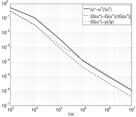
We now describe numerical experiments concerned with studying posterior consistency in the case . We let noting that if , then almost surely for all ; in particular . Thus as required. The forcing in is taken to be , where and with the canonical skew-symmetric matrix, and . The dimension of the attractor is determined by the viscosity parameter . For the particular forcing used there is an explicit steady state for all and for this solution is stable (see [26], Chapter 2 for details). As decreases the flow becomes increasingly complex and we focus subsequent studies of the inverse problem on the mildly chaotic regime which arises for . We use a time-step of . The data is generated by computing a true signal solving the Navier-Stokes equation at the desired value of , and then adding Gaussian random noise to it at each observation time. Furthermore, we let and take , so that . We take spatial observations at each observation time. The observations are made at the gridpoints; thus the observations include all numerically resolved, and hence observable, wavenumbers in the system. Since the noise is added in spectral space in practice, for convenience we define and present results in terms of . The same grid is used for computing the reference solution and for computing the MAP estimator.
Figure 1 illustrates the posterior consistency which arises as the observational noise strength . The three curves shown quantify: (i) the relative error of the MAP estimator compared with the truth, ; (ii) the relative error of compared with ; and (iii) the relative error of with respect to the observations . The figure clearly illustrates Theorem 16, via the dashed curve for (ii), and indeed shows that the map estimator itself is converging to the true initial condition, via the solid curve (i), as . Recall that the observations approach the true value of the initial condition, mapped forward under , as , and note that the dashed and dashed-dotted curves shows that the image of the MAP estimator under the forward operator , , is closer to than , asymptotically as .
6 Applications in Conditioned Diffusions
In this section we consider the MAP estimator for conditioned diffusions, including bridge diffusions and an application to filtering/smoothing. We identify the Onsager-Machlup functional governing the MAP estimator in three different cases. We demonstrate numerically that this functional may have more than one minimiser. Furthermore, we illustrate the results of the consistency theory in section 4 using numerical experiments. Subsection 6.1 concerns the unconditioned case, and includes the assumptions made throughout. Subsections 6.2 and 6.3 describe bridge diffusions and the filtering/smoothing problem respectively. Finally, subsection 6.4 is devoted to numerical experiments for an example in filtering/smoothing.
6.1 Unconditioned Case
For simplicity we restrict ourselves to scalar processes with additive noise, taking the form
| (32) |
If we let denote the measure on generated by the stochastic differential equation (SDE) given in (32), and the same measure obtained in the case , then the Girsanov theorem states that with density
If we choose an with , then an application of Itô’s formula gives
and using this expression to remove the stochastic integral we obtain
| (33) |
Thus, the measure has a density with respect to the Gaussian measure and (33) takes the form (1) with and : we have
where is defined by
| (34) |
and
We make the following assumption concerning the vector field driving the SDE:
Assumption 18.
The function in (32) satisfies the following conditions.
-
1.
for all .
-
2.
There is such that for all and for all .
Under these assumptions, we see that given by (34) satisfies Assumptions 1 and, indeed, the slightly stronger assumptions made in Theorem 7. Let denote the space of absolutely continuous functions on . Then the Cameron-Martin space for is
and the Cameron-Martin norm is given by
where
The mean of is the constant function and so, using Remark 2, we see that the Onsager-Machlup functional for the unconditioned diffusion (32) is thus given by
Together, Theorems 4 and 7 tell us that this functional attains its minimum over defined by
Furthermore such minimisers define MAP estimators for the unconditioned diffusion (32), i.e. the most likely paths of the diffusion.
We note that the regularity of minimisers for implies that the MAP estimator is , whilst sample paths of the SDE (32) are not even differentiable. This is because the MAP estimator defines the centre of a tube in which contains the most likely paths. The centre itself is a smoother function than the paths. This is a generic feature of MAP estimators for measures defined via density with respect to a Gaussian in infinite dimensions.
6.2 Bridge Diffusions
In this subsection we study the probability measure generated by solutions of (32), conditioned to hit at time so that , and denote this measure . Let denote the Brownian bridge measure obtained in the case . By applying the approach to determining bridge diffusion measures in [17] we obtain, from (33), the expression
| (35) |
Since is fixed we now define by
and then (35) takes again the form (1). The Cameron-Martin space for the (zero mean) Brownian bridge is
and the Cameron-Martin norm is again . The Onsager-Machlup function for the unconditioned diffusion (32) is thus given by
where , given by for all , is the mean of and
The MAP estimators for are found by minimising over .
6.3 Filtering and Smoothing
We now consider conditioning the measure on observations of the process at discrete time points. Assume that we observe given by
| (36) |
where and the are independent identically distributed random variables with . Let denote the -valued Gaussian measure and let denote the -valued Gaussian measure where is defined by
Recall and from the unconditioned case and define the measures and on as follows. The measure is defined to be an independent product of and , whilst . Then
with constant of proportionality depending only on . Clearly, by continuity,
and hence
Applying the conditioning Lemma 5.3 in [17] then gives
Thus we define
The Cameron-Martin space is again and the Onsager-Machlup functional is thus , given by
| (37) |
The MAP estimator for this setup is, again, found by minimising the Onsager-Machlup functional .
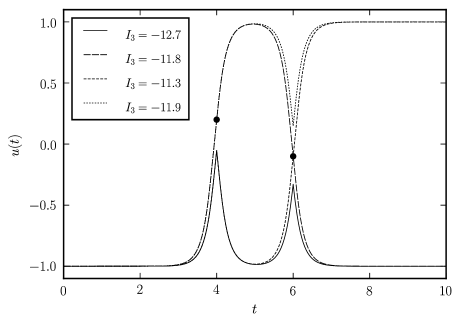
The only difference between the potentials and , and thus between the functionals for the unconditioned case and for the case with discrete observations, is the presence of the term . In the Euler-Lagrange equations describing the minima of , this term leads to Dirac distributions at the observation points and it transpires that, as a consequence, minimisers of have jumps in their first derivates at . This effect can be clearly seen in the local minima of shown in figure 2.
6.4 Numerical Experiments
In this section we perform three numerical experiments related to the MAP estimator for the filtering/smoothing problem presented in section 6.3.
For the experiments we generate a random “signal” by numerically solving the SDE (32), using the Euler-Maruyama method, for a double-well potential given by
with diffusion constant and initial value . From the resulting solution we generate random observations using (36). Then we implement the Onsager-Machlup functional from equation (37) and use numerical minimisation, employing the Broyden-Fletcher-Goldfarb-Shanno method (see [13]; we use the implementation found in the GNU scientific library [14]), to find the minima of . The same grid is used for numerically solving the SDE and for approximating the values of .
The first experiment concerns the problem of local minima of . For small number of observations we find multiple local minima; the minimisation procedure can converge to different local minima, depending on the starting point of the optimisation. This effect makes it difficult to find the MAP estimator, which is the global minimum of , numerically. The problem is illustrated in figure 2, which shows four different local minima for the case of observations. In the presence of local minima, some care is needed when numerically computing the MAP estimator. For example, one could start the minimisation procedure with a collection of different starting points, and take the best of the resulting local minima as the result. One would expect this problem to become less pronounced as the number of observations increases, since the observations will “pull” the MAP estimator towards the correct solution, thus reducing the number of local minima. This effect is confirmed by experiments: for larger numbers of observations our experiments found only one local minimum.
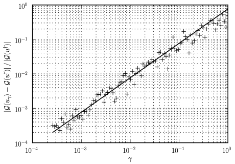
The second experiment concerns posterior consistency of the MAP estimator in the small noise limit. Here we use a fixed number of observations of a fixed path of (32), but let the variance of the observational noise converge to . Noting that the exact path of the SDE, denoted by in (27), has the regularity of a Brownian motion and therefore the observed path is not contained in the Cameron-Martin space , we are in the situation described in Corollary 17. Our experiments indicate that we have as , where denotes the MAP estimator corresponding to observational variance , confirming the result of Corollary 17. As discussed above, for small values of one would expect the minimum of to be unique and indeed experiments where different starting points of the optimisation procedure were tried did not find different minima for small . The result of a simulation with is shown in figure 3.
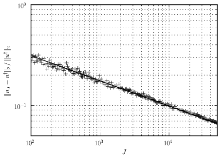
Finally, we perform an experiment to illustrate posterior consistency in the large sample size limit: for this experiment we still use one fixed path of the SDE (32). Then, for different values of , we generate observations using (36) at equidistantly spaced times , for fixed , and then determine the distance of the resulting MAP estimate to the exact path . As discussed above, for large values of one would expect the minimum of to be unique and indeed experiments where different starting points of the optimisation procedure were tried did not find different minima for large . The situation considered here is not covered by the theoretical results from section 4, but the results of the numerical experiment, shown in figure 4 indicate that posterior consistency still holds.
References
- [1] S. Agapiou, S. Larsson and A.M. Stuart. Posterior Consistency of the Bayesian Approach to Linear Ill-Posed Inverse Problems. arxiv.org/abs/1210.1563
- [2] A.F. Bennett. Inverse Modeling of the Ocean and Atmosphere. Cambridge University Press, 2002.
- [3] Bissantz N., Hohage T. and Munk A. 2004, Consistency and rates of convergence of nonlinear Tikhonov regularization with random noise. Inverse Problems 20, no. 6, 1773–1789.
- [4] Bochkina, N.A. Consistency of the posterior distribution in generalised linear inverse problems. arxiv.org/abs/1211.3382, 2012.
- [5] Bogachev, V. I. Gaussian measures. Mathematical Surveys and Monographs, 62. American Mathematical Society, Providence, RI, 1998.
- [6] Brown, L.D. and Low, M.G. Asymptotic equivalence of nonparametric regression and white noise. The Annals of Statistics 24(1996), 2384–2398.
- [7] S. L. Cotter, M. Dashti, J. C. Robinson, and A. M. Stuart. Bayesian inverse problems for functions and applications to fluid mechanics. Inverse Problems, 25(11):115008, 43, 2009.
- [8] SM Cox and PC Matthews. Exponential time differencing for stiff systems. Journal of Computational Physics, 176(2):430–455, 2002.
- [9] Dembo A. and Zeitouni O., Onsager-Machlup functionals and maximum a posteriori estimation for a class of non-Gaussian random fields. J. Mutivariate Analysis 36(1991), 243–262.
- [10] Da Prato G. & Zabczyk J. 1992, Stochastic equations in infinite dimensions. Encyclopedia of Mathematics and its Applications, 44. Cambridge University Press, Cambridge.
- [11] D. Dürr and A. Bach. The Onsager-Machlup function as lagrangian for the most probable path of a diffusion process. Communications in Mathematical Physics, 160:153–170, 1978.
- [12] Engl, H. W., Hanke, M. and Neubauer, A. 1996, Regularization of inverse problems. Mathematics and its Applications, 375. Kluwer Academic Publishers Group, Dordrecht.
- [13] R. Fletcher. Practical Methods of Optimization. Wiley-Blackwell, second edition, 2000.
- [14] M. Galassi, J. Davies, J. Theiler, B. Gough, G. Jungman, P. Alken, M. Booth, and F. Rossi. GNU Scientific Library Reference Manual. Network Theory Ltd., third edition, 2009.
- [15] Ghosal, S. and Ghosh, J.K. and Ramamoorthi, RV, Consistency issues in Bayesian nonparametrics. STATISTICS TEXTBOOKS AND MONOGRAPHS, 158(1999), 639–668.
- [16] Griebel, M. and Hegland, M. A Finite Element Method for Density Estimation with Gaussian Process Priors. SIAM Journal on Numerical Analysis, 47:4759–4792, 2010.
- [17] M. Hairer, A. M. Stuart, and J. Voss. Analysis of SPDEs arising in path sampling, part II: The nonlinear case. Annals of Applied Probability, 17:1657–1706, 2007.
- [18] M. Hairer, A. M. Stuart, and J. Voss. Signal processing problems on function space: Bayesian formulation, stochastic pdes and effective mcmc methods. The Oxford Handbook of Nonlinear Filtering, Editors D. Crisan and B. Rozovsky. Oxford University Press, 2011.
- [19] M. Hegland. Approximate maximum a posteriori with Gaussian process priors. Constructive Approximation, 26:205–224, 2007.
- [20] J.S. Hesthaven, S. Gottlieb, and D. Gottlieb. Spectral Methods for Time-Dependent Problems, volume 21. Cambridge Univ Pr, 2007.
- [21] Nobuyuki Ikeda and Shinzo Watanabe. Stochastic differential equations and diffusion processes. North-Holland Publishing Co., Amsterdam, second edition, 1989.
- [22] J. P. Kaipio and E. Somersalo. Statistical and Computational Inverse Problems. Springer, 2005.
- [23] Knapik, BT and van der Vaart, AW and van Zanten, JH, Bayesian inverse problems with Gaussian priors, Ann. Stat. 39(2011), 2626–2657.
- [24] M. Ledoux and M. Talagrand. Probability in Banach Spaces: Isoperimetry and Processes. Springer, 1991.
- [25] Lifshits M. A. 1995 Gaussian Random Functions, Kluwer Academic Pub.
- [26] A. Majda and X. Wang. Non-linear dynamics and statistical theories for basic geophysical flows. Cambridge Univ Pr, 2006.
- [27] Markussen, B. Laplace approximation of transition densities posed as Brownian expectations. Stochastic Processes and their Applications 119(2009), p 208–231.
- [28] Mortensen, R.E. Maximum-likelihood recursive filtering. Journal of Optimization Theory and Applications 2(1968), 386–393.
- [29] K. Ray. Bayesian inverse problems with non-conjugate priors. arXiv:1209.6156, 2012.
- [30] C. E. Rasmussen and C. K. I. Williams. Gaussian Processes for Machine Learning. The MIT Press, 2006.
- [31] J. C. Robinson, Infinite-Dimensional Dynamical Systems, Cambridge Texts in Applied Mathematics, Cambridge University Press, Cambridge, 2001.
- [32] Rogers, C. Least-action filtering. http://www.statslab.cam.ac.uk/ chris/papers/LAF.pdf
- [33] Stuart A. M. 2010, Inverse Problems: A Bayesian Approach. Acta Numerica 19.
- [34] Zeitouni O. 1989, On the Onsager-Machlup Functional of Diffusion Processes Around Non C2 Curves. Annals of Probability 17(1989), pp. 1037–1054.
- [35] Zeitouni O. 2000, MAP estimators of diffusions: an updated account. Systems Theory: Modeling, Analysis and Control, 518(2000), page 145.