Multi-Layer Hybrid-ARQ
for an Out-of-Band Relay Channel

Abstract

This paper addresses robust communication on a fading relay channel in which the relay is connected to the decoder via an out-of-band digital link of limited capacity. Both the source-to-relay and the source-to-destination links are subject to fading gains, which are generally unknown to the encoder prior to transmission. To overcome this impairment, a hybrid automatic retransmission request (HARQ) protocol is combined with multi-layer broadcast transmission, thus allowing for variable-rate decoding. Moreover, motivated by cloud radio access network applications, the relay operation is limited to compress-and-forward. The aim is maximizing the throughput performance as measured by the average number of successfully received bits per channel use, under either long-term static channel (LTSC) or short-term static channel (STSC) models. In order to opportunistically leverage better channel states based on the HARQ feedback from the decoder, an adaptive compression strategy at the relay is also proposed. Numerical results confirm the effectiveness of the proposed strategies.

I Introduction

Consider the fading relay channel model shown in Fig. 1, in which an encoder communicates to a decoder through a relay that is connected to the decoder via an out-of-band capacity-constrained backhaul link. Both the source-to-relay and the source-to-destination links are subject to fading. The motivation for this model comes from the uplink of cloud radio access networks [1][2], in which base stations (BSs) operate as soft relays that communicate with a central decoder via a digital backhaul links. In this scenario, the central decoder performs decoding based on the compressed signals collected from the connected BSs. With regards to this application, in the model of Fig. 1, the encoder represents a mobile station (MS); the relay is the BS in the same cell, which is connected to the (central) decoder via backhaul link; and the signal $Y$ represents the compressed signals collected by the decoder from BSs belonging to other cells. The signal $Y$ can be seen as side information available at the decoder when designing the encoder (i.e., the MS) and relay (i.e., the BS).

The fading relay channel was investigated in [3] and [4] in the absence of the direct link between the source and the destination and assuming fading also on the relay-to-destination link. In [3], various relaying protocols including decode-and-forward, quantize-and-forward and hybrid amplify-quantize-and-forward were developed in combination with layered broadcast coding (BC). This work was extended in [4] by studying infinite-layer coding at both the source and the relay in conjunction with decode-and-forward relaying.

The fading relay channels with a direct link between the source and the destination (as in Fig. 1) was studied in [5]-[12]. The works in [5]-[7] solved the problem of optimizing the compression strategy at the relay under the assumption of perfect channel state information for multi-antenna terminals. In the presence of uncertainty on the fading coefficient $S$, layered approaches that adopt a competitive, rather than average, optimality criterion are derived in [11] and [12] assuming no hybrid automatic retransmission request (HARQ). In all the previous works, the feedback link in Fig. 1 was not included. This link is used in this paper to enable HARQ.

I-A Contributions

In this work, motivated by cloud radio access applications as mentioned above, we study the system in Fig. 1, assuming that the relay performs compress-and-forward. We propose to combine two key strategies to mitigate the impact of the fading on the source-to-relay and source-to-destination links, namely, HARQ and BC. With HARQ, the decoder requests retransmission by sending feedback information to the encoder and the relay regarding the outcome of the decoding process. Specifically, the incremental redundancy HARQ (IR-HARQ) consists of the transmission of additional parity bits in case of failed decoding [13]. With BC [14]-[16], instead, one allows for variable-rate decoding that opportunistically adapts to the actual fading state conditions.

Multi-layer HARQ strategies have thus the advantage of allowing for variable-length transmission and variable-rate decoding, and were introduced in [17] for point-to-point fading channels. As in [17], we aim at maximizing the average throughput and distinguish two scenarios, namely short-term static channel (STSC) and long-term static channel (LTSC). Moreover, for the LTSC scenario, we propose an adaptive compression method at the relay that is able to opportunistically leverage better fading state based on the feedback information received from the decoder. The effectiveness of the proposed multi-layer HARQ strategies is confirmed via extensive numerical results.

The paper is organized as follows. We state the system model in Sec. II and establish the problem formulation in Sec. III. After describing the proposed multi-layer HARQ strategies with a constant compression gain and adaptive compression gain in Sec. IV and Sec. V, respectively, for the LTSC model, we extend the discussion to the STSC model in Sec. VI. Numerical results are provided in Sec. VII to demonstrate the performance gain of the proposed multi-layer HARQ strategies.

Notation: We adopt standard information-theoretic definitions for the mutual information $I(X;Y)$ between the random variables $X$ and $Y$, and conditional mutual information $I(X;Y|Z)$ between $X$ and $Y$ conditioned on random variable $Z$ [18]. All logarithms are in base two unless specified. We use $\mathbb{E}_{X}[\cdot]$ to denote the expectation over $X$. For a real number $x$, we define a function $[x]^{+}=\max\{x,0\}$.

II System Model

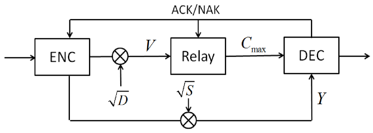
Figure 1: A fading relay channel with out-of-band relay-to-decoder communication and a feedback link to enable HARQ.

We consider the fading relay channel depicted in Fig. 1, in which the relay is connected to the decoder via a digital link of capacity $C_{\max}$. In order to enable HARQ, after each transmission block (or slot), the decoder sends feedback information to the encoder acknowledging, or not, successful decoding. This feedback link is assumed to be error-free.

II-A Channel Model

The signal $V_{t,i}$ received by the relay in the $i$th symbol, $i=1,\ldots,n$, of the $t$th transmission slot is given as

$$V_{t,i}=\sqrt{D_{t}}X_{t,i}+E_{t,i},$$ (1)

for $t=1,\ldots,T$, where $D_{t}$ is the fading coefficient in the $t$th time slot, $X_{t,i}\sim\mathcal{N}(0,P)$ represents the signal transmitted by the encoder, $E_{t,i}\sim\mathcal{N}(0,1)$ is the additive noise at the relay, and $T$ is the maximum tolerable delay for the HARQ process. As it will be detailed, upon correct decoding at the destination, the HARQ process is stopped, and $T$ is the maximum number of overall transmissions allowed for the same data packet. We assume that the block size $n$ is large enough to enable the use of information-theoretic limits. The notation $D_{t}$ has been chosen with reference to the cloud radio access application in which $D_{t}$ represents the direct channel to the local BS.

The symbol $Y_{t,i}$ received by the decoder in the $i$th symbol, $i=1,\ldots,n$, of the $t$th transmission slot is

$$Y_{t,i}=\sqrt{S_{t}}X_{t,i}+Z_{t,i},$$ (2)

for $t=1,\ldots,T$, where $S_{t}$ is the fading coefficient in the $t$th time slot, and $Z_{t,i}\sim\mathcal{N}(0,1)$ is the additive noise. The notation $S_{t}$ is a reminder that in the cloud radio access application, $S_{t}$ represents the side information channel (see Sec. I). From now on, we omit the symbol index $i$ for notational brevity.

Following [17], depending on the channel coherence time, we distinguish two scenarios: i) short-term static channel (STSC); and ii) long-term static channel (LTSC). With LTSC, the channels remain fixed over all the, at most, $T$ transmission blocks used for the current data packet, that is,

$$D_{t}=D\,\,\mathrm{and}\,\,S_{t}=S,\,\,\mathrm{for\,\,all}\,\,t=1,\ldots,T.$$ (3)

In contrast, with STSC, the channel changes independently from block to block. We first study the LTSC model (3) in Sec. IV and Sec. V, and then consider the STSC case in Sec. VI. We assume that the fading coefficients $D_{t}$ in (1) and $S_{t}$ in (2) are independent, and have arbitrary CDFs $F_{D}(d)=\Pr[D_{t}\leq d]$ and $F_{S}(s)=\Pr[S_{t}\leq s]$ with finite powers $\rho_{D}=\mathbb{E}[|D|^{2}]$ and $\rho_{S}=\mathbb{E}[|S|^{2}]$, respectively.

The realization of the fading coefficients $S_{t}$ is known only to the decoder, while that of the fading coefficients $D_{t}$ is available at the decoder as well as the relay. In order to study the effect of the local CSI at the encoder, we will consider both cases where the encoder knows the realization of the “direct” fading channel $D_{t}$ to the relay, e.g., through feedback, or not.

II-B Relay Operation

The relay compresses its received signal $V_{t}$ and sends a description $W_{t}$ to the decoder. Without claim of optimality, we assume a Gaussian test channel (see, e.g., [18]) as

$$W_{t}=\sqrt{a_{t}}V_{t}+N_{t},$$ (4)

where $a_{t}$ is a non-negative compression gain and $N_{t}\sim\mathcal{N}(0,1)$ represents the compression noise. Using binning for distributed source coding at the relay by leveraging the side information (2) at the decoder, the latter can recover the description $W_{t}$ as long as the inequality

$$I(V_{t};W_{t}|Y_{t})=\frac{1}{2}\log\left(1+a_{t}\left(\frac{1}{D_{t}}+\frac{P}{1+PS_{t}}\right)\right)\leq C_{\max}$$ (5)

is satisfied [18, Ch. 11]. Due to the mentioned CSI limitation, the relay should compute the compression gain $a_{t}$ as a function of the realization of the local fading $D_{t}$ without having information about the fading state $S_{t}$ in (2). Therefore, in order to guarantee that the decoder can always recover $W_{t}$ regardless of the realization of the fading coefficient $S_{t}$ on the side information (2), one needs to set the compression gain $a_{t}$ so that (5) is satisfied even for the minimum value $s_{\min}$ in the support of $F_{S}(s)$ (i.e., $s_{\min}=\mathrm{inf}\{s:F_{S}(s)>0\}$). This leads to

$$a_{t}=\frac{\beta(1+s_{\min}P)}{1/d+(1+s_{\min}/d)P}\triangleq a_{d},$$ (6)

where $\beta=2^{2C_{\max}}-1$, for $D_{t}=d$. We will consider different strategies for the choice of the compression gain $a_{t}$ in Sec. IV and Sec. V.

II-C Multi-Layer Hybrid-ARQ

Following [17], the encoder uses a two-layer BC transmission strategy coupled with HARQ, which is described next. The encoder wishes to deliver two messages $M_{1}\in\{1,\ldots,2^{nR_{1}}\}$ and $M_{2}\in\{1,\ldots,2^{nR_{2}}\}$, which are independent and uniformly distributed, to the decoder. To this end, it maps message $M_{l}$ to a $n$-symbol codeword $X_{l,t}^{n}$ for $l=1,2$. We assume independent Gaussian codebooks across the $T$ blocks, that is, the codewords $X_{l,t}^{n}$ are independently generated with i.i.d. symbols $\mathcal{N}(0,1)$ for all blocks $t=1,\ldots,T$. To describe the multi-layer HARQ strategy, we distinguish the following two transmission modes: i) BC mode; and ii) single-layer (SL) mode. In the BC mode, the encoder transmits the superposition

$$X_{t}=\sqrt{\alpha P}X_{1,t}+\sqrt{\bar{\alpha}P}X_{2,t},$$ (7)

for each symbol, where $\alpha\in[0,1]$ and $\bar{\alpha}=1-\alpha$ represent the fractions of powers allocated to the first and second layers, respectively. In contrast, in the SL mode, the encoder transmits only the second-layer codeword with full power $P$, and the transmitted signal $X_{t}$ is written as

$$X_{t}=\sqrt{P}X_{2,t}.$$ (8)

In the first slot $t=1$, the encoder emits the signal $X_{1}$ in the BC mode (7) and the relay sends the compressed version $W_{1}$ in (4) of the received signal $V_{1}$ to the decoder. At the completion of the slot, the decoder first tries to decode the message $M_{1}$; if successful, it cancels the codeword $X_{1,1}$ from the received signal and attempts to decode message $M_{2}$. Decoding is based on the received signal in slot $t$, which can be written as

$$\bar{Y}_{t}=\left[\begin{array}[]{c}W_{t}\\ Y_{t}\end{array}\right]=\left[\begin{array}[]{c}\sqrt{a_{t}D_{t}}\\ \sqrt{S_{t}}\end{array}\right]X_{t}+\left[\begin{array}[]{c}\sqrt{a_{t}D_{t}}E_{t}+N_{t}\\ Z_{t}\end{array}\right],$$ (9)

for $t=1,\ldots,T$.

The decoder informs the encoder and the relay about the number of layers that were correctly decoded. If both messages are not correctly decoded, in the next slot $t=2$, the encoder sends incremental redundancy information for both layers using the BC mode (7). Note that incremental redundancy entails that, as mentioned, the codebooks used at different blocks are independent (see, e.g., [13]). Instead, if only the first layer $M_{1}$ was decoded in the first slot, the encoder transmits incremental redundancy information only for the second layer by using the SL mode (8). This process lasts until either both messages $M_{1}$ and $M_{2}$ are decoded successfully or the maximum number $T$ of transmissions is reached. Therefore, if a message $M_{l}$ is not decoded until the $T$th slot, outage is declared for layer $l$.

III Problem Definition

The problem of interest is the maximization of the expected throughput $\eta$ as measured by the average number of successfully received bits per channel use. Using the renewal theorem (see, e.g., [19]), we can calculate the expected throughput $\eta$ as

$$\eta=\frac{\mathbb{E}\left[\mathtt{R}\right]}{\mathbb{E}\left[\mathtt{L}\right]},$$ (10)

where $\mathbb{E}\left[\mathtt{R}\right]$ is the average rate decoded in a HARQ session, which consists of at most $T$ transmissions, and $\mathbb{E}\left[\mathtt{L}\right]$ is the expected number of transmission blocks for HARQ session. Expectations are taken with respect to the fading coefficients $D_{t}$ and $S_{t}$. These quantities can be computed as [17]

$$\mathbb{E}\left[\mathtt{R}\right] =R_{1}\left(1-p_{\mathrm{out}}^{1}(T)\right)+R_{2}\left(1-p_{\mathrm{out}}^{2}(T)\right),$$ (11)

$$\mathrm{and}\,\,\mathbb{E}\left[\mathtt{L}\right] =\sum_{t=1}^{T-1}tp_{\mathrm{dec}}^{2}(t)+T\left(p_{\mathrm{dec}}^{2}(T)+p_{\mathrm{out}}^{2}(T)\right),$$ (12)

where the probabilities $p_{\mathrm{out}}^{l}(k)$ and $p_{\mathrm{dec}}^{l}(k)$ are defined as

$$p_{\mathrm{out}}^{l}(k) =\Pr\left[M_{l}\,\mathrm{is\,not\,decoded\,until\,slot}\,k\right],$$ (13)

$$\mathrm{and}\,\,p_{\mathrm{dec}}^{l}(k) =\Pr\left[M_{l}\,\mathrm{is\,decoded\,in\,slot}\,k\right].$$ (14)

The probabilities $p_{\mathrm{out}}^{l}(k)$ and $p_{\mathrm{dec}}^{l}(k)$ depend on the parameters $R_{1}$, $R_{2}$ and $\alpha$ as will be clarified in the next sections. The problem of maximizing the average throughput $\eta$ is then formulated as

$$\underset{R_{1},R_{2}\geq 0,\,\alpha\in[0,1]}{\mathrm{maximize}}\,\,\eta(R_{1},R_{2},\alpha),$$ (15)

where we have made explicit the dependence on $(R_{1},R_{2},\alpha)$. As a benchmark, it is useful to consider the single-layer scheme obtained as a special case of the proposed strategy with $R_{2}=0$ and $\alpha=1$. Thus, the optimal throughput of a single-layer strategy is the solution of the following problem:

$$\underset{R_{1}\geq 0}{\mathrm{maximize}}\,\,\eta(R_{1},0,1).$$ (16)

IV Constant Compression Gain

In this section, we analyze the throughput of the proposed multi-layer HARQ strategy when the relay uses a constant compression gain $a_{t}=a_{D_{t}}$ as in (6) for all $t=1,\ldots,T$ regardless of the feedback information reported from the decoder. As explained in Sec. II, with this choice, the description $W_{t}$ can be recovered at the decoder for all realizations of the fading channel $S_{t}$. However, this approach is not able to opportunistically leverage a more advantageous fading state $S_{t}$. A strategy that can exploit better fading state via adaptive compression will be discussed in Sec. V. We focus on the LTSC model, so that $D_{t}=D$ and $S_{t}=S$ for all $t=1,\ldots,T$. Moreover, we study both the case with local CSI at the encoder, i.e., when the encoder knows the local fading state $D=d$ and thus can choose the tuple $(R_{1}(d),R_{2}(d),\alpha(d))$ as a function of $d$, and the case with no local CSI at the encoder.

To express the objective throughput $\eta$ in (10), we have to compute the probabilities in (13) and (14) as a function of parameters $R_{1}$, $R_{2}$ and $\alpha$ which is done in the following lemmas.

Lemma 1.

The probability $p_{\mathrm{out}}^{1}(k)$ with compression gain $a_{D}$ is given as

$$p_{\mathrm{out}}^{1}(k) =\mathbb{E}_{D}\left[\theta(D)\right]$$ (17)

where the function $\theta(d)$ is defined as

$$\theta(d)=\begin{cases}F_{S}\left(\frac{\zeta_{1}(d,1)}{\bar{\zeta}_{1}(d,1)P}+\frac{a_{d}}{b_{d}}\right),&\mathrm{if}\,\,\bar{\zeta}_{1}(d,1)\leq 0\\ 1,&\mathrm{if}\,\,\bar{\zeta}_{1}(d,1)>0\end{cases},$$

with $b_{d}\triangleq 1+a_{d}/d$ and the functions $\zeta_{i}(d,l)$ and $\bar{\zeta}_{i}(d,l)$ given as

$$\zeta_{i}(d,l)= 2^{2R_{i}(d)/l}-1,$$ (18)

$$\mathrm{and}\,\,\bar{\zeta}_{i}(d,l)= 2^{2R_{i}(d)/l}\bar{\alpha}(d)-1,$$ (19)

for $i=1,2$ and $k=1,\ldots,T$.

Proof.

The proof is in Appendix A-A.

∎

Lemma 2.

If $\bar{\alpha}P\ll 1$, the probability $p_{\mathrm{out}}^{2}(k)$ with compression gain $a_{D}$ is approximated as

$$p_{\mathrm{out}}^{2}(k)\approx p_{\mathrm{out}}^{1}(k)+\sum_{l=1}^{k}\mathbb{E}_{D}\left[\left[F_{S}(v_{k,l}^{\mathrm{UB}}(D))-F_{S}(v_{l}^{\mathrm{LB}}(D))\right]^{+}\right],$$ (20)

where $v_{l}^{\mathrm{LB}}(d)$ and $v_{k,l}^{\mathrm{UB}}(d)$ are defined as

$$v_{l}^{\mathrm{LB}}(d)= \begin{cases}-\left[-\frac{\zeta_{1}(d,l)}{\bar{\zeta}_{1}(d,l)P}-\frac{a_{d}}{b_{d}}\right]^{+},&\mathrm{if}\,\bar{\zeta}_{1}(d,l)<0\\ \infty,&\mathrm{if}\,\bar{\zeta}_{1}(d,l)\geq 0\end{cases},$$ (21)

$$\mathrm{and}\,\,v_{k,l}^{\mathrm{UB}}(d)= \min\mathcal{V}_{k,l}^{\mathrm{UB}},$$ (22)

with the set $\mathcal{V}_{k,l}^{\mathrm{UB}}$ given as

$$\mathcal{V}_{k,l}^{\mathrm{UB}}=\left\{\hat{v}_{k,l}^{\mathrm{UB}}(d)\right\}\cup\begin{cases}\textrm{\O},&\mathrm{if}\,\bar{\zeta}_{1}(d,l-1)\geq 0\\ \left\{\left[-\frac{\zeta_{1}(d,l-1)}{\bar{\zeta}_{1}(d,l-1)P}-\frac{a_{d}}{b_{d}}\right]^{+}\right\},&\mathrm{if}\,\bar{\zeta}_{1}(d,l-1)<0\end{cases}.$$ (23)

We have defined the function $\hat{v}_{k,l}^{\mathrm{UB}}(d)$ as

$$\hat{v}_{k,l}^{\mathrm{UB}}(d)=\begin{cases}\infty,&\mathrm{if}\,\,k=l\,\mathrm{and}\,\frac{2^{2R_{2}(d)}b_{d}^{k}}{c(d)^{l}}>1\\ 0,&\mathrm{if}\,\,k=l\,\mathrm{and}\,\frac{2^{2R_{2}(d)}b_{d}^{k}}{c(d)^{l}}\leq 1\\ \left[\frac{\left(\zeta_{2}(d,k-l)+1\right)b_{d}^{k/(k-l)-1}}{Pc(d)^{l/(k-l)}}-\frac{a_{d}}{b_{d}}-\frac{1}{P}\right]^{+},&\mathrm{if}\,\,k>l\end{cases},$$ (24)

with the function $c(d)$ given as $c(d)=b_{d}+\bar{\alpha}(d)Pa_{d}$.

Proof.

See Appendix A-B.

∎

Lemma 3.

If $\bar{\alpha}P\ll 1$, the probability $p_{\mathrm{dec}}^{2}(k)$ with compression gain $a_{D}$ is approximated as

$$p_{\mathrm{dec}}^{2}(k)\approx \sum_{l=1}^{k-1}\mathbb{E}_{D}\left[\left[F_{S}(u_{k,l}^{\mathrm{UB}}(D))-F_{S}(u_{k,l}^{\mathrm{LB}}(D))\right]^{+}\right]+\mathbb{E}_{D}\left[\left[F_{S}(q_{k}^{\mathrm{UB}}(D))-F_{S}(q_{k}^{\mathrm{LB}}(D))\right]^{+}\right],$$ (25)

where $u_{k,l}^{\mathrm{LB}}(d)$, $u_{k,l}^{\mathrm{UB}}(d)$, $q_{k}^{\mathrm{LB}}(d)$ and $q_{k}^{\mathrm{UB}}(d)$ are defined as

$$u_{k,l}^{\mathrm{LB}}(d)= \max\mathcal{U}_{k,l}^{\mathrm{LB}},$$

$$u_{k,l}^{\mathrm{UB}}(d)= \min\mathcal{U}_{k,l}^{\mathrm{UB}},$$

$$q_{k}^{\mathrm{LB}}(d)= \max\mathcal{Q}_{k}^{\mathrm{LB}},$$

$$\mathrm{and}\,\,q_{k}^{\mathrm{UB}}(d)= \begin{cases}-\frac{\zeta_{1}(d,k-1)}{\bar{\zeta}_{1}(d,k-1)P}-\frac{a_{d}}{b_{d}},&\mathrm{if}\,\bar{\zeta}_{1}(d,k-1)<0\\ \infty,&\mathrm{if}\,\bar{\zeta}_{1}(d,k-1)\geq 0\end{cases},$$

with the sets $\mathcal{U}_{k,l}^{\mathrm{LB}}$, $\mathcal{U}_{k,l}^{\mathrm{UB}}$ and $\mathcal{Q}_{k}^{\mathrm{LB}}$ given as

$$\mathcal{U}_{k,l}^{\mathrm{LB}}= \left\{\hat{u}_{k,l}^{\mathrm{LB}}(d)\right\}\cup\begin{cases}\left\{-\frac{\zeta_{1}(d,l)}{\bar{\zeta}_{1}(d,l)P}-\frac{a_{d}}{b_{d}}\right\},&\mathrm{if}\,\bar{\zeta}_{1}(d,l)<0\\ \{\infty\},&\mathrm{if}\,\bar{\zeta}_{1}(d,l)\geq 0\end{cases},$$ (26)

$$\mathcal{U}_{k,l}^{\mathrm{UB}}= \left\{\hat{u}_{k,l}^{\mathrm{UB}}(d)\right\}\cup\begin{cases}\left\{-\frac{\zeta_{1}(d,l-1)}{\bar{\zeta}_{1}(d,l-1)P}-\frac{a_{d}}{b_{d}}\right\},&\mathrm{if}\,\bar{\zeta}_{1}(d,l-1)<0\\ \textrm{\O},&\mathrm{if}\,\bar{\zeta}_{1}(d,l-1)\geq 0\end{cases},$$ (27)

$$\mathrm{and}\,\,\mathcal{Q}_{k}^{\mathrm{LB}}= \left\{\left[\frac{\zeta_{2}(d,k)}{\bar{\alpha}(d)P}-\frac{a_{d}}{b_{d}}\right]^{+}\right\}\cup\begin{cases}\left\{-\frac{\zeta_{1}(d,k)}{\bar{\zeta}_{1}(d,k)P}-\frac{a_{d}}{b_{d}}\right\},&\mathrm{if}\,\bar{\zeta}_{1}(d,k)<0\\ \{\infty\},&\mathrm{if}\,\bar{\zeta}_{1}(d,k)\geq 0\end{cases}.$$

We have defined the functions $\hat{u}_{k,l}^{\mathrm{LB}}(d)$ and $\hat{u}_{k,l}^{\mathrm{UB}}(d)$ as

$$\hat{u}_{k,l}^{\mathrm{LB}}(d)= \left[\frac{\left(\zeta_{2}(d,k-1)+1\right)b_{d}^{k/(k-1)-1}}{Pc(d)^{l/(k-l)}}-\frac{a_{d}}{b_{d}}-\frac{1}{P}\right]^{+},$$ (28)

$$\hat{u}_{k,l}^{\mathrm{UB}}(d)= \begin{cases}\infty,&\mathrm{if}\,l=k-1\,\mathrm{and}\,\frac{2^{2R_{2}(d)}b_{d}^{k-1}}{c(d)^{l}}>1\\ 0&\mathrm{if}\,l=k-1\,\mathrm{and}\,\frac{2^{2R_{2}(d)}b_{d}^{k-1}}{c(d)^{l}}\leq 1\\ \left[\frac{\left(\zeta_{2}(d,k-1-l)+1\right)b_{d}^{(k-1)/(k-1-l)-1}}{Pc(d)^{l/(k-1-l)}}-\frac{a_{d}}{b_{d}}-\frac{1}{P}\right]^{+},&\mathrm{if}\,l<k-1\end{cases}.$$ (29)

Proof.

The proof appears in Appendix A-C.

∎

With Lemmas 1-3, we can express the throughput (10) as a function of the optimization variables $R_{1}$, $R_{2}$ and $\alpha$ via numerical integration over the distribution $F_{D}(d)$. The optimization problems (15) and (16) are not convex and need to be solved via global optimization tool such as the branch-and-bound method [20]. Specifically, with local CSI at the encoder, one needs to optimize over the parameters $R_{1}(d)$, $R_{2}(d)$ and $\alpha(d)$, which corresponds to the tuple $(R_{1},R_{2},\alpha)$ to be used when the relay fading state is $D_{t}=d$. In practice, this optimization can be reformulated by quantizing the fading distribution. Instead, without local CSI at the encoder, the optimization is done over the single tuple $(R_{1},R_{2},\alpha)$ since the encoder is not able to adapt to the fading state $D$.

V Adaptive Compression Gain

In the previous section, we have assumed that the relay employs Gaussian test channel (4) with compression gain $a_{t}=a_{D}$ for all $t=1,\ldots,T$ regardless of the feedback information reported from the decoder under the LTSC (3). We recall that this choice guarantees reliable decompression even in the worst-case fading state $S_{t}=s_{\min}$. This section is motivated by the attempt to leverage better fading states when they occur. To this end, we assume that the feedback information that only the message $M_{1}$ of the first layer was decoded in a slot $k$ implies that the fading coefficient $S_{t}$ of the side information $Y_{t}$ is larger than some level $\hat{s}$, that is, $S\geq\hat{s}$. This can be calculated as

$$\hat{s}=\max\left\{\frac{\left[(2^{2R_{1}/k}-1)b_{D}+(2^{2R_{1}/k}\bar{\alpha}-1)Pa_{D}\right]^{+}}{b_{D}(1-2^{2R_{1}/k}\bar{\alpha})P},\,s_{\min}\right\}$$ (30)

by imposing the condition that the accumulated mutual information is sufficient to support rate $R_{1}$ (see Appendix A for more discussion). Upon reception of a positive acknowledgement for layer 1 and a negative acknowledgement for layer 2, we then propose that, from the next slot $t>k$, the relay performs compression assuming the better side information $S_{t}=\hat{s}\geq s_{\min}$. The corresponding compression gain is given as

$$a_{t}=\frac{\beta(1+\hat{s}P)}{1/D+(1+\hat{s}/D)P}\triangleq\hat{a}_{D}.$$ (31)

With adaptive compression, the expected throughput $\eta$ in (10) can be computed using the lemmas presented in the previous section with the changes discussed in the following lemmas.

Lemma 4.

If $\bar{\alpha}P\ll 1$, the probability $p_{\mathrm{out}}^{2}(k)$ with adaptive compression is approximated as (20) in Lemma 2 with $\hat{v}_{k,l}^{\mathrm{UB}}(d)$ modified as

$$\hat{v}_{k,l}^{\mathrm{UB}}(d)=\begin{cases}\infty,&\mathrm{if}\,\,k=l\,\mathrm{and}\,\frac{2^{2R_{2}(d)}b_{d}^{l}}{c(d)^{l}}>1\\ 0,&\mathrm{if}\,\,k=l\,\mathrm{and}\,\frac{2^{2R_{2}(d)}b_{d}^{l}}{c(d)^{l}}\leq 1\\ \left[\frac{\left(\zeta_{2}(d,k-l)+1\right)b_{d}^{l/(k-l)}}{Pc(d)^{l/(k-l)}}-\frac{\hat{a}_{d}}{\hat{b}_{d}}-\frac{1}{P}\right]^{+},&\mathrm{if}\,\,k>l\end{cases},$$ (32)

where $\hat{b}_{d}\triangleq 1+\hat{a}_{d}/d$.

Proof.

See Appendix B-A.

∎

Lemma 5.

If $\bar{\alpha}P\ll 1$, the probability $p_{\mathrm{dec}}^{2}(k)$ with adaptive compression is approximated as (25) in Lemma 3 with $\hat{u}_{k,l}^{\mathrm{LB}}(d)$ and $\hat{u}_{k,l}^{\mathrm{UB}}(d)$ modified as

$$\hat{u}_{k,l}^{\mathrm{LB}}(d)= \left[\frac{\left(\zeta_{2}(d,k-l)+1\right)b_{d}^{l/(k-l)}}{Pc(d)^{l/(k-l)}}-\frac{\hat{a}_{d}}{\hat{b}_{d}}-\frac{1}{P}\right]^{+},$$ (33)

$$\hat{u}_{k,l}^{\mathrm{UB}}(d)= \begin{cases}\infty,&\mathrm{if}\,\,l=k-1\,\mathrm{and}\,\frac{2^{2R_{2}(d)}b_{d}^{l}}{c(d)^{l}}>1\\ 0,&\mathrm{if}\,\,l=k-1\,\mathrm{and}\,\frac{2^{2R_{2}(d)}b_{d}^{l}}{c(d)^{l}}\leq 1\\ \left[\frac{\left(\zeta_{2}(d,k-1-l)+1\right)b_{d}^{l/(k-1-l)}}{Pc(d)^{l/(k-1-l)}}-\frac{\hat{a}_{d}}{\hat{b}_{d}}-\frac{1}{P}\right]^{+},&\mathrm{if}\,\,l<k-1\end{cases}.$$ (34)

Proof.

See Appendix B-B.

∎

With the results in Lemmas 1, 4 and 5, we can express the average throughput with the adaptive compression described in this section as a function of the design parameters $R_{1}$, $R_{2}$ and $\alpha$.

VI Short-Term Static Channels

In this section, we discuss the STSC model in which the channel coefficients $D_{t}$ and $S_{t}$ change independently from block to block. For simplicity, as in [17], we focus on the case $T=2$, i.e., there can be at most one retransmission. It is observed that, even with $T=2$, we have to consider four random variables $D_{1}$, $D_{2}$, $S_{1}$ and $S_{2}$, which complicate the analysis as compared to the LTSC model. Moreover, given the independence of the channel fading gains from block to block, adaptive compression is not applicable under the STSC model. Therefore, we set the compression gains as $a_{t}=a_{D_{t}}$ in (6) for $t=1,2$. The quantities in (11) and (12) reduce to

$$\mathbb{E}\left[\mathtt{R}\right] =R_{1}\left(1-p_{\mathrm{out}}^{1}(2)\right)+R_{2}\left(1-p_{\mathrm{out}}^{2}(2)\right),$$ (35)

$$\mathrm{and}\,\,\mathbb{E}\left[\mathtt{L}\right] =p_{\mathrm{dec}}^{2}(1)+2\left(1-p_{\mathrm{dec}}^{2}(1)\right).$$ (36)

Thus, it is enough to compute three probabilities $p_{\mathrm{out}}^{1}(2)$, $p_{\mathrm{out}}^{2}(2)$ and $p_{\mathrm{dec}}^{2}(1)$, which are derived in the following lemmas.

Lemma 6.

The probability $p_{\mathrm{out}}^{1}(2)$ in the STSC model with $T=2$ is given as

$$p_{\mathrm{out}}^{1}(2)=\mathbb{E}_{D_{1},D_{2},S_{1}}\left[g(D_{1},D_{2},S_{1})\right],$$ (37)

where we have defined the function $g(d_{1},d_{2},s_{1})$ as

$$g(d_{1},d_{2},s_{1}) =\begin{cases}F_{S_{2}}\left(\frac{\left[(2^{2h(d_{1},s_{1})}-1)b_{d_{2}}+(2^{2h(d_{1},s_{1})}\bar{\alpha}-1)a_{d_{2}}P\right]^{+}}{(2^{2h(d_{1},s_{1})}\bar{\alpha}-1)b_{d_{2}}P}\right),&\mathrm{if}\,\,2^{2h(d_{1},s_{1})}\bar{\alpha}<1\\ 0,&\mathrm{if}\,\,h(d_{1},s_{1})=0\,\mathrm{and}\,\bar{\alpha}=1\\ 1,&\mathrm{otherwise}\end{cases},$$ (38)

with the function $h(d_{1},s_{1})$ given as

$$h(d_{1},s_{1})= R_{1}-f_{\mathrm{I}}\left(\alpha P,\bar{\alpha}P,a_{d_{1}},s_{1},d_{1}\right).$$ (39)

The function $f_{\mathrm{I}}(P,\bar{P},a,s,d)$ is defined as

$$f_{\mathrm{I}}(P,\bar{P},a,s,d)=\frac{1}{2}\log\left(1+P\frac{s+a(1+s/d)}{1+a/d+\bar{P}\left(s+a(1+s/d)\right)}\right).$$ (40)

Proof.

See Appendix C.

∎

Lemma 7.

The probability $p_{\mathrm{out}}^{2}(2)$ in the STSC model with $T=2$ is given as

$$p_{\mathrm{out}}^{2}(2)= \mathbb{E}_{D_{1},D_{2},S_{1}}\left[\varphi(D_{1},D_{2},S_{1})\right]+\mathbb{E}_{D_{1},D_{2},S_{1}}\left[\gamma(D_{1},D_{2},S_{1})\right]+p_{\mathrm{out}}^{1}(2),$$ (41)

where the functions $\varphi(d_{1},d_{2},s_{1})$ and $\gamma(d_{1},d_{2},s_{1})$ are defined as

$$\varphi(d_{1},d_{2},s_{1}) =\begin{cases}F_{S_{2}}\left(\left[\frac{2^{2\left(R_{2}-f_{\mathrm{I}}\left(\bar{\alpha}P,0,a_{d_{1}},s_{1},d_{1}\right)\right)}-1}{P}-\frac{a_{d_{2}}}{b_{d_{2}}}\right]^{+}\right),&\mathrm{if}\,\,f_{\mathrm{I}}\left(\alpha P,\bar{\alpha}P,a_{d_{1}},s_{1},d_{1}\right)\geq R_{1}\\ 0,&\mathrm{if}\,\,f_{\mathrm{I}}\left(\alpha P,\bar{\alpha}P,a_{d_{1}},s_{1},d_{1}\right)<R_{1}\end{cases},$$ (42)

$$\mathrm{and}\,\,\gamma(d_{1},d_{2},s_{1}) =\begin{cases}\left[F_{S_{2}}\left(\mu_{\mathrm{UB}}(s_{1})\right)-F_{S_{2}}\left(\mu_{\mathrm{LB}}(s_{1})\right)\right]^{+},&\mathrm{if}\,\,f_{\mathrm{I}}\left(\alpha P,\bar{\alpha}P,a_{d_{1}},s_{1},d_{1}\right)<R_{1}\\ 0,&\mathrm{if}\,\,f_{\mathrm{I}}\left(\alpha P,\bar{\alpha}P,a_{d_{1}},s_{1},d_{1}\right)\geq R_{1}\end{cases},$$ (43)

with $\mu_{\mathrm{UB}}(s_{1})$ and $\mu_{\mathrm{LB}}(s_{1})$ given as

$$\mu_{\mathrm{UB}}(s_{1}) =\begin{cases}\infty,&\mathrm{if}\,\,\bar{\alpha}=0\,\mathrm{and}\,2^{2\left(R_{2}-f_{\mathrm{I}}\left(\bar{\alpha}P,0,a_{d_{1}},s_{1},d_{1}\right)\right)}>1\\ 0,&\mathrm{if}\,\,\bar{\alpha}=0\,\mathrm{and}\,2^{2\left(R_{2}-f_{\mathrm{I}}\left(\bar{\alpha}P,0,a_{d_{1}},s_{1},d_{1}\right)\right)}\leq 1\\ \frac{\left[\left(2^{2\left(R_{2}-f_{\mathrm{I}}\left(\bar{\alpha}P,0,a_{d_{1}},s_{1},d_{1}\right)\right)}-1\right)b_{d_{2}}-\bar{\alpha}Pa_{d_{2}}\right]^{+}}{b_{d_{2}}\bar{\alpha}P},&\mathrm{if}\,\,\bar{\alpha}>0\end{cases},$$ (44)

$$\mathrm{and}\,\,\mu_{\mathrm{LB}}(S_{1}) =\begin{cases}\frac{\left[\left(2^{2\left(R_{1}-f_{\mathrm{I}}\left(\alpha P,\bar{\alpha}P,a_{d_{1}},s_{1},d_{1}\right)\right)}-1\right)b_{d_{2}}-\alpha Pa_{d_{2}}\right]^{+}}{\left(1-2^{2\left(R_{1}-f_{\mathrm{I}}\left(\alpha P,\bar{\alpha}P,a_{d_{1}},s_{1},d_{1}\right)\right)}\bar{\alpha}\right)b_{d_{2}}P},&\mathrm{if}\,\,2^{2\left(R_{1}-f_{\mathrm{I}}\left(\alpha P,\bar{\alpha}P,a_{d_{1}},s_{1},d_{1}\right)\right)}\bar{\alpha}<1\\ 0,&\mathrm{if}\,\,2^{2\left(R_{1}-f_{\mathrm{I}}\left(\alpha P,\bar{\alpha}P,a_{d_{1}},s_{1},d_{1}\right)\right)}\bar{\alpha}=1\\ &\,\,\,\,\mathrm{and}\,\frac{\alpha b_{d_{2}}}{\bar{\alpha}}\leq\alpha Pa_{d_{2}}\\ \infty&\mathrm{otherwise}\end{cases}.$$ (45)

Proof.

See Appendix C.

∎

Lemma 8.

The probability $p_{\mathrm{dec}}^{2}(1)$ in the STSC model with $T=2$ is given as

$$p_{\mathrm{dec}}^{2}(1)=\mathbb{E}_{D_{1}}\left[\max\left\{\lambda_{1}(D_{1}),\lambda_{2}(D_{1})\right\}\right],$$ (46)

with the functions $\lambda_{1}(d_{1})$ and $\lambda_{2}(d_{1})$ given as

$$\lambda_{1}(D_{1}) =\begin{cases}\frac{\left[(2^{2R_{1}}-1)b_{d_{1}}+(2^{2R_{1}}\bar{\alpha}-1)Pa_{d_{1}}\right]^{+}}{(1-2^{2R_{1}}\bar{\alpha})b_{d_{1}}P},&\mathrm{if}\,\,2^{2R_{1}}\bar{\alpha}<1\\ \infty,&\mathrm{if}\,\,2^{2R_{1}}\bar{\alpha}\geq 1\end{cases},$$

$$\mathrm{and}\,\,\lambda_{2}(D_{1}) =\begin{cases}\frac{\left[(2^{2R_{2}}-1)b_{d_{1}}-\bar{\alpha}Pa_{d_{1}}\right]^{+}}{b_{d_{1}}\bar{\alpha}P},&\mathrm{if}\,\,\bar{\alpha}>0\\ \infty,&\mathrm{if}\,\,\bar{\alpha}=0\,\mathrm{and}\,R_{2}>0\\ 0,&\mathrm{if}\,\,\bar{\alpha}=0\,\mathrm{and}\,R_{2}=0\end{cases}.$$

Proof.

See Appendix C.

∎

VII Numerical Results

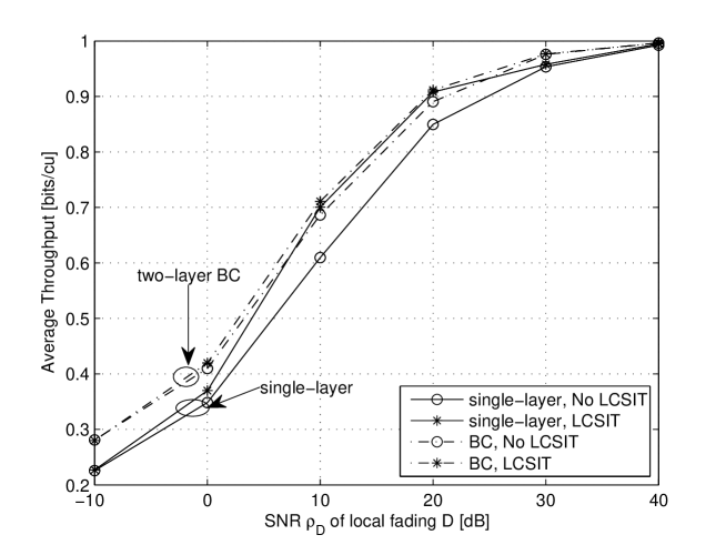
Figure 2: Average throughput $\eta$ versus the SNR $\rho_{D}$ with $T=2$, $C_{\max}=1$, $P=0\,\mathrm{dB}$, $\rho_{S}=0\,\mathrm{dB}$ and $K=0$.

In this section, we present numerical results to gain insights into the advantage of the proposed multi-layer HARQ strategies. In the figures, the cases with and without local CSI at the encoder are denoted by “LCSIT” and “No LCSIT”, respectively. We assume Rayleigh fading for the side information $Y_{t}$ and Rician fading for the signal $V_{t}$ received by the relay with Rician factor $K$ (i.e., $K$ is the ratio of the power of line-of-sight (LOS) component to that of non-LOS component). The rationale behind these distributions comes from the application to the cloud radio access scenario (see Sec. I), in which $Y_{t}$ is the signal received by out-of-cell BSs, which typically lack the direct LOS component, unlike the signal $V_{t}$ received by the in-cell BS. The signal-to-noise ratios (SNRs) of the source-to-relay and the source-to-destination links are defined as $\mathbb{E}[|D_{t}|^{2}]=\rho_{D}$ and $\mathbb{E}[|S_{t}|^{2}]=\rho_{S}$, respectively.

We first examine in Fig. 2 how the SNR $\rho_{D}$ of the relay fading channel $D$ affects the average throughput $\eta$ by plotting $\eta$ versus the SNR $\rho_{D}$ under the LTSC model with $T=2$, $C_{\max}=1$, $P=0\,\mathrm{dB}$, $\rho_{S}=0\,\mathrm{dB}$ and $K=0$. With local CSI at the encoder, the proposed BC scheme shows performance gain over the conventional single-layer approach only in the range of low SNR $\rho_{D}$. This is because in this case, BC is only used to combat the uncertainty of the fading gain $S_{t}$, whose relevance becomes less pronounced as $\rho_{D}$ increases. However, with no local CSI at the encoder, the gain of the BC remains substantial for all SNRs $\rho_{D}$, since in this case, the CSI uncertainty at the encoder includes both $D_{t}$ and $S_{t}$.

Figure 3: Average throughput $\eta$ versus the backhaul capacity $C_{\max}$ with $T=2$, $P=0\,\mathrm{dB}$, $\rho_{D}=\rho_{S}=0\,\mathrm{dB}$ and $K=0$.

In Fig. 3, we plot the throughput performance versus the backhaul capacity $C_{\max}$ for the LTSC model with $T=2$, $P=0\,\mathrm{dB}$, $\rho_{D}=\rho_{S}=0\,\mathrm{dB}$ and $K=0$. It is observed that the impact of the local CSI at the encoder becomes more significant for larger backhaul capacities $C_{\max}$, since the performance is more affected by the encoder-to-relay link if the backhaul capacity $C_{\max}$ is large enough. Moreover, the flexibility afforded by BC makes the effect of LCSIT less relevant than for conventional single-layer transmission.

Figure 4: Average throughput $\eta$ versus the maximum number $T$ of transmissions with $C_{\max}=1$, $P=0\,\mathrm{dB}$, $\rho_{D}=10\,\mathrm{dB}$, $\rho_{S}=0\,\mathrm{dB}$ and $K=0$.

In Fig. 4, we observe the effect of the maximum number $T$ of transmissions for the LTSC model with $C_{\max}=1$, $P=0\,\mathrm{dB}$, $\rho_{D}=10\,\mathrm{dB}$, $\rho_{S}=0\,\mathrm{dB}$ and $K=0$. For both cases with local CSI at the encoder or not, the advantage of the BC scheme diminishes as $T$ increases. This implies that the HARQ strategy is able to compensate for a large fraction of performance degradation of the single-layer scheme when enough number of transmissions are allowed. This trend is more apparent in the case with no local CSI at the encoder, due to the layer gains of BC.

Figure 5: Average throughput $\eta$ versus the factor $K$ of Rician fading with $C_{\max}=2$, $T=2$, $P=0\,\mathrm{dB}$ and $\rho_{D}=\rho_{S}=20\,\mathrm{dB}$.

In Fig. 5, we investigate the advantage of the adaptive compression scheme proposed in Sec. V by plotting the throughput performance versus the Rician factor $K$ for the LTSC with $C_{\max}=2$, $T=2$, $P=0\,\mathrm{dB}$ and $\rho_{D}=\rho_{S}=20\,\mathrm{dB}$. We recall that the adaptive compression was proposed to opportunistically leverage better fading states. In accordance with this motivation, the adaptive compression is observed to be advantageous as the factor $K$ grows due to increased frequency of good fading states that can be exploited via the proposed strategy.

Figure 6: Average throughput $\eta$ versus the SNRs $\rho_{D}=\rho_{S}$ with no local CSI at the encoder and $T=2$, $P=0\,\mathrm{dB}$, $C_{\max}=5$ and $K=0$.

Finally, in Fig. 6, we compare the average throughput performance under the LTSC and STSC models with no local CSI at the encoder and $T=2$, $P=0\,\mathrm{dB}$, $C_{\max}=5$ and $K=0$. With single-layer transmission, it is seen that the STSC model leads to better performance than LTSC due to the diversity gain. However, with BC, an additional factor determines the performance comparison, namely the possibility for “opportunistic retransmission” under LTSC. Specifically, under the LTSC model, when the encoder is reported an ACK for the first-layer message $M_{1}$, it can transmit the second layer $M_{2}$ in the next slot in order to leverage the good fading state. In contrast, under the STSC model, this is not possible since the fading coefficients $D_{t}$ and $S_{t}$ vary independently from block to block. From the figure, it is observed that this factor is dominant in the low-to-moderate SNR range, where the performance of BC transmission under the LTSC model is better than under the STSC model.

VIII Conclusions

Motivated by the uplink of cloud radio access networks, we have studied robust transmission and compression schemes for the fading relay channel with an out-of-band relay. Specifically, we have adopted a multi-layer BC transmission strategy coupled with HARQ, thus allowing for variable-length transmission and variable-rate decoding, under two different channel models, LTSC and STSC. Moreover, we have proposed an adaptive compression strategy at the relay that is able to leverage better fading state based on the HARQ feedback received from the destination. We have demonstrated the performance gain of the proposed schemes over conventional single-layer approaches via extensive simulations.

Appendix A Proof of Lemmas 1-3

In this Appendix, we derive the probabilities presented in Lemmas 1-3. Since we assumed the LTSC model (3) in Sec. IV, we have $D_{t}=D$ and $S_{t}=S$ for all $t=1,\ldots,T$. We first calculate the probabilities conditioned on $D=d$ and the results in Lemmas 1-3 are then obtained by taking expectation over $D$.

A-A Proof of Lemma 1

In this subsection, we compute the probability $p_{\mathrm{out}}^{1}(k)$ that the message $M_{1}$ is not decoded until slot $k$. Since we have assumed the IR-based HARQ approach, the probability $p_{\mathrm{out}}^{1}(k)$ can be calculated as the probability that the mutual information accumulated along the first $k$ slots is smaller than $R_{1}$ [13]:

$$p_{\mathrm{out}}^{1}(k) =\mathbb{E}_{D}\left[\Pr\left[k\cdot I(X_{1,t};\bar{Y}_{t}|\mathrm{BC\,mode})<R_{1}(D)|\,D\right]\right],$$ (47)

where the mutual information $I(X_{1,t};\bar{Y}_{t}|\mathrm{BC\,mode})$ is given as

$$I(X_{1,t};\bar{Y}_{t}|\mathrm{BC\,mode})=f_{\mathrm{I}}(\alpha(D)P,\bar{\alpha}(D)P,a_{D},S,D),$$ (48)

with the function $f_{\mathrm{I}}(P,\bar{P},a,s,d)$ defined in (40). If we express the probability (47) using the CDF of $S$, we arrive at the expression (17).

A-B Proof of Lemma 2

This subsection computes the probability $p_{\mathrm{out}}^{2}(k)$ that the message $M_{2}$ is not decoded until slot $k$. Using the total probability theorem, we can write the probability $p_{\mathrm{out}}^{2}(k)$ as

$$p_{\mathrm{out}}^{2}(k)= \sum_{l=1}^{k}\mathbb{E}_{D}\left[\Pr\left[\begin{array}[]{c}(l-1)\cdot I(X_{1,t};\bar{Y}_{t}|\mathrm{BC\,mode})<R_{1}(D)\leq l\cdot I(X_{1,t};\bar{Y}_{t}|\mathrm{BC\,mode}),\\ l\cdot I(X_{2,t};\bar{Y}_{t}|X_{1,t},\mathrm{BC\,mode})+(k-l)\cdot I(X_{2,t};\bar{Y}_{t}|X_{1,t},\mathrm{SL\,mode})<R_{2}\end{array}\Bigg{|}\,D\right]\right]$$ (51)

$$+p_{\mathrm{out}}^{1}(k),$$ (52)

where the probability $p_{\mathrm{out}}^{1}(k)$ was derived in the previous subsection and the mutual information quantities related to the second layer are given as

$$I(X_{2,t};\bar{Y}_{t}|X_{1,t},\mathrm{BC\,mode})= f_{\mathrm{I}}(\bar{\alpha}(D)P,\alpha P,a_{D},S,D),$$ (53)

$$I(X_{2,t};\bar{Y}_{t}|X_{1,t},\mathrm{SL\,mode})= f_{\mathrm{I}}(P,0,a_{D},S,D).$$ (54)

The term inside the summation in (52) is then derived as

$$\Pr\left[\begin{array}[]{c}(l-1)\cdot I(X_{1,t};\bar{Y}_{t}|\mathrm{BC\,mode})<R_{1}(D)\leq l\cdot I(X_{1,t};\bar{Y}_{t}|\mathrm{BC\,mode}),\\ l\cdot I(X_{2,t};\bar{Y}_{t}|X_{1,t},\mathrm{BC\,mode})+(k-l)\cdot I(X_{2,t};\bar{Y}_{t}|X_{1,t},\mathrm{SL\,mode})<R_{2}(D)\end{array}\Bigg{|}\,D\right]$$ (57)

$$= \Pr\left[\begin{array}[]{c}\left(1-2^{2R_{1}(D)/(l-1)}\bar{\alpha}(D)\right)b_{D}PS<(2^{2R_{1}(D)/(l-1)}-1)b_{D}+(2^{2R_{1}(D)/(l-1)}\bar{\alpha}(D)-1)Pa_{D},\\ (2^{2R_{1}(D)/l}-1)b_{D}+(2^{2R_{1}(D)/l}\bar{\alpha}(D)-1)Pa_{D}\leq(1-2^{2R_{1}(D)/l}\bar{\alpha}(D))b_{D}PS,\\ \left(b_{D}\left(1+\bar{\alpha}(D)PS\right)+\bar{\alpha}(D)Pa_{D}\right)^{l}\left(b_{D}(1+PS)+Pa_{D}\right)^{k-l}<2^{2R_{2}(D)}b_{D}^{k}\end{array}\Bigg{|}D\right],$$ (61)

where the last condition makes it difficult to express the probability in terms of the CDF of $S$. Following [17], we assume the low SNR condition $\bar{\alpha}(D)P\ll 1$ so that we have $1+\bar{\alpha}(D)PS\approx 1$ in the last condition of the probability (61). Then, the probability (61) is approximated as

$$\Pr\left[\begin{array}[]{c}(l-1)\cdot I(X_{1,t};\bar{Y}_{t}|\mathrm{BC\,mode})<R_{1}(D)\leq l\cdot I(X_{1,t};\bar{Y}_{t}|\mathrm{BC\,mode}),\\ l\cdot I(X_{2,t};\bar{Y}_{t}|X_{1,t},\mathrm{BC\,mode})+(k-l)\cdot I(X_{2,t};\bar{Y}_{t}|X_{1,t},\mathrm{SL\,mode})<R_{2}(D)\end{array}\Bigg{|}\,D\right]$$ (64)

$$\approx \left[F_{S}(v_{k,l}^{\mathrm{UB}}(D))-F_{S}(v_{k,l}^{\mathrm{LB}}(D))\right]^{+},$$ (65)

where $v_{k,l}^{\mathrm{UB}}(D)$ and $v_{k,l}^{\mathrm{LB}}(D)$ are defined in Lemma 2. If we substitute (65) into (52), the result in Lemma 2 is obtained.

A-C Proof of Lemma 3

In this subsection, we compute the probability $p_{\mathrm{dec}}^{2}(k)$ that the message $M_{2}$ is successfully decoded in slot $k$. Following similar arguments as above, we can write $p_{\mathrm{dec}}^{2}(k)$ as

$$p_{\mathrm{dec}}^{2}(k)$$

$$= \sum_{l=1}^{k-1}\mathbb{E}_{D}\left[\Pr\left[\begin{array}[]{c}(l-1)\cdot I(X_{1,t};\bar{Y}_{t}|\mathrm{BC\,mode})<R_{1}(D)\leq l\cdot I(X_{1,t};\bar{Y}_{t}|\mathrm{BC\,mode}),\\ l\cdot I(X_{2,t};\bar{Y}_{t}|X_{1,t},\mathrm{BC\,mode})+(k-1-l)\cdot I(X_{2,t};\bar{Y}_{t}|X_{1,t},\mathrm{SL\,mode})<R_{2}(D),\\ R_{2}(D)\leq l\cdot I(X_{2,t};\bar{Y}_{t}|X_{1,t},\mathrm{BC\,mode})+(k-l)\cdot I(X_{2,t};\bar{Y}_{t}|X_{1,t},\mathrm{SL\,mode})\end{array}\Bigg{|}\,D\right]\right]$$ (69)

$$+\mathbb{E}_{D}\left[\Pr\left[\begin{array}[]{c}(k-1)\cdot I(X_{1,t};\bar{Y}_{t}|\mathrm{BC\,mode})<R_{1}(D)\leq k\cdot I(X_{1,t};\bar{Y}_{t}|\mathrm{BC\,mode}),\\ R_{2}(D)\leq k\cdot I(X_{1,t};\bar{Y}_{t}|\mathrm{BC\,mode})\end{array}\Bigg{|}\,D\right]\right].$$ (72)

Moreover, under the low SNR condition $\bar{\alpha}P\ll 1$, the term inside the summation is approximated as

$$\Pr\left[\begin{array}[]{c}(l-1)\cdot I(X_{1,t};\bar{Y}_{t}|\mathrm{BC\,mode})<R_{1}(D)\leq l\cdot I(X_{1,t};\bar{Y}_{t}|\mathrm{BC\,mode}),\\ l\cdot I(X_{2,t};\bar{Y}_{t}|X_{1,t},\mathrm{BC\,mode})+(k-1-l)\cdot I(X_{2,t};\bar{Y}_{t}|X_{1,t},\mathrm{SL\,mode})<R_{2}(D),\\ R_{2}(D)\leq l\cdot I(X_{2,t};\bar{Y}_{t}|X_{1,t},\mathrm{BC\,mode})+(k-l)\cdot I(X_{2,t};\bar{Y}_{t}|X_{1,t},\mathrm{SL\,mode})\end{array}\Bigg{|}\,D\right]$$ (76)

$$\approx \left[F_{S}(u_{k,l}^{\mathrm{UB}}(D))-F_{S}(u_{k,l}^{\mathrm{LB}}(D))\right]^{+},$$ (77)

where we have defined $u_{k,l}^{\mathrm{UB}}(D)$ and $u_{k,l}^{\mathrm{LB}}(D)$ in Lemma 3. Moreover, we can derive the last term in (72) as

$$\Pr\left[\begin{array}[]{c}(k-1)\cdot I(X_{1,t};\bar{Y}_{t}|\mathrm{BC\,mode})<R_{1}(D)\leq k\cdot I(X_{1,t};\bar{Y}_{t}|\mathrm{BC\,mode}),\\ R_{2}(D)\leq k\cdot I(X_{1,t};\bar{Y}_{t}|\mathrm{BC\,mode})\end{array}\Bigg{|}\,D\right]$$ (80)

$$= \left[F_{S}(q_{k}^{\mathrm{UB}}(D))-F_{S}(q_{k}^{\mathrm{LB}}(D))\right]^{+},$$ (81)

with $q_{k}^{\mathrm{UB}}(D)$ and $q_{k}^{\mathrm{LB}}(D)$ defined in Lemma 3. As a result, we obtain (25) by plugging (77) and (81) into (72).

Appendix B Proof of Lemmas 4 and 5

In this appendix, we derive the results in Lemmas 4- 5 with adaptive compression.

B-A Proof of Lemma 4

If we assume the adaptive compression described in Sec. V, the probability $p_{\mathrm{out}}^{2}(k)$ is calculated as (52) with the mutual information $I(X_{2,t};\bar{Y}_{t}|X_{1,t},\mathrm{SL\,mode})$ changed from (54) to

$$I(X_{2,t};\bar{Y}_{t}|X_{1,t},\mathrm{SL\,mode})=f_{\mathrm{I}}(P,0,\hat{a}_{D},S,D).$$ (82)

The only difference from (54) is the improved compression gain $\hat{a}_{D}$. If we calculate (52) with (82), we immediately obtain the result in Lemma 4.

B-B Proof of Lemma 5

With the adaptive compression, the probability $p_{\mathrm{dec}}^{2}(k)$ is given as (72), and similar to the previous subsection, the only difference is that the mutual information $I(X_{2,t};\bar{Y}_{t}|X_{1,t},\mathrm{SL\,mode})$ is computed as (82) with the compression gain $\hat{a}_{D}$. Then, we can obtain the result in Lemma 5.

Appendix C Proof of Lemmas 6-8

In this appendix, we avoid repetition by focusing on the proof of (37) in Lemma 6 since the proof for Lemmas 7-8 follows similarly. With STSC, the probability $p_{\mathrm{out}}^{1}(2)$ is given as

$$p_{\mathrm{out}}^{1}(2)$$

$$= \Pr\left[I(X_{1,1};\bar{Y}_{1}|\mathrm{BC\,mode})+I(X_{1,2};\bar{Y}_{2}|\mathrm{BC\,mode})<R_{1}\right]$$

$$= \mathbb{E}_{D_{1},D_{2},S_{1}}\left[\Pr\left[\begin{array}[]{c}f_{\mathrm{I}}(\alpha(D)P,\bar{\alpha}(D)P,a_{D_{1}},S_{1},D_{1})+\\ f_{\mathrm{I}}(\alpha(D)P,\bar{\alpha}(D)P,a_{D_{2}},S_{2},D_{2})<R_{1}(D)\end{array}\Bigg{|}D_{1},D_{2},S_{1}\right]\right].$$ (85)

If we express the conditional probability inside the expectation in (85) with respect to the CDF of the fading coefficient $S_{2}$, we get Eq (37) in Lemma 6.

References

- [1] S. Liu, J. Wu, C. H. Koh and V. K. N. Lau, "A 25 Gb/s(/km2) urban wireless network beyond IMT-advanced," IEEE Comm. Mag., pp. 122-129, Feb. 2011.
- [2] P. Marsch, B. Raaf, A. Szufarska, P. Mogensen, H. Guan, M. Farber, S. Redana, K. Pedersen and T. Kolding, "Future mobile communication networks: challenges in the design and operation," IEEE Veh. Tech. Mag., vol. 7, no. 1, pp. 16-23, Mar. 2012.
- [3] A. Steiner and S. Shamai (Shitz), "Single-user broadcasting protocols over a two-hop relay fading channel," IEEE Trans. Inf. Theory, vol. 52, no. 11, pp. 4821-4838, Nov. 2006.
- [4] V. Pourahmadi, A. Bayesteh and A. K. Khandani, "Multilayer coding over multihop single-user networks," IEEE Trans. Inf. Theory, vol. 58, no. 8, pp. 5323-5337, Aug. 2012.
- [5] A. del Coso and S. Simoens, "Distributed compression for MIMO coordinated networks with a backhaul constraint," IEEE Trans. Wireless Comm., vol. 8, no. 9, pp. 4698-4709, Sep. 2009.
- [6] G. Chechik, A. Globerson, N. Tishby and Y. Weiss, "Information bottleneck for Gaussian variables," Jour. Machine Learn., Res. 6, pp. 165-188, 2005.
- [7] C. Tian and J. Chen, "Remote vector Gaussian source coding with decoder side information," IEEE Trans. Inf. Theory, vol. 55, no. 10, pp. 4676-4680, Oct. 2009.
- [8] L. Zhou and W. Yu, "Uplink multicell processing with limited backhaul via successive interference cancellation," in Proc. IEEE Glob. Comm. Conf. (Globecom 2012), Anaheim, CA, Dec. 2012.
- [9] C. T. K. Ng, C. Tian, A. J. Goldsmith and S. Shamai (Shitz), "Minimum expected distortion in Gaussian source coding with fading side information," IEEE Trans. Inf. Theory, vol. 58, no. 9, pp. 5725-5739, Sep. 2012.
- [10] S.-H. Park, O. Simeone, O. Sahin and S. Shamai (Shitz), "Robust and efficient distributed compression for cloud radio access networks," IEEE Trans. Veh. Tech., vol. 62, no. 2, pp. 692-703, Feb. 2013.
- [11] S.-H. Park, O. Simeone, O. Sahin and S. Shamai (Shitz), "Robust layered transmission and compression for distributed uplink reception in cloud radio access networks," submitted to IEEE Trans. Veh. Tech.
- [12] S.-H. Park, O. Simeone, O. Sahin and S. Shamai (Shitz), "Delay-tolerant robust communication on an out-of-band relay channel with fading side information," submitted to IEEE Int. Sym. Personal Ind. Mob. Radio Comm. (PIMRC 2013).
- [13] G. Caire and D. Tuninetti, "The throughput of hybrid-ARQ protocols for the Gaussian collision channel," IEEE Trans. Inf. Theory, vol. 47, no. 5, pp. 1971-1988, Jul. 2001.
- [14] T. M. Cover, "Comments on broadcast channels," IEEE Trans. Inf. Theory, vol. 44, no. 6, pp. 2524-2530, Oct. 1998.
- [15] S. Shamai (Shitz) and A. Steiner, "A broadcast approach for a single-user slowly fading MIMO channel," IEEE Trans. Inf. Theory, vol. 49, no. 10, pp. 2617-2635, Oct. 2003.
- [16] S. Verd and S. Shamai (Shitz), "Variable-rate channel capacity," IEEE Trans. Inf. Theory, vol. 56, no. 6, pp. 2651-2667, Jun. 2010.
- [17] A. Steiner and S. Shamai (Shitz), "Multi-layer broadcasting hybrid-ARQ strategies for block fading channels," IEEE Trans. Wireless Comm., vol. 7, no. 7, pp. 2640-2650, Jul. 2008.
- [18] A. E. Gamal and Y.-H. Kim, Network information theory. Cambridge University Press, 2011.
- [19] M. Zorzi and R. R. Rao, "On the use of renewal theory in the theory in the analysis of ARQ protocols," IEEE Trans. Comm., vol. 44, no. 9, pp. 1077-1081, Sep. 1996.
- [20] D. Bertsekas, Nonlinear programming. New York: Athena Scientific, 1995.