Zeros of the partition function and phase transition

Abstract

The equation of state of a system at equilibrium may be derived from the canonical or the grand canonical partition function. The former is a function of temperature $T$, while the latter also depends on the chemical potential $\mu$ for diffusive equilibrium. In the literature, often the variables $\beta=(k_{B}T)^{-1}$ and fugacity $z=\exp(\beta\mu)$ are used instead. For real $\beta$ and $z$, the partition functions are always positive, being sums of positive terms. Following Lee, Yang and Fisher, we point out that valuable information about the system may be gleaned by examining the zeros of the grand partition function in the complex $z$ plane (real $\beta$), or of the canonical partition function in the complex $\beta$ plane. In case there is a phase transition, these zeros close in on the real axis in the thermodynamic limit. Examples are given from the van der Waal gas, and from the ideal Bose gas, where we show that even for a finite system with a small number of particles, the method is useful.

I Introduction

In a senior level undergraduate or a beginning graduate course, examples of phase transition are often given from the classical van der Waals equation of state, and at a quantum level, from the Bose-Einstein condensation (BEC) of an ideal Bose gas.Landau and Lifshitz (1958); Huang (1965a) The treatment, naturally, focuses on the equation of state of the system as a function of physical parameters like the temperature $T$ and chemical potential $\mu$, which are real. It is instructive to learn, however, that the approach towards phase transition may be studied by examining the analytical behavior of the partition function for complex values of the parameters, even for a finite system where there is no discontinuity in the derivatives of the free energy.

For a system in thermal and diffusive equilibrium, it is convenient to calculate the ensemble average using the grand canonical partition function ${\cal Z}(\beta,z)$, where $\beta=(k_{B}T)^{-1}$, $k_{B}$ being the Boltzmann constant and $z=\exp(\beta\mu)$ the fugacity. Note that there is an implicit volume dependence in ${\cal Z}$, since the eigenenergies are volume dependent. We suppress this in our notation ${\cal Z}(\beta,z)$ for simplicity. The grand canonical partition function is a sum of positive definite terms for real positive values of $\beta$ and $z$, and as such cannot have a zero in the physical domain of these variables. Lee and YangYang and Lee (1952); Lee and Yang (1952) considered a lattice gas with a hard core interaction. Because of the short-range repulsion between the particles, only a finite number of particles may be packed into a finite volume. As we shall see, this allows one to express ${\cal Z}$ as a finite-degree polynomial in fugacity $z$. This polynomial is then completely defined in terms of its zeros on the complex fugacity plane. These zeros are all complex, coming in complex conjugate pairs. In the thermodynamic limit, the zeros coalesce in continuous lines, tending to pinch the positive real $z$ axis at a phase transition. In this paper, we show that this tendency sets in even at finite particle number and volume, with the zeros moving closer to the real axis as the particle number is increased. Even though complex, the closer a zero comes to the real axis, the more it dominates real thermodynamic properties. Note that the validity of the Lee-Yang method rests on the repulsive core between the particles.

Fisher Fisher (1965) pointed out that the zeros of the canonical partition function $Z_{N}(\beta)$ on the complex $\beta$ plane have an analogous behavior. However, Fisher zeros can give useful information even in the absence of the repulsive core. The Fisher zeros for ideal trapped bosons were studied in the context of BEC by Mülken et al.Mülken et al. (2001) In this paper, following the work of Hemmer et al.,Hemmer et al. (1966) we study the Lee-Yang zeros of the classical van der Waals gas (that has a phase transition with a critical temperature) and compare it with a Calogero gasCalogero (1969a); *calogero69a; Sutherland (1971a); *sutherland71a (that has no phase transition). The ideal Bose gas (which undergoes a phase transition at BEC) is studied in some detail, both using the grand canonical and the canonical formalisms. The heat capacity per particle in the grand canonical and canonical ensembles are compared at BEC to check how close these are for finite particle number. Since there is no short-range repulsion in the ideal Bose gas, the Lee-Yang zeros are not meaningful, but the Fisher zeros are. Accordingly, we find the pattern of these on the complex $\beta$ plane for 50 and 100 atoms. Even for such small number of particles, we see a clear tendency for the zeros to close in on the real $\beta$ axis. The calculations are done for the exact $Z_{N}(\beta)$ as well as the more commonly used continuous density of states. This will be discussed after the patterns of zeros are presented. The grand partition function, on the other hand, is shown to have a pole at phase transition for real $z=1$. Ikeda (1982); Wang and Kim (1999) A nontrivial modification over the ideal gas will be to introduce interparticle interaction through virial coefficients in the grand potential,Bhaduri et al. (2012) and study how the zeros of the grand canonical partition function shift on the complex plane. This is beyond the scope of the present paper.

II Partition Function

The canonical partition function (for fixed $N$) is defined as

$$Z_{N}(\beta)=\sum_{E_{i}^{(N)}}\exp(-\beta E_{i}^{(N)})~{},$$ (1)

where $E_{i}^{(N)}$ are the complete set of eigenenergies of the $N$-body system including states in the continuum, if any. The sum is taken over all states ${i}$ including the degeneracies. Since the energies $E_{i}^{(N)}$ depend on the volume of the system, there is a volume dependence in $Z_{N}(\beta)$. The grand canonical partition function, on the other hand, allows for particle exchange (in addition to energy) via the reservoir, and is defined as

$${\cal Z}(\beta,z)=\sum_{N=0}^{\infty}\sum_{E_{i}^{(N)}}\exp(-\beta E_{i}^{(N)}+\beta\mu N)~{}=\sum_{N=0}^{\infty}Z_{N}(\beta)z^{N}~{},$$ (2)

where the fugacity $z=\exp(\beta\mu)$. The simplest example is an ideal classical gas in a volume $V$. The $N$-particle canonical partition function is the $N$th power of the one-particle partition function $Z_{1}(\beta)$. The latter is calculated by integrating $\exp(-p^{2}/2m)$ over the phase space divided by $h^{3}$, where $h$ is the Planck’s constant. The net result is

$$Z_{N}(\beta)=\frac{1}{N!}~{}\left(\frac{V}{\lambda_{T}^{3}}\right)^{N}~{},$$ (3)

where $\displaystyle\lambda_{T}=\sqrt{\frac{2\pi\hbar^{2}}{Mk_{b}T}}$ is the thermal wave length, and the customary division by $N!$ has been made to preserve the extensive property of the entropy. By substituting Eq. (3) in Eq. (2), we obtain

$$\frac{1}{V}\ln{\cal Z}^{(0)}(\beta,z)=\frac{z}{\lambda_{T}^{3}}~{},$$ (4)

where the superscript on ${\cal Z}$ denotes a non-interacting system.

More generally, for an interacting gas with short-range interparticle repulsion, Eq. (2) shows that ${\cal Z}$ is a finite degree polynomial in $z$, and therefore may be completely defined in terms of its zeros. These zeros, however, cannot be on the real positive $z$-axis, since every term in Eq. (2) is then positive. Accordingly, for complex $z$ (but real positive $\beta$), Eq. (4) may be generalized to Fisher (1965)

$${\cal Z}(\beta,z)=\prod_{r}\left(1-\frac{z}{z_{r}}\right)~{}.$$ (5)

The zeros $z_{r}(\beta,V)$ come in complex conjugate pairs since the coefficients $Z_{N}(\beta)$ of the polynomial (2) are real. In case there is a phase transition at some temperature, a zero and its complex conjugate tend to pinch the real $z$ axis. If there are more than one phase transitions, there are segments on the real positive $z$-axis that are zero-free. The grand potential $\Omega=-k_{B}T\ln{\cal Z}(\beta,z)=-PV$, hence $\displaystyle\beta P=\frac{1}{V}\ln{\cal Z}(z,\beta)$. Yang and Lee Yang and Lee (1952) proved in general that for $V\rightarrow\infty$, this limit exists, and $P$ increases monotonically in the zero-free segments. At the interface of two phases, the pressure $P$ remains continuous, but its slope as a function of $\ln z$ is not the same. Moreover, in the thermodynamic limit, the number density $\rho=\frac{\textstyle\partial}{\textstyle\partial\ln z}(\beta P)$ may be discontinuous as a function of $\ln z$ in the interface of two phases (see Finkelstein.*[][; chapter10.]finkelstein69)

For our example in the next section, it is more relevant to take a finite volume $V$ which contains $N$ particles. If there is a hard-core repulsion, then there is a maximum number $N_{\mathrm{max}}$ that can be accommodated in this volume. Then the infinite upper limit in the sum over $N$ in Eq. (2) is replaced by $N_{\mathrm{max}}$, and ${\cal Z}(\beta,z)$ is a polynomial of order $N_{\mathrm{max}}$.

II.1 van der Waals gas

This is a classical example, studied in the context of Yang-Lee zeros by Hemmer et al. Hemmer et al. (1966) Equation (2) is used with the canonical partition function that is postulated to be

$$Z_{N}(\beta)=\frac{1}{N!}(V-Nb)^{N}~{}\exp\left(\frac{2a\beta}{V}\frac{N(N-1)}{2}\right)~{},$$ (6)

where $b$ is interpreted as the volume associated with the repulsive core, and $a$ as a measure of the outer attraction. For calculating ${\cal Z}(\beta,z)$ using Eq. (2), one takes $N_{\mathrm{max}}=V/b$. Note that the excluded volume effect, and the outer pair-wise attraction are both incorporated in the canonical $Z_{N}(\beta)$ above. The equation of state can easily be deduced from the postulated $Z_{N}(\beta)$. One obtains the Helmholtz free energy $F=-1/\beta\ln Z_{N}(\beta)$, and the pressure $\displaystyle P=-\left(\frac{\partial F}{\partial V}\right)_{T}$. A little algebra then yields the equation of state

$$\left(P+\frac{N^{2}}{V^{2}}a\right)(V-Nb)=Nk_{B}T~{}.$$ (7)

where we have assumed $N\gg 1$. One makes the Maxwell construction across the unphysical region in which $P$ decreases with $V$ to obtain the equation of state. The critical point is obtained by additionally imposing the condition that the first and second partial derivatives of $P$ with respect to $V$ (at constant temperature ) are zero; see for example Landau and Lifshitz.Landau and Lifshitz (1958) The critical temperature is given by

$\begin{array}[]{c@{\hspace{0.0in}}c@{\hspace{0.0in}}c}\leavevmode\resizebox{166.2212pt}{}{\includegraphics[angle={270}]{fig_1a.eps}}&\leavevmode\resizebox{166.2212pt}{}{\includegraphics[angle={270}]{fig_1b.eps}}&\leavevmode\resizebox{166.2212pt}{}{\includegraphics[angle={270}]{fig_1c.eps}}\end{array}$

Figure 1: The Yang-Lee zeros of the grand partition function for a van der Waals system of 40 particles, i.e., $V=40$, $d=1$, $N=40$. From left to right the patterns correspond to $\nu=2$, $\nu=27/8$, and $\nu=4$.

$$k_{B}T_{c}=\frac{8}{27}\frac{a}{b}~{}.$$ (8)

inline](Programs: /home/vandijk/2013/paper_LY_zeros/van_der_Waal/maple/V_30_nu_?.eps.) Our interest here is to compute the zeros of ${\cal Z}(\beta,z)$ using Eqs. (2) and (6) in the complex $z$-plane for real values of $T$. From Eq. (6), we see that there is a cut-off in the upper limit of the summation over $N=N_{\mathrm{max}}=V/b$, which prevents us from obtaining ${\cal Z}$ analytically. Note, from Eq. (8), that $a/b$ has the dimension of energy. Setting $a=\nu k_{B}T$, and $b=1$, Eq. (8) takes the form

$$\nu=\frac{27}{8}\frac{T_{c}}{T}$$ (9)

For our calculations, we take $N_{\mathrm{max}}=V/b=40$. In Fig. 1, we plot the zeros of ${\cal Z}(T,z)$ for three choices of $\nu$, corresponding to $T>T_{c},T=T_{c},$ and $T<T_{c}$. Even for $N_{\mathrm{max}}=40$, we clearly see the zeros closing in on the real $z$-axis for $T\leq T_{c}$. system of 40 particles, i.e., $V=40$, $d=1$, $N=40$. From left to right the inline](Programs: /home/vandijk/2013/paper_LY_zeros/van_der_Waal/maple/V_30_nu_?.eps.)

II.2 Calogero gas

The Calogero gas is an exactly solvable one-dimensional model where point particles are interacting with a pair-wise inverse-square potential.Calogero (1969a); *calogero69a; Sutherland (1971a); *sutherland71a The particles are trapped in a harmonic oscillator (HO) potential. For a repulsive interaction, the high temperature limit of the canonical partition function is given byBhaduri et al. (2010) ($\hbar=1$)

$$Z_{N}(\beta)=\frac{1}{N!}\frac{1}{(\beta\omega)^{N}}\exp\big{(}-\alpha\beta\omega N(N-1)/2\big{)}~{},$$ (10)

where $\omega$ is the oscillator frequency, and $\alpha$ is a measure of the strength of the inverse-square two-body potential. Since the density of states is a constant in a one-dimensional HO, it is like a two-dimensional gas. The oscillator length is $l=\sqrt{\hbar/M\omega}$, and we may define a density $n=N/l^{2}=N\omega$, with $\hbar=M=1$. The thermodynamic limit is taken as $N\rightarrow\infty,\ \omega\rightarrow 0$, with $N\omega=n$ a constant. For $N\gg 1$, we then get

$$Z_{N}(\beta)=\frac{1}{N!}\frac{1}{(\beta\omega)^{N}}\exp(-\alpha\beta nN/2)~{}.$$ (11)

With this $Z_{N}(\beta)$, the grand partition function ${\cal Z}(\beta,z)$ may be obtained analytically by summing over all $N\rightarrow\infty$ . This is so because these are point particles with no excluded volume. A little algebra immediately gives

$$\ln{\cal Z}(\beta,z)=\frac{z}{\beta\omega}\exp(-n\alpha\beta/2).$$ (12)

This is of the same form as Eq. (4) of the perfect classical gas, monotonically increasing with $z$. There is, of course, no phase transition.

III Ideal Trapped Bosons and BEC

Quantum effects are manifest in a gas when the de Broglie thermal wavelength of a particle is larger than, or of the order of, the average interparticle spacing. BEC was first experimentally realized when neutral ⁸⁷Rb atomsAnderson et al. (1995) and ²³Na atomsDavis et al. (1995) were magnetically trapped in a HO potential at a few hundred degrees nano-Kelvin. For a large number of identical bosons, a sizable fraction of them abruptly start occupying the lowest level even at a temperature much, much larger than the energy spacing $\hbar\omega$. This is the condensation temperature. We follow the treatment of Ketterle and van Druten Ketterle and van Druten (1996) to find the behaviour of the chemical potential $\mu$ as the temperature is lowered. Here both the temperature and chemical potential are taken to be real. Consider $N$ ideal bosons in the grand canonical ensemble occupying a discrete spectrum of single-particle states with energies $\varepsilon_{n}$ at temperature $T$. Its grand partition function may be written as*[][; page199.]huang65a

$${\cal Z}(\beta,z)=\prod_{n}\left(1-z\exp(-\beta\varepsilon_{n})\right)^{-1}$$ (13)

We then get

$$\begin{split}\langle N\rangle&=z\frac{\partial}{\partial z}\ln{\cal Z}=\sum_{n=0}^{\infty}\dfrac{e^{\textstyle-\beta(\varepsilon_{n}-\mu)}}{1-e^{\textstyle-\beta(\varepsilon_{n}-\mu)}}\\ &=\sum_{n=0}^{\infty}\sum_{l=1}^{\infty}e^{\textstyle-\beta l\varepsilon_{n}}z^{l}=\sum_{l=1}^{\infty}z^{l}Z_{1}(l\beta),\end{split}$$ (14)

where $Z_{1}(\beta)$ is the exact one-particle partition function and $z=e^{\textstyle\beta\mu}$. Since the occupancy factor of a state has to be positive, it follows from the first term on the RHS that the smallest value $\mu$ can take is $\varepsilon_{0}$, the lowest energy single-particle state. In the following, we choose $\varepsilon_{0}=0$, so that $z\leq 1$, and the power series in $z$ does not involve large numbers. Up till now the formulae are general. We now specialize to a shifted harmonic oscillator energy spectrum, which in one dimension is given by $n\hbar\omega$, with $n$ going from zero to $\infty$. For an isotropic three-dimensional harmonic oscillator $Z^{(3d)}_{1}(\beta)=\left(Z_{1}^{(1d)}(\beta)\right)^{3}$. Thus we write for the three-dimensional HO

$$\langle N\rangle=\sum_{l=1}^{\infty}z^{l}\left(Z_{1}^{(1d)}(l\beta)\right)^{3}.$$ (15)

Note that with the choice of zero-energy ground state, $Z_{1}^{(1d)}(\beta)=1/(1-\exp(-\beta\omega))$. In Fig. 2, we plot the variation

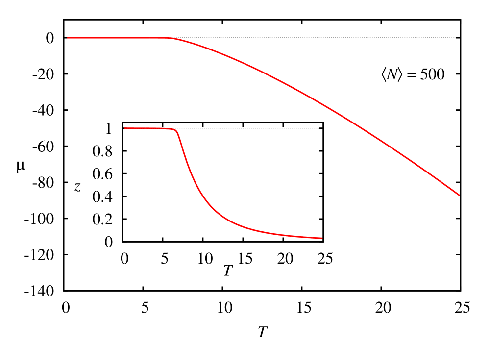
Figure 2: The chemical potential $\mu$ and the fugacity $z$ as a function of temperature $T$ when $\varepsilon_{0}=0$ for a system of bosons in a three-dimensional HO with $\langle N\rangle=500$. inline](Program: /home/vandijk/2012/zeros/Lee-Yang/december_11/z_mu_vs_T_qp.f).

of the chemical potential and the fugacity as a function of $T$ for a system of trapped bosons in a three dimensional isotropic harmonic oscillator when $\langle N\rangle=500$ (we have set $\omega=1$). Note that the constraint on $\langle N\rangle$ makes $\mu$, and therefore $z$ temperature dependent. There is no discontinuity in $\mu$ or $z$ for a finite number of particles, but there is a hint of rapid turning to a plateau in both cases near $T=7$. This gets more pronounced as $\langle N\rangle$ gets larger. Similarly we can calculate the average energy in the grand canonical ensemble,

$$\langle E\rangle=\sum_{n}\frac{\varepsilon_{n}}{e^{\textstyle\beta(\varepsilon_{n}-\mu)}-1}=-\sum_{l=1}^{\infty}\frac{z^{l}}{l}\frac{\partial}{\partial\beta}Z_{1}(\beta l)$$ (16)

For later use, we write the following expression for $\ln{\cal Z}(\beta,z)$ from Eq. (13),

$$\ln{\cal Z}(\beta,z)=-\sum_{n}\ln(1-z\exp(-\beta\varepsilon_{n}))$$ (17)

Noting that $\displaystyle\ln(1-x)=-\sum_{l=1}^{\infty}\dfrac{x^{l}}{l}$, a few steps give

$$\ln{\cal Z}(\beta,z)=\sum_{l=1}^{\infty}\frac{z^{l}}{l}Z_{1}(l\beta)~{}.$$ (18)

where

$$Z_{1}(l\beta)=(1-\exp(-l\beta))^{-3}.$$ (19)

The derivative of $\langle E\rangle$ with respect to $T$ gives the heat capacity.

In Fig. 3, the heat capacity per particle at constant $\omega$ is shown for $\langle N\rangle=500$ and $\langle N\rangle=50$ based on the grand partition analysis of this section.

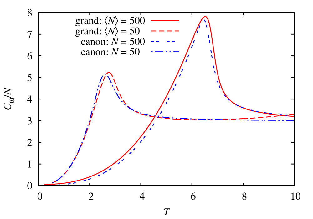
Figure 3: The heat capacity per particle for a system of trapped bosons as a function of temperature. The calculations based on the grand partition function, i.e., Eq. (16), are labelled “grand”. The graphs labelled “canon” are based on the canonical partition function discussed later. inline]The graph grand: $N=50$ seems to be correct. One needs to explain why as $T$ becomes large the specific heat increases. In my program, I started with $N=500$ and slowly decreased $N$. As $N$ gets smaller to 100 say, then the specific heat per particle begins to increase as $T$ increases. It is noticeable on the graph for $N=50$.

Next we shall compare these results with the canonical formalism, which requires knowledge of $Z_{N}(\beta)$. For finite $N$ and $\langle N\rangle$, the canonical and grand canonical ensembles may yield different results.

Before concluding this section, we note that for ideal bosons, in the thermodynamic limit, there is an analytical simple pole at $z=1$, the condensation point. This may be seen from Eq. (13), which shows that there are poles at

$$z_{n}=\exp(\beta\epsilon_{n}).$$ (20)

With our choice of $\epsilon_{n}\geq 0$, the RHS above is $\geq 1$. But as the inset of Fig. 2 shows, physically allowed $z\leq 1$. Therefore from Eq. (20), the only pole in the physical region is at $z=1$.

$\begin{array}[]{c@{\hspace{0.0in}}c@{\hspace{0.0in}}}\leavevmode\resizebox{252.94499pt}{}{\includegraphics[angle={-90}]{fig_4a.eps}}&\leavevmode\resizebox{252.94499pt}{}{\includegraphics[angle={-90}]{fig_4b.eps}}\end{array}$

Figure 4: The Fisher zeros for a systems of 50 or 100 trapped bosons taking into account the exact discrete energy spectrum.

III.1 Calculation of $Z_{N}(\beta)$

In order to obtain the grand partition function ${\cal Z}(\beta,z)$ from Eq. (2), we need to calculate the canonical partition function $Z_{N}(\beta)$. As we shall see soon, the zeros of the canonical partition function on the complex $\beta$ plane (called the Fisher zeros) are interesting in their own right. For an ideal boson or fermion gas, $Z_{N}(\beta)$ may be obtained from $Z_{1}(\beta)$ using a recursion relation.Borrmann and Franke (1993) We give an outline of the derivation of this important relation for ideal bosons. We start with the relation (18). On further expanding the exponential in a power series, and equating power by power to the series given by Eq. (2),

$${\cal Z}(\beta,z)=1+zZ_{1}(\beta)+z^{2}Z_{2}(\beta)+z^{3}Z_{3}(\beta)+\dots,$$ (21)

the desired recursion relation emerges, which for bosons is given by Borrmann and Franke (1993)

$$Z_{N}(\beta)=\frac{1}{N}\sum_{n=1}^{N}Z_{1}(n\beta)Z_{N-n}(\beta).$$ (22)

It is now straightforward to obtain $\displaystyle\langle E\rangle=-\frac{\partial}{\partial\beta}\ln Z_{N}(\beta)$, and its derivative with respect to $T$ to obtain the heat capacity. In Fig. 3 we plot $\displaystyle\dfrac{C_{\omega}}{N}=\dfrac{1}{N}\dfrac{\partial\langle E\rangle}{\partial T}$ as the graphs labelled “canon”.

III.2 Fisher zeros for ideal bosons

Fisher pointed out that there are complex zeros of the canonical partition function $Z_{N}(\beta)$ on the complex $\beta$ plane. For a fixed $N$, the number of zeros on the complex plane, denoted by $\beta_{r}$, is finite. Therefore $Z_{N}(\beta)$ may be expressed as a finite product $\prod{\left(1-\frac{\textstyle\beta}{\textstyle\beta_{r}}\right)}$. This is unlike the Lee-Yang zeros whose validity was contingent on short-range interparticle repulsion. At a phase transition, the complex Fisher zeros close in on the real $\beta$ axis. The Helmholtz free energy for an $N$-particle system is given by $\displaystyle F=-\dfrac{1}{\beta}\ln Z_{N}(\beta)$. Since $Z_{N}(\beta)$ is a sum of exponential positive terms in $\beta$, and is larger than unity (the contribution of the state at $\varepsilon=0$ ), $F$ does not change sign, and always remains negative. Nevertheless, $Z_{N}(\beta)$ is an entire function of $\beta$ in the complex plane. For trapped bosons in a $3$-dimensional HO, we may use the exact $Z_{1}(\beta)$ given by Eq. (19). Then, using the recursion relation (22), $Z_{N}(\beta)$ is a polynomial in the variable $y=e^{\textstyle-\beta}$ in this example of a $3$-dimensional HO.Schmidt and Schnack (1999) (See Appendix A.) The exact form of $Z_{1}(\beta)$ is taken, but whether $\varepsilon_{0}=3/2$ or $\varepsilon_{0}=0$ the zeros occur at the same positions in the complex $\beta$ plane. Only a small fraction of the zeros are shown in the Fig. 4. noline]Obtain a similar graph when $\varepsilon_{0}=0$. (Done.)

Even for $N=50$, there is a tendency for the zeros to approach the real $\beta$-axis, but clearly the system is not condensed. We also display the plot of zeros for $N=100$ ideal bosons. Calculations are much easier if one uses $Z_{1}(\beta)=1/\beta^{3}$, which is the leading term of the exact Eq. (19). This corresponds to a continuous single-particle density of states that grows quadratically. In Fig. 5, we show the pattern of complex zeros of the corresponding

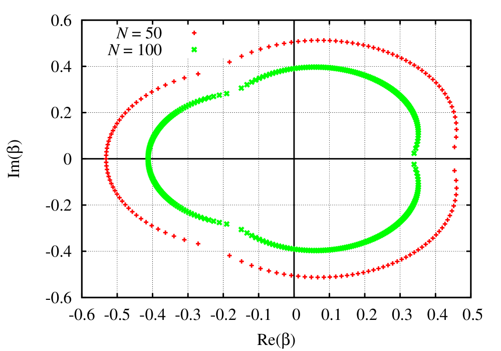
Figure 5: The Fisher zeros for systems of 50 or 100 trapped bosons with a continuous energy distribution.

$Z_{N}(\beta)$ for $N=50$ and $N=100$. Comparison with Fig. 4 shows considerable difference: the number of zeros being much smaller for the case of continuous density of states. In the latter, $\beta_{c}$ is about $10$ percent higher. In both, the estimated condensation temperaure $T_{c}$ increases approximately as $N^{1/3}$.

IV Concluding Remarks

We have shown that the advent of a phase transition in a system is reflected in the pattern of the complex zeros of the partition function. Strictly speaking, a phase transition takes place only in the thermodynamic limit. But even for a finite system with relatively small number of particles, the pattern of complex zeros begin to close in on the real fugacity or inverse temperature axis. For the grand partition function Lee-Yang zeros, it is imperative to have short-range repulsion in the interparticle interaction, whereas for the Fisher zeros of the canonical partition function, this is not necessary. In the case of BEC, a signal of a phase transition is a peak in the heat capacity per particle on the real temperature axis, as shown in Fig. 3. This peak shows up nicely even for $\langle N\rangle=50$. In Fig. 4, the complex Fisher zeros for $N=50$ appear to close in on the real axis at the same temperature. The Lee-Yang zeros in the van der Waal gas seem to close in towards the real z axis for $T\leq T_{c}$. Finally, we note that even though there are no Lee-Yang zeros for the ideal Bose gas, the grand canonical partition function has a simple pole at $z=1$, which was already noticed by Kastura.Katsura (1963)

Appendix A Fisher zeros

The Fisher zeros are the zeros of the $N$-particle canonical partition function $Z_{N}(\beta)$ in the complex $\beta$ plane. Given $Z_{0}(\beta)=1$ and $Z_{1}(\beta)=\sum_{n=0}^{\infty}e^{\textstyle-\beta E_{n}}$, we can obtain $Z_{N}(\beta)$ by the recursionBorrmann and Franke (1993)

$$Z_{N}(\beta)=\dfrac{1}{N}\sum_{k=1}^{N}Z_{1}(k\beta)Z_{N-k}(\beta).$$ (23)

If $Z_{1}(\beta)$ is the canonical partition function of a single particle in a three-dimensional harmonic oscillator well, then

$$Z_{1}(\beta)=\left(\sum_{n=0}^{\infty}e^{\displaystyle-\beta\varepsilon_{n}}\right)^{3}=\left(\dfrac{e^{\textstyle-\beta\hbar\omega/2}}{1-e^{\textstyle-\beta\hbar\omega}}\right)^{3}.$$ (24)

where $\varepsilon_{n}=(n+1/2)\hbar\omega$. The calculation of $Z_{N}(\beta)$ can be simplified by introducing Schmidt and Schnack (1999) $y=e^{\textstyle-\beta\hbar\omega}$ so that

$$Z_{N}(y)=\dfrac{y^{3N/2}}{\prod_{j=1}^{N}(1-y^{j})^{3}}P_{N}(y).$$ (25)

The recursion relation (23) is reformulated as $P_{0}(y)=P_{1}(y)=1$ and

$$P_{N}(y)=\dfrac{1}{N}\sum_{k=1}^{N}\dfrac{\prod_{j=N-k+1}^{N}(1-y^{j})^{3}}{(1-y^{k})^{3}}P_{N-k}(y).$$ (26)

The $P_{N}(y)$ is a polynomial in $y$ and when it is zero so is $Z_{N}(y)$. In the case that $\varepsilon_{n}=n\hbar\omega$ rather than $(n+1/2)\hbar\omega$ we have

$$Z_{1}(y)=\dfrac{1}{(1-y)^{3}},\ \ \ Z_{N}(y)=\dfrac{1}{\prod_{j=1}^{N}(1-y^{j})^{3}}P_{N}(y),$$ (27)

where the $P_{N}$ satisfy the same recursion (26). Thus the Fisher zeros will be the same irrespective of $\varepsilon_{0}=0$ or $\hbar\omega/2$.

Since $P_{N}(y)$ is a polynomial the number of zeros is equal to its degree which increases rapidly with particle number. For example, for $N=50$ there are 3495 zeros. We determine a subset to give a clear indication that the pattern of zeros pinches the positive real $\beta$ axis.

In order to numerically obtain the zeros we use the Laguerre method since this method “is guaranteed to converge to a (zero) from any starting point.” *[][; pages263ff.]press_F86 Once a zero is found we deflate the polynomial to obtain a second distinct zero and repeat. For larger $N$ the zeros may be close together so we check the accuracy of the zero $y_{0}$ by considering a small circle centred on $y_{0}$ in the complex $y$ plane and by ensuring that the curves $\mathrm{Re}(P_{N}(y))=0$ and $\mathrm{Im}(P_{N}(y))=0$ intersect inside the small disc. By using a radius of say $10^{-5}$ we have an estimate of the precision of the zero. Since we are interested in zeros that pinch the positive real $\beta$ axis, we limit the variable $y$ so that $|y|<1$ which results in $\mathrm{Re}(\beta)>0$.

References

- Landau and Lifshitz (1958) L. D. Landau and E. M. Lifshitz, Statistical physics (Addison-Wesley, Reading, Mass., USA, 1958).
- Huang (1965a) Kerson Huang, Statistical mechanics (John Wiley, New York, 1965).
- Yang and Lee (1952) C. N. Yang and T. D. Lee, “Statistical theory of equations of state and phase transitions. I. Theory of condensation,” Phys. Rev. 87, 404–409 (1952).
- Lee and Yang (1952) T. D. Lee and C. N. Yang, “Statistical theory of equations of state and phase transitions. II. Lattice gas and Ising model,” Phys. Rev. 87, 410–419 (1952).
- Fisher (1965) Michael E. Fisher, “The nature of critical points,” in Lectures in theoretical physics, Vol. 7C, edited by W.E. Britten (University of Colorado Press, Boulder, Colorado, USA, 1965) pp. 1–159.
- Mülken et al. (2001) Oliver Mülken, Peter Borrmann, Jens Harting, and Heinreich Stamerjohanns, “Classification of phase transitions of finite Bose-Einstein condensates in power-law traps by Fisher zeros,” Phys. Rev. A 64, 013611 (2001).
- Hemmer et al. (1966) P.C. Hemmer, E. H. Hauge, and J. O. Aason, “Distribution of zeros of the grand partition function,” J. Math. Phys. 7, 35–39 (1966).
- Calogero (1969a) F. Calogero, “Solution of a three-body problem in one dimension,” J. Math. Phys. 10, 2191–2196 (1969a).
- Calogero (1969b) F. Calogero, “Ground state of a one‐-dimensional ‐-body system,” J. Math. Phys. 10, 2197–2200 (1969b).
- Sutherland (1971a) Bill Sutherland, “Quantum many‐-body problem in one dimension: Ground state,” J. Math. Phys. 12, 246–250 (1971a).
- Sutherland (1971b) Bill Sutherland, “Quantum many-‐body problem in one dimension: Thermodynamics,” J. Math. Phys. 12, 251–256 (1971b).
- Ikeda (1982) Kazayosi Ikeda, “Distribution of zeros and the equation of state. IV Ideal Bose-Einstein gas,” Prog. Theor. Phys. 68, 744–763 (1982).
- Wang and Kim (1999) Xian-Zhi Wang and Jai Sam Kim, “Critical nature of ideal Bose-Einstein condensation: Similarity with Yang-Lee theory of phase transition,” Phys. Rev. E 59, 1242–1245 (1999).
- Bhaduri et al. (2012) R. K. Bhaduri, W. van Dijk, and M. V. N. Murthy, “Universal equation of state of a unitary fermionic gas,” Phys. Rev. Lett. 108, 260402 (2012).
- Finkelstein (1969) Robert F. Finkelstein, Thermodynamics and statistical mechanics: A short introduction (W.H. Freeman and Company, San Fransisco, 1969).
- Bhaduri et al. (2010) R. K. Bhaduri, M. V. N. Murthy, and Diptiman Sen, “The virial expansion of a classical interacting system,” J. Phys. A: Math. Gen. 43, 045002 (2010).
- Anderson et al. (1995) M. H. Anderson, J. R. Ensher, M. R. Matthews, C. E. Wieman, and E. A. Cornell, “Observation of Bose-Einstein condensation in a dilute atomic vapor,” Science 269, 198–201 (1995).
- Davis et al. (1995) K. B. Davis, M. O. Mewes, M. R. Andrews, N. J. van Druten, D. S. Durfee, D. M. Kurn, and W. Ketterle, “Bose-Einstein condensation in a gas of sodium atoms,” Phys. Rev. Lett. 75, 3969–3973 (1995).
- Ketterle and van Druten (1996) Wolfgang Ketterle and N. J. van Druten, “Bose-Einstein condensation of a finite number of particles trapped in one or three dimensions,” Phys. Rev. A 54, 656–660 (1996).
- Huang (1965b) Kerson Huang, Statistical mechanics (John Wiley, New York, 1965).
- Borrmann and Franke (1993) Peter Borrmann and Gert Franke, “Recursion formulas for quantum statistical partition functions,” J. Chem. Phys. 98, 2484–2485 (1993).
- Schmidt and Schnack (1999) H. J. Schmidt and J. Schnack, “Thermodynamic fermionboson symmetry in harmonic oscillator potentials,” Physica A 265, 584–589 (1999).
- Katsura (1963) Shigetoshi Katsura, “Singularities in first-order phase transitions,” Adv. Phys. 12, 391–420 (1963).
- Press et al. (1986) William H. Press, Saul A. Teukolsky, William T. Vetterling, and Brian P. Flannery, Numerical recipes in Fortran 77: The art of scientific computing, 1st ed. (Cambridge University Press, Cambridge, 1986).