Maximum Entropy deconvolution of Primordial Power Spectrum
Gaurav Goswami111gaurav@iucaa.ernet.in
and Jayanti Prasad 222jayanti@iucaa.ernet.in
IUCAA, Post Bag 4, Ganeshkhind, Pune-411007, India
It is well known that CMB temperature anisotropies and polarization can be used to probe the metric perturbations in the early universe. Presently, there exist neither any observational detection of tensor modes of primordial metric perturbations nor of primordial non-Gaussianity. In such a scenario, primordial power spectrum of scalar metric perturbations is the only correlation function of metric perturbations (presumably generated during inflation) whose effects can be directly probed through various observations. To explore the possibility of any deviations from the simplest picture of the era of cosmic inflation in the early universe, it thus becomes extremely important to uncover the amplitude and shape of this (only available) correlation sufficiently well. In the present work, we attempt to reconstruct the primordial power spectrum of scalar metric perturbations using the binned (uncorrelated) CMB temperature anisotropies data using the Maximum Entropy Method (MEM) to solve the corresponding inverse problem. Our analysis shows that, given the current CMB data, there are no convincing reasons to believe that the primordial power spectrum of scalar metric perturbations has any significant features.
1 Introduction
Observations of Cosmic Microwave Background (CMB) temperature anisotropies as well as polarization [1] can be used to uncover the physics of the early universe e.g. of cosmic inflation [2, 3, 4]. However, calculations of power spectra of CMB anisotropies and polarization [5, 6] involve making a number of assumptions e.g. about the reionization history of the universe, the equation of state of dark energy etc. It is also usually assumed that the primordial power spectrum of scalar metric perturbations (denoted by sPPS in this work) is a power law (with a small running). One can then use the CMB observational data to put constraints on the values of various cosmological parameters [8] including the ones specifying sPPS (usually denoted by , etc). Since this procedure leads to “reasonable” values of these parameters, it is often said that a power law sPPS is consistent with the observed data. But it is worth noticing that this is just an assumption.
Cosmic inflation is the most actively investigated paradigm for explaining the origin of anisotropies in CMB sky as well as the large scale structure of the universe. The simplest versions [2, 3, 4] of inflationary models give a smooth, nearly scale-invariant (tilted red) sPPS. But there are other models which are capable of giving more complicated forms of sPPS (abnormal initial conditions, multifield models, interruptions to slow roll evolution, phase transition during inflation, see e.g. [11, 12, 13, 14, 15, 16]). Are these models ruled out by the present data? Thus, even though power law sPPS is consistent with the data, the assumption of a power law PPS (with small running) is just that: a well motivated assumption. It is worth checking, how the models in which sPPS is not just a simple power law with a small running fare against the present available data.
This can be done in various ways: e.g. one could try to redo cosmological parameter estimation with the actual form of sPPS left free (see e.g. [9]). Another option is to work with inflationary models which lead to features in sPPS and redoing parameter estimation for those models (see e.g. [10, 11]). This exercise illustrates that (i) models in which sPPS is not this simple also do fit the data, (ii) very often, with these models, one can get a better fit to data than power law with small running.
Given this situation, a reasonable possibility is to try to directly deconvolve sPPS from observed CMB anisotropies ( i.e. s). Previous attempts [17] at doing so seem to suggest the existence of features in sPPS (the statistical significance of which is still being assessed [18]), e.g., a sharp infrared cutoff on the horizon scale, a bump (i.e. a localized excess just above the cut off) and a ringing (i.e. a damped oscillatory feature after the infrared break). This is consistent with many existing models of inflation and this has also motivated theorists to build models of inflation that can give large and peculiar features in primordial power spectrum (see [11, 12, 13, 14, 15, 16]).
Given the fact that primordial power spectrum of scalar metric perturbations is the only cosmological correlation whose effect is, at this stage, observable in the universe (Primordial non Gaussianity is yet to be detected in CMB data, so are B modes of polarization of CMB due to inflationary Gravitational waves), it becomes important to settle this issue of possible existence of features.
In the present work, we try a new method of probing the shape of primordial power spectrum: the Maximum Entropy Method (MEM). We begin in §2 by broadly describing the problem and its various attempted solutions. Then, in §3, we describe in detail the algorithm that we have used. This is followed by §4 in which we apply the algorithm to binned CMB temperature anisotropies data. We conclude in §5 with a discussion of salient features, limitations and future prospects for the work. In the appendix §A, we present the results of applying the method on a toy problem and in the process illustrate the use of the algorithm.
2 Deconvolution Problem
2.1 Formulation as an inverse problem
We address the issue of reconstructing the shape of the sPPS by attempting to directly solve the (noisy) integral equations giving the CMB angular power spectrum using MEM. The observed CMB angular power spectrum is given by (see e.g. [19]):
| (1) |
here, is the multipole moment, is the wave number and the quantity in the square brackets is the radiation transfer function ( denotes the value of conformal time today) and is the power spectrum of the scalar metric perturbation in Newtonian gauge (often called Bardeen potential, ). Assuming a given set of values of background cosmological parameters, the radiative transport kernel can be found (see §4), we can then formulate the problem we are dealing with as the solution of a set of integral equations i.e. as an inverse problem.
The scalar primordial power spectrum is the power spectrum of comoving curvature perturbation:
| (2) |
here is the mode function 333so it has mass dimension rendering dimensionless. of the comoving curvature perturbation on super-Hubble scale (when it has become frozen). For a power law sPPS,
| (3) |
In matter dominated universe (at the time of recombination), at linear order in perturbation theory, , so, for a power law PPS, should be (in )
| (4) |
We shall now replace by a general function and try to find this function . We thus have
| (5) |
with
| (6) |
and so the function shall have values of the order of magnitude of .
Given the temperature radiation transfer function (), the theoretical can be found from Eq [1] provided, we know the sPPS. The range for which we wish to evaluate the transfer function and the corresponding s goes from to . The typical behaviour of the function
| (7) |
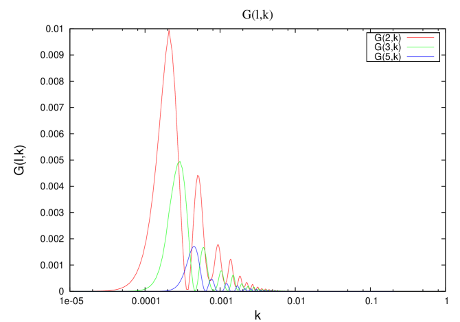
is shown in the Fig (1) (with chosen such that the integral in the definition of can be evaluated to a high enough accuracy). For every given , the radiation transport kernel is a highly oscillatory function of the wavenumber . But for any , it has significant (i.e. non-negligible) values only within a small range of values. The brightness fluctuations roughly go as (where is spherical Bessel function while is the conformal time at the epoch of recombination), thus the minimum value of sets a minimum value of at which the kernel takes up non-negligible values. This procedure tells us that since the radiation transfer function is negligible for , no matter how much power is there in sPPS at very small values, the CMB anisotropies cannot be used to probe the sPPS at these (very large scales). This sets the below which we cannot probe the sPPS. Similarly, given the fact that we have observations only till a maximum value of , this sets the maximum value of up to which we need to sample the kernel: thus, the smallest possible angular resolution of a CMB experiment shall set the lmax that we can probe which shall set a , i.e. sPPS at scales smaller than this scale can not be probed by CMB experiments. Thus, determines while determines . Within this range, one discretizes the space in such a way that the transfer function can be sampled sufficiently well and the above integral can be performed to the desired accuracy. 444 As we shall see in section 4, this number is 6200, thus our matrix shall have dimensions .
Apart from this consideration, the actual observed s are also noisy (due to cosmic variance, instrumental noise and the effect of masking the sky). Thus Eq (1) can be written as a set of linear equations
| (8) |
where is the number of bins in space and is the noise term. Thus the problem we wish to solve is: given the matrix , the few observations (s), the moments of the random variables , how can we find the set of numbers ? In this paper, we shall use the binned CMB data to find sPPS. The number of (binned and hence uncorrelated) data points (WMAP) is (call it ). To sample the kernel satisfactorily, we divide the space into points (). Thus, we have a problem with a set of noisy linear equations and unknowns to be determined.
2.2 Bayesian inversion
Recovering the primordial power spectrum from the observed can be casted as a Bayesian inversion problem in the following way. The posterior probability of obtaining the primordial power spectrum given a kernel and observed is given by:
| (9) |
where is the likelihood and is the prior probability. For our case the denominator (evidence) works just a normalization and we can ignore it.
For the case of Gaussian noise 555 Even though the noise on s is not Gaussian, we proceed pretending the noise to be Gaussian. This is justified because by the central limit theorem: since the chi-squared distribution is the sum of independent random variables with finite mean and variance, it converges to a normal distribution for large . the likelihood function can be written as
| (10) |
where
| (11) |
for the case when the noise covariance matrix is diagonal.
Since for our problem the number of unknowns i.e., are far more than the number of known i.e., therefore ordinary chi square minimization is of no use since it can make the chi square too low 666even if we knew all the parameters, the presence of noise shall ensure that shall be a sum of normalized Gaussians. . In order to avoid chi square taking unphysical values we need some form of regularization in the form of prior. In place of maximizing the likelihood function we maximize the posterior probability.
It has been a common practice to consider the following form of prior for any regularization problem
| (12) |
where is the regularization parameter and is the regularization function. There have been many form of regularization function like quadratic form etc.
In the present work we use an Entropy function as a regularization function which is defined in the following way
| (13) |
where is a parameter which parametrizes the entropy functional we use.
With the regularization function the posterior probability distribution can be written as
| (14) |
where
| (15) |
Maximum entropy method is a particular (nonlinear) inversion method. Here the regularization function is non-quadratic so that the equations to be dealt with to solve the optimization problem shall turn out to be non-linear. Without such a maximum entropy (ME) constraint, the inversion problem is ill-posed (since the data can be satisfied by an infinity of primordial power spectra). The condition that the entropy be a maximum selects one among these. There exist, in the literature, various arguments justifying the use of MEM over other ways of inversion (often using arguments from information theory 777It is often argued that while the maximum likelihood method approach selects the spectrum that has the largest probability of reproducing the data, the maximum entropy method, instead, selects the positive spectrum to which is associated the largest number of ways of reproducing the data, i.e., the one that maximizes the information-theory definition of the entropy of the spectrum subject to the given constraints. ), at this stage, we just treat it as just another nonlinear version of the general regularization scheme.
3 The Cambridge Maximum Entropy Algorithm
So, the problem that we wish to solve involves a highly under-determined system of linear equations. As was mentioned in the last section, one way in which we can attempt to solve this problem is to formulate it as a problem involving the optimization of a non-quadratic function (which will require solving a set of non-linear equations) subject to a constraint. Since the number of unknowns is so large, we have to solve the corresponding constrained non-linear optimization problem in a very large dimensional space. Also, we have other constraints that we need to take care of e.g. the components of are positive quantities (since is a power spectrum), so the optimization algorithm that we use must not cause the components of to become negative (this requirement rules out methods such as the steepest ascent). Similarly, since the the objective function is quite different from a pure quadratic form, methods such as conjugate gradient method are not very useful.
Experience has shown that one of the strategies which work (despite being complicated) is the following: instead of searching for a minimum in a single search direction (e.g. in steepest ascent method), one searches in a small- (typically three-) dimensional subspace. This subspace is spanned by vectors that are calculated at each point in such a way as to avoid directions leading to negative values. The algorithm that we use is based on the one developed by Skilling and Bryan [21, 22] and is sometimes referred to as The Cambridge Maximum Entropy Algorithm. It has been extensively used in not only radio astronomy but also in other fields. Here we quickly review this algorithm for the sake of completeness.
3.1 Entropy and
The problem to be solved involves finding a set of (with maximum entropy) from a data set . For any , let
| (16) |
We shall use the following definition of entropy (the non-linear regularization function)
| (17) |
here, is a fixed number (sometimes called “the default”) that sets the normalization of . Notice that . This gives, (since is fixed),
| (18) |
telling us that and . It is easy to see that entropy surfaces are strictly convex. Also, the expression for the various derivatives of the entropy tell us that the solution is the global maximum of entropy, this fact shall be important later. The measure of misfit that we shall use (in order to use the data) is the Chi-squared function
| (19) |
from which we get, the gradient of
| (20) |
and the Hessian
| (21) |
For a linear experiment, the surfaces of constant chi-squared are convex ellipsoids in N-dimensional space. The largest acceptable value for at 99 percent confidence is about (with being the number of observations), see [21]. As the above equations show, quantities such as gradient of and Hessian of can be easily evaluated (though finding the Hessian of is the one of the most computationally expensive tasks since the matrix is and Hessian of shall be matrix).
At every iteration, instead of searching for the maximum of and minimum of along a line, we search in an dimensional subspace of the parameter space. So, instead of
| (22) |
we shall have (with being search directions)
| (23) |
Sufficiently near any point, every function can be approximated by a quadratic function (provided the higher order terms in the Taylor expansion can be ignored). So, within the subspace we shall model the entropy and chi-squared by
| (24) | |||
| (25) |
where and are quadratic
| (26) | |||
| (27) |
which correspond to the first three terms in the Taylor series expansion of and . The first order term in the Taylor expansion of is
which tells us what should be. Similarly, , and can be found:
| (28) | |||||
| (29) | |||||
| (30) |
Thus, if we know the basis vectors, we can find the quadratic functions and .
Obviously, the above definitions shall not be valid to arbitrary distances from the point in question. The quadratic models are reliable only in the vicinity of the current where cubic and higher powers can be neglected. Thus, the step size at each iteration must be such that
| (31) |
for some . We thus need to define the concept of distance in this abstract space. Recall that this means we need to define a metric
| (32) |
note that the metric is different from the function defined by Eq. (26). Experience (see [21]) has shown that the following definition of distance works well
| (33) |
this needs to be compared with the expression for the Hessian matrix of entropy (notice that ). It is straightforward to show that
| (34) |
while choosing to be of works well (see [21]). The algorithm works in the following way: at every iteration, when we are at a point in the space, one considers a distance region s.t. the quadratic model is a good approximation in that region. We now find a subspace and within this subspace, we try to find the place where
-
1.
is maximum,
-
2.
equals some , and,
-
3.
the distance of this new point from the old point is smaller than .
3.2 Construction of the subspace
So, how do we decide the basis vectors which span the subspace? One of our aims is to find the maximum of entropy on the surface of ellipsoid corresponding to . So, naturally, the direction of gradient of entropy must be one of the basis vectors. Since the metric in the space of interest is not Cartesian, there shall be a distinction between contravariant and covariant components of vectors in the space. Since the “position vector” of any point is , a contravariant vector, gradient such as is going to be a covariant vector. So the first (contravariant) basis vector is
| (35) |
The meaning of this direction is easy to understand by recalling its equivalent in usual Cartesian space. In the usual situation, (i.e. if we are at any point, and we go in the direction by a distance of , the change in the value of the function is ). It is obvious from this expression that when is parallel to the direction of gradient, the change is maximum. Thus, to maximize the change in , we shall move in the direction parallel to so that
| (36) |
This equation should be compared with the definition of the first basis vector, Eq [35] (and since the Kronecker delta is the metric in a Cartesian space, the two equations are equivalent). Thus, the first basis vector tells us the direction in which the entropy change per unit distance is maximum.
Similarly, another basis vector could be
| (37) |
since we wish to change the at every iteration so that we eventually reach the surface. If we find what the two search directions (defined above) become after incrementing by , the direction shall stay within the subspace spanned by and but the direction shall go out of the subspace (see [22]). This suggests that we choose more basis vectors such as
| (38) | |||||
| (39) |
Experience has shown that a family of three or four such search directions gives quite a robust algorithm for solving the problem. In our problem, we chose the third search direction to be
| (40) |
where, the following Eqs define the lengths and which are the gradient vectors
| (41) |
our experience has shown that putting the factors of and in the definition of the third basis vector improves the speed of convergence of the answer.
3.3 Optimization within the subspace
Once we have found the subspace (by finding the basis vectors in the space of all s), we proceed as follows: we now wish to find the step, the coefficients in Eq (23). To do this, we shall solve a corresponding constrained optimization problem in the dimensional subspace (as was stated in the previous subsection, we worked with , but we shall continue to explain the details for a general ). Since the functions and are quadratic, the problem in the subspace is much simpler: it is a simple problem of quadratic programming (quadratic objective function with quadratic constraint). The only additional complication is that the quadratic model is not valid to arbitrary distances from the original point, so we need to satisfy an additional distance constraint.
Let us begin by recalling that both the matrices and are real-symmetric. Also, the matrix is positive definite. The reason is as follows: the way we have defined the metric on the space (see Eq (33) ),
| (42) |
where in the last step we used Eq (34). So, it is clear that is a positive definite matrix (which implies that all its eigenvalues are positive). Thus if one of the eigenvalues of is a small positive number, numerical errors can cause it to become negative. In our implementation of the algorithm, we choose to ignore any directions which are defined by eigenvalues which are too small. Additional simplification occurs if we simultaneously diagonalize the two matrices and . 888 Simultaneous diagonalization Theorem: If and are real symmetric matrices and is positive definite, then there exists an invertible matrix s.t. and is diagonal. The diagonal entries of are the roots of the polynomial . Notice that this is different from finding a basis in which both are diagonal. Here, if is chosen to be identity matrix, then is orthogonal and is the same as . This leads to the unique diagonal representation of the matrix (with the eigenvalues as the diagonal values). Recall that the eigenvalues of a matrix are the solutions of the equation . There exist stable numerical algorithms to achieve this (see e.g. page 463 of [23]) which take in the two real symmetric matrices and and returns the (non-singular) matrix and the diagonal matrix .
After simultaneous diagonalization, within the subspace, the quadratic model functions and are given by
| (43) | |||||
| (44) |
the quantities etc are now defined in terms of the new basis vectors (but the same old definitions). Since this causes the function to become a Kronecker delta, the distance constraint Eq. looks like
| (45) |
We chose the coefficient on the RHS to be and we verified that the actual value of this number is unimportant. Typically, the function is such that all its eigenvalues are (also) positive, then, the minimum value of the function in the subspace (where the above definitions work) is
| (46) |
Thus, no matter what the global aim is, at a given iteration, within the subspace, we can not get to any values below . In fact, even trying to achieve is not a great idea since in that case we shall not use any information about .
The real challenge in the subspace is to satisfy the distance constraint. Many different elaborate tricks have been mentioned in the literature to do this. We choose to not worry about getting a quick answer, hence we do the following: in order to ensure that the distance constraint always gets satisfied (i.e. we do not go too far from the present location in just one step), we shall choose to have a which is not too different from (the present value of ). We thus choose
| (47) |
with chosen to be a small number (e.g. ). This causes the algorithm to take very small “baby steps” towards the answer. Numerical experience has shown that as far as our problem is concerned, this is good enough. Of course, the actual value of or chosen is not important as long as the distance constraint gets satisfied.
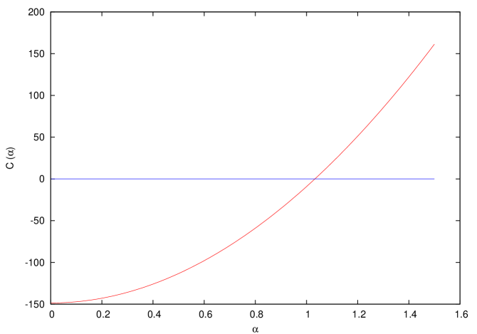
The problem in the sub space is thus simplified to finding the point such that the function is maximum subject to the constraint that (and an additional constraint that the distance constraint must get satisfied). The technique of Lagrange’s undetermined multiplier is useful here: we wish to find the point on the curve where is maximum, to find the desired point, we consider the set of points at which all the partial derivatives of the function
| (48) |
(for an undetermined ) vanish. For any , such points are given by
| (49) |
So, for every value of , find the value of and then the function : we are after that value of which leads to so we look for a solution of the equation . The function is a monotonically increasing function of , see fig. (2). Since the function often happens to be a quickly changing function of (especially while it is changing its sign), the solution for needs to be found to a high tolerance level.
3.4 Stopping criterion
In solving the constrained optimization problem, one fact which becomes important is the following: at the point at which the constrained optimization problem gets solved, the gradient vectors of the two functions become parallel. Thus, if we find the unit vector in the direction of gradient of entropy and in the direction of gradient of chi squared function, the dot product of these two unit vectors (defined using the entropy metric) must become negligible as we head towards the point at which the constrained optimization problem gets solved. The unit vectors in the directions of gradients are (with and defined previously)
| (50) |
We thus expect the angle
| (51) |
to become too small (compared to a unit radian) as the algorithm proceeds (Fig(3)).
4 Recovering Primordial Power Spectrum
In this section, we shall (i) test the formalism presented in the previous section by trying to recover a featureless as well as feature-full sPPS from simulated noisy CMB data and (ii) apply the algorithm to actual WMAP 7 year binned TT angular power spectrum [1] to recover the Primordial Power Spectrum. Thus, to begin with, we shall find out the radiation transfer function for the simplest set of assumptions, inject a featureless sPPS and get noise-free (which we shall refer to as theoretical s). Next we shall add noise to these pure s.
4.1 The radiative transport kernel
First, we need to set the values of the various cosmological parameters and get the corresponding radiation transfer function. This can be done by making use of the codes such as CMBFAST [5], CAMB [6] or gTfast [7]. The results in this section are got from transfer function found using the code gTfast which itself is based on CMBFAST (version 4.0). It is important to notice that since in this work we shall only use the data, so, we only calculate the temperature radiation transfer function. To find out the transport kernel, we assume that the universe is spatially flat and dark energy is a cosmological constant (i.e. we have a spatially flat CDM universe) and set the values of the cosmological parameters to their WMAP nine year values [1] (WMAP9 + bao + h0): the values of various parameters to be fed into the code gTfast are given in table 1. We also assume that there are no tensor perturbations to the metric. We use Peebles recombination (rather than using RECFAST) and assume that the Primordial fluctuations are completely adiabatic. Finally ,we shall not correct the transfer function for lensing of CMB, SZ effect or other effects that cause secondary anisotropies of CMB. This shall give us the radiation transfer function from which we can easily evaluate the matrix . For the case we are dealing with, the matrix shall have dimensions . Finally, we would like to state that the results one obtains and conclusions that one draws should better not depend on the exact values of these parameters.
| Parameter | value |
|---|---|
| lmax | 1500 |
| ketamax | 3000 |
| 0.0472 | |
| 0.2408 | |
| 0.712 | |
| 0.0 | |
| 69.33 km/s/Mpc | |
| Tcmb | 2.72548 K |
| 0.308 | |
| (massless) | 3.04 |
| (massive) | 0.0 |
| 0.088 |
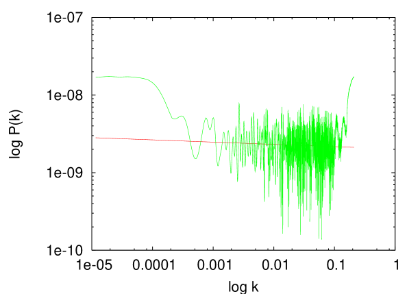
4.2 Recovering test spectra
We can now inject a test sPPS which is a power law with (with and K) and get the corresponding theoretical s, and add noise. The noise we add is dominated by cosmic variance at low (less than 600) values while for high values, the noise is dominated by instrumental errors. Fig (4) shows the result of using the algorithm described in the previous section to recover the sPPS in the present case. The following points are worth noting:
-
1.
To get the result shown in Fig (4), we set the parameter in Eq (17) to be . As was stated, the solution is the location of global maximum of entropy in the space. From
(52) it is clear that corresponds to being . Thus, this value of corresponds to the situation in which is the solution with the maximum value of entropy.
-
2.
In an actual CMB experiment (such as WMAP) the amount of noise (instrumental as well as that due to cosmic variance) is not the same for all scales, which means that our data is not equally good for all values of . Fig (4) shows that at scales at which the noise is large (very low and very high values which will correspond to very low and very high values), the recovered tends to approach the value , the recovery (at these scales) tends to be poor. Thus, at scales at which the noise is too large (or the kernel takes up negligible values), the recovery depends on what is the prior information we have about the solution. Thus the range of values in which we can recover the PPS is too restricted.
-
3.
Even at scales at which the noise is smaller (and at which we hope to recover well), we can have wiggly artificial features in the recovered PPS (in the form of peaks and dips). In the recovered power spectrum there could exist three kinds of features: (i) those which are actually there in the injected PPS (which are not there in the present case), (ii) those which are not there in the PPS but got introduced by the algorithm itself (these shall change as we change ) and finally, (iii) those which are artifacts of the added noise (a particular realization of the noise shall have outliers, if we consider different realizations of the noise, we shall get different recoveries).
-
4.
The scales at which we typically introduce features in the sPPS are roughly MPc-1 to MPc-1. We would like the recovery to be good at these scales. If we have data till very large value of , and the noise at these large values is very low compared to the noise at s corresponding to the above scales, the algorithm shall ignore the few data points with larger noise and try to only take the data at the other scales seriously. Thus, if we wish to recover better at these scales we must focus on recovering the PPS using only the data from the values corresponding to these scales. Thus, having data till larger values of multipole moment with lesser noise may not help.
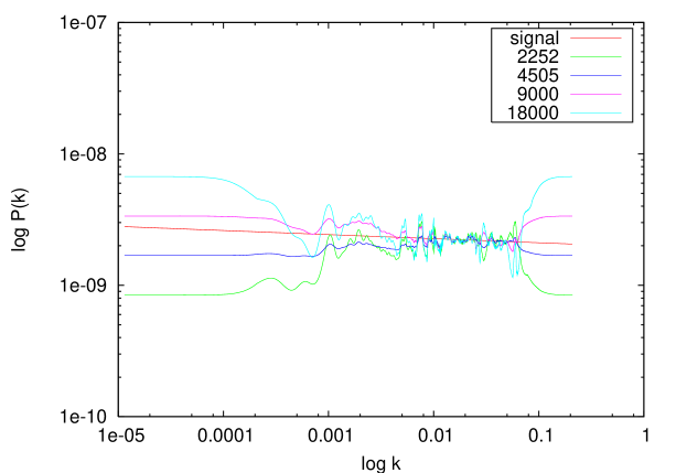
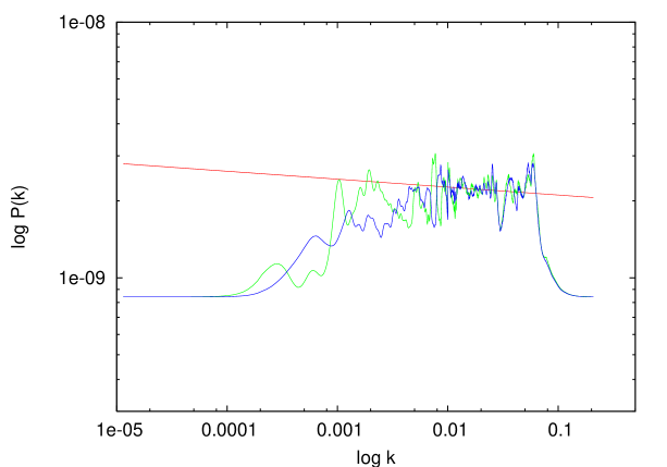
In practise, the process of masking the sky causes the various s to get correlated. The simplest situation in which we can hope to recover the sPPS is the one in which the the data points corresponding to different values are uncorrelated. This happens for the binned CMB data set (which has data only for 45 values). To make use of the binned data, we also work with a binned kernel which is defined
| (53) |
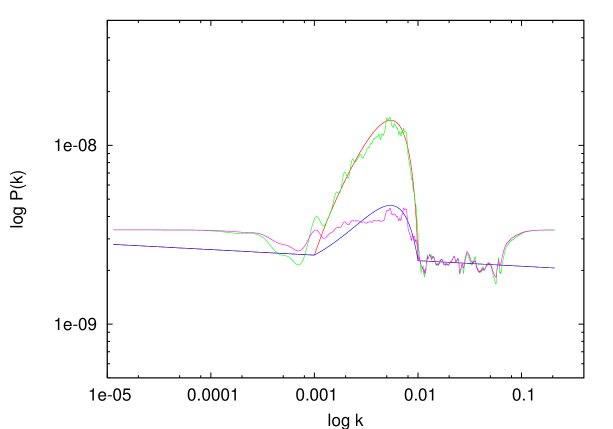
where is the number of values in the bin. By using this averaged kernel and applying the algorithm to simulated binned data (with the added noise equal to the noise for WMAP 7 year binned data), we get the results shown in Fig (5) (this time we show the results for many values). We again get an answer which at scales at which the noise is large, tends to the value of the default (i.e. ) while at scales at which the noise is relatively low, the recovery tends to fluctuate around the featureless injected signal. For a fixed value of , the recovery at scales at which the noise is relatively lower shall be different if we consider different realizations of the noise. This is illustrated in Fig (6): here the recovery shall be the same at scales with no data and shall be different at scales with data. The key question is whether we can recover features in the sPPS by this method. The fact that this can be done is illustrated in Fig (7): we just introduce a bumpy feature between the scales MPc-1 to MPc-1 and vary its height and see that unless the height of the bump is too small, the algorithm can recover it. Of course if we introduce a feature at a scale at which the data is not good or at which the kernel takes up negligible values, the feature shall not be recovered. Moreover, it is not surprising that the recovery is much better if the feature is more prominent.
4.3 WMAP 7 year binned CMB data
In this sub-section we apply the algorithm to actual CMB data. We use WMAP 7 year binned data set and use it to recover the sPPS. The result is shown in fig 8. The details of the recovery of course depend on the chosen value of the parameter . In the present context, the value of represents our a priori knowledge (without using any data) of how much we think should be the scalar fluctuation in the metric in the early universe.

It may appear that if the conclusion depends on such an a priori knowledge, we may not get anything worthwhile. But the following fact is worth noting: it is seen that at scales at which the noise is lesser, even though the recovered depends on the value of chosen, this dependence is quite weak and quite predictable (as we increase a lot or decrease it a lot, the recovery just “stretches” in the direction in the plane). An interesting exercise is this: if, without using the CMB data, we still knew that the amplitude of the scalar metric perturbations is (roughly) , then what can this method of deconvolution tell us about the sPPS? Fig (10) illustrates how the red tilt of the PPS can be detected in such a case. One can keep on decreasing the value of and see what happens. In this context, the case of is very interesting since this corresponds to using another familiar definition of entropy, the recovery for this case is illustrated in Fig (10). What is interesting is that if we choose to be too small, we begin to get an IR cut-off not very different from the one reported in the literature previously (see [17]), but, we also get an apparent UV cut-off. Moreover, such a small value of causes the artificial features to get stretched so much that we may not consider the reconstruction to be trustworthy in this case.
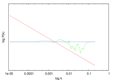
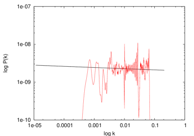 Figure 10: Choosing causes the features to get overly “stretched ”and we find apparent IR and UV cut-offs in power.
5 Summary and discussion
In this work, we attempted to probe the amplitude and shape of scalar primordial power spectrum (sPPS) using the CMB data. We fixed the values of various cosmological parameters (apart from the ones specifying the sPPS itself) and formulated the problem as an inverse problem. To solve the inverse problem, we use the maximum entropy method which is a non linear regularization method. There exist many possible ways to employ the maximum entropy regularization, we use a particular definition of entropy and a particular algorithm to solve the corresponding constrained non-linear optimization problem in a very large dimensional parameter space.
The way we have formulated the problem, there exists a parameter (which we called ) whose value decides the location of global maximum of entropy in the space of all s. In the absence of any data, the algorithm shall just send every initial guess to the global maximum of entropy. Even in the presence of data, the following is worth noting
-
1.
at scales where
-
(a)
we have noisy data (so, little or no information), or,
-
(b)
the kernel (to be inverted) takes up negligible values (again too large or too small values),
the recovered by MEM depends on the value of chosen (as is the ME solution), while at the scales where the data is good, we recover something which has comparatively lesser dependence on what we choose.
-
(a)
-
2.
at scales at which the data is good, the recovered by MEM is consistent with a power law primordial power spectrum (with any possibly small deviations which we can not say anything about at this stage). This can be seen by comparing fig (8) with figs (5) and (7). While the existence of any small deviations from power law behaviour can not be completely ruled out, this analysis reinforces our belief that any such possible deviations must be small.
This is by no means the last word on the existence of features in sPPS, this is not even the last word on the use of MEM for this purpose.The implementation of our algorithm to this problem till now does not seem to give any reason to believe that there are any serious deviations from the power law. We would like to mention that this is not completely unexpected, even in the light of existing papers such as [17] because the error bars at scales at which the features were recovered in those works are very large: the maximum entropy method can not claim any features at scales where the error bars are so large 999This “rules out” (or at least renders them untrustworthy) many models of inflation considered in the literature in recent times.. This analysis shows that at scales at which the CMB data is trustworthy, the Primordial Power Spectrum of scalar metric perturbations is, to a very good approximation, a power law.
In future, one can look at the following prospects. We should be able to solve this problem of possible existence of features in sPPS without assuming the values of other cosmological parameters (i.e. without formulating this problem as a simple inversion problem). Even in the present formulation, there may be ways of combining results from different values of to get a better recovery. One may wish to use the actual WMAP likelihood (or rather, the corresponding ) as a measure of misfit, but this is not easy in the way we have attempted to solve the problem (we need to know the and its first two derivatives). Also, we have lost a lot of information in the process of binning the kernel and working with the binned, uncorrelated data. We would like to use all that lost information. Similarly, we have only used the angular power spectrum of CMB, we would also like to use the polarization spectra to probe the sPPS. We may also need to post-process the recovered sPPS to get more useful information. Another interesting possibility worth exploring is the connection of Maximum Entropy deconvolution with other ways of deconvolution (e.g. Richard Lucy deconvolution).
Appendix A Testing the method
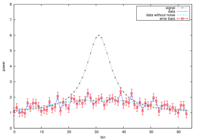
The main text described the material necessary to employ the maximum entropy inversion in any circumstance. The following points need to be noted (these are just tried and tested facts about the algorithm, many of which are illustrated here for the case of a toy problem shown in Fig(11), whose solution is given in Fig (12)):
-
•
If we did not have any data available, the optimization problem would have involved maximizing entropy subject to no constraints. In such a scenario, the solution we should get must be as that is where the global maximum of entropy is.
-
•
If the value of is such that the of the global maximum of entropy is smaller than , then is itself the desired solution since “the data are too noisy for any information to be extracted” (see the last paragraph of page 113 of [21]).
-
•
It is not a surprise at all that choosing too small value of should lead to negative value for entropy (the fact that depending upon the choice of , sometimes we could be at locations in the parameter space with negative value of has no impact on the solution of the problem), see Fig (13).
-
•
In Eq (48), corresponds to the unconstrained maximization of irrespective of . If we are too close to the global maximum of entropy (), the value of required to solve the constrained optimization problem in the subspace (for defined by Eq (48)) shall become too large. In this situation, it may be difficult to numerically find any solution for .
-
•
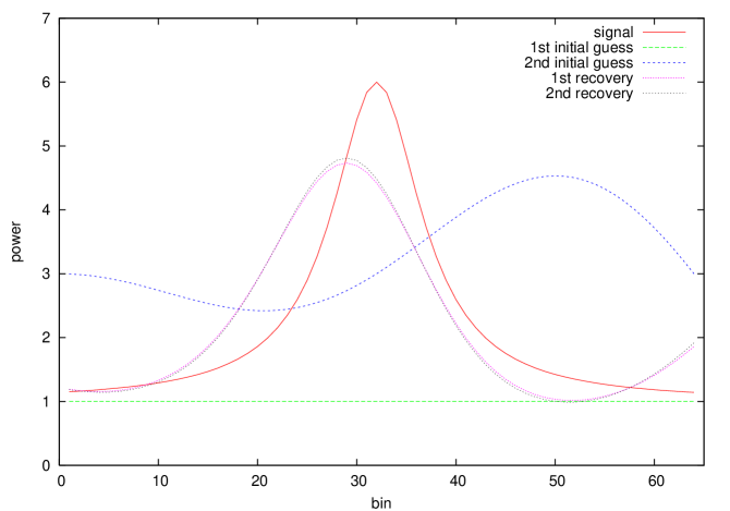
As long as we do not stay too close to the global maximum of entropy (so that numerical problems such as those stated in the previous point above do not turn up), the choice of the initial guess for running the algorithm is immaterial. That is, all the initial guesses shall lead to the same answer (see Fig (12)).
-
•
All the above problems can be easily avoided if we just choose a value of s.t. the of configuration is much higher than the of initial guess (which better be more than ). Notice that this is not a requirement, just a trick. Also, this does not help us in finding any unique preferable value of .
-
•
For many kernels the exact value of chosen does not matter as far as the recovered is concerned, as long as the final value of becomes sufficiently small compared to a unit radian, all recoveries with different final are almost the same. The of signal (for a given realization) shall just fluctuate around (roughly) , we have tested that if is set equal to , the recovery does not change. This happens to be true e.g. for the case of CMB kernel, the case of our interest.
-
•
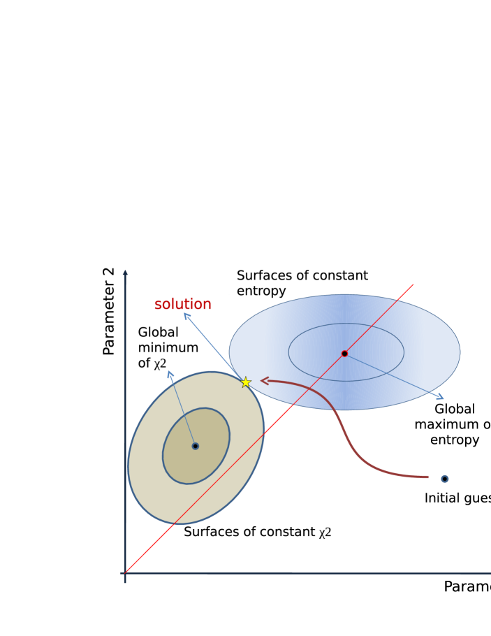
The exact details of the shape of the final recovered solution does depend upon the actual value of chosen: the surface can be thought of as a closed ellipsoidal surface in the dimensional -space while as we change , we define the line as being the location of global maximum of entropy for these different values of . This will of course mean that as we change , the place where the entropy is maximum on the surface shall also change. Thus, as we continuously change , we shall get a family of recoveries (see fig (13)). So, the details of the recovered answer depends on the chosen value of this free (or adjustable) parameter. But since the global maximum of entropy is at , the value of represents the “background” (i.e.a priori) knowledge of how much the power in various bins is, without using any knowledge of data at all.
-
•
Whether the recovery is good or bad, depends on the details of the kernel. For the case of CMB kernel, we have tested that the recovery is often quite good.
Acknowledgment: The authors acknowledge the use of WMAP data and the use of codes such as CMBFAST, gTfast and CAMB. The authors would also like to thank Tarun Souradeep (IUCAA, Pune) for reading through the manuscript and giving useful comments. GG thanks Rajaram Nityananda (NCRA, Pune), Mihir Arjunwadkar (CMS, Pune university, Pune), Abhilash Mishra (CALTECH, Pasadena) and Ranjeev Misra (IUCAA, Pune) for discussions at various stages of the work. GG thanks Council of Scientific and Industrial Research (CSIR), India, for the research grant award No. 10-2(5)/2006(ii)-EU II. JP acknowledge support from the Swarnajayanti Fellowship, DST, India (awarded to Prof. Tarun Souradeep, IUCAA, Pune, India).
References
- [1] E. Komatsu et al. 2011 ApJS 192 18 (arXiv:1001.4538); arXiv: 1212.5226;
- [2] A.A. Starobinsky, Phys. Lett. B 91, 99 (1980); D. Kazanas, Ap. J. 241, L59 (1980); A. H. Guth, Phys. Rev. D 23, 347 (1981); A. D. Linde, Phys. Lett. B108, 389 (1982); A. Albrecht and P. J. Steinhardt, Phys. Rev. Lett. 48, 1220 (1982).
- [3] A.A. Starobinsky, JETP Lett. 30, 682 (1979); Mukhanov V. F., Chibisov G. V., 1981, ZhETF Pis ma Redaktsiiu, 33, 549; Hawking S. W., 1982, Physics Letters B, 115, 295; A.A. Starobinsky, Phys. Lett. B 117, 175 (1982); Guth A. H., Pi S.Y., 1982, Physical Review Letters, 49, 1110.
- [4] A. Linde, arXiv: hep-th/ 0503203; D. H. Lyth and A. R. Liddle, The Primordial Density Perturbation, Cambridge University Press, 2009; D. Baumann, arXiv:astro-ph/0907.5424v1; D. Langlois, arXiv:astro-ph/1001.5259v1; L. Sriramkumar, arXiv:astro-ph/0904.4584v1.
- [5] U. Seljak and M. Zladarriaga, Astrophys. J. 469, 437 (1996).
- [6] A. Lewis, A. Challinor and A. Lasenby, Astrophys. J. 538, 473 (2000), (http://camb.info/).
- [7] Komatsu and Spergel, PRD 63, 063002 (2001);
- [8] Antony Lewis and Sarah Bridle Phys. Rev. D 66, 103511 (2002).
- [9] Jayanti Prasad and Tarun Souradeep Phys. Rev. D 85, 123008 (2012); Kiyotomo Ichiki1 and Ryo Nagata Phys. Rev. D 80, 083002 (2009); Kiyotomo Ichiki1, Ryo Nagata1, and Jun’ichi Yokoyama1 Phys. Rev. D 81, 083010 (2010);
- [10] Dhiraj Kumar Hazra et al JCAP10(2010)008; Dhiraj Kumar Hazra et al 1106.2798v2;
- [11] Rajeev Kumar Jain, Pravabati Chingangbam, Jinn-Ouk Gong, L. Sriramkumar, Tarun Souradeep, JCAP 09 01: 009, 2009 [arXiv:astro-ph/0809.3915].
- [12] Rajeev Kumar Jain, Pravabati Chingangbam, L. Sriramkumar, Tarun Souradeep Phy. Rev. D 82 023509 (2010) [arXiv:astro-ph/0904.2518].
- [13] Ryo Saito, Jun’ichi Yokoyama, Ryo Nagata JCAP06(2008)024; Rajeev Kumar Jain, Pravabati Chingangbam, L. Sriramkumar JCAP 07 10: 003, 2007. [arXiv:astro-ph/0703762]; Sirichai Chongchitnan, George Efstathiou JCAP 07 01: 011, 2007.
- [14] Edgar Bugaev, Peter Klimai Phys. Rev. D 78, 063515 (2008).
- [15] Samuel M. Leach and Andrew R. Liddle Phys. Rev. D 63, 043508 (2001) [arXiv:astro-ph/0010082].
- [16] A. A. Starobinsky Pis’ma Zh. Éksp. Teor. Fiz. 55, 477 (1992) [JETP Lett. 55, 489 (1992)].
- [17] A. Shafieloo and T. Souradeep Phy. Rev. D 70, 043523 (2004); R. Sinha and T. Souradeep Phy. Rev. D 74, 043518 (2006); A. Shafieloo, T. Souradeep, P. Manimaran, P.K. Panigrahi and R. Rangarajan Phy. Rev. D 75, 123502 (2007); A. Shafieloo and T. Souradeep Phy. Rev. D 78, 023511 (2008); Gavin Nicholson and Carlo R. Contaldi JCAP07 (2009) 011; Tocchini-Valentini, D., Hoffman, Y. and Silk, J. MNRAS, 367: 1095-1102, 2006.
- [18] J. Hamann, A. Shafieloo and T. Souradeep JCAP 10 04: 010,2010.
- [19] S. Dodelson, Modern Cosmology (Academic Press, San Diego, U.S.A., 2003).
- [20] Press, William H.; Teukolsky, Saul A.; Vetterling, William T.; Flannery, Brian P., Numerical recipes in FORTRAN. The art of scientific computing Cambridge: University Press, 1992, 2nd ed.
- [21] J. Skilling and R.K. Bryan Mon. Not. R. Astr. Soc. (1984) 211, 111 - 124.
- [22] Skilling, J., and Gull, S.F. 1985, inMaximum-Entropy and Bayesian Methods in Inverse Problems, C.R. Smith and W.T. Grandy, Jr., eds. (Dordrecht: Reidel). Skilling, J. 1986, in Maximum Entropy and Bayesian Methods in Applied Statistics, J.H. Justice, ed. (Cambridge: Cambridge University Press). Gull, S.F. 1989, in Maximum Entropy and Bayesian Methods, J. Skilling, ed. (Boston: Kluwer).
- [23] Matrix Computations (Third Edition) by Gene H.Golub and Charles F.Van Loan