Topological properties of sets represented by an inequality involving distances

Abstract.

Consider a set represented by an inequality. An interesting phenomenon which occurs in various settings in mathematics is that the interior of this set is the subset where strict inequality holds, the boundary is the subset where equality holds, and the closure of the set is the closure of its interior. This paper discusses this phenomenon assuming the set is a Voronoi cell induced by given sites (subsets), a geometric object which appears in many fields of science and technology and has diverse applications. Simple counterexamples show that the discussed phenomenon does not hold in general, but it is established in a wide class of cases. More precisely, the setting is a (possibly infinite dimensional) uniformly convex normed space with arbitrary positively separated sites. An important ingredient in the proof is a strong version of the triangle inequality due to Clarkson (1936), an interesting inequality which has been almost totally forgotten.

1. Introduction

1.1. Background:

Consider a set represented by an inequality. An intuitive rule of thumb says that its interior is the set where strict inequality holds, its boundary is the set where equality holds, and the closure of the interior is the closure of the set itself. This intuition probably comes from familiar and simple examples in $\mathbb{R}^{n}$ such as balls, halfspaces, and polyhedral sets, or the ones described in [15, p. 192],[25, p. 6]. Another well known example is the case of level sets of convex functions. Given a convex function $f:\mathbb{R}^{n}\to\mathbb{R}$, denote its so-called 0-level set by

$$S:=f^{\leq 0}:=\{x\in\mathbb{R}^{n}:f(x)\leq 0\}.$$ (1)

If the so-called Slater’s condition holds [5, p. 325],[6, p. 44], [45], [47, p. 98], namely that $f(x_{0})<0$ for some $x_{0}\in\mathbb{R}^{n}$, then the interior of $S$ is $f^{<0}:=\{x\in\mathbb{R}^{n}:f(x)<0\}$. See, for instance, [42, p. 59]. This property can be easily generalized to any topological vector space when $f$ is assumed to be continuous [47, pp. 80, 117]. An additional closely related well-known result says that the closure of a convex set $C$ whose (relative) interior is nonempty is the (relative) closure of the (relative) interior of the set [6, pp. 8-9],[23, p. 114],[42, p. 46] ($\mathbb{R}^{n}$), [47, pp. 29-30] (topological vector space). This property can be expressed as $\overline{C}=f^{\leq 1}=\overline{f^{<1}}$, where $f(x)=p(x-x_{0})$, $x_{0}\in\textnormal{int}(C)$ is given, and $p$ is the Minkowski functional (the gauge) associated with $C-x_{0}$ (this is a consequence of [47, Theorem 2.21, Remark 2.22(a), p. 27] and [47, Theorem 2.27, p. 29]).

Yet another example, which is related to the second one mentioned above, is the case of star bodies. These objects are important ones in the geometry of numbers theory [7, 13, 20, 28, 29, 32, 33]. A set $K\subseteq\mathbb{R}^{n}$ is called a star body whenever there exists a function $f:\mathbb{R}^{n}\to\mathbb{R}$, called a distance function, such that $K=f^{\leq 1}$ and $f$ has the following properties: it is continuous, nonnegative, does not coincide with the zero function, and finally, for all $t\geq 0$ and $x=(x_{k})_{k=1}^{n}\in\mathbb{R}^{n}$ the equality $f(tx)=tf(x)$ holds. (Sometimes one can find slightly different formulations of the definition of star bodies, such as in [28] where it is assumed that $f(tx)=|t|f(x)$ for all $t\in\mathbb{R}$ and $x\in\mathbb{R}^{n}$. However, in common scenarios all of these formulations are essentially equivalent.) Typical examples of distance functions which illustrate the richness of this class of functions are

$$f(x)=C\left(\prod_{k=1}^{n}|x_{k}|^{p_{k}}\right)^{1/\sum_{k=1}^{n}p_{k}}\quad\textnormal{and}\quad f(x)=\left|\sum_{k=1}^{r}C_{k}|x_{k}|^{p}-\sum_{k=r+1}^{n}C_{k}|x_{k}|^{p}\right|^{1/p}$$

and multiplications, additions or subtractions of such functions (with suitable powers and absolute values). Here $C,p,p_{1},\ldots,p_{n}$ are given positive numbers, $C_{1},\ldots,C_{k}$ are non-negative numbers such at least one of them is positive, and $r$ is a given integer in $[1,n]$ (and $\sum_{k=r+1}^{n}p_{k}:=0$ when $r=n$). If, as in [44], only distance functions obtained from norms are considered, then the corresponding star body is bounded. However, in general it may not be bounded as in the case where the distance function is $f:\mathbb{R}^{2}\to\mathbb{R}$ defined by $f(x_{1},x_{2})=|x_{1}^{2}-x_{2}^{2}|^{1/2}$.

The subset $f^{=1}$ is called the boundary of $K$ and the subset $f^{<1}$ is called the interior of $K$. These subsets play an important role in the theory of the geometry of numbers in the context of evaluating the number of lattice points of certain lattices (critical lattices) in certain regions. It turns out that they coincide with their topological colleagues, and moreover, $f^{\leq 1}=\overline{f^{<1}}$. See, e.g., [7, pp. 105-107] for the simple proof of this claim and related ones. These properties can be generalized to star bodies contained in topological vector spaces.

1.2. The phenomenon discussed in this paper:

This paper discusses a phenomenon similar to the one described above, where now the set $S$ has the form of a Voronoi cell (or a dominance region) of a given site $P$ with respect to another given site $A$, namely

$$S=\{x\in X:d(x,P)\leq d(x,A)\}=:\textnormal{dom}(P,A).$$ (2)

The sites $P$ and $A$ are nothing but nonempty subsets contained in a convex subset $X$ which is contained in a normed space, $d(x,P)=\inf\{d(x,p):p\in P\}$, and $d$ is the distance function induced by the norm. The sites are assumed to be positively separated, that is,

$$d(P,A):=\inf\{d(p,a):p\in P,a\in A\}>0.$$ (3)

The set $S$ (which is nonempty since $P\subseteq S)$ can be represented in the form (1) where $f:X\to\mathbb{R}$ is defined by $f(x)=d(x,P)-d(x,A)$ for all $x\in X$, but in general this function is not convex and hence one cannot conclude in advance that the above mentioned phenomenon holds for it (see also the paragraph after the next one).

The Voronoi cell is the basic component in what is known as the Voronoi diagram, a geometric structure which appears in many fields in mathematics, science, and technology and has diverse applications [3, 10, 8, 14, 17, 20, 34]. Given a tuple of nonempty sets $(P_{k})_{k\in K}$ called the sites or the generators, the Voronoi cell (or Voronoi region) of the site $P_{k}$ is the set of all points in the space whose distance to $P_{k}$ is not greater than their distance to the other sites $P_{j},j\neq k$. In other words, the Voronoi cell of $P_{k}$ is nothing but the dominance region $R_{k}=\textnormal{dom}(P_{k},A_{k})$ where $A_{k}=\cup_{j\neq k}P_{j}$. The Voronoi diagram is the tuple of Voronoi cells $(R_{k})_{k\in K}$. See Figures 4-4 for a few illustrations. Voronoi diagrams have been the subject of an investigation for more than 160 years, starting formally with Dirichlet [12] and Voronoi [48] in the context of the geometry of numbers and informally with Descartes (astronomy) or even before. They have been considerably investigated during the last 40 years, but mainly in the case of point sites in finite dimensional Euclidean spaces (frequently only in $\mathbb{R}^{2}$ or $\mathbb{R}^{3}$). Not much is known about them in other settings, e.g., in the case of non-Euclidean norms or sites having a general form (but some works studying them there do exist: see, e.g., the discussion below, the discussion in Example 4.2, and some references mentioned in [39]). Papers studying them in an infinite dimensional setting seem to be rare at the moment [24, 37, 38].

The main result of this paper is Theorem 3.3 which establishes that under the above mentioned assumptions on the sites, if the normed space belongs to the wide class of uniformly convex spaces (see Section 2), then

$$\partial(\textnormal{dom}(P,A))=\{x\in X:d(x,P)=d(x,A)\},$$ (4)

$$\textnormal{int}(\textnormal{dom}(P,A))=\{x\in X:d(x,P)<d(x,A)\},$$ (5)

$$\textnormal{dom}(P,A)=\overline{\{x\in X:d(x,P)<d(x,A)\}},$$ (6)

where $\partial(S)$, $\textnormal{int}(S)$, and $\overline{S}$ are respectively the boundary, interior, and closure of the set $S$ (with respect to $X$). The property expressed in (4)-(6) may seem intuitively clear at first glance, and even true in any metric space, but simple counterexamples show that this is not the case even in $\mathbb{R}^{2}$ (see Example  4.2, Figure  4, and Remark  3.2). The set $\{x\in X:d(x,P)=d(x,A)\}$ is called the bisector of $P$ and $A$, and the property expressed in (4) implies that a bisector of two positively separated sites in a uniformly convex space cannot be “fat”, that is, it cannot contain a ball (see Figure 4 for a counterexample).

In the case of finite dimensional uniformly convex spaces (i.e., finite dimensional strictly convex spaces) (4)-(6) are essentially known, at least in the 2-dimensional case with certain sites (e.g., points or polygonal sets), but it seems that only recently these properties have been established, in a closely related formulation, in the case of general dimension and general closed sites [22, Lemma 6]. A somewhat related discussion [21] in the case of point sites in a finite dimensional real strictly convex normed space implies that the induced bisector is homeomorphic to a hyperplane. When the space is not strictly convex, then (4) does not necessarily hold as is known for a long time, since the bisectors can be fat or strange: See the discussion in Example 4.2. In this connection it is interesting to note that it is known for a long time that the convexity of the Voronoi cell of two point sites $P$ and $A$ (or the fact that the bisectors are hyperplanes) characterizes the Euclidean norm [11, 18, 19, 30, 49]. This can be generalized to the case of Voronoi cells induced by lattices [18, 19, 30]. See also [31] regarding related properties of bisectors induced by two point sites in finite dimensional normed spaces.

Another result related to (4)-(6) is [24, Lemma 5.1, Lemma 5.2]. The setting now is any (possibly infinite dimensional) uniformly convex space. In its simple version the result says that $\textnormal{dom}(P,A)$ is homeomorphic to a closed and bounded convex set whenever $P=\{p\}$ where $p$ is a point contained in the (relative) interior of $X$ and whenever $X$ is closed and bounded. This generalizes the well-known fact that in the Euclidean norm the Voronoi cell of a point site is convex. One cannot expect to generalize the above in a naive way to the case where $P$ is general, since now $\textnormal{dom}(P,A)$ is not necessarily connected (see Figure 4).

1.3. Issues related to the proof:

The main difficulty in trying to establish (4)-(6) in the general case of infinite dimensional spaces and general sites $P$ and $A$ is the fact that the distance between a point and a set is not necessarily attained even if the set is closed. The reason why this property is so helpful is because it gives one candidates for satisfying some desired conditions, candidates which are absent in the general case. The idea is to look for the candidates along a certain interval, somewhat similarly to the case of proving that the closure of a the (nonempty) interior of a convex set is the closure of the set itself (Subsection 1.1). More specifically, if $z\in X$ is on the bisector of $P$ and $A$, i.e., it satisfies the equation $d(z,P)=d(z,A)$, then because of (4) one needs to show in particular that in every neighborhood of $z$ there are points outside $\textnormal{dom}(P,A)$, i.e., points $x\in X$ satisfying $d(x,A)<d(x,P)$. If $d(z,A)$ is attained at some point $a\in A$, then one may guess that the needed points $x$ can be taken from the segment $[a,z)$ near the endpoint $z$. It turns out that this is indeed true because of the uniform (actually strict) convexity of the space as shown in [22, Lemma 6] and this is true even if $d(P,A)>0$ is weakened to $P\cap A=\emptyset$. Unfortunately, as mentioned above, in infinite dimensional spaces the distance between a point and a general set is not necessarily attained.

The way the above mentioned difficulty is treated here is by using the assumption that $d(P,A)$ is positive and by using a nice and interesting improvement of the triangle inequality, due to Clarkson [9, Theorem 3]. This strong triangle inequality (as called in [9]) allows one, after a suitable selection of certain parameters, to derive explicit geometric estimates which show that if the above mentioned point $z$ is in the interior of $\textnormal{dom}(P,A)$, then a contradiction must occur. Interestingly, although the strong triangle inequality was formulated in the very famous paper [9] of Clarkson, it has been almost totally forgotten (in contrast to the well-known Clarkson’s inequalities for $L_{p}$ spaces [9, Theorem 2]). Actually, in spite of a comprehensive search the author has made, evidences to its existence were found only in [9] and later in [35, 46]. It will not be surprising if additional references will be found, but it seems that this strong triangle inequality is far from being a mainstream knowledge. Recently this inequality has been used for proving another property of Voronoi cells, namely their geometric stability with respect to small changes of the sites [38] (see also Subsection 1.4). The derivation of [24, Lemma 5.1, Lemma 5.2] mentioned above is based indirectly on the strong triangle inequality via some of the results established in [38].

1.4. Possible applications:

It may be of some interest to mention a few possible applications of the main result. One application is related to the geometric stability of Voronoi cells with respect to small changes of the sites. As shown in [38], a small perturbation of the sites, measured using the Hausdorff distance, yields a small perturbation in the Voronoi cells, measured again using the Hausdorff distance. In several applications related to Voronoi diagrams, such as in robotics [43], the bisectors of the cells are important. Hence one may ask whether the bisectors are geometric stable under small perturbations of the sites. It turns out that (4) enables one to deduce this, assuming no neutral Voronoi region exists, i.e., the union of the Voronoi cells is the whole space (this always holds when finitely many sites are considered and also holds in many scenarios involving infinitely many sites, such as the case of lattices; however, in general a neutral region can exist). The proof is essentially as the proof of [39, Corollary 5.2] (despite the somewhat different setting). This issue will be discussed in a revised version of [38] which is is planned to be uploaded onto the arXiv soon.

Another application of the main result is as an auxiliary tool in the proof that a certain iterative scheme involving sets converges to certain geometric objects. These objects are variations of the concept of Voronoi diagram and formally they are defined as the solution of a fixed point equation on a product space of sets. The pioneering work of Asano, Matoušek, and Tokuyama [2] (earlier announcements appeared in [1]) introduced and discussed an important member in this interesting family of objects. This object, called “a zone diagram”, was studied in [2] in the case of the Euclidean plane with finitely many point sites. An iterative scheme for approximating it was suggested there.

Soon after [2], in an attempt to better understand zone diagrams, the concept of “a double zone diagram” was introduced and studied in [41] in a general setting ($m$-spaces: a setting which is more general than metric spaces). However, no way to approximate this object was suggested. Recently [40] it has been shown that the algorithm suggested by Asano, Matoušek, and Tokuyama converges in a rather general setting (a class of geodesic metric spaces which contains Euclidean spheres and finite dimensional uniformly convex spaces and infinitely many sites of a general form) to a double zone diagram, and sometimes also to a zone diagram. An important part in the proof was to establish (6) in the above mentioned setting. A careful inspection of the whole proof shows that in order to generalize the convergence to infinite dimensional uniformly convex normed spaces it is sufficient to prove (6) there and to make some modifications in certain additional auxiliary tools. This issue, which is a work in progress, will be discussed elsewhere.

1.5. Paper layout:

The paper is laid as follows. In Section 2 the concept of uniformly convex normed spaces is recalled and the strong triangle inequality of Clarkson is presented. The main result is established in Section 3. In Section 4 a few examples and counterexamples related to the main result are discussed. Section 5 concludes the paper.

2. Uniformly convex spaces and the strong triangle inequality

This section recalls the concept of uniformly convex normed spaces and presents the strong triangle inequality of Clarkson.

Definition 2.1.

A normed space $(\widetilde{X},|\cdot|)$ is said to be uniformly convex if for each $\epsilon\in(0,2]$ there exists $\delta\in(0,1]$ such that for all $x,y\in\widetilde{X}$ satisfying $|x|=|y|=1$, if $|x-y|\geq\epsilon$, then $|(x+y)/2|\leq 1-\delta$.

Typical examples of uniformly convex spaces are inner product spaces, the sequence spaces $\ell_{p}$, the Lebesgue spaces $L_{p}(\Omega)$ ($1<p<\infty$), and a uniformly convex product of finitely many uniformly convex spaces. The spaces $\ell_{1},\ell_{\infty},L_{1}(\Omega),L_{\infty}(\Omega)$ are typical examples of spaces which are not uniformly convex. See [4, 9, 16, 27, 36] for more information.

From the definition of uniformly convex spaces it is possible to obtain a function which assigns to the given $\epsilon$ a corresponding value $\delta(\epsilon)$. There are several ways to obtain such a function, but for the purposes of this paper $\delta$ should be increasing and to satisfy $\delta(0)=0$ and $\delta(\epsilon)>0$ for all $\epsilon\in(0,2]$. A familiar choice, which is not necessarily the most convenient one, is the modulus of convexity

$${\delta(\epsilon)=\inf\{1-|(x+y)/2|:|x-y|\geq\epsilon,\,|x|=|y|=1\}}.$$

For formulating the strong triangle inequality the definition of Clarkson’s angle should be recalled.

Definition 2.2.

Given two non-zero vectors $x,y$ in a normed space, the angle (or Clarkson’s angle, or the normed angle) $\alpha(x,y)$ between them is the distance between their directions, i.e., it is defined by

$$\alpha(x,y)=\left|\frac{x}{|x|}-\frac{y}{|y|}\right|.$$

Theorem 2.3.

(Clarkson [9, Theorem 3]) Let $x_{1},x_{2}$ be two non-zero vectors in a uniformly convex normed space $(\widetilde{X},|\cdot|)$. If $x_{1}+x_{2}\neq 0$, then

$$|x_{1}+x_{2}|\leq|x_{1}|+|x_{2}|-2\delta(\alpha_{1})|x_{1}|-2\delta(\alpha_{2})|x_{2}|,$$ (7)

where $\alpha_{l}=\alpha(x_{l},x_{1}+x_{2}),\,l=1,2$.

The original formulation of Clarkson’s theorem is for finitely many non-zero terms (whose sum is not zero too) in a uniformly convex Banach space. An examination of the (simple) proof shows that the theorem actually holds in any normed space, not necessarily uniformly convex or Banach. However, it seems less useful in general normed spaces where it may happen that $\delta(\epsilon)=0$ even when $\epsilon>0$. Inequality (7) can obviously be extended to the case of zero terms by letting $\alpha(0,x):=0=:\alpha(x,0)$ for all $x$, but no use of this extension will be made here.

3. The main result

In this section the main result (namely Theorem 3.3 below) is proved. The proof is also based on a simple lemma which is proved for the sake of completeness. Before stating both, here are a few words about the (standard) notation used below: $B(x,r)$ denotes the open ball with radius $r>0$ and center at $x\in X$; given points $a,b\in X$, the segments $[a,b]$ and $[a,b)$ denote the sets $\{a+t(b-a):t\in[0,1]\}$ and $\{a+t(b-a):t\in[0,1)\}$ respectively; given a subset $S$ of $X$, its complement, closure, interior, boundary, and exterior (with respect to $X$) are respectively $S^{c}$,$\overline{S},\textnormal{int}(S),\partial(S)$ and $\textnormal{Ext}(S):=(\overline{S})^{c}$; given a norm $|\cdot|$, the induced metric is $d(x,y)=|x-y|$. Given $f:X\to\mathbb{R}$, recall that $f^{\leq 0}=\{x\in X:f(x)\leq 0\}$ and $f^{=0}=\{x\in X:f(x)=0\}$. Similarly $f^{<0}$, $f^{\geq 0}$, and $f^{>0}$ are defined.

Lemma 3.1.

Let $(X,\tau)$ be a topological space let $f:X\to\mathbb{R}$. If $f^{\leq 0}$ is closed and $f^{<0}$ is open, then:

1. $f^{<0}\subseteq\textnormal{int}(f^{\leq 0})$;

2. $f^{>0}=\textnormal{Ext}(f^{\leq 0})$;

3. $\partial(f^{\leq 0})\subseteq f^{=0}$;

4. equality holds in (a) if and only it holds in (c);

5. if $\textnormal{int}(f^{\geq 0})=f^{>0}$, then $f^{\leq 0}=\overline{f^{<0}}$;

In particular, the above items hold when $f$ is continuous.

Proof.

1. Since $f^{<0}$ is open by assumption and it is contained in $f^{\leq 0}$, the assertion follows from the fact that $\textnormal{int}(f^{\leq 0})$ is the union of all the open subsets of $f^{\leq 0}$.

2. $\textnormal{Ext}(f^{\leq 0}):=\left(\overline{f^{\leq 0}}\right)^{c}=\left(f^{\leq 0}\right)^{c}=f^{>0}$ by definition and because $f^{\leq 0}$ is assumed to be closed.

3. Suppose that $x\in\partial(f^{\leq 0})$. Then $x$ cannot belong to $f^{<0}$ which is contained in $\textnormal{int}(f^{\leq 0})$ by part (a), and cannot belong to $f^{>0}=\textnormal{Ext}(f^{\leq 0})$ by part (b). Thus $x\in f^{=0}$.

4. Follows from $\partial(f^{\leq 0})\bigcup\textnormal{int}(f^{\leq 0})=\overline{f^{\leq 0}}=f^{\leq 0}=f^{=0}\bigcup f^{<0}$ and the fact that the terms in both unions are disjoint.

5. Follows from $f^{<0}=(f^{\geq 0})^{c}$ and $(\textnormal{int}(S))^{c}=\overline{S^{c}}$ for each $S\subseteq X$.

∎

Remark 3.2.

Neither the equality $f^{\leq 0}=\overline{f^{<0}}$ nor the equality $\partial(f^{\leq 0})=f^{=0}$ imply each other. A simple counterexample to the first case is obtained from the function $f:\mathbb{R}\to\mathbb{R}$ defined by $f(x)=-|x|$ if $|x|\leq 1$ and $f(x)=|x|-2$ when $|x|\geq 1$. The problem is with $x=0$. A counterexample to the second case is $g=-f$.

Theorem 3.3.

Let $X$ be a convex subset of a uniformly convex normed space $(\widetilde{X},|\cdot|)$. Let $P,A\subseteq X$ be nonempty and suppose that $d(P,A)>0$. Then (4), (5), and (6) hold.

Proof.

It is possible to write $\textnormal{dom}(P,A)=f^{\leq 0}$ where $f:X\to\mathbb{R}$ is the continuous function defined by $f(x)=d(x,P)-d(x,A)$ for each $x\in X$. It suffices to show that (4) holds. Indeed, (5) will be a obtained as a consequence of Lemma 3.1(d). But then, by noticing that obviously $d(A,P)>0$, it will be possible to obtain (4) and (5) with the roles of $P$ and $A$ exchanged, i.e., with $g=-f$ instead of $f$. This and Lemma  3.1(e) (still applied to $f(x)=d(x,P)-d(x,A)$) will imply (6).

It will now be shown that (4) holds. The inclusion $\partial(\textnormal{dom}(P,A))\subseteq\{x\in X:d(x,P)=d(x,A)\}$ is implied by Lemma 3.1(c). For the converse one, let $z$ be in the set $\{x\in X:d(x,P)=d(x,A)\}$. Assume by way of contradiction that $z\notin\partial(\textnormal{dom}(P,A))$. It must be that $d(z,P)>0$, because otherwise $d(z,A)=d(z,P)=0$ and hence $d(P,A)=0$, a contradiction. Since $z\in\textnormal{dom}(P,A)\backslash\partial\textnormal{dom}(P,A)$ it follows that $z\in\textnormal{int}(\textnormal{dom}(P,A))$. Thus there exists $\epsilon\in(0,d(z,P))$ such that the ball $B(z,\epsilon)$ is contained in $\textnormal{dom}(P,A)$. Let $\sigma\in(0,\infty)$ be arbitrary and let

$$r=\displaystyle{\min\left\{\sigma,\frac{d(P,A)}{4},\frac{\epsilon}{2}\cdot\delta\left(\frac{d(P,A)}{4(\sigma+d(z,A))}\right)\right\}}.$$ (8)

For $r$ to be well defined the argument inside $\delta$ should be at most 2 (see page 2). This is true without any assumption on $\sigma$. Indeed, given $\tau>0$ arbitrary, let $a^{\prime}\in A$ and $p^{\prime}\in P$ satisfy $d(z,a^{\prime})<d(z,A)+\tau$ and $d(z,p^{\prime})<d(z,P)+\tau$. The triangle inequality and the equality $d(z,P)=d(z,A)$ imply that $d(P,A)\leq d(p^{\prime},a^{\prime})\leq 2d(z,A)+2\tau$, and since $\tau$ was arbitrary this implies that $d(P,A)/(4(d(z,A)+\sigma))<0.5<2$.

Now let $a\in A$ and $p\in P$ satisfy

$$d(z,a)<r+d(z,A)\quad\text{and}\quad d(z,p)<d(z,P)+r/10.$$ (9)

From the choice of $a,p,z$, and $\epsilon$,

$$\epsilon<d(z,P)\leq d(z,a)<r+d(z,A)=r+d(z,P)\leq r+d(z,p).$$ (10)

By (10) the length of the segment $[a,z]$ is greater than $\epsilon$. Let $x\in[a,z]\subset X$ be such that $d(x,z)=\epsilon/2$. Then $x\in B(z,\epsilon)\subseteq\textnormal{dom}(P,A)$ and hence $d(x,P)\leq d(x,a)$. Let $q\in P$ satisfy $d(x,q)\leq d(x,P)+r/10$. By the above

$$d(x,q)\leq d(x,P)+r/10\leq d(x,a)+r/10.$$ (11)

By the choice of $p$ and $\epsilon$

$$d(x,z)=\epsilon/2<\epsilon<d(z,p)\leq d(z,P)+r/10\leq d(z,q)+r/10.$$ (12)

This and the fact that $\epsilon-r/10>\epsilon/2$ imply that $q\neq x$ and $q\neq z$. In addition, because of (11), $x\in[a,z]$, (9), and (8) it follows that

$$d(q,z)\leq d(q,x)+d(x,z)\leq d(a,x)+d(x,z)+r/10\\ =d(z,a)+r/10<d(z,A)+\sigma+r/10.$$ (13)

For arriving at the desired contradiction distinguish between two cases.

Case 1: The angle $\alpha(z-x,z-q)$ satisfies the inequality

$$\alpha(z-x,z-q)\geq d(P,A)/(4(\sigma+d(z,A))).$$ (14)

In this case by (9), the strong triangle inequality (7), by (11), by $2d(z,x)=\epsilon$, by (14), by the monotonicity of $\delta$, by $x\in[a,z]$, by (8), and by (10) it follows that

$$d(z,p)\leq d(z,P)+r/10\leq|z-q|+r/10\\ \leq r/10+|z-x|+|x-q|-2|z-x|\delta(\alpha(z-x,z-q))-2|x-q|\delta(\alpha(x-q,z-q))\\ \leq r/10+|z-x|+|x-a|+r/10-\epsilon\delta(d(P,A)/(4(\sigma+d(z,A))))\\ \leq|z-a|+r/5-2r\leq d(z,p)+r-9r/5<d(z,p),$$

a contradiction. All the angles are well defined because $z\neq x$, $z\neq q$ and $q\neq x$.

Case 2: Inequality (14) does not hold. Let $\theta=(q-z)/|q-z|$ and $\phi=(x-z)/|x-z|$. Then $q=z+|q-z|\theta$. Since $x\in[a,z]$ it follows that $a=z+|a-z|\phi$ and

$$|\phi-\theta|=|(-\phi)-(-\theta)|=\alpha(z-x,z-q).$$ (15)

Let $s=d(z,a)-d(z,q)$. By (13) it follows that $s\geq-r/10$. By (10), (9), and $q\in P$

$$d(z,a)-r<d(z,p)\leq d(z,P)+r/10\leq d(z,q)+r/10.$$ (16)

This and (8) imply that $s<11r/10\leq 11d(P,A)/40$. By combining this with $s\geq-r/10$ we see that $|s|\leq 11d(P,A)/40$. By this inequality, the definition of $s$, by (13), by (15), since (14) does not hold, and since $r/10<\sigma+d(z,A)$,

$$|a-q|=\left|(z+|a-z|\phi)-(z+|q-z|\theta)|=|(s+|q-z|)\phi-(|q-z|\theta)\right|\\ \leq|s||\phi|+|q-z||\theta-\phi|<\frac{11d(P,A)}{40}+\frac{(d(z,A)+\sigma+r/10)d(P,A)}{4(\sigma+d(z,A))}\\ \leq d(P,A)(11/40+1/2)<d(P,A),$$

a contradiction because $q\in P$ and $a\in A$. This contradiction and the previous established one show that the assumption $z\not\in\partial(\textnormal{dom}(P,A))$ is false and prove (4) (and (5)-(6)). ∎

4. Examples and Counterexamples

This section presents a few examples and counterexamples related to Theorem  3.3.

Example 4.1.

Illustrations of Theorem 3.3 are given in Figures 4 and 4. In both figures the Voronoi diagrams of several sites $(P_{k})_{k\in K}$ are presented and the corresponding dominance regions are the Voronoi cells $\textnormal{dom}(P_{k},A_{k})$, $A_{k}=\bigcup_{j\neq k}P_{j}$. In Figure 4 the setting is a square in $(\mathbb{R}^{2},\ell_{2})$ and each site is a point, and in Figure 4 the setting is a square in $(\mathbb{R}^{2},\ell_{p}),\,p\approx 2.71$ and each site has two points.

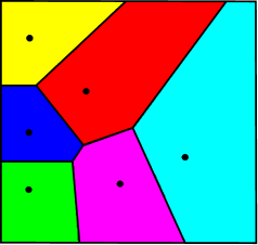
Figure 1. The Figure of Example  4.1 (Euclidean norm).

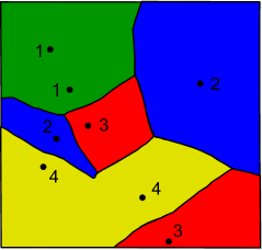
Figure 2. The figure of Example  4.1 (the $\ell_{p}$ norm, $p\approx 2.71$).

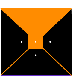
Figure 3. The setting of Example  4.2. The shown shape is the Voronoi cell of $P=\{(0,0)\}$ with respect to $A=\{(-2,0),(2,0),(0,-2)\}$, in a square in $(\mathbb{R}^{2},\ell_{\infty})$.

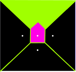
Figure 4. The setting of Figure 4 and Example 4.2. The set of strict inequality is the small purple “house” (pentagon) in the middle. The set of equality (the full green “W”, the sides of the house, and the rays) contains a large part of the interior.

Example 4.2.

When the space is not uniformly convex, then the conclusion of Theorem  3.3 does not necessarily hold. Indeed, consider $\textnormal{dom}(P,A)$ where $P=\{(0,0)\}$ and $A=\{(-2,0),(2,0),(0,-2)\}$, in the square $[-5,5]^{2}$ in $(\mathbb{R}^{2},\ell_{\infty})$. See Figure 4. The set of strict inequality is relatively small (the “house” around $P$) compared to the set where equality holds (the bisector). This latter set contains a large part of the interior. See Figure 4. In fact, when $X=\mathbb{R}^{2}$, then the former set remains the same (and hence bounded) while the latter grows and it is not bounded. A closely related example is [21, Example 4]. The setting there is the lattice of point sites generated by the vectors $(2,0),(0,8)$ in $(\mathbb{R}^{2},\ell_{\infty})$ and the considered cell is of the site $P=\{(0,0)\}$. In this case $A$ is the set of all other sites. The resulting Voronoi cell is bounded and it is the union of a small middle hexagon (strict inequality) and large concave pentagons (bisector). The difference between the example of Figure  4 (which was discovered before the author become aware to [21, Example 4]) and [21, Example 4] is that in [21, Example 4] no rays appear as in the case of Figure 4. Additional related examples can be found in [3, p. 390, Figure 37] ($P=\{(-1,1)\}$, $A=\{(1,-1)\}$ in $(\mathbb{R}^{2},\ell_{1})$) and [26, p. 605, Fig. 1(b)], [34, p. 191, Figure 3.7.2] ($P=\{(-1,-1)\}$, $A=\{(1,1)\}$ in $(\mathbb{R}^{2},\ell_{1})$) where, for instance, the bisector in the first case is $\left((-\infty,-1]\times[1,\infty)\right)\cup\{(t,-t):t\in[-1,1]\}\cup\left([1,\infty)\times(-\infty,-1]\right)$. Now the set of strict inequality is not bounded.

Example 4.3.

This example shows that the condition $d(P,A)>0$ in Theorem 3.3 cannot be weakened to $P\cap A=\emptyset$ without further assumptions. Indeed, let $(\widetilde{X},|\cdot|)$ be the infinite dimensional Hilbert space $\ell_{2}$. Let $X=\widetilde{X}$ and

$$P=\{e_{1}\}\cup\{((n+1)/n)e_{n}:n=2,3,4,\ldots\},\quad A=\{((n+2)/n)e_{n}:n=2,3,4,\ldots\},$$

where $e_{n}$ is the $n$-th element in the standard basis, i.e., its $n$-th component is 1, and the other components are 0. For $z=0$ the equality $1=d(z,e_{1})=d(z,P)=d(z,A)$ holds. However, $z$ is in the interior of $\textnormal{dom}(P,A)$ since a simple check shows that the ball $B(z,0.1)$ is contained in $\textnormal{dom}(P,A)$. Thus (4) does not hold.

Example 4.4.

This example shows that if $P\cap A\neq\emptyset$, then Theorem 3.3 may be violated even in the case of a 2-dimensional space (in contrast to the case where $P\cap A=\emptyset$ as mentioned in Subsection 1.2). Indeed, let $(\widetilde{X},|\cdot|)$ be $\mathbb{R}^{2}$ with the Euclidean norm and let $X=\mathbb{R}^{2}$. Let $P=\{(-10,0),(0,0)\}$ and $A=\{(0,0),(10,0)\}$. Let $S=[-1,1]\times\mathbb{R}$. Then $S\subset[-2,2]\times\mathbb{R}\subseteq\textnormal{dom}(P,A)$. Thus $S\subset\textnormal{int}(\textnormal{dom}(P,A))$. But $d(z,P)=d(z,A)=d(z,(0,0))$ for each $z\in S$. Therefore (4) does not hold.

5. Concluding remarks

It may be of interest to further investigate the phenomenon described in this note in various domains of mathematics and to find interesting applications of it. Perhaps a discontinuous version related to the phenomenon can be formulated (a simple example where this holds: let $C=f^{\leq 0}$ where $f:\mathbb{R}^{n}\to\mathbb{R}$ is defined as $0$ on the boundary of the unit ball, arbitrarily positive outside the ball and arbitrarily negative inside the ball). This may help in the study of singularities of the boundary.

Another possible direction for future investigation is to weaken the assumption of uniform convexity to strict convexity (the unit sphere does not contain line segments but, in contrast to uniform convexity, now there is no uniform bound $\delta(\epsilon)>0$ on how much the midpoint $(x+y)/2$ should penetrate the unit ball assuming $|x|=|y|=1$ and $|x-y|\geq\epsilon$). We conjecture that in this case there are counterexamples to Theorem  3.3. Alternatively, one may try to work with general normed spaces (under additional assumptions on the sites) or with spaces which are not linear. As a matter of fact, recently [39, 40] certain related results have been obtained. In the first paper (See Section 7 in the current arXiv version) a closely related result (Lemma 9.11) is used as a tool for proving the geometric stability of Voronoi cells with respect to small changes of the sites in normed spaces which are not uniformly convex, under some assumptions on the relation between the structure of the unit sphere and the configuration of the sites. In the second paper (see Section 7) again a closely related result is used for proving the convergence of an iterative scheme for computing a certain geometric object in a class of geodesic metric spaces. However, in both cases the distance between any point in the space and both sites $P$ and $A$ is assumed to be attained and hence the case of arbitrary sites in an infinite dimensional setting is not in the scope of these results.

Finally, studying sets represented by a system of inequalities instead of one inequality may be valuable, because, for instance, sets having this form appear frequently in optimization [5, 6, 42]. In the case of Voronoi cells $R_{k}=\textnormal{dom}(P_{k},\cup_{j\neq k}P_{j})$ one observes that the cell is nothing but the sets of all points $x$ satisfying the system of inequalities $f_{j}(x)\leq 0$ where $f_{j}(x)=d(x,P_{k})-d(x,P_{j})$ for all $j\in K,j\neq k$. A simple check shows that $d(x,\cup_{j\neq k}P_{j})=\inf\{d(x,P_{j}):j\neq k\}$ and hence, when $K$ is finite, one concludes from Theorem 3.3 that $x\in\partial R_{k}$ if and only if $x$ satisfies the above system of inequalities and at least one inequality is equality, and $x\in\textnormal{int}(R_{k})$ if and only if $x$ satisfies the system of inequalities with strict inequalities.

References

- [1] T. Asano, J. Matoušek, and T. Tokuyama, The distance trisector curve, Adv. Math. 212 (2007), 338–360, a preliminary version in STOC 2006, pp. 336–343.
- [2] by same author, Zone diagrams: Existence, uniqueness, and algorithmic challenge, SIAM J. Comput. 37 (2007), 1182–1198, a preliminary version in SODA 2007, pp. 756-765.
- [3] F. Aurenhammer, Voronoi diagrams - a survey of a fundamental geometric data structure, ACM Computing Surveys 3 (1991), 345–405.
- [4] Y. Benyamini and Y. Lindenstrauss, Geometric nonlinear functional analysis. Vol. 1, American Mathematical Society Colloquium Publications, vol. 48, American Mathematical Society, Providence, RI, 2000.
- [5] D. P. Bertsekas, Nonlinear programming, second ed., Athena Scientific, Belmont, Mass., 1999.
- [6] J. M. Borwein and A. L. Lewis, Convex analysis and nonlinear optimization: Theory and examples, second ed., CMS books in Mathematics, Springer, USA, 2006.
- [7] J. W. C. Cassels, An Introduction to the Geometry of Numbers, Classics in mathematics, Springer, Berlin-New York, 1997 (reprint of the 1971 edition).
- [8] S. N. Chiu, D. Stoyan, W. S. Kendall, and J. Mecke, Stochastic geometry and its applications, third ed., Wiley, 2013.
- [9] J. A. Clarkson, Uniformly convex spaces, Trans. Amer. Math. Soc. 40 (1936), 396–414.
- [10] J. H. Conway and N. J. A. Sloane, Sphere Packings, Lattices, and Groups, third ed., Springer-Verlag, New York, 1999.
- [11] M. M. Day, Some characterization of inner-product spaces, Trans. Amer. Math. Soc. 62 (1947), 320–337.
- [12] L. Dirichlet, Über die reduction der positiven quadratischen Formen mit drei unbestimmten ganzen zahlen, J. Reine. Angew. Math. 40 (1850), 209–227.
- [13] M. M. Dodson and S. Kristensen, Khintchine’s theorem and transference principle for star bodies, Int. J. Number Theory 2 (2006), 431–453.
- [14] Q. Du, V. Faber, and M. Gunzburger, Centroidal Voronoi tessellations: applications and algorithms, SIAM Rev. 41 (1999), no. 4, 637–676.
- [15] W. Fulks, Advanced calculus: an introduction to analysis, John Wiley and Sons, New York, 1961.
- [16] K. Goebel and S. Reich, Uniform convexity, hyperbolic geometry, and nonexpansive mappings, Monographs and Textbooks in Pure and Applied Mathematics, vol. 83, Marcel Dekker Inc., New York, 1984.
- [17] C. Gold, The Voronoi Web Site, 2008, http://www.voronoi.com/wiki/index.php?title=Main˙Page.
- [18] P. M. Gruber, Kennzeichnende eigenschaften von euklidischen räumen und ellipsoiden I, J. reine angew. Math. 256 (1974), 61–83.
- [19] by same author, Kennzeichnende eigenschaften von euklidischen räumen und ellipsoiden II, J. reine angew. Math. 256 (1974), 123–142.
- [20] P. M. Gruber and C. G. Lekkerkerker, Geometry of Numbers, second ed., North Holland, 1987.
- [21] A. G. Horváth, On the bisectors of a Minkowski normed space, Acta Math. Hungar. 89 (2000), 417–424.
- [22] K. Imai, A. Kawamura, J. Matoušek, D. Reem, and T. Tokuyama, Distance k-sectors exist, Computational Geometry: Theory and Applications 43 (2010), 713–720, preliminary versions in SoCG 2010, pp. 210-215, arXiv 0912.4164 (2009).
- [23] P. J. Kelly and M. L. Weiss, Geometry and convexity, A study in Mathematical methods, John Wiley and Sons, New York, 1979.
- [24] E. Kopecká, D. Reem, and S. Reich, Zone diagrams in compact subsets of uniformly convex spaces, Israel Journal of Mathematics 188 (2012), 1–23, preliminary versions in arXiv:1002.3583 [math.FA] (2010) and CCCG 2010, pp. 17-20.
- [25] T. Lawson, Topology: a geometric approach, Oxford graduate text in Mathematics, Oxford University press, New York, 2003.
- [26] D. T. Lee, Two-dimensional Voronoi diagrams in the Lp-metric, J. ACM 27 (1980), 604–618.
- [27] J. Lindenstrauss and L. Tzafriri, Classical Banach spaces, II: Function spaces, Springer, Berlin, 1979.
- [28] K. Mahler, On lattice points in -dimensional star bodies I. Existence theorems, Proc. Roy. Soc. Lond. A 187 (1946), 151–187.
- [29] by same author, On lattice points in -dimensional star bodies II. (Reducibility theorems), Proc. Kon. Ned. Akad. Wet. 49 (1946), 331–343, 444–454, 524–532, 622–631.
- [30] H. Mann, Untersuchungen über wabenzellen bei allgemeiner Minkowskischer metrik, Monatsh. Math. Phys. 42 (1935), 417–424.
- [31] H. Martini and K.J. Swanepoel, The geometry of Minkowski spaces - a survey. Part II, Expositiones Mathematicae 22 (2004), no. 2, 93–144.
- [32] H. Minkowski, Gesammelte Abhandlungen / von Hermann Minkowski ; unter Mitwirkung von Andreas Speiser und Hermann Weyl ; hrsg. von David Hilbert., New York : Chelsea, 1967, Reprint. Originally published: Leipzig : B.G. Teubner, 1911.
- [33] L. J. Mordell, On the geometry of numbers in some non-convex regions, Proc. London Math. Soc. 48 (1945), 339–390.
- [34] A. Okabe, B. Boots, K. Sugihara, and S. N. Chiu, Spatial Tessellations: Concepts and Applications of Voronoi Diagrams, second ed., Wiley Series in Probability and Statistics, John Wiley & Sons Ltd., Chichester, 2000, with a foreword by D. G. Kendall.
- [35] A. T. Plant, The differentiability of nonlinear semigroups in uniformly convex spaces, Israel J. Math. 38 (1981), no. 3, 257–268.
- [36] S. Prus, Geometrical background of metric fixed point theory, Handbook of Fixed Point Theory (W. A. Kirk and B. Sims, eds.), Kluwer Acad. Publ., Dordrecht, 2001, pp. 93–132.
- [37] D. Reem, An algorithm for computing Voronoi diagrams of general generators in general normed spaces, Proceedings of the sixth International Symposium on Voronoi Diagrams in Science and Engineering (ISVD 2009), pp. 144–152.
- [38] by same author, The geometric stability of Voronoi diagrams with respect to small changes of the sites, (2011), Complete version in arXiv:1103.4125 [cs.CG] (2011), Extended abstract in SoCG 2011, pp. 254-263.
- [39] by same author, The geometric stability of Voronoi diagrams in normed spaces which are not uniformly convex, arXiv:1212.1094 [cs.CG] (2012), (v2; last updated: April 29, 2013).
- [40] by same author, On the computation of zone and double zone diagrams, arXiv:1208.3124 [cs.CG] (2012), (v3; last updated: April 29, 2013).
- [41] D. Reem and S. Reich, Zone and double zone diagrams in abstract spaces, Colloquium Mathematicum 115 (2009), 129–145, arXiv:0708.2668 (2007).
- [42] R. T. Rockafellar, Convex Analysis, Princeton University Press, Princeton, NJ, 1970.
- [43] J. T. Schwartz and M. Sharir, Motion planning and related geometric algorithms in robotics, Proceedings of the International Congress of Mathematicians 1986 (Berkeley, California, USA), vol. 2, American Mathematical Society, 1987, pp. 1594–1611.
- [44] C. L. Siegel, Lectures on the geometry of numbers, Springer-Verlag, Berlin, 1989.
- [45] M. Slater, Lagrange multipliers revisited: a contribution to non-linear programming, Cowles Commission Discussion Paper (Yale University), Mathematics, 403, 1950.
- [46] M. A. Smith and B. Turett, Some examples concerning normal and uniform normal structure in Banach spaces, J. Austral. Math. Soc. (Series A) 48 (1990), 223–234.
- [47] J. van Tiel, Convex Analysis: An Introductory Text, John Wiley and Sons, Chicester:; New York, 1984.
- [48] G. Voronoi, Nouvelles applications des parametres continus à la theorie des formes quadratiques., J. reine. angew. Math. 134 (1908), 198–287.
- [49] A. C. Woods, A characteristic property of ellipsoids, Duke Math. J. 36 (1969), 1–6.