A proposal to implement a quantum delayed choice experiment assisted by a cavity QED

Abstract

We propose a scheme feasible with current technology to implement a quantum delayed-choice experiment in the realm of cavity QED. Our scheme uses two-level atoms interacting on and off resonantly with a single mode of a high Q cavity. At the end of the protocol, the state of the cavity returns to its ground state, allowing new sequential operations. The particle and wave behavior, which are verified in a single experimental setup, are postselected after the atomic states are selectively detected.

Introduction. Recently, the quantum version of Wheeler’s delayed-choice experiment (QDCE) was proposed Terno and experimentally demonstrated for photons Tang2012 ; Popescu ; Kaiser as well as for spins Auccaise ; Mahesh . Different from the classical version Wheeler , which also has been tested in a number of papers DSE , in the QDCE the detecting device can also occupy a quantum state. In general, the goal of delayed-choice experiment is to test the complementarity principle, which states that the wave-like (WL) behavior revealed by the appearance of interference patterns and particle-like (PL) behavior are complementary and mutually exclusive, thus needing two distinct experimental arrangements to be verified. However, the quantum version of QDCE enables one to measure complementary phenomena with a single experimental setup by postselecting the WL or PL behavior, thus pointing to a redefinition of the complementarity principle, such that, instead of complementarity of experimental setups according to Bohr’s view, we have complementarity of experimental data Terno .

Another interesting feature of the QDCE is to prove that there are no consistent local hidden-variable (LHV) theories having “particle” and “wave” as realistic properties. To this prove, the operational definition for “wave” or “particle” was given as the “ability” or “inability” to produce interference Terno . This operational definition was considered further by Filgueiras et al. Filgueiras to show incompatibility between quantum and LHV theories even when arbitrary amounts of white noise is included into the optical QDCE. In this paper, we propose a simplified scheme to realize the analog of the QDCE also in the domain of cavity QED. Our scheme uses only two-level atoms interacting on and off resonantly with a single mode of a cavity, which is disregarded after the interaction, and selective atomic state detectors. The whole setup we are proposing are well known from experiments on cavity QED haroche , thus being completely feasible using current technology.

In the Mach-Zehnder interferometer, as shown in Fig. 1(a), interference patterns giving rise to WL behavior appear in detectors placed on paths $1$ and $0$ when the interferometer is closed, i.e., when the second beam splitter $\mathcal{BS}_{2}$ is present. Otherwise, if the second beam splitter is absent the experiment reveals which-path information, and a PL behavior is observed. In the language of the complementarity principle, if we want to observe the wave aspect of the photon, we must consider the closed interferometer (with $\mathcal{BS}_{2}$ present), whereas to observe the particle nature of the photon we must consider the open interferometer (removing $\mathcal{BS}_{2}$). Note, therefore, that these two different experimental arrangements are complementary in the sense that each choice determines beforehand the statistics of the results by the experimenter’s decision. This is a classical experiment, in the sense that the interferometer has only two states, open or closed.

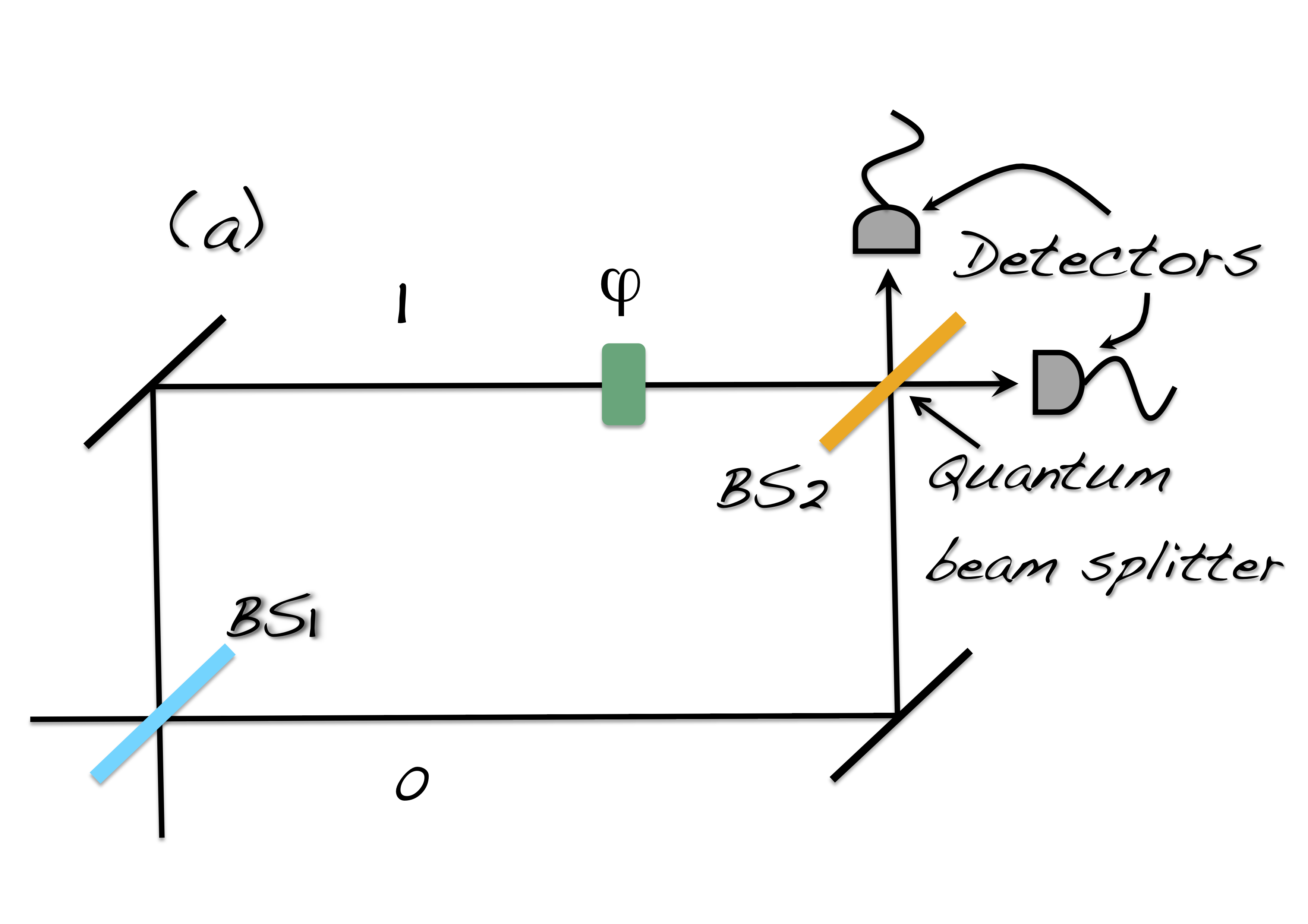
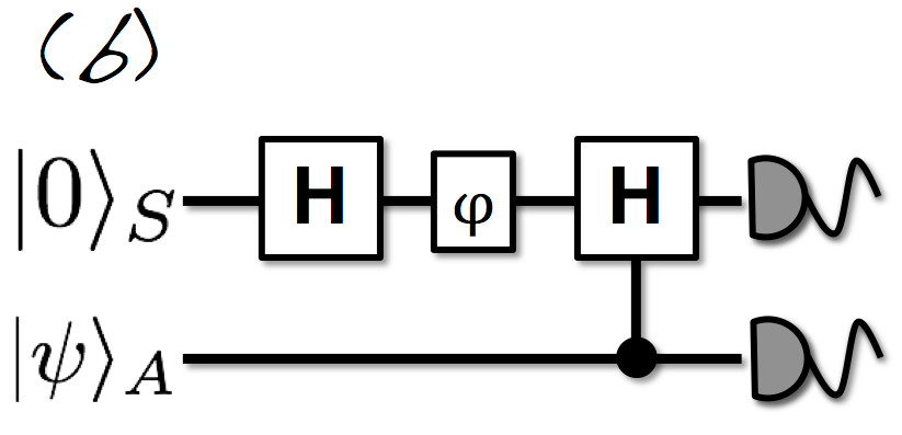
Figure 1: (Color online) (a) Schematic diagram of the Mach-Zehnder interferometer with a quantum beam splitter $BS_{2}$. (b) The quantum circuit that describes the evolution of the ancilla and the photon in the interferometer Terno . The ancilla is the qubit in the lower line of the circuit, while the qubit inside the interferometer is in the upper line. The state of the ancilla is given by $|\psi\rangle_{A}=\cos\alpha|0\rangle_{A}+\sin\alpha|1\rangle_{A}$. $H$ is the Hadamard gate and $\varphi$ is a gate that creates the phase difference $\varphi$ between the paths $0$ and $1$. The interferometer is closed for $\alpha=\pi/2$ and open for $\alpha=0$. For any other value, $0<\alpha<\pi/2$, the interferometer is in a coherent superposition of being closed and open.

In the quantum extension of the delayed choice experiment Terno , the second beam splitter $\mathcal{BS}_{2}$ in Fig. 1(a) is in a coherent superposition of being present and absent and is now controlled by a quantum device, referred to as the ancilla system, which allows the beam splitter to be in a superposition of being present and absent. Fig. 1(b) shows the quantum circuit to describe the evolution of the system through the interferometer. Considering as the initial state of the system- ancilla

$$|\psi\rangle_{\mathcal{SA}}^{in}=|0\rangle_{\mathcal{S}}\otimes\left[\cos\alpha|0\rangle_{\mathcal{A}}+\sin\alpha|1\rangle_{\mathcal{A}}\right]\text{,}$$ (1)

then, after the action of the second beam splitter the final system-ancilla state is

$$|\psi\rangle_{\mathcal{SA}}^{out}=\cos\alpha|p\rangle_{\mathcal{S}}|0\rangle_{\mathcal{A}}+\sin\alpha|w\rangle_{\mathcal{S}}|1\rangle_{\mathcal{A}}\text{,}$$ (2)

where $|p\rangle_{\mathcal{S}}=\left(|0\rangle_{\mathcal{S}}+e^{i\varphi}|1\rangle_{\mathcal{S}}\right)/\sqrt{2}$ accounts for PL statistical behavior of the photon, while $|w\rangle_{\mathcal{S}}=e^{i\varphi/2}\left(\cos\left(\varphi/2\right)|0\rangle_{\mathcal{S}}-i\sin\left(\varphi/2\right)|1\rangle_{\mathcal{S}}\right)$ accounts for its WL behavior, and states $|1\rangle_{\mathcal{S}}$ and $|0\rangle_{\mathcal{S}}$ label the interferometric paths $1$ and $0$, respectively. Note that the transformation employed by the second beam splitter is coherently controlled by the ancillary system, i.e., the ancilla in the state $|0\rangle_{\mathcal{A}}$ corresponds to the absence of the second beam splitter, modeling an open interferometer. On the other hand, the ancilla in the state $|1\rangle_{\mathcal{A}}$ corresponds to $\mathcal{BS}_{2}$ present, then modeling a closed interferometer. Since $\mathcal{BS}_{2}$ is now a quantum system, its state is not limited to be present or absent, but can be in any superposition of $|0\rangle_{\mathcal{A}}$ and $|1\rangle_{\mathcal{A}}$, meaning that the interferometer can be cast in an arbitrary superposition of being open and closed Terno . An interesting behavior displaying a continuous morphing between PL and WL behavior is verified by varying the parameter $\alpha$.

If we now use the computational basis $\left(00,01,10,11\right)$ in the ${\mathcal{S}\otimes\mathcal{A}}$ space, it is straightforward to calculate this final joint probability distribution

$$P\left(S,A\right) = \left[\frac{1}{2}\cos^{2}\alpha,\sin^{2}\alpha\cos^{2}\frac{\varphi}{2},\right.$$ (3)

$$\left.\frac{1}{2}\cos^{2}\alpha,\sin^{2}\alpha\sin^{2}\frac{\varphi}{2}\right]\text{,}$$

with $S$ $\in$ $\mathcal{S}$ and $A$ $\in$ $\mathcal{A}$ representing the measurement outcomes in the computational basis. As demonstrated in Ref.Terno ; Filgueiras , there is no LHV theory that reproduces this set of probabilities, even in the presence of an arbitrary amount of noise.

Controlled interactions. To perform the QDCE assisted by a high$-Q$ cavities we will need the following operators: 

$$H_{on}=\hbar g\left(\sigma^{-}a^{\dagger}+\sigma^{+}a\right)\text{,}$$ (4)

$$H_{off}=\frac{\hbar g^{2}}{\delta}a^{\dagger}a\sigma_{ee}\text{,}$$ (5)

$$R=\hbar(\lambda\sigma^{+}+\lambda^{\ast}\sigma^{-})\text{.}$$ (6)

Eq.(4) is the usual Jaynes-Cummings model scully and describes a resonant atom-field interaction. Here $a^{\dagger}$ and $a$ stands for creation and annihilation operators, respectively, the two-level atom is described by the lowering ($\sigma^{-}$) and raising ($\sigma^{+}$) Pauli operators, and $g$ is the atom-field coupling parameter. Eq.(5) stands for the dispersive atom-field interaction scully and can be implemented via Stark shift; $\delta=\left(\omega-\omega_{0}\right)$ is the detuning between the field frequency $\omega$ and the atomic  frequency $\omega_{0}$, and $\sigma_{ee}=\left|e\right\rangle\left\langle e\right|$. Eq.(6) represents the Ramsey zone haroche , where $\lambda=\left|\lambda\right|\exp(i\chi)$ is the coupling parameter, which can be adjusted to produce arbitrary rotations in the internal atomic states $\left|g\right\rangle$ and $\left|e\right\rangle$ of the two-level atom. Using the operators defined in Eqs. (4)-(6),  it is straightforward to verify the following evolutions

$$R\left\{\begin{array}[]{c}\left|e\right\rangle\rightarrow\cos\theta\left|e\right\rangle-i\exp(i\chi)\sin\theta\left|g\right\rangle\\ \left|g\right\rangle\rightarrow\cos\theta\left|g\right\rangle+i\exp(i\chi)\sin\theta\left|e\right\rangle\end{array}\right.\text{,}$$ (7)

where $\theta=\left|\lambda\right|gt$, $t$ being the interaction time,

$$U_{on}\left\{\begin{array}[]{c}\left|g\right\rangle\left|0\right\rangle\rightarrow+\left|g\right\rangle\left|0\right\rangle\\ \left|e\right\rangle\left|0\right\rangle\rightarrow-i\left|g\right\rangle\left|1\right\rangle\\ \left|g\right\rangle\left|1\right\rangle\rightarrow-i\left|e\right\rangle\left|0\right\rangle\end{array}\right.\text{,}$$ (8)

$$U_{off}\left\{\begin{array}[]{c}\left|e\right\rangle\left|1\right\rangle\rightarrow\exp(i\vartheta)\left|e\right\rangle\left|1\right\rangle\\ \left|g\right\rangle\left|1\right\rangle\rightarrow\left|g\right\rangle\left|1\right\rangle\\ \left|e\right\rangle\left|0\right\rangle\rightarrow\left|e\right\rangle\left|0\right\rangle\\ \left|e\right\rangle\left|0\right\rangle\rightarrow\left|e\right\rangle\left|0\right\rangle\end{array}\right.\text{,}$$ (9)

where the above evolutions $U_{on}$ and $U_{off}$  are obtained by adjusting the interaction times as $gt=\pi/2$ and $g^{2}t/\delta=\vartheta$ from $U_{on}=\exp\left[-\frac{i}{\hbar}H_{on}t\right]$ and $U_{off}=\exp\left[-\frac{i}{\hbar}H_{off}t\right]$, respectively. The Hadamard gate $H$ indicated in the circuit of Fig. 1(b) is achieved by properly adjusting $\theta$ and $\chi$, as we shall see in the next Section.

Experimental setup. Our proposal to implement QDCE in the realm of cavity QED is sketched in Fig. 2. To reproduce the state of Eq.(2) and its probability distribution, Eq.(3), using the controlled operations as described in the previous section, consider the effective circuit as shown in Fig. 3.

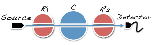
Figure 2: (Color online) Experimental setup to implement the quantum delayed choice. It consists of a Source of two-level atoms, Ramsey zones (R1 and R2), one microwave cavity C, and selective atomic state detectors.

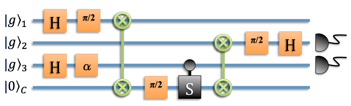
Figure 3: (Color online) Effective circuit corresponding to our proposal to implement QDCE in cavity QED. In this circuit are indicated the Hadamard gate, the Swap gate, and the controlled phase gate. $\pi/2$ indicates the relative phase in atomic states. At the final stage, both the cavity $C$ and the atom $A_{1}$ end in their ground state. While the atom $A_{1}$ is disregarded, the cavity $C$ is now prompt for new sequential operations. The Hadamard gate combined with a $\pi/2$ gate can be achieved through a single controlled operation. The same is true for the SWAP and $\pi/2$ gates.

Initially, the system, as indicated in the circuit of Fig. 3, is in the ground state. In the first step, Rydberg atoms $A_{1}$ and $A_{3}$ (here to be the ancilla) emitted by the source in their ground state, cross the Ramsey zones $R_{1}$ and $R_{2}$ and are prepared in the states $(|g\rangle_{1}+i|e\rangle_{1})/\sqrt{2}$ and $\cos\alpha|g\rangle_{A}+\sin\alpha|e\rangle_{A}$, respectively, according to Eq.(7). Note that this operation, indicated by a Hadamard gate followed by a $\pi/2$ gate in Fig. 3, is achieved through a single controlled operation Eq(4), such that before the first SWAP gate the whole state is:

$$|g,g,,g,0\rangle_{123C} \rightarrow \frac{(|g\rangle_{1}+i|e\rangle_{1})}{\sqrt{2}}|g\rangle_{2}$$

$$\otimes \left(\cos\alpha|g\rangle_{3}+\sin\alpha|e\rangle_{3}\right)|0\rangle_{C}\text{,}$$

where the atom $A_{2}$, indicated in its ground state $|g\rangle_{2},$ is to be the system encoding the WL and PL statistics. The SWAP gate, followed by a $\pi/2$ gate, is accomplished at once by the Hamiltonian Eq.(8) when $A_{1}$ traverses the cavity $C$ and interacts resonantly with the field mode in the vacuum state $|0\rangle_{2}$ with the time interaction adjusted to $gt=\pi/2$:

$$|g\rangle_{1}|g\rangle_{2}\left(\cos\alpha|g\rangle_{3}+\sin\alpha|e\rangle_{3}\right)\frac{(|0\rangle_{C}+|1\rangle_{C})}{\sqrt{2}}\text{.}$$

The next step is the controlled phase gate, which is accomplished when the atom $A_{3}$ interacts off resonantly with the cavity $C$ according to Hamiltonian Eq.(9) with an arbitrary parameter $g^{2}t/\delta=\vartheta$:

$$\frac{1}{\sqrt{2}}|g\rangle_{1}|g\rangle_{2}[\cos\alpha|g\rangle_{3}|0\rangle_{C}+\sin\alpha|e\rangle_{3}|0\rangle_{C}$$

$$+\cos\alpha|g\rangle_{3}|1\rangle_{C}+\sin\alpha\exp(i\vartheta)|e\rangle_{3}|1\rangle_{C}]\text{.}$$

Now, the second SWAP gate between the atom $2$ and cavity $C$ (followed by the $\pi/2$ gate on the path of atom $2$) is achieved in the same way as done previously: atom 2 interacts resonantly with the cavity field, Eq.(8), with $gt=\pi/2$:

$$\frac{1}{\sqrt{2}}|g\rangle_{1}[\cos\alpha|g\rangle_{3}|g\rangle_{2}+\sin\alpha|e\rangle_{3}|g\rangle_{2}$$

$$-i\cos\alpha|g\rangle_{3}|e\rangle_{2}-i\sin\alpha\exp(i\vartheta)|e\rangle_{3}|e\rangle_{2}]|0\rangle_{C}\text{.}$$

in the last step of the circuit, a Hadamard gate is achieved when atom $2$ goes through a Ramsey zone with $\theta=\frac{\pi}{4}$ and $\chi=\pi/2$. Note that the cavity state returns to its initial ground state, allowing a new sequential operation. Therefore, before detection and disregarding both the cavity $C$ and atom $A_{1},$ the final state is

$$|\psi\rangle_{23}=\cos\alpha|p\rangle_{2}|g\rangle_{3}+\sin\alpha|w\rangle_{2}|e\rangle_{3}\text{,}$$

where

$$|p\rangle_{2} = e^{i\frac{\pi}{4}}\frac{(|g\rangle_{2}+i|e\rangle_{2})}{\sqrt{2}}$$

$$|w\rangle_{2} = e^{i\frac{\phi}{2}}\left[\cos\frac{\phi}{2}|g\rangle_{2}-i\sin\frac{\phi}{2}|e\rangle_{2}\right]$$

and $\phi=\frac{\vartheta+\pi}{2}$. The morphing behavior between wave and particle is thus verified by varying the continuous parameter $\alpha$.

Conclusion. We have proposed a feasible experiment to implement a quantum delayed choice experiment (QDCE) in the realm of cavity QED. Our proposal relies on controlled unitary operations, such as the routinely implemented in cavity QED experiments using two-level atoms interacting on and off resonantly with a single mode of a cavity field, plus selective atomic state detectors. Given the technology currently achieved for high Q cavities, in which a photon lifetime reaches $0.1s$ Gleyzes07 , we have disregarded losses both in atomic and cavity field states.

- (1) R. Ionicioiu and D. R. Terno, Phys. Rev. Lett. 107, 230406 (2011).
- (2) J.-S. Tang, Y.-L. Li, X.-Y. Xu, G.-Y. Xiang, C.-F. Li, and G.-C. Guo, Nature Photon. 6, 600 (2012).
- (3) A. Peruzzo, P. Shadbolt, N. Brunner, S. Popescu, and J. L. O’Brien, Science 338, 634 (2012).
- (4) F. Kaiser, T. Coudreau, P. Milman, D. B. Ostrowsky, and S. Tanzilli, Science 338, 637 (2012).
- (5) R. Auccaise, R. M. Serra, J. G. Filgueiras, R. S. Sarthour, I. S. Oliveira, and L. C. Céleri, Phys. Rev. A 85, 032121 (2012).
- (6) S. S. Roy, A. Shukla, and T. S. Mahesh, Phys. Rev. A 85, 022109 (2012).
- (7) J. A. Wheeler, in Mathematical Foundations of Quantum Mechanics, A. R. Marlow, ed. (Academic, New York, 1978).
- (8) S. S. Roy, A. Shukla, and T. S. Mahesh, Phys. Rev. A 85, 022109 (2012).
- (9) J. G. Filgueiras, R. S. Sarthour, A. M. S. Souza, I. S. Oliveira, R. M. Serra, and L. C. Céleri, arXiv:1208.0802 (2012).
- (10) M. O. Scully and M. S. Zubary, Quantum Optics, Cambridge Univ. press, (1997).
- (11) J. M. Raimond, M. Brune, and S. Haroche, Rev. Phys. Mod. 73, 565 (2001).
- (12) J.-S. Tang, Y.-L. Li, C.-F. Li, and G.-C. Guo, arXiv:1204.5304 [quant-ph] (2012).
- (13) R. F. Werner, Phys. Rev. A 40, 4277 (1989).
- (14) S. Gleyzes, S. Kuhr, C. Guerlin, J. Bernu, S. Deléglise, U. B. Hoff, M. Brune, J.-M. Raimond, and S. Haroche, Nature 446, 297 (2007).