Formulation of the Schwinger mechanism in classical statistical field theory

Abstract

In this paper, we show how classical statistical field theory techniques can be used to efficiently perform the numerical evaluation of the non-perturbative Schwinger mechanism of particle production by quantum tunneling. In some approximation, we also consider the back-reaction of the produced particles on the external field, as well as the self-interactions of the produced particles.

• Institut de Physique Théorique (URA 2306 du CNRS)
  CEA/DSM/Saclay, 91191 Gif-sur-Yvette Cedex, France

• High Energy Accelerator Research Organization (KEK)
  1-1 Oho, Tsukuba, Ibaraki 305-0801, Japan

1 Introduction

The Schwinger mechanism [1] (see [2] for a comprehensive review) is a phenomenon by which charged particles, e.g. electron-positron pairs, are produced spontaneously from an external electrical field. This phenomenon is non-perturbative since pairs can be produced even from a static electrical field, something which is forbidden at any finite order of perturbation theory by simple kinematical arguments. It is also a purely quantum phenomenon, whose probability goes to zero in the classical limit $\hbar\to 0$. Loosely speaking, $e^{+}e^{-}$ vacuum fluctuations are promoted to on-shell real particles by picking energy to the electrical field – which can be viewed as a kind of quantum tunneling process.

In Quantum Electrodynamics, the probability for particle production by the Schwinger mechanism is of the order of $\exp(-\pi m^{2}/eE)$, for particles of mass $m$ and electrical charge $e$, in a field $E$. For fields one may realistically create in experiments, and taking even the lightest charged particle, the electron, this probability is so small (mostly due to the fact that the coupling constant $e$ is small) that this phenomenon has remained elusive in all laboratory experiments so far (the typical electrical field necessary to make the production of an electron-positron pair likely is of the order of $E\sim m^{2}/e\sim 10^{18}$ V/m).

The subject of pair production by the Schwinger mechanism is also relevant in the context of Quantum Chromodynamics and strong interactions, since the strong coupling constant $g$ is much larger. It is for instance an important ingredient in hadronization models such as the Lund string model [3], where the breaking of a “string” made of a color electrical field into quark-antiquark pairs leads to meson production. It is also an ingredient in several phenomenological models of heavy ion collisions, e.g. [4, 5, 6, 7, 8, 9].

It may also be a relevant mechanism of particle production in the Color Glass Condensate framework (see [10, 11, 12, 13, 14]), that is commonly used in the description of the first stages of hadronic or nuclear collisions at high energy. In this effective theory, the fast partons –mostly gluons at high energy– of the two colliding projectiles act as a static classical color source. The gluon occupation number, and therefore also this color source, increases with energy. Eventually, when the gluon occupation becomes of order of the inverse strong coupling $1/g^{2}$, nonlinear effects that tame this growth become important – an effect known as gluon saturation [15, 16, 17]. In this regime, the color source corresponding to the fast partons is of order $1/g$, and therefore it creates fields that are themselves of order $1/g$. The probability of pair creation by such a strong field is not suppressed since $gE$ can be large, unlike in QED. In [18], it has been argued that the CGC framework at next-to-leading order (1-loop) includes the contribution of the Schwinger mechanism to particle production.

The Color Glass Condensate provides a semi-classical description of the underlying dynamics: at leading order (tree level), observables are computed by solving classical field equations of motion. This power counting is justified by the large occupation numbers and large fields that characterize the saturation regime, that allow one to neglect the non-commuting nature of the quantum fields and treat them as classical. The color fields obtained at leading order –the Glasma [19, 14]– are non-perturbatively large, of order $1/g$, and can thus lead to a large pair production. At next-to-leading order (1-loop), one can formulate observables in terms of small perturbations of this classical field [20, 21], that obey linearized (and still classical) equations of motion. Equivalently, these 1-loop corrections can be calculated, and resummed, by computing a classical path integral where one sums over a Gaussian ensemble of initial conditions for the classical field encountered at leading order. This approach, sometimes called classical statistical field theory, has been employed in a number of problems in cosmology [22, 23, 24], cold atom physics [25, 26], and more recently in computations related to the thermalization of the quark-gluon plasma in heavy ion collisions [27, 28, 29, 30, 31, 32].

The traditional method of computing the Schwinger mechanism has been to obtain it from the imaginary part of the Heisenberg-Euler Lagrangian [33], which in more modern quantum field theory language corresponds to calculating the imaginary part of the 1-loop effective action. It has also been derived in the framework of kinetic theory [34, 35, 36]. In Refs. [37, 38, 39], the Schwinger mechanism was computed from the Bogoliubov transformation that maps the creation-annihilation operators at $t=+\infty$ onto those at $t=-\infty$. This requires that one solves the linearized equations of motion in order to obtain the time evolution of the mode functions (i.e. modes that start as plane waves in the remote past, and are distorted by their propagation over the external field).

Motivated by the applications of the classical statistical method to the CGC framework, we show in the present paper how the Schwinger mechanism can be calculated in classical statistical field theory, despite being an intrinsically quantum phenomenon. In order to keep the formalism as light as possible, we consider scalar electrodynamics instead of QCD. Note that a similar approach has been used in the case of fermion production in ref. [40, 41, 42], following an idea of ref. [43] to simulate fermions efficiently on a lattice.

In the section 2, we describe the model and discuss two methods of calculating the spectrum of produced particles at leading order; first in a rather standard quantum field theory formulation, and secondly as a classical path integral. In the section 3, we describe the lattice formulation of this calculation in order to evaluate the particle spectrum numerically, and then we compare the results of the classical statistical approach to the results obtained by the direct calculation of the 1-loop diagram, in order to show that they are indeed equivalent. We improve this calculation in the section 4 in order to include the back-reaction of the produced particle pairs on the electrical field. Indeed, this screening effect is crucial for proper energy conservation. The self-interactions among the produced particles, that are crucial for the eventual thermalization of the system, are considered in the section 5. Since the issue of thermalization in classical statistical field theory has been addressed elsewhere, we focus here on the issue of mass renormalization, which plays a crucial role in the Schwinger mechanism due to its extreme sensitivity on the mass of the particles being produced. Finally, the section 6 contains some concluding remarks, while details about the mass renormalization are relegated to the appendix A.

2 Single inclusive spectrum at leading order

2.1 Scalar QED model

Let us consider the case of a complex scalar field $\phi$ with U(1) symmetry, minimally coupled to an Abelian vector field $A^{\mu}$. The vector field may be coupled to an external source $J^{\mu}$ that drives it to a non-perturbatively large value. The classical Lagrangian of this model is

$${\cal L}\equiv-\frac{1}{4}F_{\mu\nu}F^{\mu\nu}+(D_{\mu}\phi)(D^{\mu}\phi)^{*}-m^{2}\phi^{*}\phi-V(\phi\phi^{*})+J^{\mu}_{\rm ext}A_{\mu}$$

$$F^{\mu\nu}=\partial^{\mu}A^{\nu}-\partial^{\nu}A^{\mu}\quad,\quad D^{\mu}\equiv\partial^{\mu}-ieA^{\mu}\;,$$ (1)

where $e$ is the electrical charge of the scalar particles described by the field $\phi$. We have not specified for now the self-interaction potential $V$ of the scalar field, except for the fact that it depends only on the U(1) invariant $\phi\phi^{*}$. A typical example of such a potential would be a quartic interaction,

$$V(\phi\phi^{*})=\frac{\lambda}{4}(\phi\phi^{*})^{2}\;,$$ (2)

where $\lambda$ sets the strength of the self-interactions.

The external source $J^{\mu}_{\rm ext}$ can produce a non-trivial gauge potential, which in turn may produce scalar particles. Assuming that the initial state of the system is the vacuum, the inclusive spectrum of scalar particles is given by the following formula in terms of the 2-point correlation function of the field $\phi$,

$$\frac{dN_{1}}{d^{3}{\boldsymbol{p}}}=\frac{1}{(2\pi)^{3}2E_{\boldsymbol{p}}}\int d^{4}xd^{4}y\;e^{-ip\cdot(x-y)}\;(\square_{x}+m^{2})(\square_{y}+m^{2})\,\big{<}0_{\rm in}\big{|}\phi^{\dagger}(x)\phi(y)\big{|}0_{\rm in}\big{>}\;,$$ (3)

where $E_{\boldsymbol{p}}^{2}\equiv{\boldsymbol{p}}^{2}+m^{2}$. This expression is simply the Lehmann-Symanzik-Zimmermann reduction formula for the expectation value of the number operator $a^{\dagger}({\boldsymbol{p}})a({\boldsymbol{p}})$. Although this form of the reduction formula involves 4-dimensional integrals over the entire space-time, it can also be written in terms of purely spatial integrals thanks to the identity

$$\int\!d^{4}x\,e^{ip\cdot x}\;(\square_{x}+m^{2})\phi(x)=\!\int\!d^{3}{\boldsymbol{x}}\,e^{ip\cdot x}\;\big{[}\dot{\phi}(x^{0},{\boldsymbol{x}})-iE_{\boldsymbol{p}}\phi(x^{0},{\boldsymbol{x}})\big{]}^{x^{0}=+\infty}_{x^{0}=-\infty}\;,$$ (4)

where $[A(x^{0})]^{b}_{a}\equiv A(b)-A(a)$ and the dot denotes a time derivative. Moreover, the lower boundary $x^{0}\to-\infty$ does not contribute since we assume that the initial state is empty. Thus, eq. (3) can also be written as

$$\frac{dN_{1}}{d^{3}{\boldsymbol{p}}} = \lim_{t\to+\infty}\frac{1}{(2\pi)^{3}2E_{\boldsymbol{p}}}\int d^{3}{\boldsymbol{x}}d^{3}{\boldsymbol{y}}\;e^{+i{\boldsymbol{p}}\cdot({\boldsymbol{x}}-{\boldsymbol{y}})}$$ (5)

$$\quad\quad\times\big{<}0_{\rm in}\big{|}(\dot{\phi}^{\dagger}(t,{\boldsymbol{x}})+iE_{\boldsymbol{p}}\phi^{\dagger}(t,{\boldsymbol{x}}))(\dot{\phi}(t,{\boldsymbol{y}})-iE_{\boldsymbol{p}}\phi(t,{\boldsymbol{y}}))\big{|}0_{\rm in}\big{>}\;.$$

On may remove the limit $t\to\infty$ in this formula, and interpret its result as the particle spectrum at the time $t$. However, one has to keep in mind that this interpretation cannot be completely rigorous: strictly speaking, the particles need to be free and on-shell in order for their number to be a well defined concept, which takes an infinite time.

In addition, this formula for the spectrum assumes that the gauge potential vanishes when $t\to+\infty$. However, even if the electrical and magnetic fields are made to vanish in this limit, the gauge potential itself could be a non-zero pure gauge $A^{\mu}\equiv\partial^{\mu}\chi$. In this case, we need to perform in eq. (5) the replacement

$$e^{-i{\boldsymbol{p}}\cdot{\boldsymbol{x}}}\quad\to\quad e^{-i{\boldsymbol{p}}\cdot{\boldsymbol{x}}}\,e^{ie\chi(x)}\;.$$ (6)

(In words, we must gauge transform the free plane waves that are used in the Fourier decomposition of the fields). Note that this replacement is also required in order to have a gauge invariant spectrum. In the particular case where the gauge potential ${\boldsymbol{A}}$ is spatially homogeneous, this substitution can also be written as

$$e^{-i{\boldsymbol{p}}\cdot{\boldsymbol{x}}}\quad\to\quad e^{-i({\boldsymbol{p}}+e{\boldsymbol{A}})\cdot{\boldsymbol{x}}}\;,$$ (7)

and we recognize now the well known difference between the kinetic and canonical momenta

$${\boldsymbol{p}}_{\rm cano}={\boldsymbol{p}}_{\rm kin}+e{\boldsymbol{A}}\;.$$ (8)

By extension, we will also perform this substitution in order to define the particle spectrum in the presence of a homogeneous electrical field (i.e. when the gauge potential is not a pure gauge). Again, one must keep in mind that the concept of particle number in the presence of a non-trivial background field is not rigorously defined, since the particles we are trying to count are not free particles.

2.2 Spectrum at Leading Order

A typical graph contributing to the spectrum is shown in the figure 1.

Figure 1: Generic contribution to the inclusive spectrum of produced scalar particles. The wavy lines represent the photons, while the solid black lines are scalars. The crosses terminating the photon lines represent the source $J^{\mu}_{\rm ext}$.

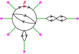
The spectrum can be organized as a triple series expansion, in powers of the electromagnetic coupling $e$, of the self-coupling $\lambda$, and of the external source $J^{\mu}_{\rm ext}$.

When the external source $J^{\mu}_{\rm ext}$ is large, possibly of order $J_{\rm ext}\sim{\cal O}(e^{-1})$, one may expect non-perturbative effects such as the Schwinger mechanism to become important. In order to compute these contributions which are usually non analytic in $e$, it is necessary to treat exactly the external source $J^{\mu}_{\rm ext}$. In the rest of the paper, we call Leading Order the result of this treatment, in which we include all powers of $e$ accompanied by a power of $J^{\mu}_{\rm ext}$, but no further corrections in $e^{2}$ or in $\lambda$. Therefore, the graphs that contribute to the spectrum at leading order are considerably simpler (see the figure 6), since they have only one scalar loop dressed by insertions of a photon directly connected to the external source $J^{\mu}_{\rm ext}$.

Figure 2: One of graphs contributing to the inclusive spectrum at leading order. The leading order consists of all such graphs which have arbitrary number of external lines connected to the external source.

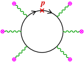
At this level of approximation, one can treat the gauge field attached to the scalar loop is a classical field ${\cal A}^{\mu}$ that obeys the classical Maxwell’s equations,

$$\partial_{\mu}{\cal F}^{\mu\nu}=J^{\nu}_{\rm ext}\;,$$ (9)

and the equation for $\phi$ is linear with respect to quantum fields:

$$({\cal D}_{\mu}{\cal D}^{\mu}+m^{2})\,\phi=0\;,$$ (10)

where ${\cal D}_{\mu}\equiv\partial_{\mu}-ie{\cal A}_{\mu}$ is the covariant derivative constructed with the classical background field. A solution of this equation can be expanded by normal modes as

$$\phi(x)=\int\frac{d^{3}{\boldsymbol{q}}}{(2\pi)^{3}2E_{\boldsymbol{q}}}\left[\varphi_{\boldsymbol{q}}(x)a_{\text{in}}({\boldsymbol{q}})+\varphi_{\boldsymbol{q}}^{*}(x)b_{\text{in}}^{\dagger}({\boldsymbol{q}})\right],$$ (11)

where $a_{\text{in}}({\boldsymbol{q}})$ and $a_{\text{in}}({\boldsymbol{q}})$ are the annihilation operator for particle and antiparticle, respectively, and follow the commutation relations

$$\left[a_{\text{in}}({\boldsymbol{q}}),a_{\text{in}}^{\dagger}({\boldsymbol{q}}^{\prime})\right]=\left[b_{\text{in}}({\boldsymbol{q}}),b_{\text{in}}^{\dagger}({\boldsymbol{q}}^{\prime})\right]=(2\pi)^{3}2E_{\boldsymbol{q}}\delta({\boldsymbol{q}}-{\boldsymbol{q}}^{\prime})\;.$$ (12)

The positive frequency mode function $\varphi_{{\boldsymbol{q}}}(x)$ follows

$$({\cal D}_{\mu}{\cal D}^{\mu}+m^{2})\varphi_{{\boldsymbol{q}}}(x)=0\quad,\quad\lim_{x^{0}\to-\infty}\varphi_{{\boldsymbol{q}}}(x)=e^{-iq\cdot x}\;.$$ (13)

The 2-point correlation function that enters in the spectrum is expressible as follows

$$\big{<}0_{\rm in}\big{|}\phi^{\dagger}(x)\phi(y)\big{|}0_{\rm in}\big{>}_{{}_{\rm LO}}=\int\frac{d^{3}{\boldsymbol{q}}}{(2\pi)^{3}2E_{\boldsymbol{q}}}\;\varphi_{{\boldsymbol{q}}}(x)\varphi_{{\boldsymbol{q}}}^{*}(y)$$ (14)

At this point, the calculation of the scalar particle yield at leading order has been recasted into a purely classical calculation, where one needs to solve the classical equation of motion $({\cal D}_{\mu}{\cal D}^{\mu}+m^{2})\varphi=0$ for each of the scalar mode functions $\varphi_{{\boldsymbol{q}}}$. In the special case of a static electrical field, eqs. (14) are equivalent to the classic result of Schwinger. Note that eqs. (14) do not imply that the particle spectrum at leading order is a classical quantity. Indeed, it is well known in the case of a static electrical field that the particles are produced by a quantum tunneling phenomenon, whose probability goes to zero if $\hbar\to 0$. Instead, eqs. (14) should be viewed as an example of the general property that one-loop quantities can be written as quadratic forms in terms of fields that obey linearized classical equations of motion.

A crucial aspect of this formulation is that these mode functions are specified by retarded boundary conditions in the remote past, where they behave as free plane waves. Using the identity (4) and the fact that in the limit $x^{0}\to-\infty$, we have $\varphi_{{\boldsymbol{q}}}^{*}(x)=e^{iq\cdot x}$, we simply have

$$\int\!d^{4}x\,e^{ip\cdot x}\,(\square_{x}+m^{2})\varphi_{{\boldsymbol{q}}}^{*}(x)=\lim_{x^{0}\to+\infty}\!\int\!d^{3}{\boldsymbol{x}}\,e^{ip\cdot x}\;\big{[}\dot{\varphi}_{{\boldsymbol{q}}}^{*}(x^{0},{\boldsymbol{x}})-iE_{\boldsymbol{p}}\varphi_{{\boldsymbol{q}}}^{*}(x^{0},{\boldsymbol{x}})\big{]}\,.$$ (15)

Thus, as illustrated in the figure 3, the physical interpretation of eqs. (14) is that in order to obtain the spectrum of produced particles, one should start in the remote past with negative energy plane waves (that are equivalent, by crossing symmetry, to having a positive energy antiparticle in the final state), that subsequently evolve over the classical gauge field ${\cal A}^{\mu}$, and are projected at the final time on a positive energy plane wave. The momentum ${\boldsymbol{q}}$ of the incoming plane wave can be interpreted as the momentum of the antiparticle that must be produced along with the observed particle of momentum ${\boldsymbol{p}}$, and therefore should be integrated out in order to obtain the particle spectrum.

Figure 3: Diagrammatic representation of eqs. (14).

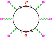
This formulation provides an explicit numerical method for computing the yield at leading order for a general background field (for which it is not possible to solve analytically the equation of motion for $\varphi_{{\boldsymbol{q}}}$): discretize space and solve numerically the classical equation of motion for each momentum ${\boldsymbol{q}}$ of the reciprocal lattice. This is however a computationally expensive method, since this computation scales like the square of the number of lattice points. More precisely, the computation time scales as

$$N_{t}\times N_{\rm latt}^{2}\;,$$ (16)

where $N_{\rm latt}$ is the number of lattice points and $N_{t}$ the number of time-steps used in solving the equations of motion.

2.3 Reformulation as a Gaussian functional integral

It is however possible to formulate the particle spectrum in an alternative way, that allows a more efficient computation based on a Monte-Carlo sampling in a functional space that we shall specify shortly. Since the evolution of the mode functions is causal, knowing them, as well as their first order time derivative, on some Cauchy surface $\Sigma$ (for instance, any surface of constant time $x^{0}$) is sufficient to fully determine their subsequent evolution. To illustrate this, let us consider the following functional

$$G_{xy}[\varphi_{0},\pi_{0}]\equiv\varphi^{*}(x)\varphi(y)$$

$$({\cal D}_{\mu}{\cal D}^{\mu}+m^{2})\,\varphi=0\quad,\quad\varphi(t_{0},{\boldsymbol{x}})=\varphi_{0}({\boldsymbol{x}})\;,\;\dot{\varphi}(t_{0},{\boldsymbol{x}})=\pi_{0}({\boldsymbol{x}})\;.$$ (17)

$G_{xy}[\varphi_{0},\pi_{0}]$ is the product at the points $x$ and $y$ of the classical solution $\varphi$ whose initial conditions at the time $t_{0}$ are given by the functions $\varphi_{0}({\boldsymbol{x}}),\pi_{0}({\boldsymbol{x}})$. Let us introduce a Gaussian average over initial values $\varphi_{0}({\boldsymbol{x}}),\pi_{0}({\boldsymbol{x}})$ as

$$\big{<}\mathcal{O}\left[\varphi_{0},\pi_{0}\right]\big{>}\equiv\int[D\varphi_{0}D\pi_{0}]\;W[\varphi_{0},\pi_{0}]\;\mathcal{O}[\varphi_{0},\pi_{0}],$$ (18)

with $W[\varphi_{0},\pi_{0}]$ being the Gaussian kernel which is characterized by the following 2-point correlation functions :

$$\big{<}\varphi_{0}^{*}({\boldsymbol{x}})\varphi_{0}({\boldsymbol{y}})\big{>} =\frac{1}{2}\int\frac{d^{3}{\boldsymbol{q}}}{(2\pi)^{3}2E_{\boldsymbol{q}}}\;\Big{[}\varphi_{{\boldsymbol{q}}}^{*}(t_{0},{\boldsymbol{x}})\varphi_{{\boldsymbol{q}}}(t_{0},{\boldsymbol{y}})+\varphi_{{\boldsymbol{q}}}(t_{0},{\boldsymbol{x}})\varphi_{{\boldsymbol{q}}}^{*}(t_{0},{\boldsymbol{y}})\Big{]}$$

$$\big{<}\pi_{0}^{*}({\boldsymbol{x}})\pi_{0}({\boldsymbol{y}})\big{>} =\frac{1}{2}\int\frac{d^{3}{\boldsymbol{q}}}{(2\pi)^{3}2E_{\boldsymbol{q}}}\;\Big{[}\dot{\varphi}_{{\boldsymbol{q}}}^{*}(t_{0},{\boldsymbol{x}})\dot{\varphi}_{{\boldsymbol{q}}}(t_{0},{\boldsymbol{y}})+\dot{\varphi}_{{\boldsymbol{q}}}(t_{0},{\boldsymbol{x}})\dot{\varphi}_{{\boldsymbol{q}}}^{*}(t_{0},{\boldsymbol{y}})\Big{]}$$ (19)

$$\big{<}\varphi_{0}({\boldsymbol{x}})\pi_{0}({\boldsymbol{y}})\big{>} =0\;.$$

From these definitions, the following equation is trivially obtained:

$$\big{<}G_{xy}[\varphi_{0},\pi_{0}]\big{>}=\frac{1}{2}\int\frac{d^{3}{\boldsymbol{q}}}{(2\pi)^{3}2E_{\boldsymbol{q}}}\;\Big{[}\varphi_{{\boldsymbol{q}}}(x)\varphi_{{\boldsymbol{q}}}^{*}(y)+\varphi_{{\boldsymbol{q}}}(y)\varphi_{{\boldsymbol{q}}}^{*}(x)\Big{]}\;.$$ (20)

Further using Eq. (14), we get

$$\big{<}G_{xy}[\varphi_{0},\pi_{0}]\big{>}=\frac{1}{2}\big{<}0_{\rm in}\big{|}\phi^{\dagger}(x)\phi(y)+\phi(y)\phi^{\dagger}(x)\big{|}0_{\rm in}\big{>}_{{}_{\rm LO}}\;.$$ (21)

In other words, this procedure gives almost the expectation value we need in order to compute the particle spectrum, except for the ordering between the two field operators. In the form (5) of the reduction formula, the two field operators are evaluated at equal times. Therefore, $\phi^{\dagger}(x)$ and $\phi(y)$ commute, but not $\dot{\phi}^{\dagger}(x)$ and $\phi(y)$. In fact, if we used the expectation value (21) in the LSZ formula, we would get the expectation value of the operator $(a^{\dagger}({\boldsymbol{p}})a({\boldsymbol{p}})+a({\boldsymbol{p}})a^{\dagger}({\boldsymbol{p}}))/2$ instead of $a^{\dagger}({\boldsymbol{p}})a({\boldsymbol{p}})$. This discrepancy is easy to fix by using the commutation relation (12). One can obtain the leading order spectrum by calculating the expectation value (21), and then by subtracting $V/2$ particles where $V$ is the volume of the system. More precisely,

$$\left.\frac{dN_{1}}{d^{3}{\boldsymbol{p}}}\right|_{{}_{\rm LO}}=-\frac{V}{2}+\int[D\varphi_{0}D\pi_{0}]\;W[\varphi_{0},\pi_{0}]\;F_{\boldsymbol{p}}[\varphi_{0},\pi_{0}]\;,$$ (22)

where

$$F_{\boldsymbol{p}}[\varphi_{0},\pi_{0}]\equiv\frac{1}{(2\pi)^{3}2E_{\boldsymbol{p}}}\left|\Phi_{\boldsymbol{p}}[\varphi_{0},\pi_{0}]\right|^{2}$$

$$\Phi_{\boldsymbol{p}}[\varphi_{0},\pi_{0}]=\lim_{x^{0}\to+\infty}\int d^{3}{\boldsymbol{x}}\;e^{ip\cdot x}\;\big{[}\dot{\varphi}(x^{0},{\boldsymbol{x}})-iE_{\boldsymbol{p}}\varphi(x^{0},{\boldsymbol{x}})\big{]}$$

$$({\cal D}_{\mu}{\cal D}^{\mu}+m^{2})\,\varphi=0\quad,\quad\varphi(t_{0},{\boldsymbol{x}})=\varphi_{0}({\boldsymbol{x}})\;,\;\dot{\varphi}(t_{0},{\boldsymbol{x}})=\pi_{0}({\boldsymbol{x}})\;.$$ (23)

It is easy to check that if we carry out this procedure in the vacuum (i.e. with ${\cal D}_{\mu}=\partial_{\mu}$ in the equation of motion of the scalar field), we obtain $dN_{1}/d^{3}{\boldsymbol{p}}=0$. The subtraction of the term $V/2$ is crucial for that.

This reformulation of the spectrum at leading order can be illustrated diagrammatically as follows,

$$\raise-28.45274pt\hbox to85.35826pt{\leavevmode\resizebox{85.35826pt}{}{\includegraphics{sp_LO1}}}\;=\;\underbrace{\raise-14.22636pt\hbox to85.35826pt{\leavevmode\resizebox{85.35826pt}{}{\includegraphics{sp_LO2-2}}}}_{W[\varphi_{0},\pi_{0}]}\;\otimes\;\underbrace{\raise-14.22636pt\hbox to85.35826pt{\leavevmode\resizebox{85.35826pt}{}{\includegraphics{sp_LO2-1}}}}_{F_{\boldsymbol{p}}[\varphi_{0},\pi_{0}]}\;.$$ (24)

The new representation amounts to slicing the scalar loop at a certain time $t_{0}$, and to assign to the functional $F_{p}[\varphi_{0},\pi_{0}]$ the time evolution for $x^{0}>t_{0}$, and to the Gaussian distribution $W[\varphi_{0},\pi_{0}]$ the part of the evolution at $x^{0}<t_{0}$. The Gaussian average over the fields $\varphi_{0},\pi_{0}$ is the “glue” that reconstructs the loop, since it amounts to connecting pairwise the two open endpoints of $F_{p}[\varphi_{0},\pi_{0}]$. Note that the choice of the time $t_{0}$ is not important, since the left hand side does not depend on this choice. In fact, instead of slicing the loop at a fixed time $t_{0}$, the separation in two factors could have been made on any locally space-like surface. In practical implementations, it is best to perform the separation at a time $t_{0}$ such that the distribution $W[\varphi_{0},\pi_{0}]$ is easy to compute.

Note that random elements of the Gaussian ensemble defined by eq. (19) can be generated by writing

$$\varphi_{0}({\boldsymbol{x}}) = \int\frac{d^{3}{\boldsymbol{q}}}{(2\pi)^{3}2E_{\boldsymbol{q}}}\;\big{[}c_{\boldsymbol{q}}\,\varphi_{{\boldsymbol{q}}}(t_{0},{\boldsymbol{x}})+d_{\boldsymbol{q}}\,\varphi_{{\boldsymbol{q}}}^{*}(t_{0},{\boldsymbol{x}})\big{]}$$

$$\pi_{0}({\boldsymbol{x}}) = \int\frac{d^{3}{\boldsymbol{q}}}{(2\pi)^{3}2E_{\boldsymbol{q}}}\;\big{[}c_{\boldsymbol{q}}\,\dot{\varphi}_{{\boldsymbol{q}}}(t_{0},{\boldsymbol{x}})+d_{\boldsymbol{q}}\,\dot{\varphi}_{{\boldsymbol{q}}}^{*}(t_{0},{\boldsymbol{x}})\big{]}\;,$$ (25)

where $c_{\boldsymbol{q}}$ and $d_{\boldsymbol{q}}$ are random complex Gaussian distributed numbers, whose 2-point correlations are

$$\big{<}c_{\boldsymbol{q}}c_{{\boldsymbol{q}}^{\prime}}^{*}\big{>}=\big{<}d_{\boldsymbol{q}}d_{{\boldsymbol{q}}^{\prime}}^{*}\big{>}=(2\pi)^{3}E_{\boldsymbol{q}}\delta({\boldsymbol{q}}-{\boldsymbol{q}}^{\prime})$$

$$\big{<}c_{\boldsymbol{q}}c_{{\boldsymbol{q}}^{\prime}}\big{>}=\big{<}d_{\boldsymbol{q}}d_{{\boldsymbol{q}}^{\prime}}\big{>}=\big{<}c_{\boldsymbol{q}}d_{{\boldsymbol{q}}^{\prime}}\big{>}=\big{<}c_{\boldsymbol{q}}d_{{\boldsymbol{q}}^{\prime}}^{*}\big{>}=0\;.$$ (26)

2.4 Numerical cost

Eq. (22) may at first appear to be a drawback compared to eq. (14) since we have replaced an ordinary integral by a functional integration. However, let us assume that the mode function $\varphi_{{\boldsymbol{q}}}$ is known (or at least easily computable) at the initial time $t_{0}$. This is for instance the case when the background field ${\cal A}^{\mu}$ is vanishing for $x^{0}<t_{0}$. Then, one can estimate the functional integral by doing a Monte-Carlo sampling of the Gaussian ensemble defined by eqs. (19), i.e. by generating random functions of the form (25) and by solving the equation of motion for each of these samples. The computational time of this method would be of the order of

$$N_{\rm samples}\times N_{\rm latt}\times\big{(}N_{\rm latt}+N_{t}\big{)}\;,$$ (27)

where $N_{\rm samples}$ is the number of samples used in the Monte-Carlo evaluation of the functional integral. Note that the first term, proportional to $N_{\rm latt}^{2}$, is due to the fact that in eq. (25) there is a sum over ${\boldsymbol{q}}$ at each position ${\boldsymbol{x}}$. This has to be repeated for each sample, but needs to be done only at the initial time $t_{0}$. This Monte-Carlo method of evaluating the particle spectrum is less costly than the direct method provided that

$$N_{\rm samples}\ll N_{\rm latt}\quad,\quad N_{\rm samples}\ll N_{t}\;.$$ (28)

The first condition is obvious: if one uses a number of samples which is larger than the number of independent mode functions, then one would be better off using the direct method (since it would give the exact leading order answer, for a lesser computational effort). The second condition implies that the computation is dominated by the resolution of the equations of motion rather than the evaluation of the initial conditions.

3 Lattice numerical evaluation

3.1 Lattice setup

In the two formulations, (14) or (22), one needs to solve the linearized equation of motion $({\cal D}_{\mu}{\cal D}^{\mu}+m^{2})\varphi=0$ for the propagation of a scalar field on top of some background electromagnetic potential ${\cal A}_{\mu}$. There are only a few known examples of background fields for which this equation of motion can be solved analytically. For a generic background field, one can only solve this equation numerically.

Actual computations are done by discretizing space on a lattice. We consider a finite box of volume $L_{x}\times L_{y}\times L_{z}$ and divide it into a $N_{\rm latt}\equiv N_{x}\times N_{y}\times N_{z}$ lattice. Space points are labeled as

$${\boldsymbol{x}}\equiv(n_{x}a_{x},n_{y}a_{y},n_{z}a_{x})\quad(n_{x}=1,\cdots,N_{x};\ n_{y}=1,\cdots,N_{y};\ n_{z}=1,\cdots,N_{z})\;,$$ (29)

with lattice spacing $a_{x}=L_{x}/N_{x}$, etc. We impose the periodic boundary conditions, e.g. $\varphi(x,y,z)=\varphi(x+L_{x},y,z)$, and the momenta are given by

$$p_{i}=\frac{2\pi k_{i}}{L_{i}}\hskip 20.0pt(i=x,y,z)\;,$$ (30)

where the $k_{i}$ are integers, taken in the range

$$k_{i}=-\frac{N_{i}}{2}+1,\cdots,0,\cdots,\frac{N_{i}}{2}\qquad(i=x,y,z)\;,$$ (31)

where we have assumed that the lattice sizes $N_{i}$ are even.

On the lattice, differentiation with respect to space is replaced by finite differences. Let us introduce the forward difference

$$\nabla_{i}^{+}\varphi({\boldsymbol{x}})\equiv\frac{1}{a_{i}}\left[\varphi({\boldsymbol{x}}+a_{i}\hat{n}_{i})-\varphi({\boldsymbol{x}})\right]\;,$$ (32)

where the vector $\hat{n}_{i}$ is the displacement by one lattice spacing in the spatial direction $i$. Similarly, the backward difference is

$$\nabla_{i}^{-}\varphi({\boldsymbol{x}})\equiv\frac{1}{a_{i}}\left[\varphi({\boldsymbol{x}})-\varphi({\boldsymbol{x}}-a_{i}\hat{n}_{i})\right]\;.$$ (33)

By “integration by parts”, the forward difference is transformed to the backward difference :

$$\sum_{\boldsymbol{x}}\big{[}\nabla_{i}^{+}f({\boldsymbol{x}})\big{]}g({\boldsymbol{x}})=-\sum_{\boldsymbol{x}}f({\boldsymbol{x}})\Big{[}\nabla_{i}^{-}g({\boldsymbol{x}})\Big{]}\;.$$ (34)

(Notice that there is no boundary term because of the periodic boundary condition.) In words, this means that $\nabla_{i}^{-}$ and $\nabla_{i}^{+}$ are mutually adjoint. Since it is desirable to have a self-adjoint Laplacian operator, it is convenient to define it by a mix of forward and backward derivatives

$$\Delta\equiv\sum_{i=x,y,z}\nabla_{i}^{-}\nabla_{i}^{+}\;.$$ (35)

The discrete plane waves $\exp(i{\boldsymbol{p}}\cdot{\boldsymbol{x}})$ are eigenfunctions of this operator, with eigenvalues

$$-E_{k_{x},k_{y},k_{z}}^{2}\equiv-2\sum_{i=x,y,z}\frac{\sin^{2}(\frac{\pi k_{i}}{N_{i}})}{a_{i}^{2}}\;.$$ (36)

When considering scalar QED, the local $U(1)$ gauge invariance can be preserved on the lattice by defining the forward covariant derivative as

$$D_{i}^{+}\varphi({\boldsymbol{x}})\equiv\frac{1}{a_{i}}\left[e^{iea_{i}A_{i}({\boldsymbol{x}})}\varphi({\boldsymbol{x}}+a_{i}\hat{n}_{i})-\varphi({\boldsymbol{x}})\right]\;,$$ (37)

Under a gauge transformation

$$\varphi(t,{\boldsymbol{x}}) \longrightarrow e^{ie\theta(t,{\boldsymbol{x}})}\varphi(t,{\boldsymbol{x}})$$

$$A_{0}(t,{\boldsymbol{x}}) \longrightarrow A_{0}(t,{\boldsymbol{x}})-\dot{\theta}(t,{\boldsymbol{x}})$$

$$A_{i}(t,{\boldsymbol{x}}) \longrightarrow A_{i}(t,{\boldsymbol{x}})-\nabla_{i}^{+}\theta(t,{\boldsymbol{x}})\;,$$ (38)

$D_{i}^{+}\varphi(t,{\boldsymbol{x}})$ is transformed in the same way as $\varphi(t,{\boldsymbol{x}})$ :

$$D_{i}^{+}\varphi(t,{\boldsymbol{x}})\;\longrightarrow\;e^{ie\theta(t,{\boldsymbol{x}})}D_{i}^{+}\varphi(t,{\boldsymbol{x}})\;.$$ (39)

One can write a gauge invariant discretized Lagrangian density for the complex scalar fields as follows

$$\mathcal{L}_{\text{matter}}=\left(D_{0}\phi\right)^{*}\left(D_{0}\phi\right)-\sum_{i=x,y,z}\left(D_{i}^{+}\phi\right)^{*}\left(D_{i}^{+}\phi\right)-m^{2}\phi^{*}\phi-V\left(\phi^{*}\phi\right)\;.$$ (40)

In deriving the discretized classical equation of motion, one should note that the forward covariant derivative is the adjoint of the backward covariant derivative $D_{i}^{-}$,

$$D_{i}^{-}\varphi({\boldsymbol{x}})=\frac{1}{a_{i}}\left[\varphi({\boldsymbol{x}})-e^{-iea_{i}A_{i}({\boldsymbol{x}}-a_{i}\hat{n}_{i})}\varphi({\boldsymbol{x}}-a_{i}\hat{n}_{i})\right]\;.$$ (41)

One obtains

$$\Big{(}D_{0}^{2}-\sum_{i=x,y,z}D_{i}^{-}D_{i}^{+}+m^{2}\Big{)}\,\varphi+V^{\prime}(\varphi^{*}\varphi)\,\varphi=0\;.$$ (42)

(Here the equation is written with the self-interaction term, but in the evaluation of the spectrum at leading order we need only the linear part of the equation.) It is convenient to choose the temporal gauge $A^{0}=0$, so that $D_{0}=\partial_{0}$ in the equation of motion.

3.2 Numerical results

In order to demonstrate that the classical statistical simulation (CSS) can indeed describe the Schwinger mechanism at leading order, we consider a simple situation which can be handled easily by the direct quantum field theory method. The self-coupling $\lambda$ is set to zero in this leading order computation, and we take a spatially homogeneous background electrical field in the $z$ direction (and no magnetic field), that we switch on at the time $x^{0}=0$. In this case, thanks to the translational invariance of the problem, the direct evaluation of eq. (14) is not very expensive and will be used as a benchmark against which we compare the CSS results.

The parameters of the lattice simulation are $N_{x}=N_{y}=32$, $N_{z}=256$ (we need more lattice spacings in the direction of the electrical field), corresponding to physical sizes $L_{x}=L_{y}=50$, and $L_{z}=30$ respectively. The mass is taken to be $m=0.1$, the electrical charge is $e=1$ and the electrical field is switched on at $x^{0}=0$ and its value is $E=1$ (alternatively, one may view $eE$ as arbitrary and all the other dimensionful quantities as being quoted in units of $\sqrt{eE}$, that has the dimension of a mass). 1024 field configurations were used in order to sample the Gaussian ensemble defined in eqs. (25).

In the figure 4 we show the longitudinal momentum distribution of the produced scalar particles, at several times shortly after the electrical field has been switched on. The dots represent the result of the classical statistical approach and the solid lines are the direct QFT calculation.

Figure 4: Comparison of the $p_{z}$ spectrum between the classical statistical simulation and the direct 1-loop QFT calculation in the case of a constant electrical field.

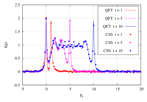
The agreement between the two approaches is very good, and the differences compatible with the expected statistical error given the number of samples used in the CSS approach. In particular, the intricate oscillatory pattern of this spectrum, which results from quantum interference phenomena, is well reproduced in the CSS method. This shows very concretely how 1-loop quantum effects can be reformulated in terms of purely classical objects.

The time evolution of the $p_{z}$ spectrum is rather transparent: particles are produced with a small $p_{z}$ by quantum tunneling, and later they are accelerated in the direction of the electrical field; hence the expansion of the spectrum towards larger (positive, because we are considering only particles –not antiparticles–) values of $p_{z}$. One can indeed see on the figure 4 that this expansion is linear in time, in good agreement with a constant acceleration $eE$ (which is equal to 1 with our choice of units) of the particles in the $+z$ direction. Similarly, the comparison of the $p_{\perp}$ spectra obtained in the two approaches, in the figure 5, show a good agreement within statistical errors.

Figure 5: Comparison of the $p_{\perp}$ spectrum between the classical statistical simulation and the direct 1-loop QFT calculation in the case of a constant electrical field.

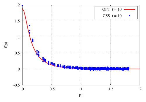
The shape of the transverse momentum spectrum is very different from that of the longitudinal momentum distribution. Roughly speaking, the produced particles originate from virtual pairs (i.e. vacuum fluctuations) that can have a momentum in any direction. Then, their longitudinal momentum $p_{z}$ increases linearly in time due to the electrical field, while their transverse momentum is not affected.

To close this section, we also show the energy density and electrical current density carried by the produced particles, as a function of time, in the figure 6.

Figure 6: Energy density and electrical current density carried by the produced particles. In the left plot, the light blue band indicates the energy density of the electrical field.

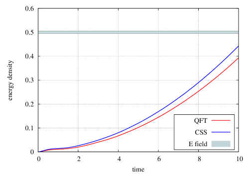
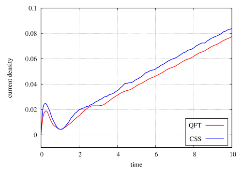
The energy density of the produced particles increases steadily with time, and at some point it will overcome the energy density of the background electrical field. When this occurs, the simple calculation done in this section, where the back-reaction of the produced particles on the gauge field is neglected, becomes certainly insufficient. In particular, the total energy present in the system is not conserved at this level of approximation, because of the uninterrupted production of scalar particles, shown in the left plot of the figure 6. One could in fact use this as a criterion for deciding when the one loop approximation ceases to be valid: it should be improved when the energy carried by the produced particles becomes of the same order of magnitude as the energy density carried by the electrical field. From the left plot of 6, we expect this breakdown to occur as early as $t\sim 10$.  This is also corroborated by the behavior of the electrical current carried by the produced particles. Because this current acts as a source in the Maxwell’s equations that control the gauge potential, it can alter the background electrical field when it becomes too large.

4 Back-reaction effects

In the previous section, we have seen that the plain 1-loop calculation of the spectrum of produced particles is bound to break down after some time, because this approximation violates energy conservation. What is missing is the back-reaction of the produced scalar particles on the electrical field, which has the effect of screening this field, which eventually will put an end to the production of particles [46, 47].

Taking into account the back-reaction means that the source of the electromagnetic field is not just the external source $J^{\mu}_{\rm ext}$, but also includes the contribution of the scalar field $\phi$ to the electromagnetic current,

$$j^{0}(x) = ie\left[\phi^{*}(x)\dot{\phi}(x)-\dot{\phi}^{*}(x)\phi(x)\right]$$

$$j^{i}(x) = ie\left[\phi^{*}(x)D_{i}^{+}\phi(x)-\left(D_{i}^{+}\phi(x)\right)^{*}\phi(x)\right]\;,$$ (43)

written here with lattice discrete spatial derivatives. In the gauge $A^{0}=0$, the Maxwell’s equation for the vector potential read

$$\nabla^{i}_{-}\dot{A}^{i}=J^{0}_{\rm ext}+j^{0}$$

$$\ddot{A}^{i}+(\nabla^{i}_{+}\nabla^{j}_{-}-\delta^{ij}\nabla_{+}\cdot\nabla_{-})\,A^{j}=J^{i}_{\rm ext}+j^{i}\;.$$ (44)

The first of the two equations (44) is Gauss’s law. It is automatically satisfied if $A^{i}$ obeys the second equation, and $J^{\mu}$ is conserved,

$$\dot{J}^{0}=\nabla^{i}_{-}J^{i}\;,$$ (45)

which, in turn, is the case if the scalar field $\phi$ obeys the equation of motion.

Figure 7: Left: topologies included when solving simultaneously the equations of motion of the scalar field $\phi$ and the Maxwell’s equations with the induced current, from some given boundary conditions $\varphi_{0},\pi_{0}$ at the initial time $t_{0}$. Right: QFT topologies when we perform a Gaussian average of the left graph over the Gaussian ensemble (19), with $j^{\mu}$ replaced by the ensemble average $\big{<}j^{\mu}\big{>}$ in Maxwell’s equations.

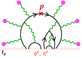
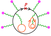
Diagrammatically, solving simultaneously the equation of motion of the scalar field $\phi$ and Maxwell’s equations, starting from some initial condition $\varphi_{0}({\boldsymbol{x}}),\pi_{0}({\boldsymbol{x}})$ at the time $t_{0}$, amounts to resumming graphs such as the one represented in the left part of the figure 7. All the graphs are made of a principal scalar line, to which the measured particle of momentum ${\boldsymbol{p}}$ is attached. To this line are attached a number of photons. These photons can either be attached to the external current $J^{\mu}_{\rm ext}$, or to the induced current, i.e. to another scalar line. These secondary scalar lines can themselves be decorated by photons, etc…

Averaging the functional of $\varphi_{0},\pi_{0}$ obtained by this procedure over the Gaussian distribution of initial conditions defined by (19) amounts to reconnecting pairwise all the hanging scalar lines in the graph of the figure 7. Although all the topologies obtained when doing this were indeed present in the original quantum field theoretical formulation of the particle spectrum, some of them are miscalculated by the classical statistical simulation. This because in the CSS all propagators are retarded, while they are Feynman propagators in the field theoretical calculation. However, when we reconnect together the two scalars that enter in the same instance of the induced current, the classical statistical approach reproduces exactly the QFT value of that loop. This amounts to replacing the induced current $j^{\mu}$ in Maxwell’s equation by its ensemble average,

$$j^{\mu}\quad\to\quad\left<j^{\mu}\right>\;.$$ (46)

By doing this, one obtains all the graphs such as the one represented in the right part of the figure 7, where the scalar loops represented in orange originate from the use of $\left<j^{\mu}\right>$ in the right hand side of Maxwell’s equations. Although this is not manifest on this example, these scalar loops can themselves be dressed by an arbitrary number of photon insertions, whose other endpoint can either be the external current $J^{\mu}_{\rm ext}$ or another instance of the ensemble averaged induced source.

Let us now show some numerical results that illustrate the effect of the back reaction. First, in the figure 8, we display the electrical current density (left) and the resulting electrical field (right).

Figure 8: Time evolution of the electrical current density and of the resulting electrical field when the back-reaction is taken into account.

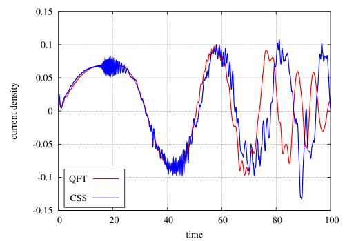
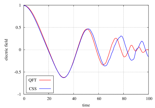
There in an inflection in the growth of the current at a time $t\approx 10$, which roughly corresponds to the moment when the energy carried by the produced particles becomes comparable to the energy stored in the electrical field. Simultaneously, the electrical field decreases and even changes sign periodically, while the amplitude of its oscillations decrease to zero. Consequently, the production of particles slows down and effectively stops after some time (when the probability of particle creation, of the order of $\exp(-\pi m^{2}/eE)$, becomes too small).

Figure 9: Illustration of the polarization phenomenon that leads to the reduction of the electrical field when the back-reaction is taken into account.

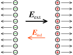
It is rather easy to understand why the induced electrical field is opposite in direction to the externally field, as illustrated in the figure 9. Indeed, after having been produced, the positive charges are accelerated in the direction of the external field and the negative charges in the opposite direction. This charge separation acts like capacitor plates, that create an induced field oriented from the positive to the negative charges. The induced electrical field thus counteracts the effect of the external field.

In the left plot of the figure 10, we see that the expansion of the $p_{z}$ spectrum towards the right is no longer linear in time, a direct consequence of the decreasing electrical field which is no longer providing a constant acceleration to the produced particles. In fact the plot on the right of the figure 10 shows that for slightly larger times, the shift towards the right of the $p_{z}$ spectrum comes to a halt, and is replaced by a shift to the left. Obviously, this happens when the electrical field has changed sign, around $t\approx 30$. After the $p_{z}$ spectrum moves into the negative momentum region, its value undergoes a rapid increase. This is because particles which have been created earlier pass through the zero-momentum region and stimulate the subsequent particle production (Bose-enhancement). At the same time, the $p_{z}$ spectrum starts to show an oscillatory pattern. This is due to an interference between the fields of the previously produced particles and of the newly produced particles [38]. It is remarkable that the CSS method can describe this intricate pattern of peaks, that are purely quantum effects.

Figure 10: Left: evolution at short times of the $p_{z}$ spectrum of the produced scalar particles. Right: evolution of the $p_{z}$ spectrum at intermediate times.

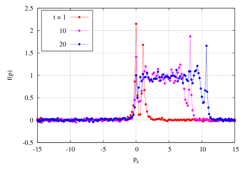
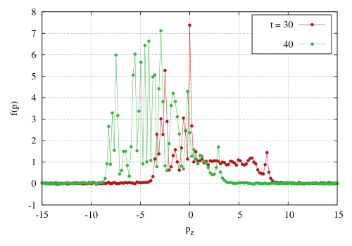
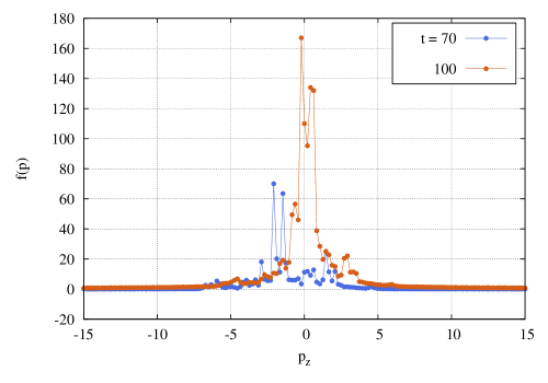
At even larger times, when the electrical field has become small, the $p_{z}$ distribution becomes roughly centered around $p_{z}=0$, as one can see from the plot on the left of the figure 11. Because the electric field has changed its sign for several times, the spectrum has gone through several stages of Bose-enhancement and is now much larger than its value at early times.

Figure 11: Left: evolution of the $p_{z}$ spectrum over longer time scales. Right: decomposition of the energy of the system between fields and particles.

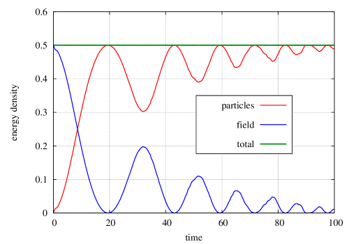
Finally, one can also check that the inclusion of the back-reaction effects cure the main problem of the plain 1-loop calculation, i.e. the energy conservation. In the plot on the right of the figure 11, we have represented the energy density carried by the produced particles, the energy density carried by the electromagnetic fields, and the sum of the two contributions. We observe a transfer into particles of the energy initially stored in the electrical field, while the total energy remains constant.

5 Self-interactions and mass renormalization

So far, all the results we have shown have neglected the self-interactions of the scalar fields. This means that after the external electrical field has been “neutralized” by the produced particles, their distribution is frozen and ceases to evolve. In particular, it has no way to thermalize. The effect of these self-interactions has been studied in the classical statistical framework employed here, where it is rather straightforward to take into account since it just amounts to adding a non-linear term in the equation of motion of the classical scalar fields,

$$\Big{(}D_{0}^{2}-\sum_{i=x,y,z}D_{i}^{-}D_{i}^{+}+m^{2}\Big{)}\,\varphi+\frac{\lambda}{2}(\varphi^{*}\varphi)\,\varphi=0\;,$$ (47)

written here for a quartic self-interaction. In the slightly simpler example of a real scalar field theory, it has been shown that these nonlinearities lead to the isotropization and thermalization of the momentum distribution of the particles.

Figure 12: Left: topologies included when solving simultaneously the equations of motion of the scalar field $\phi$ with self-interactions and the Maxwell’s equations with the induced current, from some given boundary conditions $\varphi_{0},\pi_{0}$ at the initial time $t_{0}$. Right: topologies obtained after the Gaussian average over the initial conditions $\varphi_{0},\pi_{0}$, with $\big{<}j^{\mu}\big{>}$ as the source term in Maxwell’s equations.

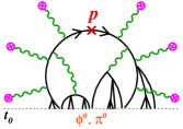
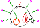
Diagrammatically, including the self-interactions in the classical equation of motion of the scalar fields changes the figure 7 into the figure 12. In particular, the Gaussian average over the initial conditions for the scalar field can now produce loop corrections such as (but not only) tadpoles.

Our goal in this section in not to reproduce previous results on thermalization in classical statistical simulations, but to stress the complication due to mass renormalization, which is crucial when dealing with a tunneling phenomenon such as the Schwinger mechanism. The main issue is that the probability of particle production by quantum tunneling is extremely sensitive to the value of the mass of the scalar particles, since its square enters in the exponential $\exp(-\pi m^{2}/eE)$. However, when we include the nonlinear term in the equation of motion of the scalar field and we average over its initial conditions, we resum some loop corrections that are ultraviolet divergent. In a lattice simulation, they are regularized by the lattice spacing, but provide a potentially large renormalization of the mass that will alter significantly the production of particles by the Schwinger mechanism. The worst offenders are the tadpole corrections, that have a quadratic dependence on the inverse lattice spacing.

Figure 13: $p_{z}$ spectrum of the produced scalar particles at $t=10$, in the non self-interacting case ($\lambda=0$) and the self-interacting case ($\lambda=1$), without and with mass renormalization. The two horizontal bands indicate the values of $\exp(-\pi m^{2}/eE)$ for $m^{2}=0.01$ and $m^{2}=0.27$ (see the text for an explanation of these values).

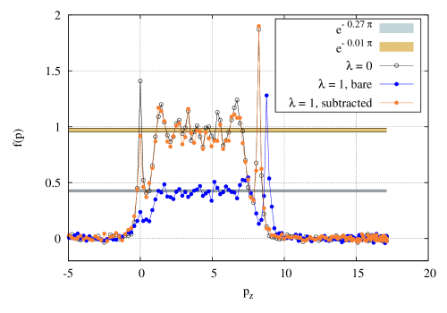
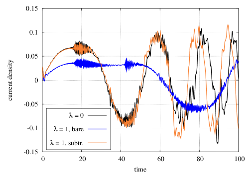
This problem is illustrated in the figure 13. The black curve, which is almost overlapping with the orange curve, shows the spectrum of produced particles (at $t=10$, i.e. shortly after the external field has been switched on) without self-interactions (i.e. with a coupling constant $\lambda=0$). The (bare) mass in the Lagrangian, and hence in the classical equation of motion, is $m=0.1$. This curve should be compared to the blue curve, where the same computation has been performed with a nonzero self-coupling $\lambda=1$, and the same value of the bare mass. We see that the particle yield has been considerably reduced. As we shall argue, this is a consequence of the fact that these two computations correspond to two different values of the renormalized mass. This is an unphysical effect that should be fixed. Indeed, one expects that the self-interactions among the scalar fields alter their long time evolution (and in particular play a crucial role in their thermalization), but should have little physical effects at short times. This issue is also visible in the two plots of the figure 14, where the computation at $\lambda=0$ and the bare computation at $\lambda=1$ lead to very different results, even at short times.

Figure 14: Time evolution of the electrical current density (left) and of the electrical field (right). Curves are shown for the non self-interacting case ($\lambda=0$), and for the self-interacting case ($\lambda=1$), without and with mass renormalization.

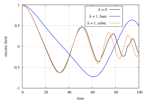
As explained in the appendix A, one can remove the quadratic divergence coming from the tadpoles by adding a mass counterterm $\delta m^{2}$ in the equation of motion for the classical scalar field. This mass counterterm is space-time independent, and can thus be computed once for all at the initial time. We define it by

$$\delta m^{2}\equiv-\lambda\left<\varphi^{*}(0,{\boldsymbol{x}})\varphi(0,{\boldsymbol{x}})\right>\;,$$ (48)

which is directly given by eq. (19) and is obviously independent of the external electrical field. With the value of the self-coupling $\lambda=1$ that we are using, we have $\lambda\left<\varphi^{*}(0,{\boldsymbol{x}})\varphi(0,{\boldsymbol{x}})\right>=0.26$, which is why the calculation done without any mass renormalization gives a yield that is well reproduced by $\exp(-\pi m^{2}/eE)$ with $m^{2}=0.26+0.01=0.27$ (see the figure 13). In the figure 13, we also show the $p_{z}$ spectrum obtained when this counterterm is added to the classical equation of motion. Now, we see that the particle yield is back at the level expected for a renormalized mass $m_{{}_{R}}^{2}=0.01$. Similarly, the figure 14 shows that this mass renormalization cures the unphysical effect of the self-interactions at short times.

6 Conclusions

Motivated by recent works on thermalization in heavy ion collisions using classical statistical field theory, in which one computes 1-loop quantum corrections by performing a Gaussian average over the initial condition of a purely classical field, we have applied the same method to the calculation of the Schwinger mechanism of particle production in an external electrical field.

We have first shown that, at leading order (i.e. at 1-loop), the spectrum of particles produced by the Schwinger mechanism can be expressed as a path integral over classical fields that have a Gaussian ensemble of initial conditions. The 2-point correlation function that characterizes this Gaussian distribution is uniquely determined by the propagator of small fluctuations on top of the external field. This representation of the spectrum is exact at 1-loop, and is a mere rewriting of the original quantum field theory result. Moreover, this formulation of the spectrum leads to a very efficient method for the numerical evaluation of the spectrum on a lattice.

Then, by promoting the gauge potential to a dynamical variable, this formulation makes easy the inclusion of the back-reaction effects that are important for the physical consistency of the model. Indeed, the charged particles that are produced via the Schwinger mechanism tend to screen the applied external field, thereby reducing progressively their production rate. This back-reaction is essential for the conservation of total energy (particles + electromagnetic field).

In the last section, we have studied the possibility of taking into account the self-interactions of the produce charged particles, which is an essential ingredient for their eventual thermalization. In the classical statistical approach, they can be simply included by keeping the non-linear interaction term in the classical equation of motion for the field. However, since the Schwinger mechanism is very sensitive to the value of the mass of the particles, it is important to take proper steps in order to renormalize the mass: the naive (i.e. without any mass renormalization) inclusion of the self-interactions leads to an unphysical –lattice spacing dependent– reduction of the charged particle yield, because the self-interactions produce large corrections to the mass. The main correction to the mass is a quadratic ultraviolet divergence that comes from tadpole corrections. We have shown that it can be systematically subtracted in the classical statistical framework by adding a mass counterterm in the classical field equation of motion.

To close this paper, we would like to digress with a remark regarding the applicability of the classical statistical approach to the calculation of observables. The example considered in this paper, as well as other quantities previously considered in the literature, is an inclusive observable. This means that it measures the expectation value of a certain operator (here the particle number operator) in the final state of the system, without putting any constraints on this final state. This is the reason why these observables can be expressed in terms of fields that obey retarded boundary conditions, which in turn are amenable to a computation in terms of a Gaussian average over their initial conditions. Very little is known about exclusive observables, whose definition veto certain final states. The archetypal example of this kind of observable would be the probability of producing a specific number of charged particles, which obviously excludes any final state that does not contain the expected number of particles. In some examples, it has been shown that exclusive observables can be expressed at leading order in terms of classical fields that obey non-retarded boundary conditions (e.g. fields that are constrained both at $t=-\infty$ and at $t=+\infty$). At least on the surface, it seems very implausible that such an observable can be obtained by a classical statistical simulation where one performs an average over the initial conditions of the classical field.

Appendix A Tadpoles in classical statistical field theory

In this appendix, we show how to deal with the quadratic divergences that arise from the tadpoles when we keep the self-interactions in a classical statistical simulation. In this appendix, we disregard the coupling of the scalars to the gauge fields, since our purpose is to discuss an issue related to the scalar self-coupling. Moreover, in order to keep the notations simple, we use continuum notations in this appendix. In practical applications to an actual lattice computation, all the integrals would become discrete sums.

Let us illustrate the issue in the case of the simple calculation of the expectation value of the field operator itself, $\big{<}\phi(x)\big{>}$. Before we go further, it is useful to recall the Green’s formula that relates the classical field $\varphi(x)$ to its initial value at $x^{0}=0$:

$$\varphi(x)=-\frac{\lambda}{2}\int_{y^{0}>0}\!\!\!d^{4}y\;G_{{}_{R}}^{0}(x,y)\,\varphi^{*}(y)\varphi^{2}(y)+\int_{y^{0}=0}\!\!\!d^{3}{\boldsymbol{y}}\;G_{{}_{R}}^{0}(x,y)\stackrel{{\scriptstyle\leftrightarrow}}{{\partial^{0}_{y}}}\varphi(0,{\boldsymbol{y}})\;,$$ (49)

where $G_{{}_{R}}^{0}(x,y)$ is the free retarded Green’s function of the Dalembertian operator. By iterating the interaction term, one sees that the functional dependence of $\varphi$ with respect to its initial condition can be represented as a sum of tree diagrams, of the form:

$$\varphi(x)=\raise-27.0301pt\hbox to170.71652pt{\hfil\leavevmode\resizebox{170.71652pt}{}{\includegraphics{green-tree}}}+\cdots$$ (50)

In this equation, we have represented the terms that arise up to the second order in the coupling. The vertical dotted line symbolizes the initial time surface $y^{0}=0$, and the red circles the initial value of the field $\varphi$ at this initial time. The average over the initial field is a Gaussian average; it can be done diagrammatically by introducing the following objects

(51)

where the green dot represents the central value of the Gaussian ensemble, and the green link represents its 2-point correlation function. When we apply these diagrammatic rules to the expectation value of the field operator, we obtain the following contributions

$$\left<\phi(x)\right>=\raise-123.76949pt\hbox to284.52756pt{\hfil\leavevmode\resizebox{284.52756pt}{}{\includegraphics{avg-tree}}}$$ (52)

In this diagrammatic representation, the green lines and dots represent the average over the initial condition, while the black lines are genuine (retarded) propagators coming from the subsequent time evolution. The first line is the sum of tree level contributions, the second line is the 1-loop contribution, etc.. The tree level contribution (first line) is nothing but the classical field whose initial condition at $x^{0}=0$ is the central value of the Gaussian ensemble, $\varphi_{0}$. We see that in the classical statistical approach, this classical solution is corrected by an infinite set of loop corrections.

The tadpoles are the loops that have the strongest dependence on the ultraviolet cutoff. Before going further, it is worth clarifying an important point: it is not obvious a priori that the tadpole-like subgraphs that appear in the diagrams of eq. (52) are identical to the usual tadpoles encountered in Feynman’s perturbation theory. Let us demonstrate that they are in fact equal. By using the Green’s formula (49), the tadpoles of eq. (52) can be expressed as

$$= \!\!\int\limits_{y^{0},z^{0}=0}\!\!d^{3}{\boldsymbol{y}}d^{3}{\boldsymbol{z}}\;\Big{[}G_{{}_{R}}^{0}(x,y)\stackrel{{\scriptstyle\leftrightarrow}}{{\partial^{0}}}_{y}\Big{]}\Big{[}G_{{}_{R}}^{0}(x,z)\stackrel{{\scriptstyle\leftrightarrow}}{{\partial^{0}}}_{z}\Big{]}\left<\varphi(0,{\boldsymbol{y}})\varphi(0,{\boldsymbol{z}})\right>$$ (53)

$$= \!\!\int\limits_{y^{0},z^{0}=0}\!\!d^{3}{\boldsymbol{y}}d^{3}{\boldsymbol{z}}\int\frac{d^{4}pd^{4}q}{(2\pi)^{8}}\frac{1}{(p^{2}+ip^{0}\epsilon)(q^{2}+iq^{0}\epsilon)}$$

$$\qquad\qquad\times\Big{[}e^{-ip\cdot(x-y)}\stackrel{{\scriptstyle\leftrightarrow}}{{\partial^{0}}}_{y}\Big{]}\Big{[}e^{-iq\cdot(x-z)}\stackrel{{\scriptstyle\leftrightarrow}}{{\partial^{0}}}_{z}\Big{]}\left<\varphi(0,{\boldsymbol{y}})\varphi(0,{\boldsymbol{z}})\right>$$

$$= \int\frac{d^{3}{\boldsymbol{k}}}{(2\pi)^{3}2k}\;.$$

In the second line, we have replaced the retarded propagators by their Fourier representation. Then, a straightforward calculation, using eqs. (19), leads to the final expression – which is indeed the usual vacuum tadpole. Given the combinatorics for connecting a $\varphi$ and a $\varphi^{*}$ in the product $\varphi^{*}\varphi^{2}$, each tadpole will arise with a prefactor $\lambda$ in the expansion of eq. (52), which is also the right coupling and symmetry factor.

It is possible to subtract all the tadpoles that arise during the time evolution by adding a mass counterterm $\delta m^{2}$ in the classical equation of motion, that becomes

$$\left(\square+m^{2}+\delta m^{2}\right)\varphi+\frac{\lambda}{2}\varphi^{*}\varphi^{2}=0\;.$$ (54)

The effect of this counterterm in the equation of motion is to insert in its solution a mass counterterm in every place where a tadpole is allowed to appear. It therefore adds the following contributions to eq. (52)

$$\delta\left<\varphi(x)\right>=\raise-78.24507pt\hbox to170.71652pt{\hfil\leavevmode\resizebox{170.71652pt}{}{\includegraphics{ct-eom}}}$$ (55)

where the red cross denotes the mass counterterm. The outcome is that the tadpoles are systematically cancelled by this procedure if one tunes the counterterm to precisely cancel the quadratic divergence of the tadpole,

$$\delta m^{2}+\lambda\int\frac{d^{3}{\boldsymbol{k}}}{(2\pi)^{3}2k}<\infty\;.$$ (56)

Eq. (56) only specifies the divergent part of the mass counterterm; it also has a finite part that should be adjusted in order to have the desired renormalized mass. Note also that the inclusion of this counterterm in the equation of motion only subtracts the quadratic divergences, possibly leaving a residual logarithmic dependence on the lattice spacing.

References

- [1] J. Schwinger, Phys. Rev. 82, 664 (1951).
- [2] G.V. Dunne, arXiv:hep-th/0406216, published in ”From fields to strings”, ed. M. Shifman et al., vol. 1, 445 (2004).
- [3] B. Andersson, G. Gustafson, G. Ingelman, T. Sjostrand, Phys. Rept. 97, 31 (1983).
- [4] A. Casher, H. Neuberger, S. Nussinov, Phys. Rev. D 20 179 (1979).
- [5] N.K. Glendenning, T. Matsui, Phys. Rev. D 28, 2890 (1983).
- [6] T.S. Biro, H.B. Nielsen, J. Knoll, Nucl. Phys. B 245, 449 (1984).
- [7] K. Kajantie, T. Matsui, Phys. Lett. B 164, 373 (1985).
- [8] G. Gatoff, A.K. Kerman, T. Matsui, Phys. Rev. D 36, 114 (1987).
- [9] R.C. Wang, C.Y. Wong, Phys. Rev. D 38, 348 (1988).
- [10] E. Iancu, A. Leonidov, L.D. McLerran, Lectures given at Cargese Summer School on QCD Perspectives on Hot and Dense Matter, Cargese, France, 6-18 Aug 2001, hep-ph/0202270.
- [11] E. Iancu, R. Venugopalan, Quark Gluon Plasma 3, Eds. R.C. Hwa and X.N. Wang, World Scientific, hep-ph/0303204.
- [12] T. Lappi, Int. J. Mod. Phys. E20, 1 (2011).
- [13] F. Gelis, E. Iancu, J. Jalilian-Marian, R. Venugopalan, Ann. Rev. Part. Nucl. Sci. 60, 463 (2010).
- [14] F. Gelis, arXiv:1211.3327 [hep-ph].
- [15] L.V. Gribov, E.M. Levin, M.G. Ryskin, Phys. Rept. 100, 1 (1983).
- [16] A.H. Mueller, J-W. Qiu, Nucl. Phys. B 268, 427 (1986).
- [17] J.P. Blaizot, A.H. Mueller, Nucl. Phys. B 289, 847 (1987).
- [18] K. Fukushima, F. Gelis, T. Lappi, Nucl. Phys. A 831, 184 (2009).
- [19] T. Lappi, L.D. McLerran, Nucl. Phys. A 772, 200 (2006).
- [20] F. Gelis, R. Venugopalan, Nucl. Phys. A 776, 135 (2006).
- [21] F. Gelis, T. Lappi, R. Venugopalan, Phys. Rev. D 78, 054019 (2008).
- [22] D. Polarski, A.A. Starobinsky, Class. Quant. Grav. 13, 377 (1996).
- [23] D.T. Son, hep-ph/9601377.
- [24] R. Micha, I.I. Tkachev, Phys. Rev. D 70, 043538 (2004).
- [25] A.A. Norrie, A Classical Field Treatment of Colliding Bose-Einstein Condensates, PhD thesis, University of Otago, New Zealand (2005).
- [26] A.A. Norrie, R.J. Ballagh, C.W. Gardiner, Phys. Rev. Lett. 94, 040401 (2005).
- [27] K. Dusling, T. Epelbaum, F. Gelis, R. Venugopalan, Nucl. Phys. A 850, 69 (2011).
- [28] T. Epelbaum, F. Gelis, Nucl. Phys. A 872, 210 (2011).
- [29] K. Dusling, T. Epelbaum, F. Gelis, R. Venugopalan, Phys. Rev. D 86, 085040 (2012).
- [30] J. Berges, S. Scheffler, S. Schlichting, D. Sexty, Phys. Rev. D 85, 034507 (2012).
- [31] J. Berges, S. Schlichting, Phys. Rev. D 87, 014026 (2013).
- [32] J. Berges, S. Schlichting, D. Sexty, Phys. Rev. D 86, 074006 (2012).
- [33] W. Heisenberg, H. Euler, Z. Phys. 98, 714 (1936).
- [34] S.M. Schmidt, D. Blaschke, G. Ropke, S.A. Smolyansky, A.V. Prozorkevich, V.D. Toneev, Int. J. Mod. Phys. E 7, 709 (1998).
- [35] S.M. Schmidt, D. Blaschke, G. Ropke, A.V. Prozorkevich, S.A. Smolyansky, V.D. Toneev, Phys. Rev. D 59, 094005 (1999).
- [36] D.B. Blaschke, V.V. Dmitriev, G. Ropke, S.A. Smolyansky, Phys. Rev. D 84, 085028 (2011).
- [37] N. Tanji, Annals Phys. 324, 1691 (2009).
- [38] N. Tanji, Annals Phys. 325, 2018 (2010).
- [39] N. Tanji, Phys. Rev. D 83, 045011 (2011).
- [40] F. Hebenstreit, J. Berges, D. Gelfand, Phys. Rev. D 87, 105006 (2013).
- [41] P.M. Saffin, A. Tranberg, JHEP 1202, 102 (2012).
- [42] P.M. Saffin, A. Tranberg, JHEP 1107, 066 (2011).
- [43] Sz. Borsanyi, M. Hindmarsh, Phys. Rev. D 79, 065010 (2009).
- [44] V. Dinu, T. Heinzl, A. Ilderton, Phys. Rev. D 86, 085037 (2012).
- [45] T.W.B. Kibble, Phys. Rev. 138, B740 (1965).
- [46] Y. Kluger, J.M. Eisenberg, B. Svetitsky, F. Cooper, E. Mottola, Phys. Rev. D 45, 4659 (1992).
- [47] S.P. Gavrilov, D.M. Gitman, Phys. Rev. Lett. 101, 130403 (2008).
- [48] G. Aarts, J. Smit, Phys. Lett. B 393, 395 (1997).
- [49] G. Aarts, J. Smit, Nucl. Phys. B 511, 451 (1998).