Estimation of consistent parameter sets for continuous-time nonlinear systems using occupation measures and LMI relaxations

Abstract

Obtaining initial conditions and parameterizations leading to a model consistent with available measurements or safety specifications is important for many applications. Examples include model (in-)validation, prediction, fault diagnosis, and controller design. We present an approach to determine inner- and outer-approximations of the set containing all consistent initial conditions/parameterizations for nonlinear continuous-time systems. These approximations are found by occupation measures that encode the system dynamics and measurements, and give rise to an infinite-dimensional linear program. We exploit the flexibility and linearity of the decision problem to incorporate uncertain-but-bounded and pointwise-in-time state and output constraints, a feature which was not addressed in previous works. The infinite-dimensional linear program is relaxed by a hierarchy of LMI problems that provide certificates in case no consistent initial condition/parameterization exists. Furthermore, the applied LMI relaxation guarantees that the approximations converge (almost uniformly) to the true consistent set. We illustrate the approach with a biochemical reaction network involving unknown initial conditions and parameters.

1 Introduction

The computation of guaranteed inner- and outer-approximations of consistent parameter sets of uncertain dynamical systems is important for many applications including model-based analysis and verification, system identification, model (in-)validation and controller design [15, 1, 18, 17].

We consider the derivation of such approximations for polynomial systems subject to unknown-but-bounded (or error-in-variables) data, e. g. measurements. Different methods are available in literature to address this problem. For discrete-time systems, for instance interval analysis methods, e. g. [8], or relaxation-based methods, e. g. [26, 21, 3, 4] can be employed. However, both approaches are not directly applicable to continuous-time systems without additional assumptions. For instance in [6] it was assumed that the time-derivatives of the states are available as measurements, therefore, resulting in a steady-state problem similar to [11].

One possibility to address continuous-time systems with the mentioned methods is by discrete-time approximations, e. g. obtained by numerical integration. However, due to the discretization error the consistent parameter sets of continuous-time and discrete-time model do not necessarily overlap and, thus, wrong conclusions with respect to model validity are possible [22]. A common approach to limit the discretization error relies on higher-order Taylor approximations resulting in verified integration methods [19, 9, 16, 13, 2, 20], but again the results typically depend on the discretization error.

A more direct approach uses McCormick relaxations or differential inequalities, see [24] and references therein). However, deriving the needed tight state bounds can be difficult.

Methods using barrier certificates and sum-of-squares (SOS) polynomials [18, 17, 1] allow the continuous-time dynamics to be considered directly without numerical integration. However, only few converse results for these, i. e. existence of barrier certificates, are known. Furthermore, to the best of our knowledge, no results with respect to approximations of consistent parameter sets exist so far.

The main contribution of this work is the use of occupation measures [14] to derive guaranteed polynomial inner- and outer-approximations of the consistent parameter sets for continuous-time nonlinear systems based on results presented in [7, 10, 12]. The reformulation in terms of occupation measures leads to a linear but infinite-dimensional decision problem. However, its relaxation using truncated moment matrices and their dual SOS polynomials is a finite-dimensional convex problem. One particular feature of the employed relaxation is the (almost uniform) asymptotic convergence of the approximations to the true consistent parameter set. Another advantage is that the continuous-time dynamics are completely encoded in the decision problem and, thus, no numerical integration is necessary. Furthermore, we exploit the flexibility and linearity of the decision problem to incorporate uncertain-but-bounded and pointwise-in-time state and output constraints, a feature which was not addressed in previous works.

This contribution is structured as follows. In Section 2 we formalize the problem setup, in particular, the considered system class, the description of the uncertain data and the desired properties of the approximations. To obtain constraints for a convex optimization problem, we reformulate in Section 3 the polynomial continuous-time dynamics in terms of occupation measures. In Section 4, we adapt this approach to the consistent parameter estimation problem, which is reformulated as an infinite-dimensional linear programming problem. Its solution is approached numerically with a hierarchy of finite-dimensional semi-definite programs. We show how to derive outer- and inner-approximations, as well as certificates of inconsistency. The approach is demonstrated in Section 5 while its advantages and computational issues are discussed in Section 6.

2 Problem Formulation

In this section we state the problem of set-based parameter estimation for continuous-time nonlinear systems of the following form

$$\dot{x}(t) =f\bigl{(}t,x(t)\bigr{)},\qquad x(t_{0})=x_{0},$$ (1a)

$$y(t) =h\bigl{(}x(t)\bigr{)}.$$ (1b)

Here $t\in[0,1]$ is the time, the states are denoted by $x\in\mathbb{R}^{n_{x}}$ and the outputs by $y\in\mathbb{R}^{n_{y}}$. Note that the terminal time is set to one without loss of generality, after a suitable time-scaling of the dynamics. Initial conditions (at $t=0$) are denoted by $x_{0}$. We assume the vector field $f:\mathbb{R}\times\mathbb{R}^{n_{x}}\rightarrow\mathbb{R}^{n_{x}}$ and $h:\mathbb{R}\times\mathbb{R}^{n_{x}}\rightarrow\mathbb{R}^{n_{y}}$ to be polynomial maps. To simplify notation, we denote the state vector at time $t_{k}\in[0,1]$ by $x_{k}=x(t_{k})$.

Note that time-invariant parameters $p\in\mathbb{R}^{n_{p}}$ can be included in (1) by defining states with constant dynamics $\forall\,i\in 1,\ldots,n_{p}$:

$$\dot{x}_{i}=f_{i}\bigl{(}t,x(t)\bigr{)}=0,\quad\text{where }p_{i}:=x_{i}(0).$$ (2)

That is, the state vector $x$ contains $n_{x}-n_{p}$ true dynamic variables and $n_{p}$ constant parameters. The parameter values are then given by the initial conditions of the corresponding variables $x_{i}$. This formulation unifies the tasks of initial condition and parameter estimation, and also simplifies the notation and analysis using occupation measures and moment relaxations (see next sections).

We assume that constraints on the states, output measurements and initial conditions (including the parameters) are given by polynomial inequalities $g(\cdot)\geq 0$. We rewrite the output constraints $g_{y}\bigl{(}y(t)\bigr{)}\geq 0$ as state constraints using the polynomial output map, i. e. $g_{y}\bigl{(}h(t,x)\bigr{)}\geq 0$.

Let $m_{x}$ time-independent constraints on the states be given in the form $x(t)\in\mathcal{X},\forall\,t\in\left[0,1\right]$ with

$$\mathcal{X}\coloneqq\Bigl{\{}x:\ g_{x,i}\bigl{(}x\bigr{)}\geq 0,\ \forall\,i=1,\ldots,m_{x}\Bigr{\}}\subset\mathbb{R}^{n_{x}}.$$ (3)

We additionally assume that we have a finite set of $m_{t}$ distinct measurements at time points $t_{k},k=0,\ldots,m_{t}-1$, such that: $0=t_{0}<t_{1}<\cdots<t_{m_{t}-1}=1$. These time points include both the measurements of the output $y(t_{k})$ and a priori information on the set of parameters and initial conditions. For each time point $t_{k}$, let the constraints on the states be given in the form $x_{k}\in\mathcal{X}_{k},k=0,\ldots,m_{t}-1$ with

$$\mathcal{X}_{k}\coloneqq\Bigl{\{}x:\ g_{x_{k},i}\bigl{(}x\bigr{)}\geq 0,\ \forall\,i=1,\ldots,m_{x_{k}}\Bigr{\}}\subseteq\mathcal{X}$$ (4)

Using this information, we want to estimate the consistent initial conditions and parameters.

In the following, we denote the admissible state trajectory (an absolutely continuous function of time) of (1) starting at fixed $x_{0}$ with $x(t|x_{0})$, i. e.

$$x(t|x_{0})=x_{0}+\int_{0}^{t}f\bigl{(}\tau,x(\tau)\bigr{)}\,d\tau.$$ (5)

Using (5), we define the set of consistent initial conditions $\mathcal{X}_{0}^{\ast}$ based on the set of consistent trajectories as follows:

$$\mathcal{X}_{0}^{\ast}\coloneqq\Bigl{\{}x_{0}:\exists x(t|x_{0})\text{\ s.\,t.\ }$$

$$x(t|x_{0})\in\mathcal{X},\ \forall\,t\in[0,T]\text{\ and\ }$$ (6)

$$x(t_{k}|x_{0})\in\mathcal{X}_{k},\ \forall\,k=0,\ldots,m_{t}-1\Bigr{\}}.$$

With these notations, we can state the following problem:

Problem 1 (Consistent parameter estimation)

Find inner-approximations $\mathcal{I}$ and outer-approximations $\mathcal{O}$ of consistent initial conditions (parameters) such that ${\mathcal{I}}\subseteq\mathcal{X}_{0}^{\ast}\subseteq\mathcal{O}$.

For many applications such as model validation and fault detection, it is sufficient to determine if the set $\mathcal{X}_{0}^{\ast}$ is empty or not, we therefore state the following related problem:

Problem 2 (Certificate of inconsistency)

If $\mathcal{X}_{0}^{\ast}$ is empty, find a certificate of emptiness.

Consistency of a single initial condition $x_{0}$ can easily be checked numerically by solving equation (5). However, to determine the complete set $\mathcal{X}_{0}^{\ast}$ is in general difficult, e. g. due to the involved nonlinearities and nonconvexities. We use occupation measures (see Section 3) and convex relaxations to derive the outer-approximation $\mathcal{O}$ based on [7]. The basic idea to find the inner-approximation $\mathcal{I}$ is to determine guaranteed enclosures of initial conditions that violate some constraints, cf. Section 4 and [10]. Note that the inner-approximation $\mathcal{I}$ is given by the complement in $\mathcal{X}$ of the union of these enclosures.

In the next section, we describe how to deal with the continuous-time dynamics and state constraints using occupation measures. This enables us to derive convex optimization problems that are used to determine the inner and outer-approximations.

3 Occupation Measures and Liouville’s Equation

The crucial idea we employ in this work is to reformulate the parameter estimation problem in terms of occupation measures. This has two main advantages. First, it allows us to consider an entire distribution (or measure) of initial conditions and parameter values and not just single points. Second, linear relationships encoding the nonlinear dynamics (i. e. trajectories) of the system link these initial measures with corresponding measures at the intermediate time-points for which measurement data are available.

In [7] and the references therein, occupation measures were used to estimate the region of attraction. Here we first review this approach, before we extend it for parameter estimation in Section 4. We show that unknown-but-bounded state constraints at intermediate time points, not considered in [7], can be handled easily. This is achieved by partitioning the occupation measure w.r.t. a partitioning of the time interval, cf. Section 4. To determine the unknown occupation measures, a convex problem is derived. Albeit infinite-dimensional, the convex problem can be solved efficiently by a hierarchy of finite-dimensional relaxations [7, 10, 12].

3.1 Occupation measures

Let $M(\mathcal{A})$ denote the set of finite Borel measures supported on the set $\mathcal{A}$, which can be interpreted as elements of the dual space $C(\mathcal{A})^{\prime}$, i. e. as bounded linear functionals acting on the set of continuous functions $C(\mathcal{A})$. Let ${P}(\mathcal{A})$ denote the set of probability measures on $\mathcal{A}$, i. e. those measures $\mu$ of ${M}(\mathcal{A})$ which are nonnegative and normalized to $\mu(\mathcal{A})=1$.

Now assume that the initial condition $x_{0}$ is not precisely known, but that it can be interpreted as a random variable whose distribution is described by a probability measure $\mu_{0}\in{P}(\mathcal{X})$. We define the occupation measure

$$\mu(\mathcal{A}\times\mathcal{B}):=\int_{\mathcal{T}}\int_{\mathcal{X}}I_{\mathcal{A}\times\mathcal{B}}(t,x(t|x_{0}))\mu_{0}(dx_{0})\,dt$$

for all subsets $\mathcal{A}\times\mathcal{B}$ in the Borel $\sigma$-algebra of subsets of $\mathcal{T}\times\mathcal{X}$, where $\mathcal{T}\subset\mathbb{R}$ is a time interval and $x(t|x_{0})$ is as in (5). Here, $I_{\mathcal{A}}(x)$ is the indicator function of the set $\mathcal{A}$, which is equal to one if $x\in\mathcal{A}$, and zero otherwise.

Note that $\mu\in{P}(\mathcal{T}\times\mathcal{X})$ is a probability measure, and that the terminology occupation measure is motivated by the observation that the value $\int_{\mathcal{T}}\mu(dt,\mathcal{B})=\mu(\mathcal{T}\times\mathcal{B})$ is equal to the total time the trajectory spends in the set $\mathcal{B}\subset\mathcal{X}$. In addition, note that $\mu$ encodes the system trajectories, in the sense that if $v\in{C}^{\infty}(\mathcal{T}\times\mathcal{X};{\mathbb{R}})$ is a smooth test function, and $\mu_{0}=\delta_{x_{0}}$ is the Dirac measure at $x_{0}$, integration of $v$ w.r.t. $\mu$ amounts to time integration along the system trajectory starting at $x_{0}$:

$$\langle v,\mu\rangle:=\int_{\mathcal{T}}\int_{\mathcal{X}}v(t,x)\mu(dt,dx)=\int_{\mathcal{T}}v\bigl{(}t,x(t|x_{0})\bigr{)}\,dt.$$

The occupation measure $\mu$ can be disintegrated as $\mu(\mathcal{A}\times\mathcal{B})=\int_{\mathcal{A}}\mu_{k}(\mathcal{B}|t)\,dt$ where conditional $\mu_{k}$ is a stochastic kernel, in the sense that for every fixed $t\in\mathcal{T}$, $\mu_{k}(dx|t)$ is a probability measure on $\mathcal{X}$ describing the distribution of the state $x$ at time $t_{k}$, and for every $\mathcal{B}\in\mathcal{X}$, $t\mapsto\mu_{k}(\mathcal{B}|t)$ is a measurable function on $\mathcal{T}$.

On the one hand, the introduced measures allow us to consider the whole set of initial conditions ($\mu_{0}$). On the other hand, it allows a reformulation of the nonlinear dynamics (1a) as a linear equation which only depends on the occupation measures ($\mu$, $\mu_{t_{k}}$), as shown next.

3.2 Liouville’s equation

With these notations, for all sufficiently regular test functions $v\in C^{1}(\mathcal{T}\times\mathcal{X};{\mathbb{R}})$ and $\mathcal{T}:=[0,1]$, it holds that

$$\int_{\mathcal{X}}v(1,x)\mu_{1}(dx)-\int_{\mathcal{X}}v(0,x)\mu_{0}(dx)=\int_{\mathcal{T}}\int_{\mathcal{X}}\frac{d}{dt}\,v\bigl{(}t,x(t|x_{0})\bigr{)}\mu_{0}(dx_{0}).$$ (7)

The right-hand-side of the above equation can be rewritten

$$\int_{\mathcal{T}}\int_{\mathcal{X}}\Bigl{(}\frac{\partial}{\partial t}v\bigl{(}t,x(t|x_{0})\bigr{)}+\mathrm{grad}\>v\bigl{(}t,x(t|x_{0})\bigl{)}\cdot f\bigl{(}t,x(t|x_{0})\bigr{)}\Bigr{)}\mu_{0}(dx_{0})\,dt$$

$$= \int_{\mathcal{T}}\int_{\mathcal{X}}\left(\frac{\partial}{\partial t}v(t,x)+\mathrm{grad}\>v(t,x)\cdot f(t,x)\right)\mu(dt,dx).$$

To simplify notation, we introduce the Liouville operator ${\mathcal{L}}:{C}^{1}(\mathcal{T}\times\mathcal{X})\to{C}(\mathcal{T}\times\mathcal{X})$ as ${\mathcal{L}}v:=\frac{\partial v}{\partial t}+\mathrm{grad}\>v\cdot f$ and its adjoint ${\mathcal{L}}^{\prime}:{C}(\mathcal{T}\times\mathcal{X})^{\prime}\to{C}^{1}(\mathcal{T}\times\mathcal{X})^{\prime}$ such that $\langle{\mathcal{L}}v,\mu\rangle=\langle v,{\mathcal{L}}^{\prime}\mu\rangle$ for all $v\in{C}^{1}(\mathcal{T}\times\mathcal{X})$, i.e. ${\mathcal{L}}^{\prime}\mu:=-\frac{\partial\mu}{\partial t}-\mathrm{div}(\mu f).$

With these notations, equation (7) can be written concisely as

$$\langle{\mathcal{L}}v,\mu\rangle=\langle v,\delta_{1}\mu_{1}\rangle-\langle v,\delta_{0}\mu_{0}\rangle$$ (8)

for all $v\in{C}^{1}(\mathcal{T}\times\mathcal{X})$, where $\delta_{0}$ and $\delta_{1}$ refers to $t=0$ and $t=1$, respectively. Equivalently, in the sense of distributions, we can write

$${\mathcal{L}}^{\prime}\mu=\delta_{1}\mu_{1}-\delta_{0}\mu_{0}.$$ (9)

Equation (9) is Liouville’s equation and is also called the continuity equation in statistical physics or fluid mechanics.

Whereas the function $x\in{C}(\mathcal{T}\times\mathcal{X})$ satisfies the nonlinear ordinary differential equation (1a), the occupation measure $\mu\in{P}(\mathcal{T}\times\mathcal{X})$ satisfies Liouville’s equation (9), which is a linear partial differential equation (PDE) in the space of probability measures.

Note that as the initial conditions are not known, the measures are unknown as well. In the next sections we derive an optimization problem that allows us to determine the unknown measures.

3.3 Estimating the region of attraction

In [7] it was proved that the region of attraction $\mathcal{X}_{0}^{\ast}$, defined as the set of initial conditions $x_{0}$ consistent with the dynamics (1a) and the constraints $x(t)\in\mathcal{X}$, $t\in\mathcal{T}$ and a constraint $\mathcal{X}_{1}$ at $t=1$, is the support of the measure $\mu_{0}$ solving the infinite-dimensional linear programming (LP) problem

$$\begin{array}[]{ll}\sup&\langle 1,\mu_{0}\rangle\\ \mathrm{s.t.}&\hat{\mu}_{0}+\mu_{0}=\lambda,\\ &{\mathcal{L}}^{\prime}\mu+\delta_{0}\mu_{0}-\delta_{1}\mu_{1}=0,\\ &\hat{\mu}_{0}\geq 0,\>\mu_{0}\geq 0,\>\mu_{1}\geq 0,\>\mu\geq 0,\end{array}$$ (10)

where $\lambda$ is the Lebesgue measure restricted to $\mathcal{X}$, i. e. the standard $n_{x}$-dimensional volume. The supremum in (10) is w.r.t. measures $\hat{\mu}_{0}\in{P}(\mathcal{X})$, $\mu_{0}\in{P}(\mathcal{X})$, $\mu_{1}\in{P}(\mathcal{X})$ and $\mu\in{P}(\mathcal{T}\times\mathcal{X})$. Note that the slack measure $\hat{\mu}_{0}$ results from the inequality $\mu_{0}\leq\lambda$ as further explained in [7]. The above LP problem has a dual LP

$$\inf \langle v_{0},\lambda\rangle$$

$$\mathrm{s.t.} \begin{array}[t]{lr}v_{0}(x)\geq 0,&\forall\,x\in\mathcal{X},\\ v_{0}(x)\geq 1+v(0,x),&\forall\,x\in\mathcal{X},\\ v(1,x)\geq 0,&\forall\,x\in\mathcal{X}_{1},\\ -{\mathcal{L}}v(t,x)\geq 0,&\forall\,(t,x)\in\mathcal{T}\times\mathcal{X},\end{array}$$ (15)

where the infimum is w.r.t. continuous functions $v_{0}\in{C}(\mathcal{X})$ and $v\in{C}(\mathcal{T}\times\mathcal{X})$.

The above LPs (10) and (3.3) are infinite-dimensional, because the equations are required to hold for all test functions $v$. One can solve these LPs by a converging hierarchy of finite-dimensional linear matrix inequality (LMI) problems using semidefinite programming. At a given relaxation order $d$, the primal LMI is a moment relaxation of primal LP (10), whereas the dual LMI is a polynomial sum-of-squares (SOS) restriction of dual LP (3.3).

3.4 Sum-of-squares relaxation of the infinite dimensional LP

The dual LMI w.r.t. (3.3) is given by

$$\begin{array}[]{rllll}\inf&{v_{0}^{c}}^{\prime}l\\ \text{s.t.}&-\mathcal{L}v(t,x)&=&p(t,x)+q_{0}(t,x)t(1-t)+\sum_{i=1}^{m_{x}}q_{i}(t,x)g_{x,i}(x),\\ &\hfill v_{0}(x)&=&v(0,x)+1+r_{0}(x)+\sum_{i=1}^{m_{x}}r_{0,i}(x)g_{x,i}(x),\\ &\hfill v_{0}(x)&=&p_{0}(x)+\sum_{i=1}^{m_{x}}q_{0,i}(x)g_{x,i}(x),\\ &\hfill v(1,x)&=&p_{1}(x)+\sum_{i=1}^{m_{x_{k}}}q_{1,i}(x)g_{x_{1},i}(x),\end{array}$$ (16)

where $l$ is the vector of Lebesgue moments over $\mathcal{X}$ indexed in the same basis in which the polynomial $v_{0}(x)$ with coefficients $v_{0}^{c}$ is expressed. The minimum is over polynomials $v(t,x)$ and $v_{0}(x)$, and polynomial sum-of-squares $p(t,x)$, $q_{0}(t,x)$, $q_{i}(t,x)$, $p_{0}(x)$, $q_{0,i}(x)$, $p_{1}(x)$, $r_{0}(x),r_{0,i}(x),\forall\,i=1,\ldots,m_{x}$ and $q_{1,i}(x),\forall\,i=1,\ldots,m_{x_{k}}$ of appropriate degrees. The constraints that polynomials are sum-of-squares can be written explicitly as LMI constraints, and the objective is linear in the coefficients of the polynomial $v_{0}(x)$. Therefore, problem (16) can be formulated as an SDP.

From the solution of the dual LMI of order $d$, we obtain a polynomial $v^{d}_{0}(x)$ of given degree $2d$ which is such that the semialgebraic set $\mathcal{O}^{d}:=\{x_{0}\>:\>v^{d}_{0}(x)\geq 1\}$ is a valid outer-approximation of the region of attraction $\mathcal{X}_{0}^{\ast}$, i.e. $\mathcal{X}_{0}^{\ast}\subset\mathcal{O}^{d}$. Moreover, the approximation converges in the Lebesgue measure, or equivalently almost uniformly, in the sense that $\lim_{d\to\infty}\lambda(\mathcal{O}^{d})=\lambda(\mathcal{X}_{0}^{\ast})$, see [7] for details.

4 Consistent Parameter Estimation

We use now the occupation measure approach to address the set-based parameter estimation Problems 1 and 2. As shown next, this requires several extensions to be able to consider the unknown-but-bounded state constraints at the different measurement time-points $t_{k}$.

First, we split the solution $\{x(t),\>t\in[0,1]\}$ of problem (1) into $m_{t}-1$ arcs $\{x(t),\>t\in\mathcal{T}_{k}\}$ with $\mathcal{T}_{k}:=[t_{k},t_{k+1}]$, $k=0,1,\ldots,m_{t}-2$. Now consider their respective occupation measures $\mu_{k,k+1}\in{M}(\mathcal{T}_{k}\times\mathcal{X})$, with intermediate measures $\mu_{k}\in{P}(\mathcal{X}_{k})$. Obviously $\sum_{k=0}^{m_{t}-2}\mu_{k,{k+1}}=\mu$ and considering Liouville’s equation (9) on each arc of the trajectory yields a system of linear PDEs

$${\mathcal{L}}^{\prime}\mu_{k,k+1}=\delta_{t_{k+1}}\mu_{k+1}-\delta_{t_{k}}\mu_{k},\quad k=0,1,\ldots,m_{t}-2.$$

4.1 Outer-approximation

An outer-approximation $\mathcal{O}\supseteq\mathcal{X}_{0}^{\ast}$ is given by the support of the measure $\mu_{0}$ solving the LP

$$\begin{array}[]{ll}\sup&\langle 1,\mu_{0}\rangle\\ \mathrm{s.t.}&\hat{\mu}_{0}+\mu_{0}=\lambda,\\ &{\mathcal{L}}^{\prime}\mu_{k,k+1}=\delta_{t_{k+1}}\mu_{k+1}-\delta_{t_{k}}\mu_{k},\\ &\hat{\mu}_{0}\geq 0,\>\mu_{0}\geq 0,\\ &\mu_{k+1}\geq 0,\>\mu_{k,k+1}\geq 0,\ k=0,1,\ldots,m_{t}-2,\\ \end{array}$$ (17)

where the supremum is w.r.t. measures $\hat{\mu}_{0}\in{P}(\mathcal{X})$, $\mu_{0}\in{P}(\mathcal{X})$, $\mu_{k+1}\in{P}(\mathcal{X}_{k+1})$, $\mu_{k,k+1}\in{M}([0,1]\times\mathcal{X})$, $k=0,1,\ldots,m_{t}-2$. The above LP problem has a dual LP

$$\inf\ \langle v_{0},\lambda\rangle$$

$$\mathrm{s.t.} \begin{array}[t]{lr}v_{0}(x)\geq 0,&\forall\,x\in\mathcal{X},\\ v_{0}(x)\geq 1+v_{0,1}(0,x),&\forall\,x\in\mathcal{X},\\ v_{k-1,k}(t_{k},x)\geq v_{k,k+1}(t_{k},x),&\forall\,x\in\mathcal{X}_{k},k=1,\ldots,m_{t}-2,\\ v_{m_{t}-2,m_{t}-1}(t_{m_{t}-1},x)\geq 0,&\forall\,x\in\mathcal{X}_{m_{t}-1},\\ -{\mathcal{L}}v_{k,k+1}(t,x)\geq 0,&\!\!\!\!\!\!\!\!\forall\,(t,x)\in\mathcal{T}\times\mathcal{X},k=0,1,\ldots,m_{t}-2,\end{array}$$ (23)

where the infimum is w.r.t. continuous functions $v_{0}\in{C}(\mathcal{X})$, $v_{k,k+1}\in{C}([0,1],\mathcal{X})$, $k=0,1,\ldots,m_{t}-2$.

As in Section 3.3, the above infinite-dimensional LPs (17) and (4.1) are solved by a converging hierarchy of finite-dimensional LMI problems. From the solution of the dual LMI corresponding to (4.1) we obtain again a polynomial $v_{0}^{d}(x)$ such that $\mathcal{O}^{d}:=\{x_{0}:v_{0}^{d}\geq 1\}\supset\mathcal{X}^{*}_{0}$ and $\lim_{d\to\infty}\lambda(\mathcal{X}^{d}_{0})=\lambda(\mathcal{X}^{\ast}_{0})$.

4.2 Inner-approximation

For the inner-approximation $\mathcal{I}\subseteq\mathcal{X}_{0}^{\ast}$, we build on an idea suggested in [10]. However, we have to take care of the different measurements at time-points $t_{k}$.

In the following, we consider the set of initial conditions $\mathcal{C}^{\ast}_{0}$ for which there exists an admissible trajectory (5) that violates at least one of the constraints that define $\mathcal{X}$ and $\mathcal{X}_{k}$. By continuity of solutions (the vector field $f$ is polynomial and Lipschitz on the compact set $\mathcal{X}$), this set is equal to

$$\mathcal{C}^{\ast}_{0}\coloneqq\left\{\begin{array}[]{llll}x_{0}:&\exists x(t|x_{0})&\text{s.\,t.\ }\\ &\ \ \exists t\in[0,1]\text{\ and }\exists\nu&\text{s.\,t.\ }g_{x,\nu}(x)<0\\ &\text{or\ }\\ &\ \ \exists t_{\kappa}\phantom{\in[0,1]}\text{\ and }\exists\eta&\text{s.\,t.\ }g_{x_{\kappa},\eta}(x)<0\end{array}\right\},$$ (28)

where $\nu=1,\ldots,m_{x}$ and $\eta=1,\ldots,m_{x_{k}}$ index the violated constraint, and $\kappa=0,\ldots,m_{t}-1$ describes the time-points. Obviously $\mathcal{X}^{\ast}_{0}\coloneqq\mathcal{X}\setminus\mathcal{C}^{\ast}_{0}$.

Note that depending on $x(t|x_{0})$, there are different combinations of constraints ($g_{x_{\kappa},\eta}$ and $g_{x,\nu}$) that can be violated. We directly deal with the different combinations and derive for each one an outer-approximation of the set of initial conditions (and hence parameters) that lead to the violation of the constraint. As will be detailed in the sequel, the inner-approximation is then obtained from the union of complements of these outer-approximations.

To simplify the presentation, we assume that the constraints defining $\mathcal{X}$ are not violated, i. e. $x(t|x_{0})\in\mathcal{X},\forall\,x_{0}\in\mathcal{X}_{0},\forall\,t\in\mathcal{T}$. This is a mild assumption, since the bounds $\mathcal{X}$ can often be derived from system insight (e. g. mass conservation in chemical reaction networks), or can be chosen sufficiently conservative. In any case, the constraints defining $\mathcal{X}$ can be treated similarly to $\mathcal{X}_{k}$.

Note that the number of possible combinations, $m_{c}=2^{m_{t}\cdot m_{x_{k}}}-1$, can be very large. We can reduce the number of combinations significantly due to the observation that if one constraint at $t_{\kappa}$ is violated, then it does not matter if the constraints for $k>\kappa$ are satisfied or not and can therefore be ignored. This can be formalized by:

$$\mathcal{C}_{\kappa,\eta}\coloneqq$$ (29)

$$\begin{cases}\mathcal{X}_{k}=\mathcal{X}_{k},&\forall\,k<\kappa\\ \mathcal{X}_{\kappa}=\left\{\begin{array}[]{rrcl}x:&g_{x_{\kappa},i}(x)&\geq 0&\forall\,i\neq\eta,\\ &g_{x_{\kappa},\eta}(x)&<0\end{array}\right\},&\phantom{\forall\,}k=\kappa\\ \mathcal{X}_{k}=\mathcal{X},&\forall\,k>\kappa\end{cases}.$$

where $i=1,\ldots,m_{x_{k}}$.

Remark 1

(Strict and non-strict inequalities) In equation (29), we consider strict inequalities. To account for strict inequalities small numbers (slack variables) are introduced when the LMIs are solved.

Then, once the $m_{x_{k}}\cdot m_{t}$ different outer-approximations $\mathcal{O}(\mathcal{C}_{\kappa,\eta})$ have been determined, an inner-approximation is obtained by

$$\mathcal{I}\coloneqq\mathcal{X}\setminus\mathop{\bigcup\limits_{\kappa=1,\ldots,m_{t}-1}}\limits_{\eta=1,\ldots,m_{x_{k}}}\mathcal{O}(\mathcal{C}_{\kappa,\eta}).$$ (30)

4.3 Inconsistency certificate

Solving Problem 2, i. e. certifying emptiness of the set of consistent parameters $\mathcal{X}_{0}^{\ast}$, was not addressed in [7]. Mathematically, this amounts to certifying infeasibility of the infinite-dimensional LP

$$\mathrm{find} \ \ \hat{\mu}_{0},\mu_{k},\mu_{m_{t}-1},\mu_{k,k+1}$$

$$\mathrm{s.t.} \ \ \hat{\mu}_{0}+\mu_{0}=\lambda,$$

$$\ \ {\mathcal{L}}^{\prime}\mu_{k,k+1}=\delta_{t_{k+1}}\mu_{k+1}-\delta_{t_{k}}\mu_{k},$$ (31)

$$\ \ \hat{\mu}_{0}\geq 0,\>\mu_{0}\geq 0,$$

$$\ \ \mu_{k+1}\geq 0,\>\mu_{k,k+1}\geq 0,\quad k=0,1,\ldots,m_{t}-2,$$

which corresponds to (17) without a cost function. We can check that we meet all the assumptions to apply the generalized Farkas theorem of [5, Theorem 2] and that non-existence of measures $\hat{\mu}_{0},\mu_{k},\mu_{m_{t}-1},\mu_{k,k+1}$ solving LP problem (31) is equivalent to the existence of continuous functions $v_{0},v$ solving the dual LP

$$\mathrm{find} \ \ \hat{\mu}_{0},\mu_{k},\mu_{m_{t}-1},\mu_{k,k+1},k=1,\ldots,m_{t}-2,$$

$$\mathrm{s.t.} \begin{array}[t]{lr}\langle v_{0},\lambda\rangle=-1,\\ v_{0}(x)\geq 0,&\forall\,x\in\mathcal{X},\\ v_{0}(x)\geq 1+v_{0,1}(0,x),&\forall\,x\in\mathcal{X},\\ v_{k-1,k}(t_{k},x)\geq v_{k,k+1}(t_{k},x),&\forall\,x\in\mathcal{X}_{k},k=1,\ldots,m_{t}-2,\\ v_{m_{t}-2,m_{t}-1}(t_{m_{t}-1},x)\geq 0,&\forall\,x\in\mathcal{X}_{m_{t}-1},\\ -{\mathcal{L}}v_{k,k+1}(t,x)\geq 0,&\!\!\!\!\!\forall\,(t,x)\in\mathcal{T}\times\mathcal{X},k=0,1,\ldots,m_{t}-2,\end{array}$$ (38)

If $\mathcal{X}^{\ast}_{0}$ is empty, then LP problem (4.3) is infeasible. If an LMI relaxation of problem (4.3) is infeasible at some order $d$, certified by a normalized Farkas vector in the dual LMI relaxation (cf. Section 3.4), LP is also infeasible. Thus, finding a normalized Farkas vector thus gives a sufficient condition that can be used to provide a certificate of inconsistency.

5 Example

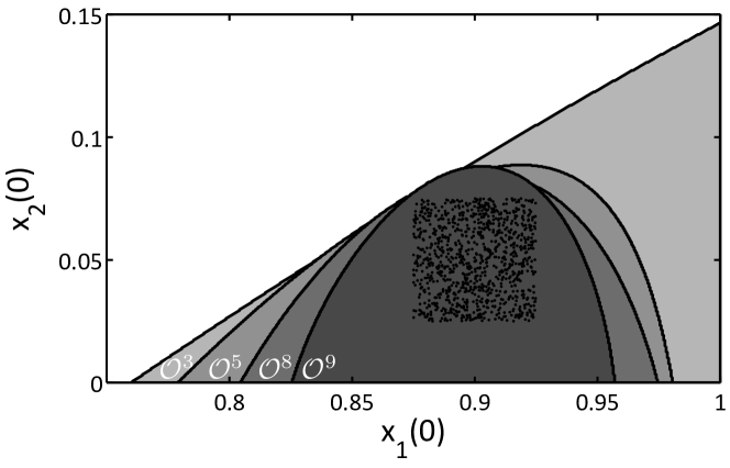
Figure 1: Set-based estimation of consistent parameters and initial conditions. Consistent samples (black dots) were determined by uniform sampling from $\mathcal{X}$ and subsequent numerical integration. Converging hierarchy of outer-approximations $\mathcal{O}^{d}$ with $d=3,5,8,9$ for estimation of $x_{1}(0)$, $x_{2}(0)$.

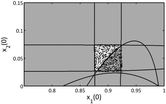
Figure 2: Set-based estimation of consistent parameters and initial conditions. Consistent samples (black dots) were determined by uniform sampling from $\mathcal{X}$ and subsequent numerical integration. Inner-approximations (white area) results from the union of outer-approximations (grey area and black lines) for $d=7$.

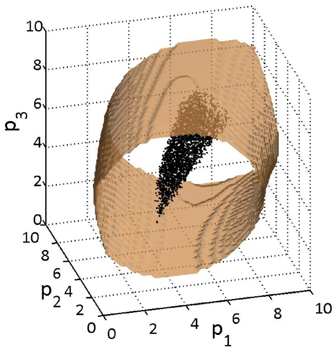
Figure 3: Set-based estimation of consistent parameters and initial conditions. Consistent samples (black dots) were determined by uniform sampling from $\mathcal{X}$ and subsequent numerical integration. Outer-approximations ($d=3$) of consistent initial conditions $x_{1}(0)$, $x_{2}(0)$ and parameters $p_{1},p_{2},p_{3}$ projected numerically onto the parameter space.

We consider a biochemical reaction network in which the substrate $x_{1}$ is enzymatically converted into a product via intermediary complex $x_{2}$ [25]. The continuous-time dynamics is given by:

$$\begin{array}[]{rcl}\dot{x}_{1}(t)&=&-p_{1}\,x_{1}(t)\bigl{(}1-x_{2}(t)\bigr{)}+p_{2}\,x_{2}(t),\\ \dot{x}_{2}(t)&=&\phantom{-}p_{1}\,x_{1}(t)\bigl{(}1-x_{2}(t)\bigr{)}-\bigl{(}p_{2}+p_{3}\bigr{)}\,x_{2}(t).\end{array}$$ (39)

The following constraints on the parameters and states were used:

$$\mathcal{X}:\left\{\begin{array}[]{rcll}(p_{i}-0.1)(10-p_{i})&\geq&0,&i=1,2,3,\\ x_{i}(1-x_{i})&\geq&0,&i=1,2.\end{array}\right.$$

Measurement constraints $\mathcal{X}_{k}$ were generated from a simulated nominal trajectory with $p_{1}=p_{2}=p_{3}=5.05,x_{1}(0)=0.9$ and $x_{2}(0)=0.05$. An absolute uncertainty of $\pm 0.025$ was added to the nominal values at the measurement time points $t_{0}=0,t_{1}=0.3,t_{2}=1$ to obtain $\mathcal{X}_{0}$, $\mathcal{X}_{1}$, $\mathcal{X}_{2}$. Thus, at each time-point four constraints were used, which results in $m_{c}=4\cdot 3$. To avoid numerical troubles, note that the dynamics (39) and $\mathcal{X}$ were scaled such that the values of the parameters range from 0 to 1.

As can be seen in Figure 1, the sequence of outer-approximations $\mathcal{O}^{d}$ converges to the consistent parameter set for increasing $d$. Using YALMIP and Sedumi, the solving time was about 5 seconds for $d=3$, and 40 minutes for $d=9$.

The inner-approximation in Figure 2 corresponds to the complement (in $\mathcal{X}$) of the union of twelve outer-approximations $\mathcal{O}(\mathcal{C}_{i})$. However, only eight outer-approximations are shown since the other four were empty. Solving time was on average 5 minutes per problem.

In addition we determined the outer-approximation of consistent initial conditions $x_{1}(0),x_{2}(0)$ and parameters $p_{1},p_{2},p_{3}$, see Figure 3. Solving time was about 4 hours.

Note that the inconsistency certificates derived in Section 4.3 could also be used to invalidate entire regions in the space of the parameters and initial conditions.

6 Discussion and Conclusions

Occupation measures are a classical tool in kinetic theory, statistical physics, optimal transport, Markov decision processes, amongst others. In a broad perspective, the potential of occupation measures and subsequent convex relaxations are not often used in systems control. We used occupation measures to approximate consistent parameter sets for continuous-time nonlinear systems without the need of numerical integration. A particular feature of the derived approximations is the (almost uniform) convergence to the true (possibly nonconvex) consistent parameter set. As demonstrated at the example, outer- and inner-approximations can be obtained even though only few measurements with relatively large error are used. Tighter approximations are expected if more measurements are used, or if e. g. outer-approximations are iteratively used to refine the results as it proved useful for linear relaxations [26, 21, 3].

While inconsistency certificates can be used to prove inconsistency of entire models or parameter regions, the outer- and inner-approximations can be used to get the shape of the consistent parameter set. Such a description of the outer-approximation by a single polynomial can be very useful in some applications. In other cases different types of representations like a collection of half-spaces might be more beneficial. The inconsistency certificates could also be used to derive in an iterative and recursive manner either outer bounding boxes or a description of the consistent set using a bisection algorithms (cf. [26]).

A drawback of the presented approach is the computational workload resulting from the LMI constraints. Theoretically, the resulting problems can be solved in polynomial time w.r.t. the input size. However, due to the size limitations of state-of-the-art SDP solvers, this approach is at the moment restricted to problems of small dimensions. An alternative could be the use of LP relaxations for larger dimensional systems. Note that the specific geometry of the LMI constraints makes these relaxations typically much more accurate than the LP relaxations and a trade-off between accuracy and problem size has to be made, see in particular the discussion in [12, Section 5.4.2].

As an interesting extension, one could consider statistical information, i. e. further constraints on the moments of the occupation measures. Here we assumed no more information such as statistics or probability distributions to be given. In many applications where there is a limited number of replicates, i. e. too few to obtain a meaningful statistic, this is actually the case. However, statistical information can be included if the data are polynomial or information about moments are available [12, 23].

References

- [1] J. Anderson, A. Papachristodoulou. On validation and invalidation of biological models. BMC Bioinformatics, 10:132, 2009.
- [2] M. Berz, K. Makino. Verified integration of ODEs and flows using differential algebraic methods on high-order taylor models. Reliable Comput. 4(4):361–369, 1998.
- [3] S. Borchers, P. Rumschinski, S. Bosio, R. Weismantel, R. Findeisen. A set-based framework for coherent model invalidation and parameter estimation of discrete time nonlinear systems. Proc. IEEE Conf. Decision and Control, Shanghai, China, 2009.
- [4] V. Cerone, D. Piga, D. Regruto. Set-membership error-in-variables identification through convex relaxation techniques. IEEE Trans. Automat. Control, 57(2):517–522, 2012.
- [5] B. D. Craven, J. J. Koliha. Generalizations of Farkas’ theorem. SIAM J. Math. Anal. 8(6):983–997, 1977.
- [6] D. Fey, E. Bullinger. Limiting the parameter search space for dynamic models with rational kinetics using semi-definite programming. Proc. IFAC Symposium on Computer Applications in Biotechnology, Leuven, Belgium, 2010.
- [7] D. Henrion, M. Korda. Convex computation of the region of attraction of polynomial control systems, arXiv:1208.1751, Aug. 2012.
- [8] L. Jaulin, M. Kieffer, O. Didrit, E. Walter. Applied interval analysis with examples in parameter and state estimation, robust control and robotics. Springer-Verlag, Berlin, 2001.
- [9] T. Johnson, W. Tucker. Rigorous parameter reconstruction for differential equations with noisy data. Automatica, 44:2422–2426, 2008.
- [10] M. Korda, D. Henrion, C. N. Jones. Inner approximations of the region of attraction for polynomial dynamical systems, arXiv:1210.3184, Oct. 2012.
- [11] L. Küpfer, U. Sauer, P. A. Parrilo. Efficient classification of complete parameter regions based on semidefinite programming. BMC Bioinformatics, 8(1):12, 2007.
- [12] J. B. Lasserre. Moments, positive polynomials and their applications. Imperial College Press, London, UK, 2009.
- [13] Y. Lin, M. Stadtherr. Validated solutions of initial value problems for parametric ODEs. Appl. Numer. Math. 57(10):1145–1162, 2007.
- [14] I. Mezić, T. Runolfsson. Uncertainty propagation in dynamical systems. Automatica, 44:3003–3013, 2008.
- [15] M. Milanese. Estimation theory for nonlinear models and set membership uncertainty. Automatica, 27:403–408, 1991.
- [16] N. Nedialkov, K. Jackson, G. Corliss. Validated solutions of initial value problems for ordinary differential equations. Appl. Math. Comput. 105:21–68, 1999.
- [17] S. Prajna. Barrier certificates for nonlinear model validation. Automatica, 42(1):117–126, 2006.
- [18] S. Prajna, A. Rantzer. Convex programs for temporal verification of nonlinear dynamical systems. SIAM J. Control Optim. 46(3):999–1021, 2007.
- [19] T. Raïssi, N. Ramdani, Y. Candau. Set membership state and parameter estimation for systems described by nonlinear differential equations. Automatica, 40(10):1771–1777, 2004.
- [20] A. Rauh, M. Brill, C. Günther. A novel interval arithmetic approach for solving differential-algebraic equations with ValEncIA-IVP. Int. J. Appl. Math. Comput. Sci. 19:381–397, 2009.
- [21] P. Rumschinski, S. Borchers, S. Bosio, R. Weismantel, R. Findeisen. Set-base dynamical parameter estimation and model invalidation for biochemical reaction networks. BMC Syst. Biol., 4:69, 2010.
- [22] P. Rumschinski, D. S. Laila, S. Borchers, R. Findeisen. Influence of discretization errors on set-based parameter estimation. Proc. IEEE Conf. Decision and Control, Atlanta, Georgia, 2010.
- [23] C. Savorgnan, J. B. Lasserre, M. Diehl. Discrete-time stochastic optimal control via occupation measures and moment relaxations. Proc. joint IEEE Conf. Decision and Control and Chinese Control Conf. 2009.
- [24] J. K. Scott, P. I. Barton. Improved relaxations for the parametric solutions of ODEs using differential inequalities. J. Global Optim., in press, 2013.
- [25] S. Schnell, M. J. Chappell, N. D. Evans, M. R. Roussel. The mechanism distinguishability problem in biochemical kinetics: the single-enzyme, single-substrate reaction as a case study. Comptes rendus biologies, 329(1):51–61, 2006.
- [26] S. Streif, A. Savchenko, P. Rumschinski, S. Borchers, R. Findeisen. ADMIT: a toolbox for guaranteed model invalidation, estimation and qualitative-quantitative modeling. Bioinformatics, 28(9):1290–1291, 2012.