A parameter estimation method based on random slow manifolds

Abstract

A parameter estimation method is devised for a slow-fast stochastic dynamical system, where often only the slow component is observable. By using the observations only on the slow component, the system parameters are estimated by working on the slow system on the random slow manifold. This offers a benefit of dimension reduction in quantifying parameters in stochastic dynamical systems. An example is presented to illustrate this method, and verify that the parameter estimator based on the lower dimensional, reduced slow system is a good approximation of the parameter estimator for original slow-fast stochastic dynamical system.

Mathematics Subject Classifications (2010)

Primary 60H30; Secondary 60H10; 37D10.

Keywords

Parameter estimation; Slow-fast system; Random slow manifold; Quantifying uncertainty; Numerical optimization

1 Introduction

Invariant manifolds provide geometric structures for understanding dynamical behavior of nonlinear systems under uncertainty. Some systems evolve on fast and slow time scales, and may be modeled by coupled singularly perturbed stochastic ordinary differential equations (SDEs). A slow-fast stochastic system may have a special invariant manifold called a random slow manifold that capture the slow dynamics.

We consider a stochastic slow-fast system

$$\dot{x}=A{x}+f(x,y),\quad x(0)=x_{0}\in\mathbb{R}^{n},$$ (1)

$$\dot{y}=\frac{1}{\varepsilon}B{y}+\frac{1}{\varepsilon}g(x,y)+\frac{\sigma}{\sqrt{\varepsilon}}\dot{W}_{t},\quad y(0)=y_{0}\in\mathbb{R}^{m},$$ (2)

where $A$ and $B$ are matrices, $\varepsilon$ is a small positive parameter measuring slow and fast scale separation, $f$ and $g$ are nonlinear Lipschitz continuous functions with Lipschitz constant $L_{f}$ and $L_{g}$ respectively, $\sigma$ is a noise intensity constant, and $\{W_{t}:t\in\mathbb{R}\}$ is a two-sided $\mathbb{R}^{m}$-valued Wiener process (i.e., Brownian motion) on a probability space $(\Omega,\mathcal{F},{\mathbb{P}})$. Under a gap condition and for $\varepsilon$ sufficiently small, there exists a random slow manifold $y=h^{\varepsilon}(\xi,\omega)$, $\omega\in\Omega$, as in [13, 5], for slow-fast stochastic system (1)-(2). When the nonlinearities $f,g$ are only locally Lipschitz continuous but the system has a random absorbing set (e.g., in mean-square norm), we conduct a cut-off of the original system. The new system will have a random slow manifold which captures the original system's slow dynamics.

The random slow manifold is the graph of a random nonlinear mapping $h^{\varepsilon}(\xi,\omega)=\sigma\eta^{\varepsilon}(\omega)+~{}\tilde{h}^{\varepsilon}(\xi,\omega)$, with $\tilde{h}^{\varepsilon}(\xi,\omega)$ determined by a Lyapunov-Perron integral equation [5],

$$\tilde{h}^{\varepsilon}(\xi,\omega)=\frac{1}{\varepsilon}\int_{-\infty}^{0}e^{-\frac{B}{\varepsilon}s}g(x(s,\omega,\xi),y(s,\omega,\xi)+\sigma\eta^{\varepsilon}(\theta_{s}\omega))\,ds,$$

with $\eta^{\varepsilon}(\theta_{t}\omega)=\frac{1}{\sqrt{\varepsilon}}\int_{-\infty}^{t}e^{\frac{B}{\varepsilon}(t-s)}\,dW_{s}$ and $\eta^{\varepsilon}(\omega)=\frac{1}{\sqrt{\varepsilon}}\int_{-\infty}^{0}e^{-\frac{B}{\varepsilon}s}\,dW_{s}$. The random slow manifold exponentially attracts other solution orbits. We will find an analytically approximated random slow manifold for sufficiently small $\varepsilon$, in terms of an asymptotic expansion in $\varepsilon$, as in [14, 15]. This slow manifold may also be numerically computed as in [7]. By restricting to the slow manifold, we obtain a lower dimensional reduced system of the original slow-fast system (1)-(2), for $\varepsilon$ sufficiently small

$$\dot{x}=A{x}+f(x,\tilde{h}^{\varepsilon}(x,\theta_{t}\omega)+\sigma\eta(\psi_{\varepsilon}\omega)),\quad x\in\;\;\mathbb{R}^{n},$$ (3)

where $\theta_{t}$ and $\psi_{\varepsilon}$ are defined in the next section.

If the original slow-fast system (1)-(2) contains unknown system parameters, but only the slow component $x$ is observable, we conduct parameter estimation using the slow system (3). Since the slow system is lower dimensional than the original system, this method offers an advantage in computational cost, in addition to the benefit of using only observations on slow variables.

This paper is arranged as follows. In the next section, we obtain an approximated random slow manifold and thus the random slow system. Then in Section 3, we present a method for parameter estimation on the slow manifold. Finally, a simple example is presented in Section 4 to illustrate our method.

2 Random slow manifold and its approximation

By a random transformation

$$\begin{matrix}\begin{pmatrix}X\\ Y\\ \end{pmatrix}:=\mathcal{V}_{\varepsilon}(\omega,x,y)=\begin{pmatrix}x\\ y-\sigma\eta^{\varepsilon}(\omega)\\ \end{pmatrix}\end{matrix},$$ (4)

we convert the SDE system (1)-(2) to the following system with random coefficients

$$\dot{X}(t)=AX(t)+f(X(t),Y(t)+\sigma\eta^{\varepsilon}(\theta_{t}\omega)),$$ (5)

$$\dot{Y}(t)=\frac{1}{\varepsilon}BY(t)+\frac{1}{\varepsilon}g(X(t),Y(t)+\sigma\eta^{\varepsilon}(\theta_{t}\omega)),$$ (6)

where $\eta^{\varepsilon}(\omega)=\frac{1}{\sqrt{\varepsilon}}\int_{-\infty}^{0}e^{-\frac{Bs}{\varepsilon}}\,dW_{s}$ is the stationary solution of linear system $dy^{\varepsilon}=\frac{B}{\varepsilon}y^{\varepsilon}dt+\frac{\sigma}{\sqrt{\varepsilon}}dW_{t}$. Here $\theta_{t}:\Omega\to\Omega$ is the Wiener shift implicitly defined by $W_{s}(\theta_{t}\omega)=W_{t+s}(\omega)-W_{t}(\omega)$. Note that $\eta^{\varepsilon}(\theta_{t}\omega)=\frac{1}{\sqrt{\varepsilon}}\int_{-\infty}^{t}e^{\frac{B}{\varepsilon}(t-s)}\,dW_{s}$.

Define a mapping (between random samples) $\psi_{\varepsilon}:\Omega\rightarrow\Omega$ implicitly by $~{}W_{t}(\psi_{\varepsilon}\omega)=\frac{1}{\sqrt{\varepsilon}}W_{t\varepsilon}(\omega)$. Then $\frac{1}{\sqrt{\varepsilon}}W_{t\varepsilon}(\omega)$ is also a Wiener process with the same distribution as $W_{t}(\omega)$. Moreover, $\eta^{\varepsilon}(\theta_{t\varepsilon}\omega)$ and $\eta^{\varepsilon}(\omega)$ are identically distributed with $\eta(\theta_{t}\psi_{\varepsilon}\omega)=\int_{-\infty}^{t}e^{B(t-s)}\,dW_{s}(\psi_{\varepsilon}\omega)$ and $\eta(\psi_{\varepsilon}\omega)=\int_{-\infty}^{0}e^{-Bs}\,dW_{s}(\psi_{\varepsilon}\omega)$, respectively.

By a time change $\tau=t/\varepsilon$ and using the fact that $\eta^{\varepsilon}(\theta_{\tau\varepsilon}\omega)$ and $\eta(\theta_{\tau}\psi_{\varepsilon}\omega)$ are identically distributed, the system (5)-(6) is reformulated as

$$X^{\prime}=\varepsilon[AX+f(X,Y+\sigma\eta(\theta_{\tau}\psi_{\varepsilon}\omega))],$$ (7)

$$Y^{\prime}=BY+g(X,Y+\sigma\eta(\theta_{\tau}\psi_{\varepsilon}\omega)),$$ (8)

where ${}^{\prime}=\frac{d}{d\tau}$.

We make the following two hypotheses.

$\mathbf{H1}$: There are positive constants $\alpha$, $\beta$ and $K$, such that for every $x\in\mathbb{R}^{n}$ and $y\in\mathbb{R}^{m}$, the following exponential estimates hold:

$$|e^{At}x|_{\mathbb{R}^{n}}\leq Ke^{\alpha t}|x|_{\mathbb{R}^{n}},\quad t\leq 0;\quad\quad|e^{Bt}y|_{\mathbb{R}^{m}}\leq Ke^{-\beta t}|y|_{\mathbb{R}^{m}},\quad t\geq 0.$$

$\mathbf{H2}$: $\beta>KL_{g}$.

Then there exists a random slow manifold $\mathcal{\tilde{M}}^{\varepsilon}(\omega)=\{(\xi,\tilde{h}^{\varepsilon}(\xi,\omega)):\xi\in\mathbb{R}^{n}\}$ for the random system (5)-(6), with $\tilde{h}^{\varepsilon}$ being expressed as follows [5, 12],

$$\tilde{h}^{\varepsilon}(\xi,\omega)=\frac{1}{\varepsilon}\int_{-\infty}^{0}e^{-\frac{B}{\varepsilon}s}g(X(s,\omega,\xi),Y(s,\omega,\xi)+\sigma\eta^{\varepsilon}(\theta_{s}\omega))\,ds.$$

We can get a small $\varepsilon$ approximation for $\tilde{h}^{\varepsilon}$. Start with the expansion $Y=Y_{0}+\varepsilon Y_{1}+\mathcal{O}(\varepsilon^{2})$ and the integral expression $X=X(0)+\varepsilon\int_{0}^{\tau}[AX+f(X,Y+\sigma\eta(\theta_{r}\psi_{\varepsilon}\omega))]\,dr$ in the system (7)-(8). Using the Taylor expansions of $f(X,Y+\sigma\eta(\theta_{\tau}\psi_{\varepsilon}\omega))$ and $g(X,Y+\sigma\eta(\theta_{\tau}\psi_{\varepsilon}\omega))$ at point $(x_{0},Y_{0}+\sigma\eta(\theta_{\tau}\psi_{\varepsilon}\omega))$ and denoting $\xi=~{}X(0)$, we obtain

$$\tilde{h}^{\varepsilon}(\xi,\omega)=~{}\tilde{h}_{d}^{\varepsilon}(\xi,\omega)+~{}\varepsilon\tilde{h}_{1}^{\varepsilon}(\xi,\omega)+~{}\mathcal{O}(\varepsilon^{2}),$$ (9)

for $\varepsilon$ sufficiently small, with

$$\tilde{h}_{d}^{\varepsilon}(\xi,\omega)=\int_{-\infty}^{0}e^{-Bs}g(\xi,Y_{0}(s)+\sigma\eta(\theta_{s}\psi_{\varepsilon}\omega))\,ds,$$ (10)

and

$$\tilde{h}_{1}^{\varepsilon}(\xi,\omega) = \int_{-\infty}^{0}e^{-Bs}\Big{\{}g_{x}(\xi,Y_{0}(s)+\sigma\eta(\theta_{s}\psi_{\varepsilon}\omega))\big{[}As\xi+\int_{0}^{s}f(\xi,Y_{0}(r)+\sigma\eta(\theta_{r}\psi_{\varepsilon}\omega))\,dr\big{]}$$ (11)

$$\quad\quad\quad\quad\quad\quad+g_{y}(\xi,Y_{0}(s)+\sigma\eta(\theta_{s}\psi_{\varepsilon}\omega))Y_{1}(s)\Big{\}}\,ds,$$

where $Y_{0}(t)$ and $Y_{1}(t)$ satisfy the following random differential equations, respectively

$$\begin{cases}Y^{\prime}_{0}(\tau)=BY_{0}(\tau)+g(\xi,Y_{0}(\tau)+\sigma\eta(\theta_{\tau}\psi_{\varepsilon}\omega)),\\ Y_{0}(0)=h_{d}^{\varepsilon}(0,\omega),\end{cases}$$ (12)

and

$$\begin{cases}Y^{\prime}_{1}(\tau)=\big{[}B+g_{y}(\xi,Y_{0}(\tau)+\sigma\eta(\theta_{\tau}\psi_{\varepsilon}\omega))\big{]}Y_{1}(\tau)\\ \quad\quad\quad\quad+g_{x}(\xi,Y_{0}(\tau)+\sigma\eta(\theta_{\tau}\psi_{\varepsilon}\omega))\big{\{}A\tau\xi+\int_{0}^{\tau}f(\xi,Y_{0}(s)+\sigma\eta(\theta_{s}\psi_{\varepsilon}\omega))\,ds\big{\}},\\ Y_{1}(0)=h_{1}^{\varepsilon}(0,\omega).\end{cases}$$ (13)

Noticing that $\eta^{\varepsilon}(\omega)$ and $\eta(\psi_{\varepsilon}\omega)$ have identical distribution, together with the fact that

$$\eta^{\varepsilon}(\omega)=\frac{1}{\sqrt{\varepsilon}}\int_{-\infty}^{0}e^{-\frac{Bs}{\varepsilon}}\,dW_{s}=\frac{1}{\sqrt{\varepsilon}}\int_{-\infty}^{t}e^{\frac{B(t-u)}{\varepsilon}}\,dW_{u}=\eta^{\varepsilon}(\theta_{t}\omega),\quad u=s+t,$$

we see that $\eta^{\varepsilon}(\theta_{t}\omega)$ and $\eta(\psi_{\varepsilon}\omega)$ are identically distributed. Recall the transformation introduced in the beginning of this section $X(t)=x(t)$ and $Y(t)=y(t)-\sigma\eta^{\varepsilon}(\theta_{t}\omega)$. We thus obtain a lower dimensional, slow stochastic system on the slow manifold,

$$\dot{x} = Ax+f(x,\tilde{h}^{\varepsilon}(x,\theta_{t}\omega)+\sigma\eta(\psi_{\varepsilon}\omega)),$$ (14)

Moreover, $\hat{h}^{\varepsilon}(\xi,\omega)=\tilde{h}_{d}^{\varepsilon}(\xi,\omega)+\varepsilon\tilde{h}_{1}^{\varepsilon}(\xi,\omega)$ is an approximation or a first order truncation of $\tilde{h}^{\varepsilon}(\xi,\omega)$, and hence we have an approximate slow system

$$\dot{x} = Ax+f(x,\hat{h}^{\varepsilon}(x,\theta_{t}\omega)+\sigma\eta(\psi_{\varepsilon}\omega)).$$ (15)

This is the slow system we will work on for parameter estimation in the next section.

3 Parameter estimation on a random slow manifold

If the original slow-fast system (1)-(2) contains an unknown system parameter $a$, but only the slow component $x$ is observable, we can conduct parameter estimation using the slow system (15). In fact, this unknown parameter $a$ is carried over to the slow system (15) which is now rewritten as

$$\dot{x} = Ax+f(x,\hat{h}^{\varepsilon}(x,\theta_{t}\omega)+\sigma\eta(\psi_{\varepsilon}\omega),a),\;\;x\in\mathbb{R}^{n},$$ (16)

for $\varepsilon$ sufficiently small.

Since this slow system is lower dimensional than the original system, this method offers an advantage in computational cost, in addition to a benefit of using only observations on slow variables. It is often more feasible to observe slow variables than fast variables [3].

Assume that we have observation, $x_{ob}$, on the slow component $x$ only, and let us estimate the system parameter $a$. An estimator $a_{E}^{S}(\varepsilon)$ for $a$ may be obtained with existing techniques as reviewed in our earlier work [16] or [3, 6] and references therein. Here the subscript $S$ indicates that the parameter estimation is conducted on the slow system (16). For example, $a_{E}^{S}(\varepsilon)$ may be obtained by minimizing the objective function $F(a)\triangleq{\mathbb{E}}||x_{ob}-x||^{2}_{\mathbb{R}^{n}}$.

We then compare this estimator $a_{E}^{S}(\varepsilon)$ with the estimator, $a_{E}(\varepsilon)$ (without superscript $S$), based on the original slow-fast system (1)-(2), when observations $x_{ob},y_{ob}$ are available for both components $x,y$. For example, $a_{E}(\varepsilon)$ may be obtained by minimizing the objective function $\mathbb{F}(a)\triangleq{\mathbb{E}}[||x_{ob}-x||^{2}_{\mathbb{R}^{n}}+||y_{ob}-y||^{2}_{\mathbb{R}^{n}}]$.

A stochastic Nelder-Mead method is used to minimize the objective functions. In the next section, we demonstrate this method with an example.

4 An example

In this section, we demonstrate our parameter estimation method based on random slow manifolds by a simple example.

Example 1.

Consider a slow-fast stochastic system

$$\dot{x} = 0.001x-axy,\quad x(0)=x_{0}\in\mathbb{R},$$ (17)

$$\dot{y} = \frac{1}{\varepsilon}(-y+\frac{1}{600}x^{2})+\frac{\sigma}{\sqrt{\varepsilon}}\dot{W}_{t},\quad y(0)=y_{0}\in\mathbb{R},$$ (18)

where $a$ is a real unknown positive parameter, $\varepsilon$ is a small positive scale separation constant, $\sigma$ is a constant noise intensity, and $W_{t}$ is a scalar Wiener process.

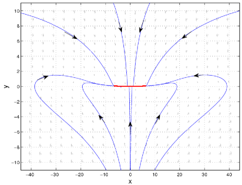
See Figure 1 for a phase portrait of the corresponding deterministic system ($\sigma=0$).

Figure 1: Deterministic dynamics – Phase portrait for $\dot{x}=0.001x-xy$, $\dot{y}=\frac{1}{\varepsilon}(-y+\frac{1}{600}x^{2})$ with $\varepsilon=\frac{1}{6}$: The global attractor is clearly seen (Red or thick curve within $-7<x<7$ and near the $x-$axis).

In this system, the nonlinear terms are not global Lipschitz. But if additionally it has an absorbing set, we can cut-off the nonlinearities without affecting the long time, slow dynamics (almost surely). Indeed, for arbitrary constants $M$ and $K$, we have

$$dx^{2} = 2x\,dx=(0.002x^{2}-2ax^{2}y)\,dt,$$

$$d(My-K)^{2} = 2(My-K)M\,dy+M^{2}\,d[y,y]$$

$$= \big{(}-\frac{2M^{2}}{\varepsilon}y^{2}+\frac{M^{2}}{300\varepsilon}x^{2}y+\frac{2MK}{\varepsilon}y-\frac{MK}{300\varepsilon}x^{2}+\frac{M^{2}\sigma^{2}}{\varepsilon}\big{)}dt+2M(My-K)\frac{\sigma}{\sqrt{\varepsilon}}\,dW_{t}.$$

Therefore,

$$d\big{(}\frac{M^{2}}{300\varepsilon}x^{2}+2a(My-K)^{2}\big{)}$$ (19)

$$= -\frac{1}{\varepsilon}\big{(}\frac{M^{2}}{300\varepsilon}x^{2}+2a(My-K)^{2}\big{)}\,dt-\frac{2aM^{2}}{\varepsilon}y^{2}\,dt+\frac{0.002M^{2}-2aMK+M^{2}/\varepsilon}{300\varepsilon}x^{2}\,dt$$

$$+\frac{2aK^{2}+2aM^{2}\sigma^{2}}{\varepsilon}\,dt+4aM(My-K)\frac{\sigma}{\sqrt{\varepsilon}}\,dW_{t}.$$

Taking $M=\varepsilon$, $K=\frac{1}{a\varepsilon}$, then we see that

$$\frac{0.002M^{2}-2aMK+M^{2}/\varepsilon}{300\varepsilon}=\frac{0.002\varepsilon^{2}-2+\varepsilon}{300\varepsilon}<0,\text{ for small }\varepsilon,$$

and

$$\frac{2aK^{2}+2aM^{2}\sigma^{2}}{\varepsilon}=\frac{2}{a\varepsilon^{3}}+2a\varepsilon\sigma^{2}.$$

Thus

$$\frac{d}{dt}\mathbb{E}\big{(}\frac{M^{2}}{300\varepsilon}x^{2}+2aM^{2}(y-K/M)^{2}\big{)}\leq-\frac{1}{\varepsilon}\mathbb{E}\big{(}\frac{M^{2}}{300\varepsilon}x^{2}+2aM^{2}(y-K/M)^{2}\big{)}+\frac{2}{a\varepsilon^{3}}+2a\varepsilon\sigma^{2}.$$ (20)

By the Gronwall inequality, we conclude that

$$\mathbb{E}\big{(}\frac{\varepsilon}{300}x^{2}+2a\varepsilon^{2}(y-\frac{1}{a\varepsilon^{2}})^{2}\big{)}$$ (21)

$$\leq \mathbb{E}\big{(}\frac{\varepsilon}{300}x_{0}^{2}+2a\varepsilon^{2}(y_{0}-\frac{1}{a\varepsilon^{2}})^{2}\big{)}e^{-\frac{t}{\varepsilon}}+(\frac{2}{a\varepsilon^{3}}+2a\varepsilon\sigma^{2})\varepsilon(1-e^{-\frac{t}{\varepsilon}})$$

$$\leq \big{(}\frac{\varepsilon}{300}x_{0}^{2}+2a\varepsilon^{2}(y_{0}-\frac{1}{a\varepsilon^{2}})^{2}\big{)}e^{-\frac{t}{\varepsilon}}+(\frac{2}{a\varepsilon^{2}}+2a\varepsilon^{2}\sigma^{2}).$$

This means, for fixed $\varepsilon$ and $a>0$, the dynamics of the system (17)-(18) will eventually stay in an ellipse (almost surely), i.e. there is a random absorbing set. We can then cut-off the nonlinearities outside this absorbing set to obtain a modified system which has, almost surely, the same long time, slow dynamics as the original system [7]. In the following calculations, we actually have omitted this cut-off procedure for simplicity.

By the random transformation (4), SDEs system (17)-(18) are converted into the following system

$$\dot{X} = 0.001X-aX(Y+\sigma\eta^{\varepsilon}(\theta_{t}\omega)),$$ (22)

$$\dot{Y} = -\frac{1}{\varepsilon}Y+\frac{1}{\varepsilon}\frac{1}{600}X^{2}.$$ (23)

Therefore, there exists an $\tilde{h}^{\varepsilon}$ satisfying

$$\tilde{h}^{\varepsilon}(\xi,\omega)=\frac{1}{\varepsilon}\int_{-\infty}^{0}e^{\frac{s}{\varepsilon}}\,\frac{X^{2}}{600}\,ds,$$ (24)

whose graph is a random slow manifold for the random system (22)-(23). In fact, $\tilde{h}^{\varepsilon}(\xi,\omega)$ has an approximation $\hat{h}^{\varepsilon}(\xi,\omega)$ (with error $\mathcal{O}(\varepsilon^{2})$),

$$\hat{h}^{\varepsilon}(\xi,\omega)=\frac{\xi^{2}}{600}+\varepsilon\big{(}-\frac{\xi^{2}}{300}0.001+\frac{\xi^{4}}{180000}a-\frac{\xi^{2}}{300}a\sigma\int_{-\infty}^{0}se^{s}\,dW_{s}\big{)}.$$ (25)

So the approximated slow system is

$$\dot{x} = 0.001x-ax\big{(}\sigma\eta(\psi_{\varepsilon}\omega)+\hat{h}^{\varepsilon}(x,\theta_{t}\omega)\big{)}.$$ (26)

with $\eta(\psi_{\varepsilon}\omega)=\int_{-\infty}^{0}e^{s}\,dW_{s}(\psi_{\varepsilon}\omega)$. We will illustrate that the parameter estimator for $a$ based on this low dimensional, reduced system (26) is a good approximation of the parameter estimator based on the original system (17)-(18).

Slow-fast system and random slow manifold

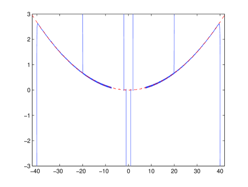
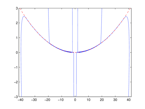
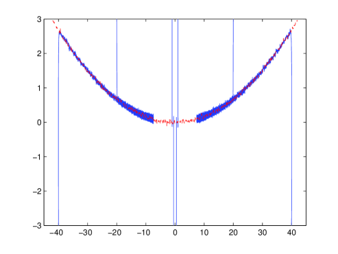
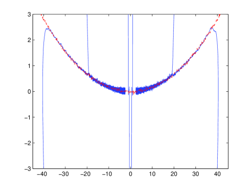
The random slow manifold is the graph of $h^{\varepsilon}(\xi,\omega)=\sigma\eta(\psi_{\varepsilon}\omega)+\tilde{h}^{\varepsilon}(\xi,\omega)$, where $\tilde{h}^{\varepsilon}$ is as in (24). It is a curve (depending on random samples). The random orbits of the system (17)-(18) approaches to this curve exponentially fast. Figures 2–3 show some orbits of the slow-fast system (17)-(18) and the approximate random slow manifold $\mathfrak{h}^{\varepsilon}(\xi,\omega)=\sigma\eta(\psi_{\varepsilon}\omega)+\hat{h}^{\varepsilon}(\xi,\omega)$, where $\hat{h}^{\varepsilon}$ is as in (25), with different $\sigma$ and $\varepsilon$ values.

The orbits of the system (17)-(18) decay quickly to the random slow manifold.

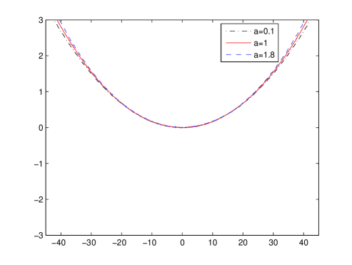
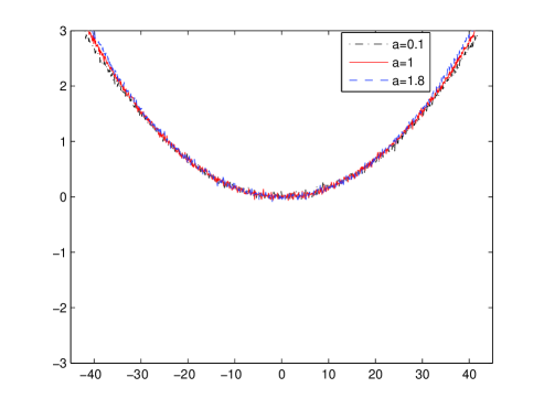
Figure 4 shows several samples or realizations of the random slow manifold with different $a$ values.

Figure 2: Orbits of slow-fast system (17)-(18) (blue curves) and its slow manifold expansion $\mathfrak{h}^{\varepsilon}(\xi,\omega)=\sigma\eta(\psi_{\varepsilon}\omega)+\hat{h}^{\varepsilon}(\xi,\omega)$ (red curve), where $\hat{h}^{\varepsilon}$ is as in (25), with $\sigma=0.01$ and $\varepsilon=0.01$: $a=0.1$ (left ) and $a=1$ (right).

Figure 3: Orbits of slow-fast system (17)-(18) (blue curves) and its slow manifold expansion $\mathfrak{h}^{\varepsilon}(\xi,\omega)=\sigma\eta(\psi_{\varepsilon}\omega)+\hat{h}^{\varepsilon}(\xi,\omega)$ (red curve), where $\hat{h}^{\varepsilon}$ is as in (25), with $\sigma=0.05$ and $\varepsilon=0.01$: $a=0.1$ (left ) and $a=1$ (right).

Figure 4: Random slow manifold expansion $\mathfrak{h}^{\varepsilon}(\xi,\omega)=\sigma\eta(\psi_{\varepsilon}\omega)+\hat{h}^{\varepsilon}(\xi,\omega)$, where $\hat{h}^{\varepsilon}$ is as in (25) with $\varepsilon=0.01$: $\sigma=0.01$ ( left ) and $\sigma=0.05$ (right).

Nelder-Mead method and stochastic Nelder-Mead method

The deterministic Nelder-Mead method (NM) is a geometric search method to find a minimizer of an objective function $F(a)$. Starting from an initial guess point, it generates a new point (reflection point, expand point, inside/outside contraction point or shrink point) by comparing function values, and thus get a better and better estimator until the smallest objective function value in this iteration reaches the termination value (prescribed error tolerance). The algorithm of the NM method and its improvements have been widely studied and utilized [1, 9, 10]. The method has its advantage that the objective function need not to be differentiable, and it can thus be used in various applications. As noted in [4, 11], the Nelder-Mead method is a widely used heuristic algorithm. Only very limited convergence results exist for a class of low dimensional (one or two dimensions) problems, such as in the case when the objective function $F$ is strictly convex [8]. For the numerical simulation, with analytical objective functions, Matlab function fminsearch can be used to find a minimizer.

However, when dealing with problems with noise, NM method has the disadvantage [2, 4] that it lacks an effective sample size scheme for controlling noise, as shrinking steps are sensitive to the noise in the objective function values and then may lead to the search in a wrong direction. In fact an analytical and empirical evidence is known for the false convergence [2] on stochastic function. So we use the stochastic Nelder-Mead simplex method (SNM) [4] to mitigate the possible mistakes in the stochastic setting. The newly developed Adaptive Random Search in [4] consists of a local search and a global search. It generates a new point and new objective function $\hat{F}=\sum\limits_{i=1}^{N(k)}F_{i}/N(k)$ in the $k-$th iteration with increasing number of the sample size scheme $N(k)$. A proper choice for $N(k)$ is $[\sqrt{k}]$, with $[c]$ the largest integer not bigger than $c$. Here $\sum\limits_{i=1}^{N(k)}F_{i}$ is the sum of $N(k)$ objective function values for $F$. SNM leads to the convergence of $F$ at search points to $\min\limits_{a}F(a)$ (and thus we obtain a minimizer $a^{*}$), with probability one.

Parameter estimation

To illustrate our method for parameter estimation on the random slow manifold, we fix $\varepsilon=0.01$ and $\sigma=0.01$ in the following numerical experiments.

We want to estimate the parameter $a$ by using both the original slow-fast system and the slow system, in order to demonstrate that the slow system is appropriate for parameter estimation, when $\varepsilon$ is sufficiently small.

Step 1: Generate observations

Take the true value $a=0.1$ (say) and numerically solve (17)-(18) with an initial condition $(x_{0},y_{0})$ to get $J$ samples of observational data $(x^{ij}_{ob},y^{ij}_{ob})$, $j=1,\cdots,J$ at time instants $t_{i}$, $i=1,\cdots,I$ (save these data).

Step 2: Estimator $a_{E}$ for the original slow-fast system

Take two initial guesses for the unknown system parameter $a=a_{0}$ and $a=a_{1}$ randomly and solve the original slow-fast system (17)-(18), with the same initial condition $(x_{0},y_{0})$ and time points $t_{i}$, $i=1,\cdots,I$. Thus we obtain $x^{i}$ and $y^{i}$ values which depend on $a$.

Using the stochastic Nelder-Mead Algorithm, we find a parameter estimator $a_{E}$ such that the objective function $F(a)\triangleq\mathbb{E}\sum\limits_{i=1}^{I}\sum\limits_{j=1}^{J}\big{(}(x^{i}-x^{ij}_{ob})^{2}+(y^{i}-y^{ij}_{ob})^{2}\big{)}$ is minimized.

Step 3: Estimator $a_{E}^{S}$ for the slow system

Take two initial guesses $a_{0}$ and $a_{1}$ randomly and solve the slow system (26) with the same initial condition $x_{0}$ at the same time instants $t_{i}$, $i=1,\cdots,I$. We thus obtain $X^{i}$ which depends on $a_{0}$ or $a_{1}$.

By the stochastic Nelder-Mead method as in Step 2, we find the parameter estimator $a_{E}^{S}$ by minimizing the objective function $\mathbb{F}(a)\triangleq~{}\mathbb{E}\sum\limits_{i=1}^{I}\sum\limits_{j=1}^{J}(X^{i}-~{}x^{ij}_{ob})^{2}$.

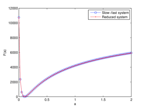
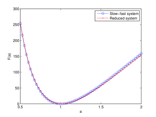
Figure 5: Objective function $F(a)$ for slow-fast system (17)-(18) and slow manifold reduced system (26), with $\sigma=0.01$ and $\varepsilon=0.01$: True values $a=0.1$ (left) and $a=1$ (right).

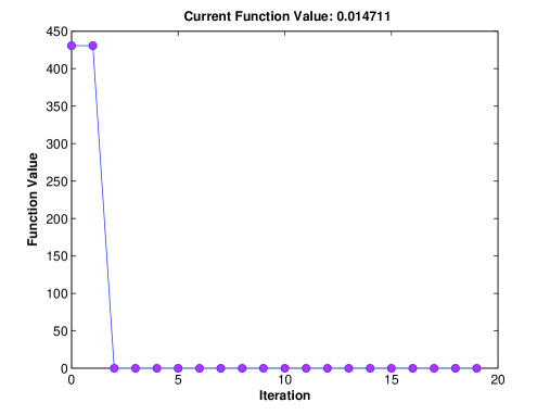
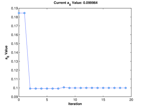
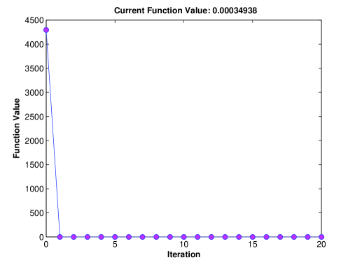
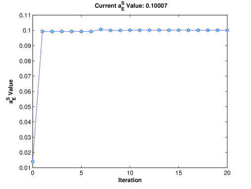
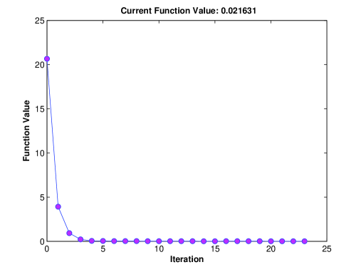
Figure 6: Objective function $F(a)$ and estimator $a_{E}$ (top) for slow-fast system (17)-(18); and objective function $\mathbb{F}(a)$ and estimator $a_{E}^{S}$ (bottom) for slow manifold reduced system (26): $\sigma=0.01$, $\varepsilon=0.01$ and true value $a=0.1$.

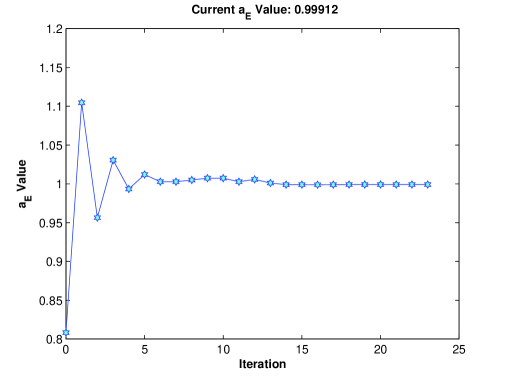
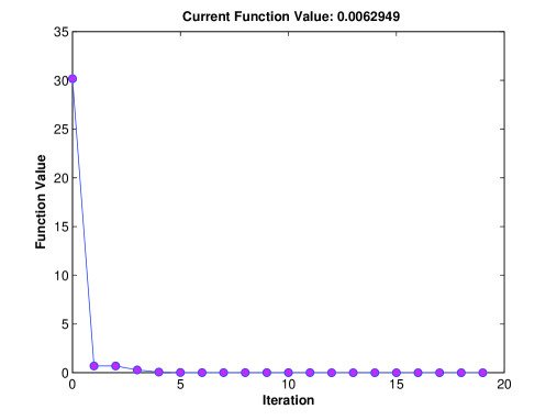
Figure 7: Objective function $F(a)$ and estimator $a_{E}$ (top) for slow-fast system (17)-(18), and objective function $\mathbb{F}(a)$ and estimator $a_{E}^{S}$ (bottom) for slow manifold reduced system (26): $\sigma=0.01$, $\varepsilon=0.01$ and true value $a=1$.

Numerical experiments

Figure 5 shows the objective functions $F(a)$ and $\mathbb{F}(a)$ with true $a=0.1$ (left) and $a=1$ (right). Here we used $30$ paths to get the expectation in the objective function.

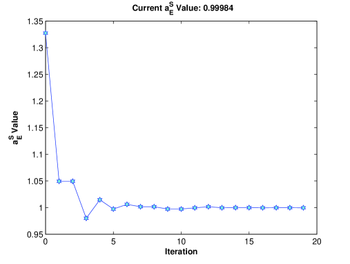
For $\varepsilon=0.01$ and $\sigma=0.01$, Figures 6 and 7 are objective function values and estimators of each iteration for slow-fast system (17)-(18) (top) and reduced system (26) (bottom) with $a=0.1$ and $a=1$, respectively.

We observe that, as proved in [4], the objective function value $F(a)$ tends to $\min\limits_{a}F(a)$(=0), while the minimizer or the parameter estimator $a_{E}$ provides an accurate estimation of the system parameter $a$. For sufficiently small $\varepsilon>0$, the objective function value $\mathbb{F}(a)$ for the slow system will also get closer and closer to $0$, and the minimizer or the parameter estimator $a_{E}^{S}$ is a good approximation of $a_{E}$.

References

• [1] R. Barati, Parameter Estimation of Nonlinear Muskingum Models Using Nelder-Mead Simplex Algorithm, J. Hydrol. Eng., 2011, 16, 946-954.
• [2] R. R. Barton and J. S. Ivey, Modifications of the Nelder-Mead Simplex Method for Stochastic Modification Response Optimization, Proceeding of the 1991 Winter Simulation Conference, 1991, 945-953.
• [3] J. P. N. Bishwal, Parameter Estimation in Stochastic Differential Equations, Springer, New York, 2007.
• [4] K. Chang, Stochastic Nelder-Mead simplex method - A new globally convergent direct search method for simulation optimization, European Journal of Operational Research, 220(2012), 684-694.
• [5] H. Fu, X. Liu and J. Duan, Slow manifolds for multi-time-scale stochastic evolutionary systems. Comm. Math. Sci., 2013, Vol. 11, No. 1, 141-162. arXiv:1205.0333 [math.PR]
• [6] I. A. Ibragimov and R. Z. Has'minskii, Statistical Estimation—Asymptotic Theory. Springer, New York, 1981.
• [7] X. Kan, J. Duan, I. G. Kevrekidis and A. J. Roberts, Simulating Stochastic Inertial Manifolds by a Backward-Forwand Approach. SIAM J. on Applied Dynamical Systems, in press, Vol. 12, 2013. arXiv:1206.4954 [math.DS].
• [8] J. C. Lagarias, J. A. Reeds, M. H. Wright and P. E. Wright, Convergence Properties of the Nelder-Mead Simplex Method in Low Dimensions, SIAM J. Optim., 1998, 9(1), pp 112-147.
• [9] J. Nocedal and S. J. Wright, Numerical Optimization, Springer Science+Business Media, LLC, New York, 2006.
• [10] N. Pham and B. M. Wilamowski, Improved Nelder Mead's Simplex Method and Applications, Journal of Computing, 2011, 3(3), 55-63.
• [11] C. J. Price, I. D. Coope and D. Byatt, A converging Variant of the Nelder-Mead Algorithm, Journal of Optimization Theorem and Applications, 113(1), 2002, pp. 5-19.
• [12] J. Ren, J. Duan and C. K. R. T. Jones, Approximation of Random Slow Manifolds and Settling of Inertial Particles under Uncertainty. Submitted to J. Dynamics & Diff. Eqns., 2012. arXiv:1212.4216
• [13] B. Schmalfuss and K. R. Schneider, Invariant manifolds for random dynamical systems with slow and fast variables. J. Dynamics & Diff. Eqns. 20 (2008), No. 1, 133–164.
• [14] X. Sun, J. Duan and X. Li, An impact of noise on invariant manifolds in nonlinear dynamical systems, J. Math. Phys. 51, 042702 (2010).
• [15] X. Sun, X. Kan and J. Duan, Approximation of invariant foliations for stochastic dynamical systems. Stochastics and Dynamics 12, No. 1, (2012), 1150011.
• [16] J. Yang and J. Duan, Quantifying Model Uncertainties in Complex Systems. Progress in Probability, 2011, Vol.65, 49-80.